| Issue |
A&A
Volume 668, December 2022
|
|
|---|---|---|
| Article Number | A50 | |
| Number of page(s) | 15 | |
| Section | Astronomical instrumentation | |
| DOI | https://doi.org/10.1051/0004-6361/202142820 | |
| Published online | 01 December 2022 | |
Iterative angular differential imaging (IADI): An exploration of recovering disk structures in scattered light with an iterative ADI approach
1
Anton Pannekoek Institute for Astronomy, University of Amsterdam,
PO Box 94249,
1090 GE
Amsterdam, The Netherlands
e-mail: This email address is being protected from spambots. You need JavaScript enabled to view it.
2
Leiden Observatory, Leiden University,
PO Box 9513,
2300 RA
Leiden, The Netherlands
Received:
1
December
2021
Accepted:
2
October
2022
Abstract
Context. Distinguishing the signal from young gas-rich circumstellar disks from the stellar signal in near-infrared (NIR) light is a difficult task. Multiple techniques have been developed over the years of which angular differential imaging (ADI) and polarimetric differential imaging (PDI) have been most successful. However, both techniques cope with drawbacks such as self-subtraction. To address these drawbacks, we explore iterative ADI (IADI) techniques to increase signal throughput in total intensity observations.
Aims. The aim of this work is to explore the effectiveness of IADI in recovering the self-subtracted regions of disks by applying ADI techniques iteratively.
Methods. IADI works by feeding back all positive signal of the result from standard ADI over multiple iterations. To determine the effectiveness of IADI, a model of a disk image is made and post-processed with IADI. We explored two versions of IADI, classical IADI, which uses the median of the data set to reconstruct the point spread function (PSF), and PCA-IADI, which uses principal component analysis to model the PSF. In addition, we explored masking based on polarimetric images and a signal threshold for feeding back signal.
Results. Asymmetries are a very important factor in recovering the disk because these lead to less overlap of the disk in the data set. In some cases, we were able to recover a factor ~75 more flux with IADI than with ADI. The Procrustes distance is used to quantify the impact of the algorithm on the scattering phase function. Depending on the level of noise and the ratio between the stellar signal and disk signal, the phase function can be recovered a factor 6.4 in Procrustes distance better than standard ADI. Amplification and smearing of noise over the image due to many iterations did occur. By using binary masks and a dynamic threshold this feedback was mitigated, but it is still a problem in the final pipeline. Finally, observations of protoplanetary disks made with VLT/SPHERE were processed with IADI giving rise to very promising results.
Conclusions. While IADI has problems with low-signal-to-noise-ratio (S/N) observations due to noise amplification and star reconstruction, higher S/N observations show promising results with respect to standard ADI.
Key words: techniques: image processing / methods: data analysis / protoplanetary disks / stars: pre-main sequence / infrared: planetary systems
© L. M. Stapper and C. Ginski 2022
 Open Access article, published by EDP Sciences, under the terms of the Creative Commons Attribution License (https://creativecommons.org/licenses/by/4.0), which permits unrestricted use, distribution, and reproduction in any medium, provided the original work is properly cited.
This article is published in open access under the Subscribe-to-Open model. This email address is being protected from spambots. You need JavaScript enabled to view it. to support open access publication.
1 Introduction
In recent years, scattered light observations with facilities such as the Spectro-Polarimetric High-contrast Exoplanet REsearch (SPHERE, Beuzit et al. 2019) imager and Gemini Planet Imager (GPI, Macintosh et al. 2014) have proven to be very successful in revealing the structures of circumstellar disks in which planetary systems are created. Structures such as rings (e.g., Ginski et al. 2016; van Boekel et al. 2017), spiral arms (e.g., Avenhaus et al. 2017; Follette et al. 2017; Monnier et al. 2019), asymmetric rings and gaps (e.g., Pohl et al. 2017; Benisty et al. 2018; Laws et al. 2020), and shadows (e.g., Stolker et al. 2016; Muro-Arena et al. 2020) have all been observed with scattered light imaging (see Benisty et al. 2022 for a recent overview of the field).
A key problem in optical and near-infrared (NIR) observations is that signal from the disk (or planet) is drowned out by the stellar speckle halo, which is several orders of magnitude brighter than disk-scattered light or planet thermal emission. Different high-contrast imaging techniques can be used to remove the stellar light. Polarimetric Differential Imaging (PDI) uses the (un)polarized nature of the (star) disk to disentangle light emitted by the star and light scattered by the disk (e.g., Kuhn et al. 2001; Apai et al. 2004). However, not all light scattered by the disk is polarized. The polarization can vary up to 15% depending on the scattering angle (Min et al. 2005), all the while depending on the dust grains and observation wavelength (Murakawa 2010). Therefore, a different technique is necessary to obtain the total scattered light intensity.
Angular differential imaging (ADI) is a high-contrast imaging technique used to remove stellar light from NIR or optical images, while retaining the light from off-axis faint planets or circumstellar material (Marois et al. 2006). This is done by making use of field rotation; while the stellar point spread function (PSF) keeps the same position with respect to the telescope, off-axis faint planets or circumstellar material will rotate. ADI is particularly useful for retrieving the total intensity of the scattered light or the thermal emission of young planets (which is typically only marginally polarized; see e.g., Stolker et al. 2017; van Holstein et al. 2021). Determining the total intensity is important for obtaining information about the dust grain properties (e.g., Tazaki et al. 2019) and planet emission (e.g., van Holstein et al. 2021) and for inferring scatter angles in combination with polarimetric observations (Ginski et al. 2021). While ADI works very well on point-like sources such as exoplanets (e.g., HR 8799 Marois et al. 2008, 2010; 51 Eri Macintosh et al. 2015; HIP 65426 Chauvin et al. 2017), it struggles with extended structures because of “self-subtraction” due to parts of the structure overlapping during the observation. This leads to a number of problems.
First, there is separation-dependent throughput. Due to the decrease in the length of the rotational arc with smaller separation from the central star, ADI throughput depends on angular separation. This leads to a suppression of disk signal in particular along the minor axis, which may turn ring-like radial substructures into “broken” arc-like structures. Importantly, this will also significantly alter the scattering phase function and suppress signal for the smallest scattering angles. Second, spatial filtering occurs. Self-subtraction depends on the spatial frequency of radial features. High-spatial-frequency features have a higher throughput than low-spatial-frequency features. This effectively results in a form of high-pass filtering. Such filtering is particularly problematic for young gas-rich disks, as these tend to have a more diffuse morphology than debris disks, which are often concentrated in sharper rings. Third, self-subtraction can lead to nontrivial deformation of spatial features, such as ring-like features in particular, which may be deformed such that they can be misinterpreted as spiral structures. Lastly, self-subtraction in ADI strongly biases the global disk-detection rate in scattered light toward exceptionally extended disks with high inclinations, while small or low-inclination disks may not be detected at all. For a general discussion of these effects, we refer to the overview given by Milli et al. (2012). For specific examples, in particular of separation-dependent throughput and spatial filtering, we refer to de Boer et al. (2016), Ginski et al. (2016) and Perrot et al. (2016).
Recent works explored different techniques used to improve ADI to limit self-subtraction and thus increase signal throughput (e.g., Pairet et al. 2018, 2021; Ren et al. 2018). Our work explores a technique called Iterative ADI (IADI), which is designed to solve the issue of self-subtraction present in ADI in order to obtain similar results to those obtained with PDI, but now using the full intensity of the scattered light. We are applying different data-processing strategies to improve throughput. Specifically, we combine the base concept of an iterative approach with classical ADI (cADI) and with principal component analysis(PCA)-based ADI. The latter approach is identical to the GreeDS (Greedy Disk Subtraction) algorithm presented in Pairet et al. (2021). We are expanding upon previous studies by including a data-masking strategy based on PDI observations and by performing a detailed performance analysis of all techniques.
In Sect. 2, the IADI reduction algorithm is explained and in Sect. 3.1 a simple scattered light model of a disk is made, which is put through IADI post-processing in subsequent sections. To quantify the recovery of the disk with IADI, two performance metrics are presented in Sect. 3.2, with particular emphasis on the recovery of the scattering phase function of the circumstellar disk (i.e., the scattering-angle-dependent brightness distribution of the disk). The effects of the elevation (i.e., distance above the horizon related to the amount of field rotation) and inclination of the science target and the speed at which IADI converges to a particular final result are explored in Sect. 3.3. The effects of the speckle field of the central star are analyzed in Sect. 3.4 and ways to suppress its affect on the reduction are presented in Sect. 3.5. Finally, IADI is applied to three SPHERE observations toward circumstellar disks in Sect. 4. Our results are summarized in Sect. 5.
2 Algorithm
ADI (and by extension, IADI) makes use of field rotation, which is the apparent rotation of an object in the field of view of an altitude-azimuth-mounted telescope due to the rotation of the Earth. Due to the point-source-like nature of the central star, the PSF of the star caused by the telescope (and observation conditions) will stay in the same orientation during the observation. On the other hand, any possible companion of the star, such as a planet or a protoplanetary disk, will rotate in the field of view of the telescope; see Cols. 0/1 in Fig. 1. Therefore, field rotation causes no change in the orientation of the signal that needs to be removed from the image (the star) and a change in the orientation of the signal that contains the science object (the disk). IADI expands upon ADI by performing this process iteratively on the same data set, and so part of the reduction process is the same as ADI (see the dashed box in Fig. 1).
First (Col. 0 of Fig. 1), a copy of the original data set is made. In the first iteration, Col. 1 contains the exact same data set as Col. 0. The stellar PSF is isolated by taking the median of the data set along the time axis (i.e., along the pixels at the same position in each image in the data set). Ideally, only the stellar PSF will remain; see Col. 2 of Fig. 1. In addition to taking the median, principal component analysis (PCA, Amara & Quanz 2012) is also explored in this work. With PCA, an image is decomposed into a set of functions, or principal components of the image, which, when combined linearly, can represent the original image. This approach is implemented based on the Python package PynPoint (Stolker et al. 2019). In practice, first the data are mean subtracted and then reconstructed via PCA with a specific number of principal components. The resulting PSF found via either the median approach (classical IADI, or cIADI) or via PCA (PCA-IADI) is subtracted from the original data set; see Col. 3 of Fig. 11.
After PSF subtraction, the images are rotated back, such that the science object in each image has the same orientation, see Col. 4 of Fig. 1. The images are then combined by taking the median; see Col. 5 of Fig. 1. Ideally, all signal coming from the science object is now recovered. However, this is rarely the case; hence the iterative nature of IADI. As shown in the bottom row of Fig. 2, with classical ADI, large parts of the disk are missing due to self-subtraction. Therefore, in the final step, all the positive signal is fed back by subtracting this from the original data set in Col. 0 and the process is repeated. In this way, Col. 1 contains less disk signal, and so less signal of the disk will be in the recovered PSF and consequently less of the disk is subtracted in the final step. After many iterations, more of the disk is recovered (see the bottom row of Fig. 2). We note that one can also feedback parts of the result instead of all positive signal with the use of a threshold or a mask; this is explored in Sect. 3.5. Asymmetry in the disk plays an important role in IADI (as it already does in standard ADI). The more asymmetric the disk, the faster the process will converge to a final image.
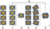 |
Fig. 1 Flowchart depicting the different steps in the IADI reduction process. 0. Copy of the original data set, which is used after every iteration. 1. The original data set minus the final result from step 5. If this is the first iteration, the data sets of step 0 and 1 are identical. Even after some iterations, some disk signal is left in this data set after subtracting the final result. This is shown as the gray dotted ellipses. 2. Take the median of the data set (cIADI) or construct the PSF with principal components after taking the mean of the data set (PCA-IADI). 3. Subtract the found PSF from each image in the original data set copied in step 0. 4. Derotate the data set such that the science object has the same orientation in all images. 5. Take the median of all derotated images to combine them and get the final result. 6. Feedback all positive signal of the final result from step 5 to step 1 and then repeat the process. |
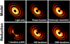 |
Fig. 2 Model used in this work together with a reduction with the IADI pipeline. The top panels show, from left to right, a ~1/r2 intensity dependence from the center of the disk, the addition of the phase function, and telescope resolution. The bottom panels present the recovered disk after 1, 100, and 1000 iterations. This shows that with classical ADI, large parts of the disk are not recovered due to self-subtraction, but that these can be recovered iteratively. All images use a log-scale to make the faint parts of the disk more visible. |
3 Model reduction
3.1 Model setup
To test IADI, we made a model of a disk in scattered light. This model is 400 × 400 pixels, each pixel having a physical size of 1 × 1 au. Multiple rings are implemented, inspired by observations of disks (e.g., HD 97048 Ginski et al. 2016; RX J1615 de Boer et al. 2016 and TW Hydrae van Boekel et al. 2017), see panel a in Fig. 2. A specific inclination and rotation is achieved using the warpAffine function from OpenCV (Bradski 2000). Young planet-forming disks are still gas rich and dust particles are stratified due to gas pressure along the vertical axis. Therefore, flaring is implemented in the model via an offset of the rings with respect to the center of the ring (see the detailed discussion in de Boer et al. 2016). For our disk model, we are using the power-law profile for the scattering surface height H and the separation r found by Ginski et al. (2016) for the disk around HD 97048. This profile describes the flaring discovered in this source reasonably well up to a separation of ~270 au. Considering that the model disk used will have a separation of 200 au, this formula will be sufficient to simulate the disk height2. Illumination effects of the central star are implemented via a ~1/r2 intensity dependence from the center of the disk, making the inner part of the disk brighter compared to the outer part. Moreover, the intensity also depends on the light scattering angle via the phase function. Because a physical model is beyond the scope of this work, a “pseudo” phase function is implemented to mimic the same asymmetries in light distribution seen in observed disks via I = cos ϕ, where the intensity I depends on the cosine of the azimuthal angle ϕ. This pseudo phase function depends on the azimuthal angle instead of a scattering angle on which a real phase function would depend. This makes the part of the disk facing toward the observer appear brighter than the part facing away in a fairly simple way. Lastly, the model is put through a Gaussian convolution kernel from the scipy ndimage package (Virtanen et al. 2020) to remove sharp edges and give a finite resolution to the model. The final three steps are shown in the top row of Fig. 2.
3.2 Performance metrics
To quantify how well the disk is recovered after IADI postprocessing, two main metrics are used. First, in Sect. 3.3 only the disk is processed by the IADI pipeline. Although this specklefree reduction is not representative of the reality of observation conditions with real stellar noise, this simplified case allows us to assess the impact of self-subtraction only on the disk. Second, in Sect. 3.4 the model is inserted into observations of a star, and thus cannot be directly compared to the model. Hence, the phase functions of the recovered disks will be compared to the phase function of the model via a Procrustes analysis.
Retrieved Flux Comparison
The first metric is the amount of retrieved flux compared to the inserted disk model. The original total flux of the disk is the sum of the values of each pixel in the original model. After every iteration, this recovered flux is compared to the original value of the model. The recovered flux (in %) is the ratio between the sum of the values of each pixel in the disk after some number of iterations divided by the sum of the values of each pixel in the original disk. In Fig. 3, one can see that the recovered flux increases rapidly in approximately the first 200 iterations, after which it increases linearly.
Contradictory to what one might expect, the total recovered flux increases to above 100%. This is due to numerical artifacts generated during the reduction process. The numerical noise is the noise introduced into the disk because of interpolation artifacts due to the many rotations during IADI processing. While in real observations this noise cannot be estimated, in this case the actual disk is known and therefore can be used to estimate the amount of noise introduced. The percentage of numerical noise depends on the interpolation kernel used; see Fig. 3. After careful consideration, nearest neighbor interpolation was found to introduce the least amount of noise into the image while still recovering the majority of the disk, given that enough images of the disk are present in the data set to still sample the disk well. Whether nearest-neighbor interpolation is the most optimal choice should be considered on a case-by-case basis. The numerical noise is calculated by subtracting the original disk from the recovered disk and summing all positive values. In this way, every pixel where the value is larger than the original disk remains, which should come from numerical artifacts. However, everywhere where the disk had self-subtraction, the numerical noise introduced is not measured, and so this only gives a lower limit on the numerical noise. Unfortunately, numerical artifacts will never be completely absent, but can be kept to a minimum by choosing the correct interpolation kernel (i.e., nearest-neighbor interpolation for any further reduction done in this work).
Lastly, the corrected flux is the recovered flux corrected for the numerical noise. After correcting the flux for the numerical noise, the total amount of flux indeed does not surpass 100%; see Fig. 3.
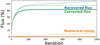 |
Fig. 3 Recovered flux, numerical noise, and corrected flux plotted against the number of iterations of a disk with an inclination of 45° and elevation of 85° processed with cIADI. Both spline interpolation (dashed lines) and nearest-neighbor interpolation (continuous lines) are shown. |
Procrustes Analysis
Ultimately, the recovery of the phase function is an important goal after post-processing the data. Hence, a “pseudo” phase function is recovered by summing all positive pixels in bins in the azimuthal direction, which is then smoothed by a Butterworth low pass filter. A Procrustes analysis is then used to analyze the recovered shapes of these phase functions (Dryden & Mardia 2016). The algorithm for comparing the recovered phase function and the model phase function works as follows. First, we translate the mean of the phase functions to the origin. Second, a uniform transformation is done via scaling the phase functions such that the root mean square of the distance to the origin is equal to one. Finally, to quantify the difference between the two phase functions, the Procrustes distance is computed via
![Mathematical equation: $ {d_{\Pr }} = {\left( {\sum\limits_{i = 1}^n {\left[ {{{\left( {{x_i} - {u_i}} \right)}^2} + {{\left( {{y_i} - {v_i}} \right)}^2}} \right]} } \right)^{1/2}}, $](/articles/aa/full_html/2022/12/aa42820-21/aa42820-21-eq1.png) (1)
(1)
in which (xi, yi) and (ui, vi) are the i-th coordinates of the recovered and model phase functions, respectively. The closer the Procrustes distance is to zero, the more similar the two phase functions are to each other. A Procrustes distance of zero means that, after removing translational and scaling factors, both functions have the exact same shape.
It should be noted that in Dryden & Mardia (2016), an extra step is mentioned in which any rotational differences are also removed. Considering that the phase functions are positioned in the same direction, this step was omitted. Furthermore, the models to which the recovered phase functions are compared to will be kept the same between all reductions. In this way all computed Procrustes distances can be compared to each other.
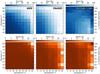 |
Fig. 4 Recovered flux and generated numerical noise with cIADI and PCA-IADI after 500 iterations for a grid of models with different inclinations and elevations. The corresponding amount of field rotation is indicated by the vertical axis on the right. The top row shows the recovered flux and the bottom row the numerical noise. The rightmost column shows the difference between PCA-IADI and cIADI. |
3.3 Tests on disk model only
To asses how well the self-subtracted areas of the disk can be recovered with IADI, we reduced a 9 × 9 grid of models for 500 iterations with cIADI and PCA-IADI for nine different inclinations and nine different elevations. The models are simulated at the Paranal observatory with the target at different declinations. For general applicability at other telescopes, the results are given in the elevation of the target and its corresponding amount of field rotation. In case of high latitudes, the results shown here are optimistic because of a much smaller amount of field rotation (see Appendix A). However, at these high latitudes, no major direct imaging facility exists. The model consists of 60 images (spaced over 1 h of observations) of 400 × 400 pixels each; see Fig. 2. These reductions can be seen in Fig. 4, in which the first and second rows show the amount of recovered flux and numerical noise after 500 iterations as percentages of the total flux of the original model for cIADI and PCA-IADI, respectively. The third column is the difference between the two techniques.
As presented in the recovered flux panels in Fig. 4, higher elevations and inclinations (more asymmetrical disks) are favorable for the recovery of the disk. The elevation of the disk determines both the total amount of field rotation and the speed at which the rotation occurs (see the vertical axis on the right of Fig. 4). The larger the elevation of the object, the more it will rotate during the observation if observed during its meridian passage. However, when the elevation is close to 90°, this rotation is almost instantaneous. Hence, even though the field rotation is maximal, the rotation in that case only happens in between two images. This gives rise to two sets of almost identical images, reducing the amount of flux recovered from the disk. In general, independently of the telescope latitude, the optimal amount of field rotation and rotation speed occur at an elevation of 85°, or a ~5° difference between the declination and latitude. The inclination (or similarly any asymmetry in the disk) affects the recovery of the disk as well. For higher inclinations (or more asymmetrical disks), when subtracting the median of the data set from the images, less self-subtraction will occur. For this reason, disks at greater inclinations are recovered better. Both the elevation and inclination combined give rise to the diagonal gradient going from the bottom left to the top right as seen in the panels of Fig. 4.
In general, more of the flux is recovered with PCA-IADI than with cIADI. The recovered flux is on average 25% higher for PCA-IADI than for cIADI. As shown by the panel of Fig. 4 with the differences in recovered flux between cIADI and PCA-IADI, PCA-IADI mainly improves upon the recovery of the disk with cIADI at high inclinations and low elevations or little field rotation. cIADI is more affected by the small differences between the images due to the low elevation, causing less flux to be recovered because more of the disk is self-subtracted. On the other hand, for PCA-IADI, the small evenly spaced rotations between every image are still enough for it to not remove the disk completely, resulting in better recovery of the disk than with cIADI. Going to higher elevations, the difference in recovered flux is less apparent. At these high elevations, more and faster field rotation occurs, giving rise to a data set essentially containing two similar sets of images, which is easier for PCA to fit to and more of the disk will be subtracted. Therefore, in practice, it would be best to apply PCA-IADI to data sets with images with relatively constant rotation between images, while cIADI can also be applied to data sets containing less evenly rotated images.
The noise generated while using the pipeline, especially when the stellar speckle halo is present, is an important factor in deciding which reduction technique to use. As the second column in Fig. 4 shows, the more the images need to be rotated, and the higher the asymmetry is in the disk, the more numerical noise is generated. While the latter is not as detrimental when using real observations, speckle noise will have the same effect, which is discussed in the following sections. The introduction of numerical noise at these higher elevations and inclinations originates from the interpolation while rotating the disk and sharp edges in the model due to the high inclination.
PCA-IADI generates more noise than cIADI (see Fig. 4); on average the amount of numerical noise is 3.3% higher with a maximum difference of 22.0%. This is especially problematic when iterating too many times over the data. Because PCA-IADI is also fitting to the numerical noise generated, this noise is amplified over time. Consequently, one needs to know the minimum number of iterations necessary to recover the disk. This is inferred from Fig. 5. This figure shows the number of iterations necessary to recover 99% of the amount of flux recovered after 500 iterations for cIADI (left) and PCA-IADI (right). In other words, it indicates how fast the models converge to a particular value. Figure 5 shows that, while an increased number of asymmetries in the disk (due to inclination) generates more numerical noise in the result, no more than 100 iterations are necessary to recover the disk. Consequently, the amount of numerical noise can be decreased by using less iterations for these highly asymmetric disks. For both cIADI and PCA-IADI, more than 500 iterations are necessary to recover the flux at intermediate elevations and low inclinations. PCA-IADI is especially slow in converging to a final result. This is likely due to the fact that PCA-IADI first subtracts the mean of the data set from each image before fitting the principal components, which are subtracted from the data set as well. This much more aggressively removes the common modes in the images of the data set than cIADI does, which results in a much slower convergence. For cIADI, the final amount of recovered flux in the bottom left part of the plot is already relatively low (see Fig. 4). The number of iterations to reach this low amount of flux is already reached after about 100 iterations, which explains the relatively fast converging speed in the bottom left of the plot for cIADI. While PCA-IADI does recover more, the high number of iterations necessary makes it more worthwhile to use cIADI for these low elevations (small amount of field rotation), so that the amount of noise introduced due to the iteration process is kept at a minimum.
In conclusion, the full disk can be recovered using both versions of IADI, depending on the elevation (or field rotation) and inclination (or asymmetry) of the disk. Due to the slow converging speed of PCA-IADI, cIADI is more suitable for increasingly symmetrical disks. PCA-IADI on the other hand favors highly asymmetrical disks. Due to differences in spacing between images depending on the elevation, cIADI should be used in datasets with large differences in rotation between images, while PCA-IADI works best for small rotational differences. Finally, PCA-IADI introduces the most noise to the reduction, and amplifies this. Hence, only a limited number of iterations should be done with it.
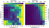 |
Fig. 5 Number of iterations necessary to reach 99% of the flux recovered after 500 iterations; i.e., the convergence speed. |
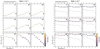 |
Fig. 6 Procrustes distance of cIADI normalized by the Procrustes distance obtained from cADI of the retrieved phase functions for different inclinations and elevations. The corresponding total field rotation is shown on the horizontal axis on top. The circles show the maximum value out of 500 iterations. The final values are shown as crosses. We note that the right panel has a different color scale from the left panel. |
3.4 Test on a model inserted into a star
The model was inserted into observations of the star GSC 08047-00232 made by SPHERE/IRDIS on the VLT. Both the SED of this system as well as the SPHERE polarimetric observations show that no disk resides around this star. In addition, the data were taken in the same observation mode as the majority of new disk observations (i.e., pupil-stabilized observations in polarimetric mode with the BB_H filter), and so the instrument characteristics should be similar to those used in most recent observations. This observation consisted of a total of 40 images instead of the previously used 60 images, but is still simulated with a 1 h observation time around meridian. The model and the star are combined by first normalizing the model and the data by dividing by their respective maximum values, then the normalized images are added together after multiplying them by a “ratio factor” of either 1 × 10⁻² or 1 × 10⁻³. For this section, four grids of reductions are made; see Figs. 6 and 7 for cIADI and PCA-IADI respectively. In addition, one specific case is shown: a model with an elevation of 85° and an inclination of 45° for both cIADI and PCA-IADI in Fig. 8.
The normalized Procrustes distance on the vertical axes in Figs. 6 and 7 can be interpreted as the factor by which the recovered phase function improved (or goodness-of-recovery) with respect to classical angular differential imaging (either via using the median or using PynPoint for cIADI and PCA-IADI, respectively). For both PCA-IADI and cIADI, the goodness-of-recovery clearly depends on the inclination and elevation of the object in the case of a ratio of 1 × 10⁻². In agreement with the previous section, for higher inclinations, the model reaches the highest possible improvement factor faster than for lesser inclined disks due to the increase in asymmetry. In general, cIADI can be run for a larger number of iterations than PCA-IADI in high-signal-to-noise-ratio (S/N) cases, while also improving the phase function recovery by up to a factor of 11.
When there are too many iterations, the recovered phase function goes above the intensity of the model phase function and may change shape, decreasing the goodness-of-recovery, as indicated by the crosses; especially for the high elevation and inclination cases. This can also be seen in the reduction for a 45° inclination and 85° elevation model for both a ratio of 1 × 10⁻² and 1 × 10⁻³ shown in Fig. 8. For high S/N, the original phase function shape is well recovered after only 10 iterations (left panel Fig. 8), with 100 iterations recovering the best fitting phase function compared to the original model. Larger numbers of iterations begin to reconstruct the star, which can be seen as signal in the center of the image (see Fig. 8). In the low-S/N case in particular, the reconstructed star is dominating the recovered phase function. Additionally, due to the iterative process, the reconstructed star adds circular shapes to the image, making it more difficult to differentiate between the disk and the star. The iteration process also amplifies these values due to interpolation and generates a bright spot in the middle of the image after 1000 iterations. Hence, an increase in Procrustes distance (and thus a decrease in Figs. 6 and 7) can be seen. PCA-IADI suppresses this effect, but also recovers less of the signal, only improving the recovery of the phase function by up to factors of 8.
In the top right panel of Fig. 8, for a ratio of 1 × 10⁻³, the reconstruction of the stellar PSF is much clearer (see the red dotted line, which is a reduction of the data set without the model inserted). This much larger impact of the reconstruction of the star also impacts the values of the Procrustes distance (see Figs. 6 and 7). Most of the reductions come to the minimum Procrustes distance after only a few tens of iterations, and in general the recovery only improved by a factor of up to 1.2, after which the construction of the star dominates the recovery. The stellar PSF also introduces an asymmetry to the phase function visible in both the cIADI and the PCA-IADI reductions at around 90° and 270°. The noise is amplified to higher values than the value in the original model. The disk becomes more visible as long as no more than a few tens of iterations are made (see the top right panel of Fig. 8). Particularly at larger distances, where the star affects the recovery less, the rings of the model also become more visible. Like the high-S/N case, PCA-IADI is much more capable of suppressing the reconstruction of the star. PCA-IADI works better in the low-S/N case, improving the recovery by factors of up to 1.5, compared to 1.2 for cIADI.
To conclude, cIADI should be mainly used for the high-S/N cases, where the number of iterations does not have a significant effect on the recovery of the disk, except for the cases with high elevation (high amount of field rotation) and high inclination (very asymmetrical disks). PCA-IADI on the other hand is much more aggressive in removing the stellar PSF and therefore should mainly be used in the low-S/N cases. However, one should be careful when using PCA-IADI because performing more than a few tens of iterations introduces ring-like artefacts and negatively impacts the overall recovery of the disk.
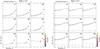 |
Fig. 7 Procrustes distance of PCA-IADI with five principal components normalized by the Procrustes distance obtained from cADI of the retrieved phase functions for different inclinations and elevations. The corresponding total field rotation is shown on the horizontal axis on top. The circles show the maximum value out of 500 iterations. The final values are shown as crosses. We note that the right panel has a different color scale from the left panel. |
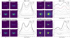 |
Fig. 8 cIADI and PCA-IADI reductions of the disk model inserted into a star with a ratio of 1 × 10⁻² (left) and 1 × 10⁻³ (right). The red dotted line is a reduction of the data set without the model inserted. The PCA-IADI reduction is done with five principal components. |
3.5 Mask and threshold
The previous section demonstrates that the introduction of a star might be detrimental to disk recovery. The effects of the star increase with decreasing S/N of the disk signal. The different effects discussed above can all be traced back to the same issue, namely that the process above is not discriminating between signal and noise for the feedback loop. In this section, the feedback of signal will be controlled via a mask and a threshold.
A binary mask can be used to indicate where the disk resides, such that only signal from where the disk should be is fed back. The mask is applied after the images have been rotated back to their original position to be subtracted from the original data set during step 6 in Fig. 1. Everything not below the mask is set to zero, such that this is not subtracted from the original set of images. While a mask can be easily generated from the model, for real observations, if available, polarimetric data of the disk can be used to generate a binary mask. However, we should note that the complete disk is not necessarily highly polarized (see e.g., Ginski et al. 2021); low scattering angles might be excluded, particularly for disks at greater inclinations. Therefore, as should be customary, a mask should be used with caution.
In the section above, all signal above zero was fed back. This includes noise, which results in generating false-positive signal and amplifying noise, which also happens within the mask. A threshold will minimize this feedback and can be implemented in addition to the mask. This threshold is dynamic, and after every iteration the threshold is calculated again. Furthermore, it depends on the distance from the star because of the star being bright at the center of the image and reducing in brightness toward the edges. Moreover, there will be more photon noise and residual speckle noise closer to the star. Hence, the standard deviation changes significantly going outward. A different standard deviation on which the threshold is based is therefore used depending on its separation from the center. This should suppress the feedback of noise even more and therefore also the generation of false-positive disk signal. The threshold system is implemented by dividing the disk into multiple annuli. For each annulus, the standard deviation of the pixel values is calculated during every iteration, and the pixels below the threshold times the standard deviation of that annulus are set to zero. For instance, for a threshold of 0.5, every value below 0.5 times the standard deviation in that annulus is set to zero.
A reduction with a threshold and a mask can be found in Fig. 9. The main difference in the left two panels of Fig. 9 compared to Fig. 8 is that, in the center of the image, the star is not fed back. This reduces the amplification of the signal in the center of the image, which means that the recovered phase function does not surpass the intensity of the phase function of the input model. The Procrustes distances of the mask and dynamic threshold reduction are lower than the reductions without. The Procrustes distance is reduced from 0.136 for the star and disk-only reduction to 0.110 with the mask and dynamic threshold implemented. This is a factor of 1.2 improvement.
Moving our attention to the 1 × l0−3 ratio reduction in the left two panels of Fig. 9, the phase function is dominated by the inner ring of the disk, a large part of which has stellar signal. When using a mask, signal from the star is still fed back, which is one of the basic problems of a mask. The threshold may help in reducing this feedback of stellar signal, but it may not reduce it completely. The Procrustes distances show that again the stellar signal is being reconstructed; after ten iterations the Procrustes distances are increasing again (from 0.180 to 0.769 for cIADI and from 1.68 to 2.14 for the five principal component PCA-IADI reduction). The reduction with no mask or dynamic threshold shows a poorer recovery than the reduction with a mask and a dynamic threshold. Lastly, the side facing the observer is clearly brighter than the other side of the disk, which originates from the original ‘pseudo’-phase function of the model.
The introduction of a mask and a dynamic threshold did reduce the creation of artefacts significantly. In all reductions with PCA-IADI and for different principal components for a ratio of 1 × 10⁻², bright rings can no longer be seen. The recovered images are clearly a better representation of the original model. However, the Procrustes distances computed are higher than without the dynamic threshold and the mask (1.68 compared to 1.07). This is mainly due to less flux being recovered around 180°, where the recovered phase function has a deeper valley than the original model. However, the signal mainly consists of disk signal instead of being dominated by the amplified noise, which is an improvement. Moreover, where first the recovered phase functions even exceeded the original model, now the dynamic threshold and mask ensure that this does not happen. We can therefore make the following conclusion: the mask and the dynamical threshold should not be used for low-S/N cases, but in the case of high S/N, they can help in recovering the disk, though they should be used with care.
4 Application to real data
4.1 HD 100546
Spiral structures have been found in the disk of HD 100546, (Avenhaus et al. 2014; Follette et al. 2017; Sissa et al. 2018; Pineda et al. 2019) and the presence of two proto-planet candidates has been proposed by several authors (Quanz et al. 2013, 2015; Currie et al. 2014, 2015), but the status of these propositions remains controversial (Garufi et al. 2016; Rameau et al. 2017). In Fig. 10, we show polarimetric and full intensity scattered light SPHERE data taken on 18 February 2019. These data were taken 30 min after meridian passing and had a duration of 2 h, resulting in 127 exposures with 34.3° of field rotation. The average field rotation between each exposure is 0.096° with a standard deviation of 0.013°, not including a large difference of 22.3° between exposures 63 and 64. This small difference between each image is due to the low elevation of the source.
The reductions of the data set are shown in Fig. 10. The polarized differential imaging result, produced with the IRDAP pipeline (van Holstein et al. 2017, 2020), is shown in the top left. The classical ADI pipeline reduction is shown in the top-center image. The reduction with PynPoint (Stolker et al. 2019) for one principal component is shown in the top-right image. For more components, the disk was completely removed. With the relatively low asymmetry of the disk in addition to the moderate amount of field rotation, Fig. 5 shows that around 300–400 iterations are sufficient to maximize the amount of flux recovered. While the disk is visible in the raw data, the ratio between the disk and the star is likely slightly poorer than shown in the left panel of Figs. 6 and 7. Therefore, approximately 300 iterations will be suitable for this dataset. In addition, the data set was processed with a mask made with the PDI image with a threshold of 20 (i.e., every pixel with a value above 20 in the PDI image is fed back) and a dynamic threshold of 0.01. The standard PCA-IADI pipeline with one principal component was used for the corresponding result, without adding a mask or dynamic threshold. The positions of the spiral and the planet candidates mentioned above are shown in the overlay.
The classical ADI result in the top-center of the image shows two structures coming from the center of the image toward the northeast. Follette et al. (2017) and others reported these features as possible spiral structures in the disk itself, with planet b positioned at the end of the top arm. However, as Garufi et al. (2016) already showed in their reductions, these are artifacts of the reduction method. Mainly the edges of the disk are recovered, and indeed with cIADI, more of the disk is recovered and none of these structures are present any longer. The recovered full intensity disk is of similar size to the disk recovered with PDI. The spiral reported by Avenhaus et al. (2014) seems to be present in the cIADI recovered image as well. No signal of any planet can be seen in the disk. The ‘dark lane’, or sharp drop in brightness in the southwest part of the disk first reported by Avenhaus et al. (2014) in polarized intensity is present here in full intensity as well.
The PynPoint reduction with one principal component shows a faintly visible disk edge at the same position as the arms in the cADI reduction. PCA-IADI does not recover as much of the disk as cIADI does. Only parts of the edges of the disk are visible. This stark difference between cIADI and PCA-IADI arises from both the amount and speed of field rotation in the data, which is only 34.3° (65% of which happens between two observations) and is constant between each image. As discussed in Sect. 3.3, PCA-IADI works best for constant field rotation with no large gaps in field rotation. On the other hand, cIADI works best for large differences in field rotation. Hence, while cIADI can recover large parts of the disk, PCA-IADI only recovers the part of the disk that changed the most during the observation.
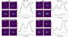 |
Fig. 9 Same reductions as in Fig. 8, but now with a mask and threshold that limit the feedback of stellar signal. |
4.2 HD 34700 A
The HD 34700 A disk consists of a large circumstellar dust ring with a major axis of 175 au (Monnier et al. 2019) to which multiple spiral arms have been found to be attached, possibly up to eight in total (Monnier et al. 2019). A discontinuity can be seen in the northern part of the dust ring as well. Figure 11 shows polarimetric and full intensity scattered light SPHERE data taken on 27 October 2019. These data were taken centered on the meridian with a duration of 1.5 h and consist of 64 exposures with 35.3° of field rotation. Each image is rotated by 0.56° on average due to field rotation. The disk is very asymmetric due to the many spirals present, which translates to a relatively high inclination in Figs. 5-7. In combination with the elevation (and amount of field rotation) the optimal number of iterations is somewhere between 100 and 200. Lastly, in the raw data, the disk is clearly visible. The disk is relatively bright compared to the star, which makes it similar to the ratio 1 × 10⁻² case discussed in Sects. 3.4 and 3.5. For these reductions, the optimal number of iterations is indeed around 200. The reductions of the data set are shown in Fig. 11. The polarized differential imaging result is shown in the top left. The classical ADI pipeline reduction is shown in the top-center image. The reduction with PynPoint for one principal component is shown in the top right image, which gave the best result compared to different numbers of principal components.
The data set was processed with cIADI for 200 iterations, together with a mask made with the PDI image with a threshold of 10, and a dynamic threshold of 0.01. The PCA-IADI pipeline with one principal component was used with the same mask and dynamic threshold as cIADI.
Figure 11 shows the position of a discontinuity in the overlay. All of the spiral arms observed by Monnier et al. (2019) can be seen in the PDI image: namely one large spiral arm on the west side of the disk extending southwest and multiple spiral arms on the north, northeast, and southeast sides of the disk. With cADI and PynPoint, the outlines of these spirals and the edges of the disk can be seen. The large extending arms are recovered well already with the classical reduction techniques thanks to their asymmetric nature. The discontinuity can be seen in these reductions as well. However, large parts of the dust ring are not recovered due to self-subtraction. With cIADI, the parts with the missing flux in the south of the disk are recovered. With PCA-IADI on the other hand, mainly the northern part of the disk is recovered. For both cases, the recovered total intensity image of the bright ring compares well with the total intensity reduction using reference differential images presented in Uyama et al. (2020) for Subaru/CHARIS data.
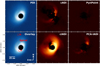 |
Fig. 10 HD 100546 reduced with different reduction techniques. The overlay shows the positions of the planet candidates (Currie et al. 2015) and the spiral arm (Avenhaus et al. 2014). |
4.3 SU Aurigae
The main feature of SU Aur is a large tail (Chakraborty & Ge 2004; Jeffers et al. 2014; de Leon et al. 2015) extending outwards to up to 1000 au on the west side of the disk. While multiple explanations for this arm have been proposed, such as a cloud remnant (Jeffers et al. 2014) or a collision with a stellar intruder (Akiyama et al. 2019), recent work by Ginski et al. (2021) shows that, by using results reported here, the tails (both the large tail in the west and the shorter one in the north) originate from still infalling material. In Fig. 12, we show the polarimetric and full intensity scattered light SPHERE data taken on 14 December 2019. The data were taken 15 min after meridian passing and took around 1 h of observation time. The data consist of 104 exposures of 32 s with a total of only 18.1° of field rotation. On average there is 0.18° of rotation in between each image. The large tail of the disk is visible in the raw data at large separations, but the disk itself is not visible.
Reductions of the data set are shown in Fig. 12. The polarized differential imaging result is shown in the top left. The classical ADI pipeline reduction is shown in the top-center image. The reduction with PynPoint for two principal components is shown in the top right image, which gave the best result compared to different numbers of principal components. The disk is very asymmetric, and therefore relatively few iterations are necessary, especially given that more noise will be produced in the process (see Fig. 4). Taking the results in Figs. 5–7 into account, the optimal number of iterations is therefore around 100. No masking has been used. The standard PCA-IADI pipeline was used with two principal components.
In the PDI image, the tails protruding to the east and west are highly visible, and the inset also shows the inner disk. Classical ADI only recovers the edges of the tails. The tail is the most asymmetric part of the disk and will show the least overlap in the data set; it will therefore also be recovered first. However, due to the small amount of field rotation and the small differences in between each image, almost nothing of the disk in the center of the image is recovered. cIADI does not help in recovering the disk itself either. The structure seen in the image is likely due to the reconstruction of the star, and its appearance is too circular to be the disk. However, the large extended tails in both the east and west directions are very well recovered. More of the structure also visible in the PDI result is now visible in the full-intensity image as well. No significant numerical rings are produced during the iteration process, even though no mask or dynamic threshold are used in this reduction.
With PynPoint, the extended tails that were also recovered with cADI can be seen here. Compared to cADI, the residual pattern changes but the disk is still not recovered. PCA-IADI recovers more of the tail. As with cIADI, both the eastern and western tails are filled in due to the iteration process. The northern part of the westward protruding tail is much brighter than with PDI. However, due to the iteration process, the numerical rings are amplified by the PCA-IADI reduction (as was expected from Sects. 3.3 and 3.4). Hence, cIADI would be better suited for this disk.
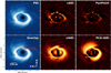 |
Fig. 11 HD 34700 A reduced with different reduction techniques. The overlay shows the discontinuity as found by Monnier et al. (2019). |
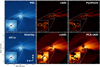 |
Fig. 12 SU Aurigae reduced with different reduction techniques. |
5 Summary
In Sect. 3.3 we present our assessment of the effectiveness and efficiency of two different algorithm versions of IADI: classical Iterative Angular Differential Imaging (cIADI), which determines the PSF of the star via taking the median of the data set, and principal component analysis-iterative differential imaging (PCA-IADI), which determines the PSF of the star via PCA (identical to the GreeDS algorithm presented by Pairet et al. 2021). Processing is performed for model-only and star+model cases. Here we provide a short summary of our findings and present our main conclusions.
Asymmetries are an important factor in recovering the disk. These asymmetries can either be caused by the inherent structure of the disk, or by the inclination of the disk. With less of the disk overlapping in the data set, more of the disk is recovered. The other important factor in recovering the disk is the amount of field rotation caused by the declination of the disk and latitude of the telescope, that is, the elevation of the disk. In general, with more field rotation, more of the disk is recovered because of a reduction in the overlap between images. However, the speed with which the field rotation occurs is important as well. The higher the elevation, the faster the rotation happens. Consequently, most of the images in the data set will appear similar because most of the rotation happens only between a few of the images in the data set. Which is a well-established behavior of all ADI algorithms. For IADI on the other hand, different behaviors are seen for different speeds of field rotation. cIADI works best for data sets containing high amounts of field rotation, while PCA-IADI works better with data sets containing evenly rotated images. When the images are evenly rotated, the difference between every single image is maximal which gives PCA-IADI the best opportunity to distinguish the disk from the stellar PSF in the data set.
Keeping these limitations in mind, we find that both variations of IADI significantly increase the recovered disk flux in the model-only processed data sets. The throughput is close to 100% for disks with high inclination (i > 75°) and pass meridian within ~10° of the local zenith. Even for the worst case of a nearly face-on disk (i = 5°), a ~20% throughput is achieved assuming that the target passes meridian within ~ 15° of the local zenith. For the Paranal observatory, this requirement would be fulfilled for several of the abundant nearby star-forming regions, such as the Lupus cloud complex or Corona Australis.
For cIADI, the disk is best recovered in the high-flux-ratio case, but the star still introduces asymmetries into the recovered phase functions. For PCA-IADI, depending on the number of principal components used, numerical artifacts were made worse or were completely removed. In general, the application of PCA-IADI led to reduced throughput but also reduced stellar noise. However, for the low-flux-ratio case, the recovered phase functions were dominated by stellar speckle noise in both techniques. By applying the Procrustes metric, we find that, depending on the flux ratio, a small number of iterations (~10) is optimal, because the stellar speckle halo tends to be dominantly reconstructed at higher iterations. The mask and dynamic threshold do significantly improve the recovery of the disk as well as the phase function, especially in the 1 × 10⁻³ ratio case for cIADI. For PCA-IADI, the masking technique may introduce false-positive signal for disks with low flux ratios and should be applied cautiously.
For the three exemplary cases of observed disks, a significant improvement is made on the recovery of the disk in full-intensity NIR scattered light. While with previously used techniques, such as classical ADI and PynPoint, only the edges of the disks or spiral arms were recovered, IADI increases throughput for the inner disk and specifically low-spatial-frequency signal. This is also what is found in the theoretical part of this work; the model disks were always recovered from the edges inward, filling in the self-subtracted regions. The best example of this is HD 100546, only the edges of which were recovered with cADI (and PynPoint), but with cIADI the disk is reconstructed from these edges inward resulting in a more complete recovery of the disk in full-intensity scattered light. These edges were recovered previously (e.g., Currie et al. 2015; Garufi et al. 2016; Rameau et al. 2017), and some were interpreted as real features of the disk. Therefore, these interpretations need to be reconsidered thoroughly, because some of these might be artifacts of the ADI method used. While none of the disks are very symmetric, extended features such as long spiral arms were recovered in greater detail than for example the central regions of the disk. This can be seen in SU Aur, which consists of both a symmetric inner disk and a large westward extending arm. While the arm is recovered in similar detail to the result from PDI, the inner region of the disk is not. Another example is HD 34700 A, where the spiral arms visible in PDI can be seen in classical ADI or PynPoint, but not with as much detail. IADI (either classical or PCA based) recovered the spiral arms well due to their asymmetric nature.
One of the main difficulties with IADI is the generation and amplification of noise. In Sect. 3.4, this manifested in ring structures due to both the intrinsic noise of the image and the signal coming from the star being smeared out into circles because of the interpolation used for rotating the images during the iterative process. PCA-IADI amplified these noise-induced ring structures even more by fitting them in the PCA-subtraction process. This causes the noise amplification to be greater with PCA-IADI than with cIADI. However, this depends on how bright the disk is compared to the star. For the reductions of real measurements, most disks were relatively bright when compared to the star (close to the theoretical 1 × 10⁻² flux ratio case). The further away from the star, the less of a problem these artifacts become. This can be seen in the reduction of SU Aur. Here, the rings are likely generated from interpolation artifacts, while closer in to the star the residual speckle noise causes the ring structures. The PCA-IADI reduction of SU Aur revealed more rings than the cIADI reduction. As is found in Sect. 3.4 as well, PCA-IADI amplifies the noise much more than cIADI, which is clear from this latter reduction as well.
In conclusion, IADI indeed improves the recovery of the disk in full-intensity NIR scattered light significantly compared to the standard ADI algorithms. After post-processing, in many cases the disk is as well recovered as with PDI. Many of the features visible with PDI are also visible with IADI. However, IADI still has to cope with some problems. The amplification and generation of (numerical and/or correlated) noise is still an issue that has to be dealt with. In the mean time, IADI can work very well for disks that are relatively bright and extended.
Acknowledgements
SPHERE is an instrument designed and built by a consortium consisting of IPAG (Grenoble, France), MPIA (Heidelberg, Germany), LAM (Marseille, France), LESIA (Paris, France), Laboratoire Lagrange (Nice, France), INAF—Osservatorio di Padova (Italy), Observatoire de Genève (Switzerland), ETH Zurich (Switzerland), NOVA (Netherlands), ONERA (France), and ASTRON (The Netherlands) in collaboration with ESO. SPHERE was funded by ESO, with additional contributions from CNRS (France), MPIA (Germany), INAF (Italy), FINES (Switzerland), and NOVA (The Netherlands). SPHERE also received funding from the European Commission Sixth and Seventh Framework Programmes as part of the Optical Infrared Coordination Network for Astronomy (OPTICON)under grant No. RII3-Ct2004-001566 for FP6 (2004-2008), grant No. 226604 for FP7 (2009-2012), and grant No. 312430 for FP7 (2013-2016). This work makes use of the following software: Python version 3.9, astropy (Astropy Collaboration 2013, 2018), matplotlib (Hunter 2007), numpy (Harris et al. 2020), opencv (Bradski 2000), pynpoint (Stolker et al. 2019), scipy (Virtanen et al. 2020). Lastly, we thank an anonymous referee for their careful consideration of our work and for their thoughtful comments which significantly improved the manuscript.
Appendix A Field Rotation for Different Declinations and Latitudes
Figure A.1 presents the amount of field rotation for different latitudes of the telescope and declinations of the target. When the declination and latitude are the same, the elevation is 90° and the object has a total of 180° of field rotation, which reduces for lower elevations. In most cases, the amount of field rotation for different elevations is the same, especially for the major direct imaging facilities. For high latitudes, the amount of field rotation reduces. Therefore, in the case of high latitudes, the results shown in this work are optimistic because of the much reduced field rotation. However, at these high latitudes, ADI in general would be inefficient.
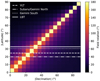 |
Fig. A.1 Absolute latitude of the telescope vs. absolute declination of the object. The colors represent the total amount of field rotation for a one-hour observation. The lines are the latitudes of the major direct imaging facilities. |
References
- Akiyama, E., Vorobyov, E. I., Baobabu Liu, H., et al. 2019, AJ, 157, 165 [Google Scholar]
- Amara, A., & Quanz, S. P. 2012, MNRAS, 427, 948 [Google Scholar]
- Apai, D., Pascucci, I., Brandner, W., et al. 2004, A&A, 415, 671 [NASA ADS] [CrossRef] [EDP Sciences] [Google Scholar]
- Astropy Collaboration (Robitaille, T. P., et al.) 2013, A&A, 558, A33 [NASA ADS] [CrossRef] [EDP Sciences] [Google Scholar]
- Astropy Collaboration (Price-Whelan, A. M., et al.) 2018, AJ, 156, 123 [Google Scholar]
- Avenhaus, H., Quanz, S. P., Meyer, M. R., et al. 2014, ApJ, 790, 56 [Google Scholar]
- Avenhaus, H., Quanz, S. P., Schmid, H. M., et al. 2017, AJ, 154, 33 [Google Scholar]
- Avenhaus, H., Quanz, S. P., Garufi, A., et al. 2018, ApJ, 863, 44 [NASA ADS] [CrossRef] [Google Scholar]
- Benisty, M., Juhász, A., Facchini, S., et al. 2018, A&A, 619, A171 [NASA ADS] [CrossRef] [EDP Sciences] [Google Scholar]
- Benisty, M., Dominik, C., Follette, K., et al. 2022, ApJ, submitted [arXiv:2203.09991] [Google Scholar]
- Beuzit, J. L., Vigan, A., Mouillet, D., et al. 2019, A&A, 631, A155 [NASA ADS] [CrossRef] [EDP Sciences] [Google Scholar]
- Bradski, G. 2000, The OpenCV Library, Dr. Dobb’s Journal of Software Tools [Google Scholar]
- Chakraborty, A., & Ge, J. 2004, AJ, 127, 2898 [NASA ADS] [CrossRef] [Google Scholar]
- Chauvin, G., Desidera, S., Lagrange, A. M., et al. 2017, A&A, 605, L9 [NASA ADS] [CrossRef] [EDP Sciences] [Google Scholar]
- Currie, T., Muto, T., Kudo, T., et al. 2014, ApJ, 796, L30 [Google Scholar]
- Currie, T., Cloutier, R., Brittain, S., et al. 2015, ApJ, 814, L27 [Google Scholar]
- de Boer, J., Salter, G., Benisty, M., et al. 2016, A&A, 595, A114 [NASA ADS] [CrossRef] [EDP Sciences] [Google Scholar]
- de Leon, J., Takami, M., Karr, J. L., et al. 2015, ApJ, 806, L10 [Google Scholar]
- Dryden, I. L., & Mardia, K. V. 2016, Statistical Shape Analysis: with Applications in R (Hoboken: John Wiley & Sons), 995 [Google Scholar]
- Follette, K. B., Rameau, J., Dong, R., et al. 2017, AJ, 153, 264 [Google Scholar]
- Garufi, A., Quanz, S. P., Schmid, H. M., et al. 2016, A&A, 588, A8 [NASA ADS] [CrossRef] [EDP Sciences] [Google Scholar]
- Ginski, C., Stolker, T., Pinilla, P., et al. 2016, A&A, 595, A112 [NASA ADS] [CrossRef] [EDP Sciences] [Google Scholar]
- Ginski, C., Facchini, S., Huang, J., et al. 2021, ApJ, 908, L25 [NASA ADS] [CrossRef] [Google Scholar]
- Harris, C. R., Millman, K. J., van der Walt, S. J., et al. 2020, Nature, 585, 357 [NASA ADS] [CrossRef] [Google Scholar]
- Hunter, J. D. 2007, Comput. Sci. Eng., 9, 90 [NASA ADS] [CrossRef] [Google Scholar]
- Jeffers, S. V., Min, M., Canovas, H., Rodenhuis, M., & Keller, C. U. 2014, A&A, 561, A23 [NASA ADS] [CrossRef] [EDP Sciences] [Google Scholar]
- Kuhn, J. R., Potter, D., & Parise, B. 2001, ApJ, 553, L189 [NASA ADS] [CrossRef] [Google Scholar]
- Lafrenière, D., Marois, C., Doyon, R., Nadeau, D., & Artigau, É. 2007, ApJ, 660, 770 [Google Scholar]
- Laws, A. S. E., Harries, T. J., Setterholm, B. R., et al. 2020, ApJ, 888, 7 [Google Scholar]
- Macintosh, B., Graham, J. R., Ingraham, P., et al. 2014, Proc. Natl. Acad. Sci., 111, 12661 [NASA ADS] [CrossRef] [Google Scholar]
- Macintosh, B., Graham, J. R., Barman, T., et al. 2015, Science, 350, 64 [Google Scholar]
- Marois, C., Lafrenière, D., Doyon, R., Macintosh, B., & Nadeau, D. 2006, ApJ, 641, 556 [Google Scholar]
- Marois, C., Macintosh, B., Barman, T., et al. 2008, Science, 322, 1348 [Google Scholar]
- Marois, C., Zuckerman, B., Konopacky, Q. M., Macintosh, B., & Barman, T. 2010, Nature, 468, 1080 [NASA ADS] [CrossRef] [Google Scholar]
- Milli, J., Mouillet, D., Lagrange, A. M., et al. 2012, A&A, 545, A111 [NASA ADS] [CrossRef] [EDP Sciences] [Google Scholar]
- Min, M., Hovenier, J. W., & de Koter, A. 2005, A&A, 432, 909 [NASA ADS] [CrossRef] [EDP Sciences] [Google Scholar]
- Monnier, J. D., Harries, T. J., Bae, J., et al. 2019, ApJ, 872, 122 [Google Scholar]
- Murakawa, K. 2010, A&A, 518, A63 [NASA ADS] [CrossRef] [EDP Sciences] [Google Scholar]
- Muro-Arena, G. A., Benisty, M., Ginski, C., et al. 2020, A&A, 635, A121 [NASA ADS] [CrossRef] [EDP Sciences] [Google Scholar]
- Pairet, B., Cantalloube, F., & Jacques, L. 2018, ArXiv e-prints [arXiv:1812.01333] [Google Scholar]
- Pairet, B., Cantalloube, F., & Jacques, L. 2021, MNRAS, 503, 3724 [Google Scholar]
- Perrot, C., Boccaletti, A., Pantin, E., et al. 2016, A&A, 590, L7 [NASA ADS] [CrossRef] [EDP Sciences] [Google Scholar]
- Pineda, J. E., Szulágyi, J., Quanz, S. P., et al. 2019, ApJ, 871, 48 [Google Scholar]
- Pohl, A., Benisty, M., Pinilla, P., et al. 2017, ApJ, 850, 52 [Google Scholar]
- Quanz, S. P., Amara, A., Meyer, M. R., et al. 2013, ApJ, 766, L1 [Google Scholar]
- Quanz, S. P., Amara, A., Meyer, M. R., et al. 2015, ApJ, 807, 64 [Google Scholar]
- Rameau, J., Follette, K. B., Pueyo, L., et al. 2017, AJ, 153, 244 [Google Scholar]
- Ren, B., Pueyo, L., Zhu, G. B., Debes, J., & Duchêne, G. 2018, ApJ, 852, 104 [Google Scholar]
- Sissa, E., Gratton, R., Garufi, A., et al. 2018, A&A, 619, A160 [NASA ADS] [CrossRef] [EDP Sciences] [Google Scholar]
- Stolker, T., Dominik, C., Avenhaus, H., et al. 2016, A&A, 595, A113 [NASA ADS] [CrossRef] [EDP Sciences] [Google Scholar]
- Stolker, T., Min, M., Stam, D. M., et al. 2017, A&A, 607, A42 [NASA ADS] [CrossRef] [EDP Sciences] [Google Scholar]
- Stolker, T., Bonse, M. J., Quanz, S. P., et al. 2019, A&A, 621, A59 [NASA ADS] [CrossRef] [EDP Sciences] [Google Scholar]
- Tazaki, R., Tanaka, H., Muto, T., Kataoka, A., & Okuzumi, S. 2019, MNRAS, 485, 4951 [NASA ADS] [CrossRef] [Google Scholar]
- Uyama, T., Currie, T., Christiaens, V., et al. 2020, ApJ, 900, 135 [NASA ADS] [CrossRef] [Google Scholar]
- van Boekel, R., Henning, T., Menu, J., et al. 2017, ApJ, 837, 132 [Google Scholar]
- van Holstein, R. G., Snik, F., Girard, J. H., et al. 2017, SPIE Conf. Ser., 10400, 1040015 [Google Scholar]
- van Holstein, R. G., Girard, J. H., de Boer, J., et al. 2020, A&A, 633, A64 [NASA ADS] [CrossRef] [EDP Sciences] [Google Scholar]
- van Holstein, R. G., Stolker, T., Jensen-Clem, R., et al. 2021, A&A, 647, A21 [EDP Sciences] [Google Scholar]
- Virtanen, P., Gommers, R., Oliphant, T. E., et al. 2020, Nat. Methods, 17, 261 [Google Scholar]
- Wang, J. J., Ruffio, J.-B., De Rosa, R. J., et al. 2015, Astrophysics Source Code Library [record ascl:1506.001] [Google Scholar]
We note that in both cases we use the full science data set for the median combination as well as the PCA; i.e., we did not implement an “exclusion angle” as is done in some cases to limit self-subtraction (e.g., LOCI Lafrenière et al. 2007; pyKLIP Wang et al. 2015).
We note that flatter disk profiles were recovered by Avenhaus et al. (2018) for several T Tauri stars, which would lead to a slightly smaller offset of the disk rings from the stellar position.
All Figures
|
Fig. 1 Flowchart depicting the different steps in the IADI reduction process. 0. Copy of the original data set, which is used after every iteration. 1. The original data set minus the final result from step 5. If this is the first iteration, the data sets of step 0 and 1 are identical. Even after some iterations, some disk signal is left in this data set after subtracting the final result. This is shown as the gray dotted ellipses. 2. Take the median of the data set (cIADI) or construct the PSF with principal components after taking the mean of the data set (PCA-IADI). 3. Subtract the found PSF from each image in the original data set copied in step 0. 4. Derotate the data set such that the science object has the same orientation in all images. 5. Take the median of all derotated images to combine them and get the final result. 6. Feedback all positive signal of the final result from step 5 to step 1 and then repeat the process. |
| In the text | |
|
Fig. 2 Model used in this work together with a reduction with the IADI pipeline. The top panels show, from left to right, a ~1/r2 intensity dependence from the center of the disk, the addition of the phase function, and telescope resolution. The bottom panels present the recovered disk after 1, 100, and 1000 iterations. This shows that with classical ADI, large parts of the disk are not recovered due to self-subtraction, but that these can be recovered iteratively. All images use a log-scale to make the faint parts of the disk more visible. |
| In the text | |
|
Fig. 3 Recovered flux, numerical noise, and corrected flux plotted against the number of iterations of a disk with an inclination of 45° and elevation of 85° processed with cIADI. Both spline interpolation (dashed lines) and nearest-neighbor interpolation (continuous lines) are shown. |
| In the text | |
|
Fig. 4 Recovered flux and generated numerical noise with cIADI and PCA-IADI after 500 iterations for a grid of models with different inclinations and elevations. The corresponding amount of field rotation is indicated by the vertical axis on the right. The top row shows the recovered flux and the bottom row the numerical noise. The rightmost column shows the difference between PCA-IADI and cIADI. |
| In the text | |
|
Fig. 5 Number of iterations necessary to reach 99% of the flux recovered after 500 iterations; i.e., the convergence speed. |
| In the text | |
|
Fig. 6 Procrustes distance of cIADI normalized by the Procrustes distance obtained from cADI of the retrieved phase functions for different inclinations and elevations. The corresponding total field rotation is shown on the horizontal axis on top. The circles show the maximum value out of 500 iterations. The final values are shown as crosses. We note that the right panel has a different color scale from the left panel. |
| In the text | |
|
Fig. 7 Procrustes distance of PCA-IADI with five principal components normalized by the Procrustes distance obtained from cADI of the retrieved phase functions for different inclinations and elevations. The corresponding total field rotation is shown on the horizontal axis on top. The circles show the maximum value out of 500 iterations. The final values are shown as crosses. We note that the right panel has a different color scale from the left panel. |
| In the text | |
|
Fig. 8 cIADI and PCA-IADI reductions of the disk model inserted into a star with a ratio of 1 × 10⁻² (left) and 1 × 10⁻³ (right). The red dotted line is a reduction of the data set without the model inserted. The PCA-IADI reduction is done with five principal components. |
| In the text | |
|
Fig. 9 Same reductions as in Fig. 8, but now with a mask and threshold that limit the feedback of stellar signal. |
| In the text | |
|
Fig. 10 HD 100546 reduced with different reduction techniques. The overlay shows the positions of the planet candidates (Currie et al. 2015) and the spiral arm (Avenhaus et al. 2014). |
| In the text | |
|
Fig. 11 HD 34700 A reduced with different reduction techniques. The overlay shows the discontinuity as found by Monnier et al. (2019). |
| In the text | |
|
Fig. 12 SU Aurigae reduced with different reduction techniques. |
| In the text | |
|
Fig. A.1 Absolute latitude of the telescope vs. absolute declination of the object. The colors represent the total amount of field rotation for a one-hour observation. The lines are the latitudes of the major direct imaging facilities. |
| In the text | |
Current usage metrics show cumulative count of Article Views (full-text article views including HTML views, PDF and ePub downloads, according to the available data) and Abstracts Views on Vision4Press platform.
Data correspond to usage on the plateform after 2015. The current usage metrics is available 48-96 hours after online publication and is updated daily on week days.
Initial download of the metrics may take a while.