© The Authors 2023

1 Introduction

Direct imaging is an observational method that is particularly adapted to the detection and characterization of young giant exoplanets orbiting nearby stars (Traub et al. 2010). It requires us to reach a high contrast and a high angular resolution through a combination of (i) cutting-edge observational facilities, (ii) custom observational techniques, and (iii) advanced (post)-processing algorithms. Concerning instrumental aspects, the main ground-based observatories are now equipped with dedicated instruments (e.g., Gemini/GPI, Macintosh et al. 2008; Keck/NIRC2, Xuan et al. 2018; Magellan/MagAO-X, Close et al. 2018; VLT/SPHERE, Beuzit et al. 2019; Subaru/SCExAO, Jovanovic et al. 2015) that integrate an extreme adaptive system and a coronagraphic mask to cancel out most of the stellar light. In spite of these cutting-edge facilities, the observations stay dominated by a strong and spatially correlated stellar nuisance, which is an obstacle to the detection of objects of interest. This nuisance component is formed by the additive contribution of the so-called speckles and of other sources of noise (i.e., thermal background, detector readout, and photon noise). Speckles are stellar leakages impacted by diffraction effects in the presence of residual (uncorrected) aberrations and currently remain the main source of limitation to the achievable contrast (Soummer et al. 2007; Bailey et al. 2016). In that context, observations are usually conducted with custom techniques in order to bring additional sources of diversity (e.g., temporal, spectral, polarimetric) to unmix the contribution of the sought-for objects from that of the nuisance. In this paper, we focus on angular differential imaging (ADI; Marois et al. 2006) in combination with spectral differential imaging (SDI; Racine et al. 1999). The ADI process brings on a temporal diversity by using the pupil-tracking mode of the telescope, so that speckles remain quasi-static across exposures, while the objects of interest follow a circular rotation with respect to the star. This apparent motion is deterministic and depends solely on the experienced parallactic rotation angles. Then, SDI guarantees spectral diversity by simultaneously recording images in several spectral channels using an integral field spectrograph (IFS) or a dual band imager (IRDIS) with less spectral leverage.

A large variety of post-processing algorithms has been developed in the last decade to extract the relevant information from 3D (respectively, 4D) datasets recorded by ADI (respectively, ASDI), see e.g., Pueyo (2018); Cantalloube et al. (2020) for reviews. Among these methods, the PACO algorithm (Flasseur et al. 2018, 2020a,b) has been shown to be particularly efficient for the processing of A(S)DI observations. It statistically captures the spatio-temporo-spectral correlations of the data with a weighted multi-variate Gaussian model whose parameters are estimated, in a data-driven fashion, at the scale of a patch of a few tens of pixels. With VLT/SPHERE observations where the typical spatial correlation scale of speckles lies in a few tens of pixels, Flasseur et al. (2018, 2020a,b); Cantalloube et al. (2020) and Chomez et al. (2023) showed that this parameterfree method provides an improved detection sensitivity with respect to the baseline processing methods of the field (i.e., cADI Marois et al. 2006, TLOCI Marois et al. 2014 and KLIP Soummer et al. 2012, as well as Amara & Quanz 2012). It also provides reliable estimates of the detection confidence and of the astro-photometry with the associated uncertainties.

Whatever the chosen post-processing algorithm, detection performance stay upper-bounded by the lack of diversity at short angular separation, where (i) the speckle field is dominant and displays the largest temporal fluctuations and (ii) the apparent displacement of the objects of interest induced by A(S)DI is not sufficient to extract their signals without bias. From a data science point of view, two main avenues are currently investigated to mitigate these limitations. The first category of methods targets a better elimination of the nuisance component. It usually consists of building a finer model of the stellar (on-axis) point spread function (PSF). This model can be built from several datasets, resulting from the observation of different stars, in which the objects of interest are not expected to be co-localized. This is the general principle of approaches based on reference differential imaging (Ruane et al. 2019; Wahhaj et al. 2021; Sanghi et al. 2022; Xie et al. 2022). The second category of methods targets a better combination of the signal of the objects of interest. It consists of combining several epochs¹ to constructively co-add their signal by taking into account their proper Keplerian orbital motion. In the following, we focus on this second category of approaches, as it is more relevant to the algorithm presented in this paper.

The idea of exploiting several observations of the same star is a quite standard approach (e.g., in planetology for the detection of faint asteroid’s satellites, Marchis et al. 2005; Berdeu et al. 2022) and it is not novel in the field exoplanet characterization by direct imaging. As an illustration, the evaluation (e.g., based on system stability criteria) of the exoplanet orbits are routinely performed by fitting their previously extracted astrometry at each individual epoch with dedicated algorithms (Blunt et al. 2020). In the same vein, Skemer & Close (2011) proposed “de-orbitizing” detection maps from different epochs, namely, to transform plus re-scale each map by compensating for the orbital motion of known companions based on ephemeris calculus. This pragmatic approach, based on a prior information about the source orbits, allows to re-detect them with an improved signal-to-noise ratio (S/N), which is useful for their characterization but remains blind to unknown candidates. From a theoretical point of view, Males et al. (2013) studied the effect of the orbital motion on the detection sensitivity. They showed that orbital motion is difficult to exploit to reach 10⁻⁶ to 10⁻⁷ contrasts at small separations (typically, 0.1″ to 0.5″) currently needed in the search for Jupiter-like exoplanets by a multi-epoch combination of the data from the existing ten meters class telescopes. Proper orbital modeling will be even more crucial in the context of the quest of Neptune-like and Earth-like exoplanets with the thirty meters class telescopes (e.g., ELT, TMT, GMT). Indeed, the deep exploration of the inner environment (typically located at a few au) of the nearby solar-type stars will require contrasts of up to 10⁻⁸ to 10⁻⁹, implying long exposure times of possibly several tens of hours, which can only be achieved by conducting several observations split over several days, weeks, or months. For such observations, the orbital motion of exoplanets is not negligible at timescales of a few days or weeks. Combining the resulting multi-epoch observations without compensating for the Keplerian orbital motion will lead to a drastic degradation of the detection confidence, thus strongly limiting the achievable contrast, even for epochs separated from few weeks to few days. In that context, Males et al. (2015) suggested that orbital differential imaging (ODI), namely, the combination of multi-epoch observations with a proper compensation of the orbital motion of point-like sources, can bring an additional diversity, complementary to A(S)DI, in order to unmix the signal of very faint objects from the nuisance component. However, Males et al. (2015) also emphasized that ODI requires a dedicated (statistical) framework since the application of detection metrics commonly used in the direct imaging community for single-epoch analysis leads to a false alarm rate that is significantly higher than expected – and even more so when multiplying the number of (possibly quite similar) tested orbits. This precludes the application of their approach to blind searches, namely, those conducted without prior information about the orbit and/or about tight distributions of the orbital elements (e.g., obtained with other observational techniques), similarly to the Proxima Centauri b search from Gratton et al. (2020). The K-Stacker algorithm (Le Coroller et al. 2015, 2020, 2022; Nowak et al. 2018), also used in this latter work, is the first method addressing multi-epoch staking for blind search of exoplanets in direct imaging at high contrast. It combines (i) a brute-force step testing a large amount of orbits pre-defined on a grid, with (ii) a local refinement of the best orbits from the first step by gradient-descent optimization. K-Stacker is able to detect point-like sources that remain undetectable in each individual epoch, without any knowledge or strong priors on the source’s orbits. The algorithm also delivers, as a byproduct, an estimate of the orbital elements of the detected sources. Very recently, Thompson et al. (2023) proposed an alternative to K-Stacker integrating: (i) a dynamic orbit sampler based on Markov chain Monte Carlo (MCMC) and (ii) a joint probabilistic model of the orbit and of a common photometry consistent across epochs. Integrating this model in a Bayesian framework and marginalizing over all the orbital elements allows to derive metrics to evaluate the significance of a detection. Besides, an estimate of the orbit uncertainties can be derived from the underlying posterior distributions. The idea of combining multi-epoch direct imaging data with other methods was also studied. For e Eridani b, Mawet et al. (2019) made use of direct imaging data and radial velocity (RV) measurements to constrain the orbital elements of the planet historically confirmed via astrometry. This idea was later carried and improved by Llop-Sayson et al. (2021), who added astrometric measurements to the two other methods. They showed that even if not direct imaging detection were made alone, combining it with astrometry and RVs consequently helped constraining the orbit of e Eridani b.

For all these multi-epoch combination algorithms, the detection sensitivity and the astrophysical interpretability of the estimates are limited. A major drawback is related to the use (as input) of individual residual images (i.e., those constructed from the subtraction of an estimation of the on-axis PSF) produced by standard single-epoch algorithms (e.g., based on a principal component analysis, Soummer et al. 2012; Amara & Quanz 2012) that are known to reach moderate detection sensitivities and that are prone in some cases to a large number of false alarms especially near the star (e.g., see Flasseur et al. 2018, 2020a; Cantalloube et al. 2020; Chomez et al. 2023). These issues are even more problematic since the inner star environment corresponds to the area where the room for improvement with respect to a single-epoch analysis is the most substantial. These side effects are the direct consequence of the absence of explicit modeling of the non-stationarity and of the multiple correlations (spatial, temporal, or spectral) of A(S)DI observations. In addition, most existing multi-epoch combination algorithms lack a dedicated statistical framework to properly propagate the single-epoch uncertainties. As a result, combined multi-epoch metrics (i.e., detection confidence, achievable contrast, orbital elements, etc.) cannot be fully interpreted as strict measures. Another important source of limitation is related to the photometric calibration of the datasets. Most of the algorithms assume that the companion’s relative photometry (i.e., contrast) is constant across epochs, while it is well known that this is a critical issue in direct imaging (Biller et al. 2021). The sources of relative photometric variability are multiple: evolution of the companion’s angular separation and its associated biases, instrumental calibration issues, variability of the atmospheric conditions, and (only marginally) the intrinsic variability of the companion brightness. This strong assumption leads to some loss of sensitivity and can even lead to an increase of the false alarm rate in the multi-epoch combination. Most advanced algorithms cope with these different issues only partially by resorting to empirical, and possibly time consuming, correction steps: for instance, by filtering, massive injections of synthetic exoplanets, annular corrections of the estimated detection confidence by the variance of the flux maps, and via small-sample statistics (Mawet et al. 2014). Once again, these additional processing steps ignore the complex non-stationarity and the multiple correlations of the data. In that context, the analysis of multi-epoch results lacks of automaticity and often requires the close inspection of the combined detection maps by an expert, whose judgement remains subject to interpretation. The numerous candidate companions (e.g., around β Pictoris, Le Coroller et al. 2020; HD 95086, Le Coroller et al. 2020; Desgrange et al. 2022; α Centauri A, Le Coroller et al. 2022; HR 8799 Thompson et al. 2023) targeted by multi-epoch algorithms and that currently remain unconfirmed is a crude illustration of this lack of statistically grounded measures in the field.

Based on the analysis of the current limitations of existing multi-epoch combination algorithms, we list some requirements for a new approach, namely: (i) achieving an improved detection sensitivity; (ii) deriving interpretable combined metrics (i.e., detection scores interpretable in terms of probability of detection and of probability of false alarm, as well as reliable estimates of the orbits and of the associated error bars) by a end-to-end propagation of the uncertainties; (iii) remaining robust to the highly variable quality of each individual epoch and to the lack of absolute calibration of the relative photometric variability across epochs; and (iv) integrating some prior domain knowledge in the form either of additional parameters to be optimized (e.g., common stellar mass) or of additional constraints (e.g., known system resonances, when available). The method we propose in this paper², dubbed PACOME (for PACO Multi-Epoch)³, specifically addresses these points by capitalizing on the statistical framework of the PACO algorithm dedicated to the post-processing of single-epoch datasets. Rather than directly using the outputs of PACO as inputs of PACOME, we extend the statistical formalism of PACO for optimal multi-epoch combination of A(S)DI observations by accounting for the Keplerian orbital motion of the sought-for objects. This new framework maximizes the likelihood of the observations given its underlying model.

This paper is organized as follows. Section 2 formalizes the statistical framework we derived for multi-epoch combination. Section 3 presents the practical algorithm we propose by combining the multi-epoch statistical framework with an exploration of the possible orbits of the sought-for objects. Section 4 assesses the performance of PACOME on A(S)DI observations from the VLT/SPHERE instrument, both by resorting to injections of synthetic exoplanets and by considering a study-case example on the HR 8799 system. Finally, Sect. 5 concludes this paper and suggests a number of future prospects.

2 Multi-epoch combination formalism

Throughout this section (and when possible throughout the paper), the algorithm is described in a general fashion considering ASDI observations, without any explicit differentiation between ADI and ASDI. The formalism remains valid for ADI observations by downgrading the model to a single spectral channel without any loss of generality.

2.1 Direct model of the observations

Classical ASDI datasets are temporal sequences of corona-graphic images, decoupled into spectral channels and recorded at different epochs. The apparent position on the sky θ_t(μ) of a (point-like) celestial body following a Keplerian motion depends on a set of orbital elements μ and on the epoch of observation t. We model a N-pixel observed intensity image, r_t,ℓ,k ∈ ℝ^N, taken at epoch, t, spectral channel, ℓ, and temporal frame, k, via: $$r_{t,\ell ,k}={\alpha }_{t,\ell }{h}_{t,\ell }\left({\theta }_t\left(\mu \right)\right)+f_{t,\ell ,k},$$(1)

with θ_t (μ) as the 2D angular location of the companion at epoch, t, for a given set of orbital elements, μ, h_t,ℓ(θ) ∈ ℝ^N, the off-axis PSF centered at angular location, θ, and identical for all frames, k, of the same epoch, α_t,ℓ as the contrast of the companion⁴ at epoch, t, and spectral channel, ℓ, and f_t,ℓ,k as a nuisance term representing all other contributions other than the mean signal due to the companion. The nuisance term notably accounts for the stellar leakages, as well as for the thermal background for the sources of noise such as detector readout noise and photon noise. The main notations used in this paper are summarized in Table 1.

Given the number of photons collected by any pixel of the detector is sufficient, a weighted multi-variate Gaussian distribution has been shown to be a good approximation for the nuisance term (Flasseur et al. 2018, 2020a,b). However, when the scale of the spatial (or spectral) correlations is larger than a few tens of pixels (as may occur near the coronagraph or with broad band observations), this approximation does not hold perfectly (see Sect. 4.5.3 for a discussion of this effect). Images in different spectral channels and/or epochs are mutually independent and nearly identically distributed for a given epoch and spectral channel: $$f_{t,\ell ,k}\sim 𝒩\left({\overline{f}}_{t,\ell },{\sigma }_{t,\ell ,k}^2{C}_{t,\ell }\right),$$(2)

with ${\overline{f}}_{t,\ell }$ and C_t,ℓ as the expectation and the typical covariance matrix of the nuisance term, f_t,ℓ,_k, and where ${\sigma }_{t,\ell ,k}^2$ are the temporo-spectral correction factors accounting for the uneven quality of the frames (Flasseur et al. 2020a).

2.1.1 Maximum likelihood estimation

Extending the PACO formalism (Flasseur et al. 2018, 2020a,b) to multi-epoch ASDI observations, the total log-likelihood of the data results from the statistical model assumed in Eq. (2) for the nuisance term: $$\begin{array}{l}ℒ\left(\alpha ,\mu ,\overline{f},\sigma ,C\right)={\displaystyle \sum _{t,\ell ,k}\log p\left(r_{t,\ell ,k}|{\alpha }_{t,\ell ,}\mu \right)}\hfill \\ ={\text{c}}_1-\frac{1}{2}{\displaystyle \sum _{t,\ell ,k}\log \det \left({\sigma }_{t,\ell ,k}^2{C}_{t,\ell }\right)}\hfill \\ -\frac{1}{2}{\displaystyle \sum _{t,\ell ,k}{\Vert r_{t,\ell ,k}-{\alpha }_{t,\ell }{h}_{t,\ell }\left({\theta }_t\left(\mu \right)\right)-{\overline{f}}_{t,\ell }\Vert }_{{\sigma }_{t,\ell ,k}^{-2}{C}_{t,\ell }^{-1}}^2,}\hfill \end{array}$$(3)

where c₁ is an irrelevant constant and ${\Vert x\Vert }_A^2=x^{\text{⊤}}Ax$ denotes the squared Mahalanobis norm of x.

The maximum likelihood estimation of ${\overline{f}}_{t,\ell }$, C_t,ℓ, and ${\sigma }_{t,\ell ,k}^2$ is performed locally by the PACO algorithm in small patches at the scale of a few tens of pixels. To simplify the equations, we introduce the precision matrix $W_{t,\ell ,k}={\sigma }_{{}_{t,\ell ,k}}^{-2}{C}_{t,\ell }^{-1}$. The unknowns are now just α and μ, so that the multi-epoch log-likelihood can be re-expressed as: $$\begin{array}{l}ℒ\left(\alpha ,\mu \right)={\text{c}}_2-\frac{1}{2}{\displaystyle \sum _{t,\ell ,k}{\Vert r_{t,\ell ,k}-{\alpha }_{t,\ell }{h}_{t,\ell }\left({\theta }_t\left(\mu \right)\right)-{\overline{f}}_{t,\ell }\Vert }^2{w}_{t,\ell ,k}}\hfill \\ ={\text{c}}_3+{\displaystyle \sum _{t,\ell }\left({\alpha }_{t,\ell }{b}_{t,\ell }\left({\theta }_t\left(\mu \right)\right)-\frac{1}{2}{\alpha }_{t,\ell }^2{\alpha }_{t,\ell }\left({\theta }_t\left(\mu \right)\right)\right),}\hfill \end{array}$$(4)

where c₂ and c₃ are irrelevant constants and a_t,ℓ and b_t,ℓ are defined as: $$\{\begin{array}{ll}{a}_{t,\ell }\left(\theta \right)\hfill & ={\displaystyle {\sum }_k{h}_{t,\ell }{\left(\theta \right)}^{\top }{W}_{t,\ell ,k}{h}_{t,\ell }\left(\theta \right),}\hfill \\ b_{t,\ell }\left(\theta \right)\hfill & ={\displaystyle {\sum }_k{h}_{t,\ell }{\left(\theta \right)}^{\top }{W}_{t,\ell .k}\left(r_{t,\ell ,k}-{\overline{f}}_{t,\ell }\right).}\hfill \end{array}$$(5)

The term b_t,ℓ(θ) represents the correlation between the centered plus whitened⁵ data and the whitened off-axis PSF centered at θ. The term a_t,ℓ(θ) acts as a normalization factor and represents the auto-correlation of the whitened off-axis PSF centered at θ. In practice, terms a_t,ℓ(θ) and b_t,ℓ(θ) can be approximated by interpolating at angular position, θ, the 2D maps, a_t,ℓ and b_t,ℓ. Conveniently, these maps are already pre-calculated by PACO for a grid of angular positions (usually corresponding to the grid of pixels). This shows that the previous formalism of PACO can be extended to multi-epoch observation combination when these byproducts are properly added together.

Assuming that the flux of the companion may change from one epoch to another, the maximum likelihood estimator of α_t,ℓ can be expressed by: $${\widehat{\alpha }}_{t,\ell }\left(\mu \right)=\underset{{\alpha }_{t,\ell }}{\arg \max }ℒ\left(\alpha ,\mu \right)=\frac{b_{t,\ell }\left({\theta }_t\left(\mu \right)\right)}{a_{t,\ell }\left({\theta }_t\left(\mu \right)\right)}.$$(6)

As the source flux is necessarily non-negative, we can impose a positivity constraint while maximizing the multi-epoch log-likelihood in Eq. (4). This constrained problem has a simple closed-form solution which amounts to thresholding the unconstrained maximum likelihood estimator: $${\widehat{\alpha }}_{{}_{t,\ell }}^{+}\left(\mu \right)=\underset{{\alpha }_{t,\ell }\ge 0}{\arg \max }ℒ\left(\alpha ,\mu \right)=\frac{{\left[b_{t,\ell }\left({\theta }_t\left(\mu \right)\right)\right]}_{+}}{a_{t,\ell }\left({\theta }_t\left(\mu \right)\right)},$$(7)

where [x]₊ = max(x, 0) denotes the nonnegative part of x. Substituting the estimator given by Eq. (7) of the intensity of the companion in the multi-epoch log-likelihood in Eq. (4) yields: $$ℒ\left(\mu \right)=ℒ\left({\widehat{\alpha }}^{+}\left(\mu \right),\mu \right)={\text{c}}_3+\frac{1}{2}{\displaystyle \sum _{t,\ell }\frac{{\left({\left[b_{t,\ell }\left({\theta }_t\left(\mu \right)\right)\right]}_{+}\right)}^2}{a_{t,\ell }\left({\theta }_t\left(\mu \right)\right)}}.$$(8)

Hence, the maximum likelihood estimator of the orbital elements, μ, is expressed as: $$\widehat{\mu }=\underset{\mu }{\arg \max }{\displaystyle \sum _{t,\ell }\frac{{\left({\left[b_{t,\ell }\left({\theta }_t\left(\mu \right)\right)\right]}_{+}\right)}^2}{a_{t,\ell }\left({\theta }_t\left(\mu \right)\right)}.}$$(9)

Having no closed-form expression, the estimator $\widehat{\mu }$ of the orbital elements can only be found via numerical methods of global optimization. Finally, our problem comes down to maximizing the following multi-epoch objective function: $$C\left(\mu \right)={\displaystyle \sum _{t,\ell }\frac{{\left({\left[b_{t,\ell }\left({\theta }_t\left(\mu \right)\right)\right]}_{+}\right)}^2}{a_{t,\ell }\left({\theta }_t\left(\mu \right)\right)}}.$$(10)

The criterion C of Eq. (10) combines optimally the information provided by the data and should enable the detection of sources yet undetectable in individual epochs and simultaneously provide an estimation of some plausible orbital elements. It can be noted that similar expressions of Eqs. (8)–(10) hold without positivity constraint using ${\widehat{\alpha }}_{t,\ell }$ instead of ${\widehat{\alpha }}_{t,\ell }^{+}$ in the multiepoch log-likelihood (Eq. (4)). However, as shown by Thiébaut & Mugnier (2005); Smith et al. (2008); Mugnier et al. (2009), it is beneficial to enforce a positivity constraint on the flux α_t,ℓ when deriving the detection criterion, that is, to use (as we do) the estimate ${\widehat{\alpha }}_{t,\ell }^{+}$ instead of ${\widehat{\alpha }}_{t,\ell }$ in the multi-epoch log-likelihood (Eq. (4)).

2.1.2 Multi-epoch signal-to-noise ratio

We show in Appendix A that using the flux maximum likelihood estimator ${\widehat{\alpha }}_{t,\ell }$ and a matched filter approach (Kay 1998a,b) allows us to establish a link between the multi-epoch criterion of Eq. (10) and the best possible multi-epoch S/N of a linear combination of the data: $$𝒮/𝒩\left(\mu \right)=\sqrt{{\displaystyle \sum _{t,\ell }\frac{{\left({\left[b_{t,\ell }\left({\theta }_t\left(\mu \right)\right)\right]}_{+}\right)}^2}{a_{t,\ell }\left({\theta }_t\left(\mu \right)\right)}}}=\sqrt{C\left(\mu \right)}.$$(11)

We note that this quantity is exactly the square root of the criterion derived from our direct model in Eq. (10). Hence, maximizing 𝒮/𝒩(μ) or C(μ) in μ yields the exact same estimator for μ.

This analysis shows that searching for the maximum likelihood estimator of μ given our direct model is equivalent to searching for the orbital elements for which the best possible S/N is reached among all possible linear combinations of the reduced data collected along the apparent trajectory of the companion. The derived combination criterion is therefore optimal both in the maximum likelihood sense and in terms of S/N. For the rest of the paper, we refer to the objective function, (μ), of Eq. (10) to find the best estimator and assess the potential detection relevance.

2.1.3 Multi-epoch noise distribution

In the expression of the estimator, ${\widehat{\alpha }}_{t,\ell }^{+}$, of the companion intensity, the a_t,ℓ term is supposed deterministic⁶ so that only the b_t,ℓ term fluctuates. Given our statistical model, b_t,ℓ is Gaussian-distributed and of variance: $$\begin{array}{l}\text{Var}\left\{b_{t,\ell }\left(\theta \right)\right\}={\displaystyle \sum _k\text{Var}}\left\{h_{t,\ell }{\left(\theta \right)}^{\top }{W}_{t,\ell ,k}\left(r_{t,\ell ,k}-{\overline{f}}_{t,\ell }\right)\right\}\hfill \\ ={\displaystyle \sum _k{h}_{t,\ell }{\left(\theta \right)}^{\top }{W}_{t,\ell ,k}\text{\hspace{0.17em}Cov}\left\{r_{t,\ell ,k}-{\overline{f}}_{t,\ell }\right\}{W}_{t,\ell ,k}{h}_{t,\ell }\left(\theta \right)}\hfill \\ ={\displaystyle \sum _k{h}_{t,\ell }{\left(\theta \right)}^{\top }{W}_{t,\ell ,k}{h}_{t,\ell }\left(\theta \right)}\hfill \\ =a_{t,\ell }\left(\theta \right),\hfill \end{array}$$(12)

as the frames are mutually independent. Remarkably, b_t,ℓ (θ_t(μ)) and a_t,ℓ(θ_t(μ)) for any spectral channel, ℓ, and epoch, t, provide “sufficient statistics” to study a potential source with orbital elements μ. In addition, these terms account for dominant instrumental effects (e.g., transmission of the coronagraph, Flasseur et al. 2021).

We assume that the variance of ${\widehat{\alpha }}_{t,\ell }^{+}$ given in Eq. (7) can be approximated by the variance of the unconstrained estimator: $$\begin{array}{l}\text{Var}\left\{{\widehat{\alpha }}_{t,\ell }^{+}\left(\mu \right)\right\}\approx \text{Var}\left\{{\widehat{\alpha }}_{t,\ell }\left(\mu \right)\right\}=\text{Var}\left\{\frac{b_{t,\ell }\left({\theta }_t\left(\mu \right)\right)}{a_{t,\ell }\left({\theta }_t\left(\mu \right)\right)}\right\}=\frac{\text{Var}\left\{b_{t,\ell }\left({\theta }_t\left(\mu \right)\right)\right\}}{a_{t,\ell }^2\left({\theta }_t\left(\mu \right)\right)}\hfill \\ =\frac{1}{a_{t,\ell }\left({\theta }_t\left(\mu \right)\right)}.\hfill \end{array}$$(13)

In PACO’s formalism (Flasseur et al. 2018, 2020a,b), the mono-epoch temporo-spectral S/N at position θ is computed independently for each epoch in a statistical sense as: $$𝒮/{𝒩}_{t,\ell }\left(\theta \right)=\frac{\text{𝔼}\left\{{\widehat{\alpha }}_{t,\ell }\left(\theta \right)\right\}}{\sqrt{\text{Var}\left\{{\widehat{\alpha }}_{t,\ell }^{+}\left(\theta \right)\right\}}}\approx \frac{b_{t,\ell }\left(\theta \right)}{\sqrt{a_{t,\ell }\left(\theta \right)}},$$(14)

which follows a normal law in the absence of companion. Thanks to this key property, the single-epoch detection criterion defined in Eq. (14) is directly interpretable in terms of probability of detection and of probability of false alarm for any given spectral channel.

Noting that the criterion derived in Eq. (10) is the sum of all squared non-negative temporo-spectral S/N, it can be used to assert the relevance of multi-epoch detections. Indeed, the statistical distribution of the criterion corresponds to the sum of T × L = M independent squared so-called “rectified Gaussian” distributions, where T and L represent respectively the total number of epochs and spectral channels. To the best of our knowledge, this distribution has no analytical expression and computing its probability density function numerically would imply integrating M − 1 intertwined convolution products which is difficult to perform and very time consuming. Instead, we resort to a Monte Carlo approach to estimate the upper bound of the multi-epoch confidence interval associated to the confidence level 1 – ρ ∈ [0,1] of a detection, with ρ a small number representing the targeted probability of false alarm⁷. To do so, we build a collection of N_s (pseudo)-random numbers ${\left\{{\displaystyle {\sum }_{m=1}^M{\left({\left[x_{n,m}\right]}_{+}\right)}^2}\right\}}_{n=1:N_s},$ where the x_n,m are independently drawn from a Gaussian normal distribution, and we compute the value of the sample quantile function ${\widehat{Q}}_M\left(1-\rho \right)$ (threshold value below which random draws from the given distribution would fall 100 × (1 − ρ) percent of the time) as defined in Hyndman & Fan (1996). The probability density functions of the criterion computed by this Monte Carlo procedure are shown in Fig. 1 and some values of the sample quantile function evaluated at different thresholds and for several degrees of freedom are given in Fig. 2. Besides, we empirically found that the distribution of the sample quantile function ${\widehat{Q}}_M$ with respect to the confidence level ρ is well approximated by a law of the form: $${\widehat{Q}}_M\left(1-\rho \right)\approx {\kappa }_1^{-\log \rho }{\kappa }_2+{\kappa }_3,$$(15)

where κ₁, κ₂, and κ₃, are constants for a given number of degrees of freedom, M. This law is useful to roughly estimate the sample quantile function at very high confidence levels (typically beyond ρ = 10⁻⁷), which are otherwise very time-consuming to compute empirically.

This empirical distribution is however optimistic as is it built out of a perfect “normal” distribution. With real data, we often observe slightly different variances in the statistical distribution of the mono-epochs S/N (from −10% up to +10%) which tends to change the distribution of the multi-epoch criterion and such even more at higher degrees of freedom. In these cases, our optimistic sample quantile function ${\widehat{Q}}_M$ can either under- or overestimate the prescribed confidence threshold if the individual variances (resp., the means) of the data tend to be smaller or larger than 1 (resp. smaller or larger than 0). To cope with this tendency, we introduced a corrected sample quantile function, ${\widehat{Q}}_M^{\text{corr}}$, which is made up of Gaussian distributions whose variances and means are those of the data itself. Known sources are masked and robust estimators (median absolute deviation and median) are used to estimate respectively the variance and mean values of each mono-epoch distribution. A comparison between the theoretical and corrected criterion distribution is shown in Fig. 3 for M = 15 degrees of freedom and considering variable mono-epoch means and variances ranging in [−0.036,0.048] and [0.92,1.14], respectively.

For a given orbit, comparing the value of the criterion of Eq. (10) to the sample quantile at confidence level ρ is the only way to interpret the “goodness” of the multi-epoch combination. We note that the desired confidence level ρ should be chosen according to the number of points drawn (i.e., the number of multi-epoch combinations).

Fig. 1 Theoretical probability density functions of the multi-epoch detection criterion of Eq. (10) for different degrees of freedom, M.

Fig. 2 Sample quantile function ${\widehat{Q}}_M\left(1-\rho \right)$ of the multi-epoch criterion for different degrees of freedom, M, and at different confidence levels, ρ.

Fig. 3 Theoretical and corrected probability density functions of the multi-epoch detection criterion for M = 15 degrees of freedom. The corrected distribution is built out of Gaussian distributions of variable means and variances ranging in [−0.036,0.048] and [0.92,1.14] respectively.

2.2 Accounting for spectral correlations in the model

We show in Sect. 2.1.3 that the mono-epoch signal-to-noise ratios, 𝒮/𝒩_t,ℓ, follow a normal distribution. However, since the stellar leakages are caused by the diffraction of the light, the spectral channels of a given data frame are not mutually independent. Therefore, the corresponding spectral correlations need to be learned and whitened before all multi-epoch S/N may be combined. Taking into account the spatial and spectral correlations jointly in the model, based on the multi-epoch observed intensity data, would be too computationally demanding and very difficult to perform (if not altogether impossible). In addition, these spectral correlations are difficult to capture at the patches scale. An efficient alternative, proposed in Flasseur et al. (2020a), is first to account for the spatial correlations only to derive the individual signal-to-noise ratio, 𝒮/𝒩_t,ℓ, (as done in Sect. 2.1) and then account for the spectral correlations with these byproducts in the second stage.

In that context, the reasoning behind deriving the multi-epoch detection criterion is quite similar to the one where the spectral correlations are not taken into account, except that we now base the model on the collection, x_ℓ, of all temporo-spectral S/N at epoch, t. In addition, we assume a prior spectrum to improve the detection of sources having a similar spectral energy distribution. Hence, at a given epoch t, the model is expressed as: $$x_t={\alpha }_t^{\mathrm{int}}{\gamma }_t{\beta }_t\left({\theta }_t\left(\mu \right)\right)+{ϵ}_t,$$(16)

where ${\alpha }_t^{\mathrm{int}}$ is the spectrally integrated flux, γ_t is the assumed spectrum of the point source (normalized between 0 and 1), β_t(θ_t(μ)) the vector whose l-th element is equal to $\sqrt{a_{t,\ell }\left({\theta }_t\left(\mu \right)\right)}$ (with a_t,ℓ described in Eq. (5)) and ϵ_t is a random vector accounting for the fluctuations of the temporo-spectral S/N values that have a Gaussian distribution with zero mean and spectral covariance, Σ_t (i.e., ϵ_t ~ 𝒩(0, Σ_t)).

Considering all epochs to be independent of one another, the multi-epoch log-likelihood of the spectrally correlated data under the assumption of a prior spectrum, γ = {γ_t}_t=1:T, is expressed as: $$\begin{array}{l}{ℒ}_{\gamma }\left({\alpha }^{\mathrm{int}},\mu \right)={\displaystyle \sum _t{ℒ}_{t,{\gamma }_t}\left({\alpha }_t^{\mathrm{int}},{\theta }_t\left(\mu \right)\right)}\hfill \\ =c_4-\frac{1}{2}{\displaystyle \sum _t{\Vert x_t-{\alpha }_t^{\mathrm{int}}{\gamma }_t{\beta }_t\left({\theta }_t\left(\mu \right)\right)\Vert }_{{\text{Σ}}_t^{-1}}^2}\hfill \\ =c_5+{\displaystyle \sum _t\left[{\alpha }_t^{\mathrm{int}}{B}_{t,{\gamma }_t}\left({\theta }_t\left(\mu \right)\right)-\frac{1}{2}{\left({\alpha }_t^{\mathrm{int}}\right)}^2{A}_{t,{\gamma }_t}\left({\theta }_t\left(\mu \right)\right)\right],}\hfill \end{array}$$(17)

where the $A_{t,{\gamma }_t}$ and $B_{t,{\gamma }_t}$ quantities are still pre-calculated by PACO and correspond to a normalization term and to the data whitened spatially and spectrally and filtered by the shape of PSF. These expressions are: $$\{\begin{array}{l}{A}_{t,{\gamma }_t}\left(\theta \right)={\left({\gamma }_t{\beta }_t\left(\theta \right)\right)}^{\top }{\text{Σ}}_t^{-1}\left({\gamma }_t{\beta }_t\left(\theta \right)\right),\hfill \\ B_{t,{\gamma }_t}\left(\theta \right)={\left({\gamma }_t{\beta }_t\left(\theta \right)\right)}^{\top }{\text{Σ}}_t^{-1}{x}_t.\hfill \end{array}$$(18)

The source flux estimate, in the maximum likelihood sense, has an analytical expression and is expressed with the pre-calculated terms, $A_{t,{\gamma }_t}$ and $B_{t,{\gamma }_t}$, by: $${\widehat{\alpha }}_{t,{\gamma }_t}^{{\mathrm{int}}^{+}}\left(\mu \right)=\underset{{\alpha }_t^{\mathrm{int}}\ge 0}{\arg max}{ℒ}_{t,{\gamma }_t}\left({\alpha }_T^{\mathrm{int}},{\theta }_t\left(\mu \right)\right)=\frac{{\left[B_{t,{\gamma }_t}\left({\theta }_t\left(\mu \right)\right)\right]}_{+}}{A_{t,{\gamma }_t}\left({\theta }_t\left(\mu \right)\right)}.$$(19)

By injecting the spectrally integrated fluxes estimators into ${ℒ}_{{\gamma }_t}\left({\alpha }^{\mathrm{int}},\mu \right)$, the multi-epoch log-likelihood now only depends on the assumed prior spectrum, γ, and the orbital elements, μ, such that: $${ℒ}_{\gamma }\left(\mu \right)=c_5+\frac{1}{2}{\displaystyle \sum _t\frac{{\left({\left[B_{t,{\gamma }_t}\left({\theta }_t\left(\mu \right)\right)\right]}_{+}\right)}^2}{A_{t,{\gamma }_t}\left({\theta }_t\left(\mu \right)\right)}}.$$(20)

Echoing what is described in Sect. 2.1.2, the optimal setoforbital elements given the data and the assumed prior spectrum, γ, is written as: $${\widehat{\mu }}_{\gamma }=\underset{\mu }{\arg \max }{\displaystyle \sum _t\frac{{\left({\left[B_{t,{\gamma }_t}\left({\theta }_t\left(\mu \right)\right)\right]}_{+}\right)}^2}{A_{t,{\gamma }_t}\left({\theta }_t\left(\mu \right)\right)}.}$$(21)

Therefore, finding the optimal orbital elements amounts to maximizing the following multi-epoch objective function: $${𝒷}_{\gamma }\left(\mu \right)={\displaystyle \sum _t\frac{{\left({\left[B_{t,{\gamma }_t}\left({\theta }_t\left(\mu \right)\right)\right]}_{+}\right)}^2}{A_{t,{\gamma }_t}\left({\theta }_t\left(\mu \right)\right)}.}$$(22)

which is equivalent to maximizing the multi-epoch S/N (see Sect. 2.1.2): $${𝒮/𝒩}_{\gamma }\left(\mu \right)=\sqrt{{\displaystyle \sum _t\frac{{\left({\left[B_{t,{\gamma }_t}\left({\theta }_t\left(\mu \right)\right)\right]}_{+}\right)}^2}{A_{t,{\gamma }_t}\left({\theta }_t\left(\mu \right)\right)}.}}$$(23)

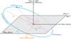Fig. 4 Diagram of the main orbital elements of a celestial body moving along its orbit (blue) intersecting the sky plane (grey) at the ascending node Ω0.

3 The PACOME algorithm

3.1 Reduced orbital elements

The orbits of PACOME were parametrized using a mix of the conventions described in Murray & Correia (2010) and Blunt et al. (2020). We used the semi-major axis (a), eccentricity (e), inclination (i), epoch of periapsis passage (τ), argument of periapsis (ω) and longitude of ascending node (Ω). To these six conventional orbital elements, we added a seventh and final parameter, namely, Kepler’s constant (K), to link the orbital period P to the semi-major axis while accounting for the total mass of the system without making any strict assumption on it nor on the distance of the object from the Earth.

The semi-major axis is expressed in milliarcseconds and all angular quantities (i, ω, Ω) in degrees. The longitude of ascending node Ω is oriented with respect to the true north direction and increases counterclockwise. The orientation of the inclination angle is such that i = 0° denotes a prograde orbit seen face-on whereas i = 90° denotes an edge-on orbit. The epoch of periapsis passage, τ, is expressed as a fraction of the orbital period with τ = t₀|P (mod 1), where t₀ is the traditional epoch of periapsis passage in years. Finally, Kepler’s constant K = a³|P² is expressed in milliarcseconds cubed per year squared. The derived period P is therefore expressed in years. The 2D reference frame coincides with the sky plane. Its origin is the central body (i.e., the host star), the x-axis is in the positive declination direction (ADec, north is up or true north) and the y-axis is in the negative right ascension direction (−ΔRA, east is left). Most of these orbital elements are represented in Fig. 4 and the chosen parameters are summarized in Table 2.

Orbits are usually degenerated as several combinations of orbital elements give the same projection on the 2D plane.

A typical example is the pairing (ω, Ω), which is perfectly equivalent to (ω + π, Ω + π). Orbits also become very degenerated for nearly face-on orbits (i ~ 0) and/or small eccentricities. While it is not possible to circumvent these degeneracies without additional constraints (e.g., system resonances), they do not affect the detection sensitivity of the proposed method (see Sects. 4.4.2 and 4.5.1).

To solve Kepler’s equation and project the 2D positions of a celestial body on the sky plane, we used Brent’s fzero method (Brent 1973). The equations for the Keplerian motion, the 2D projection, and the solver are described in more detail in Appendix B.

3.2 Optimization strategy

The cost function derived in Sect. 2 has several local maxima mostly due to the high dimensionality of the problem, the presence of noise in the data, and the speckles being similar to the PSF. Hence, finding the optimal solution cannot be performed by a local optimization method. To search for the global maximum of the criterion C(μ) of Eq. (10), we proceeded to sample C(μ) on a large 7D regularly spaced grid followed by a local optimization to refine the parameters.

3.2.1 Search space sampling

We used a regularly spaced 7D grid to exhaustively explore the parameter space but all orbital elements are not necessarily sampled at the same precision. This strategy has proven to be effective for the tests on the semi-synthetic data and on the HR 8799 system, detailed in Sects. 4.4 and 4.5. We stress that the 7D grid sampling should be thinner for far-out exoplanets with highly covered orbits.

Given the fairly small computation times required by the algorithm to explore a large number of orbits (≃20 min for 10 epochs, two spectral channels, and 10⁹ orbits on 12 CPUs), we did not find any urgent need for more complex methods though more advanced sampling and on-search grid refinement strategies will be explored in future works to decrease redundancies, while continuing to maintain an exhaustive approach, to derive the full orbital elements posterior distributions and ensure that the global maximum is found.

3.2.2 Local optimization refinement

After establishing the best on-grid orbit, a local refinement of the orbital elements is performed around the Nopt best solutions (typically the first 100 or 1000). To maximize the objective function, we use the VMLM-B optimization method (Thiébaut 2002), which is a memory-limited quasi-Newton method with bound constraints. It is quite similar to L-BFGS-B (Byrd et al. 1995) but has less overheads per iteration. Algorithms of this kind are particularly suitable for large-scale nonlinear problems compared to, for instance, constrained conjugate gradients. VMLM-B requires the objective function to optimize as well as its gradient. Given the reasonable number of iterations needed for the algorithm to converge, we set the tolerance thresholds for deciding of the convergence of the optimization so that the precision on the sought-for variables is close to the machine precision.

The required gradient of the multi-epoch criterion (Eq. (10)) is expressed as: $$\begin{array}{l}\frac{\partial 𝒷\left(\mu \right)}{\partial \mu }={\displaystyle \sum _{t,\ell }[2\frac{{\left[b_{t,\ell }\left({\theta }_t\left(\mu \right)\right)\right]}_{+}}{a_{t,\ell }\left({\theta }_t\left(\mu \right)\right)}\frac{\partial b_{t,\ell }\left({\theta }_t\left(\mu \right)\right)}{\partial \mu }}\hfill \\ -{\left(\frac{{\left[b_{t,\ell }\left({\theta }_t\left(\mu \right)\right)\right]}_{+}}{a_{t,\ell }\left({\theta }_t\left(\mu \right)\right)}\right)}^2\frac{\partial a_{t,\ell }\left({\theta }_t\left(\mu \right)\right)}{\partial \mu }],\hfill \end{array}$$(24)

and can be computed semi-analytically using the chain rule: $$\{\begin{array}{l}\frac{\partial b_{t,\ell }\left({\theta }_t\left(\mu \right)\right)}{\partial \mu }={\frac{\partial b_{t,\ell }\left(\theta \right)}{\partial \theta }|}_{\theta ={\theta }_t\left(\mu \right)}\cdot \frac{\partial {\theta }_t\left(\mu \right)}{\partial \mu },\hfill \\ \frac{\partial a_{t,\ell }\left({\theta }_t\left(\mu \right)\right)}{\partial \mu }={\frac{\partial a_{t,\ell }\left(\theta \right)}{\partial \theta }|}_{\theta ={\theta }_t\left(\mu \right)}\cdot \frac{\partial {\theta }_t\left(\mu \right)}{\partial \mu },\hfill \end{array}$$(25)

where the derivatives of the a_t,ℓ and b_t,ℓ terms with respect to the projected positions ∂a_t,ℓ/∂θ and ∂b_t,ℓ/∂θ are approximated using the derivatives of the interpolation function and where the derivatives ∂θ_t/∂μ of the projected positions with respect to the orbital elements are computed analytically. The details of the latter derivatives can be found in Appendix C.

Two other classical constrained optimization methods⁸ without derivatives were also tested: NEWUOA (Powell 2006) and BOBYQA (Powell 2009). However, VMLM-B showed better performance by refining the solution deeper, thus giving higher multi-epoch detection scores. Optimizing the solution with VMLM-B is also fast. It takes about 50 μs per evaluation of the cost function and its gradient with a cubic spline interpolator and a dataset consisting of T = 10 epochs, L = 2 spectral channels (see Sect. 3.4.1 for more details).

3.3 Inference of the uncertainties

We developed two methods to infer the local uncertainties associated with the optimal orbital solutions. The first is a perturbation method in which random realizations of Gaussian noise of the same order of magnitude as the variance of the signal are injected in the data and where the solution is re-optimized locally with the perturbed data to calculate confidence intervals on the orbital elements. The second method exploits the Cramér-Rao lower bounds (CRLBs) which are good estimates of the covariance of maximum likelihood estimators when the number of samples is large enough (Kendall et al. 1948).

3.3.1 Numerical method based on perturbations

For each epoch and spectral channel, we perturb the data by adding to the b_t,ℓ terms random noise realizations drawn in a centered Gaussian distribution with variance a_a,ℓ (see Sect. 2.1.3 for the derivation of the distribution of b_t,ℓ). For these new perturbed data, we re-optimize the criterion around the optimal solution, $\widehat{\mu }$, found for unperturbed data. We repeat this process a large number of times, N_p, to form a collection of optimal orbital parameters obtained with perturbed data, ${\left\{{\mu }_{\left(n\right)}\right\}}_{n=1:N_p}$. Then, we compute the lower and upper bounds of the confidence intervals (CI) associated to the obtained orbital elements distribution at a specified confidence level (e.g., 95%). As the samples are drawn independently, the number of draws N_p does not need to be very large (N_p ≃ 10⁵ is usually enough).

3.3.2 Analytical method based on CRLBs

From the expression of the multi-epoch log-likelihood of Eq. (8), we derived the Fisher information matrix of the orbital elements, μ, at epoch, t. It is expressed as a 7 × 7 matrix, I_t(μ), whose elements [I_t(μ)]_i,j are given by: $${\left[I_t\left(\mu \right)\right]}_{i,j}=\text{𝔼}\left\{\frac{\partial {\text{ℒ}}_t\left(\mu \right)}{\partial {\mu }_i}\frac{\partial {\text{ℒ}}_t\left(\mu \right)}{\partial {\mu }_j}\right\},$$(26)

where L_t(μ) is the log-likelihood at epoch, t. Distributing the derivative over the sum gives: $$\begin{array}{l}\frac{\partial {\text{ℒ}}_t\left(\mu \right)}{\partial {\mu }_i}={\displaystyle \sum _{\ell }(\frac{{\left[b_{t,\ell }\left({\theta }_t\left(\mu \right)\right)\right]}_{+}}{a_{t,\ell }\left({\theta }_t\left(\mu \right)\right)}\frac{\partial b_{t,\ell }\left({\theta }_t\left(\mu \right)\right)}{\partial {\mu }_i}}\hfill \\ -\frac{1}{2}{\left(\frac{{\left[b_{t,\ell }\left({\theta }_t\left(\mu \right)\right)\right]}_{+}}{a_{t,\ell }\left({\theta }_t\left(\mu \right)\right)}\right)}^2\frac{\partial a_{t,\ell }\left({\theta }_t\left(\mu \right)\right)}{\partial {\mu }_i}).\hfill \end{array}$$(27)

The derivatives of the b_t,ℓ and a_t,ℓ terms with respect to the orbital elements, μ, are computed via the chain rule mentioned in Sect. 3.2.2. By approximating the expectation of Eq. (26) to simply the product of derivatives, the Fisher information matrices of all independent epochs can be computed individually and gathered to encompass all multi-epoch information by simply summing over time: $$I\left(\mu \right)={\displaystyle \sum _t{I}_t\left(\mu \right)}.$$(28)

Thus, the multi-epoch covariance matrix of the orbital elements satisfies the CRLBs: $${\text{Cov}}^{\left(\text{CRLB}\right)}\left\{\mu \right\}\ge I{\left(\mu \right)}^{-1},$$(29)

where the square roots of the diagonal coefficients yield the lower bounds, ${\sigma }_{\mu }^{\left(\text{CRLB}\right)}$, of the standard deviations associated to the orbital elements. As epochs provide independent samples, the inequality of Eq. (29) tends to the equality as the number of epoch grows.

3.3.3 Comparison between both approaches

The analytical method based on CRLBs is faster than the numerical one but it can be sensitive to possible orbital elements degeneracies since it requires inverting an estimate of the Fisher’s information matrix. It also supposes that the errors are symmetric and Gaussian, however, they were shown not to be (Konopacky et al. 2016; Wertz et al. 2017; Wang et al. 2018). This approximation can only quantify the local error around the solution and fails totally to provides information on the global orbital elements distribution. The perturbation method explores more of the parameter space but still stays in the vicinity of the solution which is not enough. It is also biased (Ford 2005) as the multiple re-optimization processes always start from the optimal solution identified by PACOME.

Furthermore, both approaches account for the “local data fitting error” only, namely, the local uncertainty induced by the model given the data. In other words, the global distribution of the orbital elements on the full parameter space or additional sources of systematics errors related to the instrument itself, to calibration, and/or to pre-reduction issues are not accounted for. As both methods act locally on the orbital elements they do not deal with the degeneracies (i.e., multi-modal peaks in their distribution). This generally results in uncertainties different than those obtained with dedicated sampling algorithm such as MCMC (Ford 2005) or nested sampling (Skilling 2004) that will be explored in future studies. Even though the main focus of this work is the detection aspect, we use the perturbation method in the following (Sect. 4) to assess the local uncertainties of the orbital solutions with full awareness of the limits of our approach.

3.4 Implementation details

3.4.1 Interpolation strategy

To cope with the fact that the projected positions, θ_t(μ), do not necessarily coincide with the sampling positions of the maps, a_t,ℓ and b_t,ℓ, computed by PACO, we interpolate these maps to evaluate the criterion. The choice of the interpolation method is quite critical, as discussed hereafter.

To assess which interpolator is most suitable for our problem, we need a ground truth to quantify the goodness of the interpolation and, therefore, an assumption with respect to the shape of the signal of interest must be made. The off-axis PSF can be approximated by a 2D isotropic Gaussian. To identify the best possible interpolator, we generated S = 10⁴ 2D Gaussian PSFs, whose positions and amplitudes are known. The amplitudes of the synthetic PSFs are drawn uniformly between 5 and 30, and their full widths at half maximum were chosen to match the experimental conditions of the VLT/SPHERE-IRDIS and IFS instruments (wavelengths λ ∈ [0.95 μm, 2.32 μm] and a telescope diameter D = 8.2 m). Then, we interpolated each synthetic PSF in a M-pixel circular region of diameter d = 4σ with a sampling step six times smaller than the pixel size. We computed the absolute mean percentage of the recovered signal (AMPRS), as well as the root mean square error (RMSE), between the interpolated and ground truth amplitude values: $$\text{AMPRS}\left(\%\right)=100-\frac{100}{SM}{\displaystyle \sum _{s=1}^S{\displaystyle \sum _{m=1}^M\left|\frac{g_{s,m}^{\text{int}}-g_{s,m}^{\text{gt}}}{g_{s,m}^{\text{gt}}}\right|}},$$(30) $$\text{RMSE=}\sqrt{\frac{1}{SM}{\displaystyle \sum _{s=1}^S{\displaystyle \sum _{m=1}^M{\left(g_{s,m}^{\mathrm{int}}-g_{s,m}^{\text{gt}}\right)}^2}}},$$(31)

where g^int and g^gt are the interpolated and ground truth synthetic PSFs, respectively. Several interpolation functions⁹ were tested: nearest neighbor, bilinear, cubic B-spline, and four-neighbor Lanczos function, as well as two cubic cardinal splines: Mitchel & Netravali (ψ = −1/2, χ = 1/18) and Catmul & Rom (ψ = −1/2, χ = 0), where ψ and χ represent, respectively, the derivative and the value of the kernel function at position x = 1. We also performed a quick optimization with VMLM-B to find the best (in the RMSE sense) cubic cardinal spline (BCCS) coefficients for our problem. It yielded ψ ≈ −0.600 and χ ≈ −0.004.

The detailed results of the study are given in Table 3 and a graphical representation of the tested kernel functions are represented in Fig. 5. The BCCS and the Catmull & Rom spline give very similar results and are more efficient than the other comparative methods. We chose the BCCS interpolation for the rest of this work.

Fig. 5 Kernel functions of the tested interpolation methods.

3.4.2 Storing of the useful data

As the algorithm explores a very large number of orbits (10⁹ typically), the amount of data to be saved is substantial. Indeed, an orbit being encoded by seven parameters, storing all explored orbits as well as their multi-epoch scores would take about 500 Gb of space for double-precision floating-point numbers (64 bits × 8 × 10⁹), which is excessive.

Our parameter space is sampled regularly so the values of the orbital elements we explore are deterministic. We use this to our advantage and only store seven lists of variable sizes containing the discrete values of the orbital elements to explore, rather than storing all the orbital elements combinations. We assign a unique integer index to each orbital combination and use that instead. Doing so reduces the space taken to save the data by a factor of 4 (instead of 8), as we only need to store an integer and a double precision floating-point number.

In addition, most of the explored orbits do not fall on the projected position of the putative exoplanet and therefore contain no interesting information as they only combine noise. Hence, we only save the orbits whose multi-epoch cost function scores are greater than a given value that we typically set to the quan-tile function value associated to the confidence level of detection ρ = 0.01 (i.e., a 99% confidence level). Doing so reduces the number of saved orbits by a factor 100 which, combined with what is described above, brings the total space taken in memory by the PACOME products down to ≃1 Gb, whatever the number of epochs.

Finally, the indexes of the retained orbits and their multi-epoch scores are stored dynamically in memory-mapped files to avoid overcharging the random-access memory by loading a very large matrix.

3.4.3 Massive code parallelization and execution time

The entire algorithm is written in Julia (Bezanson et al. 2017), an open-source and strongly typed language designed for high performance programming. Coupling the intrinsic speed of Julia with massive code parallelization enables the algorithm to process very large numbers of orbits in a reasonable computation time. Even though PACOME can be run on a laptop, we used a local machine equipped with an Intel™ Xeon E5-2620 v3 CPU running at 2.40 GHz with 12 cores. The computational power achievable by this CPU is estimated at a maximum of 325 Gflops by the Intel™’s Math Kernel Library Benchmarks for Linux. Our implementation of PACOME does not use any GPUs.

Testing an orbit is done by selecting the orbit, computing its projected positions by solving Kepler’s equations, interpolating the a_t,ℓ and b_t,ℓ terms¹⁰, computing the cost function, assessing its value, and saving it in a memory-mapped file. This is done in approximately 12.6 × 10³ operations on average, which takes a typical execution time of 9 μs for T = 10 epochs and L = 2 spectral channels. Altogether, the PACOME algorithm takes about 20 min to assess 10⁹ orbits for the considered case (i.e., 12 cores, T = 10, and L = 2).

The a_t,ℓ and b_t,ℓ maps are pre-calculated via PACO’s reduction step upstream of PACOME and, hence, they do not need to be recomputed each time we run the algorithm. The execution time of this phase is variable but it usually takes several minutes up to several hours. For example, the ADI version of the PACO algorithm takes an hour to process (with ten threads on our machine) a rather large VLT/SPHERE-IRDIS hypercube of 500 frames, 1024 × 1024 pixels per frame, and two spectral channels with a patch radius of five pixels.

3.5 Summary of PACOME’s workflow

The PACOME algorithm starts by sampling the criterion of Eq. (10) on a 7D grid mapping the orbital elements search space. For that purpose, in a parallel loop, the subpixelic 2D projected positions θ_t are computed for each sample of the parameter space and for all epochs. The values of a_t,ℓ and b_t,ℓ terms at these positions are interpolated thus allowing the evaluation of the cost function. Then, the algorithm proceeds with the local optimization of the few best N_opt orbital solutions to find the one that maximizes the objective function. The score of the optimal solution is finally compared to the multi-epoch detection limit (i.e., at a confidence level of 1 − ρ) estimated numerically via the empirical statistical distribution of the criterion to decide on a potential detection (or otherwise). If a detection is claimed, the local uncertainties associated to the solution are computed via the perturbation method and/or with the CRLBs. A schematic diagram of the PACOME algorithm is represented in Fig. 6 and a pseudo-code is given in Algorithm 1.

Fig. 6 Schematic diagram of the PACOME algorithm.

4 Results

4.1 Datasets description

In this section, we evaluate the performance of the proposed algorithm on 23 datasets from both the InfraRed Dual Imaging Spectrograph (IRDIS; Dohlen et al. 2008a,b) and from the Integral Field Spectrograph (IFS; Claudi et al. 2008, 2010) of the VLT/SPHERE instrument (Beuzit et al. 2019). The observations were conducted with the A(S)DI technique using the pupil tracking mode of the instrument (see Sect. 1). The observations were scheduled so that the star was observed during meridian passage to take benefit, as best as possible, of the apparent rotation of the sought-for objects. All datasets correspond to observations of HR 8799 (HIP 114189), obtained under highly variable observing conditions between 2014 and 2021 (see Table 4 summarizing the main logs parameters).

HR 8799 is a A5V type star of the Pegasus constellation of mass $M_{★}={1.47}_{-0.17}^{+0.12}{M}_{\odot }$ (Sepulveda & Bowler 2022) and parallax of π = 24.462 ± 0.046 mas (Gaia Collaboration 2021). Until now, it has remained the sole star hosting four massive exoplanets discovered by direct imaging (Marois et al. 2008, 2010). These exoplanets orbit nearly coplanarly between 15 and 80 au, with a low eccentricity, and with a quasi-resonance of type 1:2:4:8. Three of them (HR 8799 c, d, and e) are within the IRDIS and IFS field of view, while the fourth one (HR 8799 b) lies only in the larger field of view of the IRDIS instrument. This system has been widely studied, in particular to characterize the orbits (see e.g., Maire et al. 2015; Zurlo et al. 2016; Wertz et al. 2017; Wang et al. 2018; Lacour et al. 2019), the atmospheres composition (see e.g., Currie et al. 2014; Ruffio et al. 2021; Wang et al. 2021), and the masses (see e.g., Marley et al. 2012; Brandt et al. 2021; Sepulveda & Bowler 2022) of the known exoplanets. The presence of a debris disk in the circumstellar environment and orbital stability studies showed that there is room for additional exoplanets, either interior or exterior of the known four exoplanets (Currie et al. 2014; Goz´dziewski & Migaszewski 2014; Wahhaj et al. 2021; Thompson et al. 2023). Despite the substantial efforts put into the analysis and combination of the available data, no candidate companion has been robustly identified. The current best results show a possible candidate of 4−7 M_Jup at 4−5 au, at a detection confidence of about 3σ in the L spectral band with KECK/NIRC2 (Thompson et al. 2023). However, this candidate companion is not detected with on-par or deeper observations from the VLT/SPHERE instrument at shorter wavelengths (Wahhaj et al. 2021). As a byproduct of the evaluation of the performance of the proposed algorithm, we also aim to put tight constrains (in terms of contrast) on an additional candidate companion in the HR 8799 system, as described in Sect. 4.5.

4.2 Pre-reduction

Raw observations were pre-processed with the pre-reduction and handling pipeline of the SPHERE consortium (Pavlov et al. 2008). Background, flat-field, bad pixels, registration, true north, wavelength, and astrometric calibrations are performed during this step. Additional custom steps implemented at the SPHERE Data Center (Delorme et al. 2017) were also applied to refine the wavelength calibration, reduce the crosstalk, and improve the identification of bad pixels. We also designed a new strategy to refine the conventional frame centering implemented in the SPHERE Data Center, as described in the following.

All the datasets of this work were acquired in pupil-tracking mode, namely, at a given epoch the field rotates around the star from a frame to another (see Sect. 1). In that context, having a precise knowledge of the rotation center is critical to maximizing the detection confidence and deriving accurate astro-photometric estimates of the putative sources in single-epoch datasets. In our case, the sought-for sources also orbit around the same rotation center defined by the star itself across epochs, so it is even more crucial to ensure that the rotation center is precisely known for all epochs. Unfortunately, it is not possible to use the central star to measure directly the rotation center because it is masked by the coronagraph. Conveniently, applying a waffle pattern to the deformable mirror while acquiring the observations creates (by diffraction) four replicas of the PSF so-called “satellite spots”, located around the rotation center at about 14 λ/D, where λ is the wavelength and D the diameter of the telescope (Langlois et al. 2012). The rotation center of all the frames of an A(S)DI sequence can thus be measured using the satellite spots, if their positions are precisely estimated. We re-addressed the previous numerical centering strategy that was used on the SPHERE Data Center by developing an algorithm that is faster and less sensitive to outliers (e.g., bad pixels and large stellar leakages). This leads to a better recentering procedure which improves the S/N of real sources (see Table D.1 for more details). Similarly to the work of Wang et al. (2014) for GEMINI/GPI, we implemented a new routine that fits 2D Gaussian functions to the satellite spots via a nonlinear least mean square constrained optimization method to estimate their subpixel locations. Based on these measurements, all the frames are shifted accordingly to match the measured rotation center to an arbitrary position satisfying the SPHERE Data Center and the PACO pipeline requirements. Our centering method has been delivered and integrated in the SPHERE Data Center (see Appendix D for more details and results).

After this pre-reduction step, raw observations were assembled in calibrated A(S)DI datasets. Each pre-reduced IRDIS observation is composed of L = 2 spectral channels that are processed both independently (i.e., akin to ADI sequences) and jointly (i.e., akin to ASDI sequences). Each pre-reduced IFS observation is composed of L = 39 spectral channels that are processed jointly. All pre-reduced datasets are first processed by the PACO pipeline (see Sect. 4.3), whose byproducts are then used by the proposed PACOME algorithm, see Sects. 4.4 and 4.5.

4.3 Reduction with PACO

The calibrated A(S)DI datasets described in Sect. 4.2 were processed with the PACO algorithm to produce, for each epoch, the a_t,ℓ and b_t,ℓ maps. These outputs serve as inputs of the PACOME algorithm (see Sect. 2.1). As discussed in Sect. 2.2, for the reduction of ASDI datasets, it is possible to enforce one or multiple spectral prior(s) γ є ℝ^TL to boost the S/N of detection of pointlike sources having a similar spectra¹¹. For ASDI processing of IRDIS observations, we chose seven spectral priors for the source corresponding to slopes of 0.25, 0.5, 0.75 and their opposites, namely, priors (1,1), (1,0.25), (0.25,1), (1,0.5), (0.5,1), (1,0.75), (0.75,1). For the IFS observations, we chose 23 spectral priors that are representative of the variety of potential exoplanets spectra, as described in Chomez et al. (2023), for the mode of selection of these spectral priors. The data are processed independently for each spectral prior (but jointly on the whole spectral range). We give equal importance to all the spectral priors used in this work. The only criterion to decide in favor of the presence of a planet is the combined multi-epoch score, whatever the underlying spectral prior, since no other information is known a priori.

4.4 Analysis of semi-synthetic data

4.4.1 Description of the datasets and of the injected orbits

To quantify the efficiency of PACOME, we tested it on a semisynthetic benchmark. We built ‘fake epochs’ by resorting to the injection of synthetic sources on a dataset of HR 8799 observed with IRDIS in 2016-11-18 (see Table 4 for the observations logs). By selecting individual frames from this reference dataset, we built nine fake epochs totalling 5.12 h of observation time and spanning over 59 yr. The ADI rotation angles of each fake epoch were chosen in the opposite direction of the original ones, so that signals from real exoplanets were not constructively co-added via the derotation and stacking of the individual frames. The total field of view rotation was set to ∆_par = 67.34° for each epoch.

We injected four sources, denoted as (1), (2), (3), and (4) in the following, on known orbits at the corresponding epochs via a PACO subroutine using the measured off-axis PSF of the reference cube. The injected fluxes of the sources were chosen such that their single-epoch S/N is lower than five on average. A summary of the fluxes, S/Ns, and separations of the injected sources at all epochs is given in Table 5. After the source injections, we reduced the nine semi-synthetic datasets with PACO.

4.4.2 Results of the search

To detect multiple sources, we adopted a simple greedy strategy: finding the brightest of the four planets with a first search, estimating its orbit, masking its footprint in PACO’s byproducts, b_t,ℓ, restarting the search for next brighter source, and so on. A summary of the explored search space for the four sought for sources is given in Table 6. We used the best cubic cardinal spline derived in Sect. 3.4.1 for the interpolation process. In total, N_orb ≈ 17 × 10¹⁰ orbits were tested, taking 44 h of CPU time on our local computer using 12 threads. For each search, the first N_opt = 10³ best on-grid orbits were optimized locally and the best of all was retained as the most plausible orbital candidates. The volume of the data is fixed and totals about 10⁶ pixels per epoch for IRDIS. Hence, the total number of possible multi-epoch combinations of all pixels in our data is 10^6×T×L = 10⁵⁴ compared to which the number of explored orbits is completely negligible. For this reason, we put the detection confidence in perspective with the number of explored orbits N_orb and set it at a high conservative value (ρ = 0.1/N_orb = 2.33 × 10⁻¹²) so that it is expected to experience one combined detection score above the multi-epoch detection threshold in the background 10% of the time with different PACOME runs. This threshold is arbitrary and it is left to the user to choose; in any case the empirical false alarm rate is controlled at the prescribed value. Given the T = 9 epochs and L = 2 spectral channels, the corrected empirical multi-epoch detection threshold at this confidence level is ${\widehat{Q}}_{18}^{\text{corr}}$(1 − 2.33 × 10⁻¹²) ≈ 48.3.

The orbital elements of the best source candidates are given in Table 7 and compared to the injected ones. The upper and lower confidence intervals for the orbital elements shown in this table were computed at a confidence level of 95% via the perturbation method with N_p = 10⁴. To evaluate the similarity between the 2D projected positions of the retrieved orbits $\hat{\mu }$ and the (ground truth) injected orbits µ^gt, we compute their root mean square distance (RMSD) as: $$\text{RMSD}\left(\widehat{\mu },{\mu }^{\text{gt}}\right)\text{=}\sqrt{\frac{1}{T}{\displaystyle \sum _{t=1}^T{\Vert {\theta }_t\left(\widehat{\mu }\right)-{\theta }_t\left({\mu }^{\text{gt}}\right)\Vert }^2}}.$$(32)

The RMSD formulation is a convenient tool that can be used to assess how good the algorithm is when it comes to fit the original injected orbit. The projections of the optimal retrieved orbits of Table 7 along with the best other 10³ optimized orbits are shown in Fig. 7. In addition, we plot the cost function maps of the criterion centered on each of these optimal solutions in regions of interest (ROIs) of 60 pixels wide sampled with four nodes per pixel in Fig. 8. The color maps are specifically centered on the corrected multi-epoch detection threshold ${\widehat{Q}}_{18}^{\text{corr}}$(1 − p) such that any signal above the limit (in dark red) can be interpreted as statistically significant regarding the set detection confidence p = 2.33 × 10⁻¹².

The retrieved orbits agree very well with the ground truth (Table 7) except for the argument of periapsis, ω, of source (4), which is significantly different and is not captured by our uncertainties (underestimated because they were performed locally; see Sect. 3.3.3). However, the projected solution found by PACOME is still very close to the ground truth as it gives almost the same positions on the detector at thegiven epochs (RMSD = 0.2 pixels). Remarkably, for each of the four sources, the RMSD of the projected positions is always lower than 3/4 of a pixel, which indicates the closeness between tlie solutions retrieved by PACOME and the projections of the ground truth orbits. We also notiee in Fig. 7 a very different variety of orbits among the 10³ best optimized orbits for sources (2), (3), and (4). Most of the atypical orbits would correspond to putative sources wirth a murti-epoch S/N lower than 3.3. In practice, they correspond to the recombination of reeidual noise, which is statistically expected in this low, S/N regime.

Apart from the four injected sources effectively retrieved with PACOME, no other signals were found above the chosen multi-epoch detection threshold, as statistically expected by our statistical model. To validate the reliability of our detection metric, we masked the four retrieved sources and re-explored the orbital parameters space on the masked data to build the effective distribution of the multi-epoch S/N in the absence of source. In total, 2 × 10⁸ orbits were drawn uniformly in the parameter space, with Table 6 displaying the allowed ranges. In Fig. 9, the multi-epoch S/N detection thresholds associated to this distribution (i.o., the ground truth) are compared to the actually used detection thresholds estimated with the power” law of Eq. (15). The absolute relative error between the two estimations is 3.2% on average and always below 5%, over the whole range ρ є [10⁻⁶,10⁻¹], while the corresponding RMSE is 0.14 in terms of the S/N. Given these errors are relatively low, this indicates that the detection metric is well controlled even though the threshold estimated via the power law (used in this paper) is systematically (mildly) over-estimated, which is conservative. As a result, we experience slightly fewer false alarms than theoretically expected for a given threshold.

As expected (and more precisely discussed in Sect. 3.3.3), the uncertainties on the orbital elements are estimated locally. As a consequence, they are optimistic and smaller than what would be obtained using more classical orbit-fitting methods in the literature that effectively explore the full parameter space (Ford 2005).

The criterion values for the optimal orbital solutions found by PACOME (Table 7) are all significantly higher than the empirical multi-epoch detection limit at ρ = 2.33 × 10⁻¹² (by a factor of at least 2), while the vast majority of the point-like sources remain undetected in each individual epoch (S/N_t,ℓ < 5 by applying only the PACO algorithm; see Table 5 and Appendix E for a local view of S/N_t,ℓ maps). In particular, the mean mono-epoch S/N_t,ℓ of the optimal solutions (averaged over the T = 9 epochs and L = 2 spectral channels) are 4.0, 2.2, 2.4, 2.3 and their multi-epoch S/N are 18.5, 9.9, 10.5, 10.2, from source (1) to (4), respectively. This means that switching from mono-epoch to multi-epoch yields a mean S/N gain of about 4.5, which behaves (as theoretically expected) as the square root of the number of degrees of freedom ( $(\sqrt{T\times L}=\sqrt{18}\approx 4.2)$. This illustrates a key property of PACOME: it is indeed able to combine optimally the source signals of single-epoch datasets. For completeness, we notice in practice that the values of the criterion associated with the optimal orbits found by PACOME are very slightly larger than the theoretically expected ones for the injected orbits. This is due to the presence of noise in the data. Indeed, the algorithm maximizes the signal around the optimal positions found and, thus, it captures the random noise realizations that co-add positively with the signal. As a result, the solutions have systematically slightly stronger criterion values than the injections and the RMSD between them are not perfectly 0.

Finally, Fig. 8 shows the cost function maps around the optimal solution estimated by PACOME. All signals in the field that are not at the source positions combine weakly (from blue to white colors, below the set confidence level at ρ = 2.33 × 10⁻¹²). However, because the sought-for signals are very faint and that the hypothesis of independent spectral channels is not perfectly verified, we sometimes recombine noise or speckles in the background. We show in Sect. 4.5.2 that explicitly accounting for the spectral correlations reduces this side effect. In any case, the optimal solution found by PACOME still matches its best with the ground truth. It is worth noticing that the method is very efficient at recovering injected sources that would have remained undetected otherwise. In particular, those are (2), (3), and (4), whose S/N values are below 5 for all individual epochs.

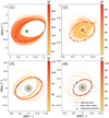Fig. 7 Optimal orbits Sound for each of the tour injected sources along with the best 103 other re-optimized orbits. The red thick line shows the retained optimal orbit, see Table 7. The blue dots art the projected positions of the signal along the optimal orbit ot all epochs and rhe grey circular area represents the largest coronagraphic masi

4.5 Analysis of HR 8799 archival data

4.5.1 Retrieving the four known exoplanets b, c, d, and e

In this section, we demonstrate the efficiency of the method on real A(S)DI data of HR 8799 acquired with SPHERE-IRDIS. The four exoplanets have already been detected in each of the individual epochs and spectral channels, hence, the following results show the ability of the algorithm to find matching orbits, rather than to (re)detect the sources.

The orbital elements search space is summarized in Table 8. It was deliberately chosen to cover a wide field of view encompassing all four known exoplanets. The cost function was evaluated for 20.5 × 10⁹ orbits in total. With this setting, the computation took about 22 h on 12 cores.

Considering the distance of the four exoplanets to the central star, the temporal coverage of the data allows to cover only a small portion of their orbit. The respective orbits of the four exoplanets are thus very poorly constrained. In order to disentangle the orbits from each other, we computed their RMSD to the center of the image (thus its pixelic distance to the star), with θ₀ as the position of the center of the images: $$\text{RMSD}\left(\widehat{\mu }\right)\text{=}\sqrt{\frac{1}{T}{\displaystyle \sum _{t=1}^T\Vert {\theta }_t\left(\widehat{\mu }\right)-{\theta }_0\Vert }}.$$(33)

This metric is a re-definition of the distance given in Eq. (32), by replacing the (unknown) ground truth θ_t(µ^gt) with θ₀. We show in Fig. 10 the distribution of the explored orbits with respect to their cost function and RMSD distance to the star. We distinguish four very sharp peaks at 140, 77, 56 and 32 pixels from the center. These peaks correspond to the orbits whose 2D projections at all times fall on (or very close to) the effective positions of the exoplanets HR 8799 b, c, d, and e (from right to left, respectively).

Concerning the orbits of the four planets, Wang et al. (2018) and Goździewski & Migaszewski (2020) found that a coplanar configuration near the 1:2:4:8 resonance produces orders of magnitude more stable orbits than any other scenario (i.e., orbiting with the same inclination i and longitude of the ascending node Ω). This can be used to constrain the optimization process of each orbit. We considered ω, Ω, and K to be fixed for each of the four exoplanets (i.e., coplanarity and orbiting the same central star) and therefore we carried out a joint search in the four peaks for the combination of four orbits that satisfy strict coplanarity (i.e., same i and Ω), common host star (i.e., same K), and near orbital resonance (i.e., 1:2:4:8 + 0.25). A total of 37 orbit quadruplets were found and are shown in Fig. 11. For each, the quadratic sum of the individual cost scores was optimized under the constrains described above and the best one was retained (highlighted in red).

The retained optimal orbital elements are detailed in Table 9. The semi-major axis, a, the eccentricity, e, the epoch of periapsis passage, t₀, the Kepler constant, K, and the period, P, that we derived are consistent with the literature values (Konopacky et al. 2016; Wertz et al. 2017; Wang et al. 2018; Lacour et al. 2019). However, the inclination, i, the argument of periapsis, ω, and the longitude of the ascending node, Ω, do not always match. We observed differences in Ω and ω, as our uncertainty quantification method does not explore all parameter space and fails to capture the highly degenerate cases of quasi-circular (e ≃ 0) and slightly inclined (i ≃ 0°) orbits (and even more so in cases of poor temporal coverage). In addition, the retained inclination, i, seems to be slightly underestimated by our method (i ≃ 8.9° compared to ≃20–25° in the literature). This tends to increase the total number of possible degeneracies on Ω, ω, and т and reinforces the difference we observe. On the other hand, 17 orbital combinations out of the 37 re-optimized ones (≃46%) have inclinations between 20 and 30 degrees which means that the commonly accepted range of values for the inclination of the four HR 8799 exoplanets is found by the algorithm and is very plausible. The projections of the optimal orbits of the four exoplanets are shown in red in Fig. 12, whereas the orange trajectories represent the first 10³ best other solutions whose RMSD are less than 1 pixel away from the optimal retained solutions (see Eq. (33)). Again, the poor temporal coverage of the data is clearly noticeable and shows that a large number of rather different orbits actually fall on the projected positions of the detected exoplanets.

The associated multi-epoch detection scores and S/N are extremely high (e.g., HR 8799 e is detected at S/N = 231), which again highlights the capability of the proposed algorithm to recombine efficiently faint signals from point-like sources, thus increasing the accuracy of the spectral characterisation of exoplanets. However, the gain in S/N does not scale as the square root of the number of epochs (see Table 9). This behavior was expected as the quality of the data is very heterogeneous across the 23 epochs, resulting in several epochs weighting much more than the others in the multi-epoch combination. Yet, even the worst epochs bring valuable information and constrain the solution (e.g., by eliminating some possible orbits). Finally, the multi-epoch cost function maps of the retained solutions are displayed in Fig. 13. As for the numerical experiments of Sect. 4.4, all signals in the field that are not at the exoplanet locations combine weakly (from blue to white colors, below the set confidence level at ρ = 4.9 × 10⁻¹²).

Fig. 8 Cost function maps around the optimal solution estimated by PACOME for each injected source in a ROI of 50 pixels wide sampled with four nodes per pixel. The value of the empirical multi-epoch detection threshold ${\widehat{Q}}_{46}^{\text{corr}}$(1 − 2.33 × 10−12) ≈ 48.3 is highlighted in green in the color bar.

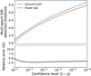Fig. 9 Comparison between the multi-epoch detection threshold estimated on the distribution out of the data in the absence of source and the one approximated by the power law of Eq. (15).

Fig. 10 Distribution of the explored orbits with respect to their cost function scores and their RMSD to the center of the images. Each blue dot represents an orbit.

Fig. 11 All 37 optimized orbit combinations of the search on the HR 8799 system satisfying the constraints of coplanarity, near resonance, and identical stellar mass. The best combination is shown in red whereas the 36 others are plotted in grey. Blue dots represent the 2D projected positions of each source at all epochs.

Fig. 12 Optimal orbits found for each of the four known exoplanets HR 8799 b, c, d, and e along with the best 103 other on-grid orbits (in orange to red colors), whose RMSD is less than 1 pixel away from the optimal solution. The red thick line shows the retained optimal orbit (see Table 9). The blue dots are the projected positions of the signal along the optimal orbit at all epochs and the grey circular area represents the coronagraphic mask.

Fig. 13 Cost function maps around the optimal solution estimated by PACOME for the four known exoplanets of the HR 8799 system in a ROI of 60 pixels sampled with four nodes per pixel. The value of the corrected empirical multi-epoch detection threshold ${\widehat{Q}}_{46}^{\text{corr}}$(1 − 4.9 × 10−12) ≈ 150.8 is highlighted in green in the color bar.

Fig. 14 Cost function maps around the optimal solution estimated by PACOME for three of the four known exoplanets of the HR 8799 system considering spectrally correlated (left) and spectrally whitened (right) observations from the SPHERE-IFS. A flat spectrum γ has been used as spectral prior for the spectral combination by PACO. The region of interest is 100 pixels wide and sampled with four nodes per pixel. The value of the corrected empirical multi-epoch detection threshold ${\widehat{Q}}_{15}^{\text{corr}}$(1 − 1.8 × 10−10) ≈ 69.5 is highlighted in green in the color bar.

4.5.2 Benefits of accounting for spectral correlations

At the end of Sect. 4.4.2, we discuss the fact that PACOME still managed to find the ground truth even though the hypothesis of independent spectral channels was not perfectly verified. The spectral correlations were in fact negligible because SPHERE-IRDIS data only feature L = 2 spectral channels. On the other hand, SPHERE-IFS data have L = 39 different spectral channels; thus, the spectral correlations are much stronger and it becomes essential to take them into account before carrying out the multi-epoch combination.

To illustrate the importance of whitening the data spectrally, we show in Fig. 14 the 2D maps of the multi-epoch criterion centered on the positions of HR 8799 с, d, and e, described in the section above for IFS data combined with and without the spectral correlation corrections. When we are not taking the spectral correlations into account, a larger number of structured patterns (noise and/or speckles) are combined positively and increase the background signal, thereby going above the prescribed detection level. Explicitly accounting for the spectral correlations reduces this side effect greatly so that solely the real known sources lie above the set detection limit.

We quantified the importance of accounting for the spectral correlations of the data by counting the number of false alarms (considering circular patches of the size of the FWMH) in the criterion map of the multi-epoch SPHERE-IFS dataset of HR 8799. This study was carried by accounting for the spectral correlations and by ignoring them for different confidence levels and the results are plotted in Fig. 15. The spectral whitening effect is undeniably efficient in reducing the number of false alarms (a factor of 600 at the ρ = 10⁻⁵ confidence level and a factor of 1800 at ρ = 10⁻⁶). At ρ ≈ 6 × 10⁻⁸ and below, false alarms are no longer found in the spectrally whitened data whereas the opposite case still rates very high number of false alarms (>2800).

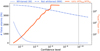Fig. 15 Number of false alarms (FA) for both the spectrally whitened (W) and not-spectrally whitened (NW) multi-epoch SPHERE-IFS datasets of HR 8799. The ratio between the two is shown in red. The number of multi-epoch false alarms was counted considering circular patches of the size of the FWMH. The grey vertical line corresponds to the chosen confidence of detection.

4.5.3 Search for a fifth planet

Several dynamical studies suggested that a fifth companion could orbit HR 8799 either in the outer region of the system (beyond HR 8799 b) between 90 and 110 au (Zurlo et al. 2022) or in the innermost part (before HR 8799 e) between 7.5 and 9.7 au (Wahhaj et al. 2021). We probed these two regions with PACOME to seek a potential candidate or to put constraints on its potential presence.

Derivation of the multi-epoch contrast. Building contrast curves is not straightforward when combining multi-epoch direct imaging observations and should be considered with care. With mono-epoch datasets, the achievable 5σ contrast is classically quantified at a given angular separation; whereas in a multi-epoch framework the combined contrast is computed for a given orbit where the angular separation of the source may vary along its trajectory. Hence, to compare the multi-epoch contrast to the more classical mono-epochs ones, we have to restrain the hypothesis and consider only face-on (i = 0) circular (e = 0) orbits. Given our model, we also need to assume that the flux of the source is constant over the epochs, which is consistent with face-on and circular orbits. These assumptions are restrictive but still more or less hold for the case of HR 8799 (Wang et al. 2018; Goździewski & Migaszewski 2020).

Under these assumptions, the constant source flux equals: $$\forall t\in \left[1,T\right],{\widehat{\alpha }}_{t,\ell }\left(\mu \right)={\widehat{\alpha }}_{\ell }\left(\mu \right)=\frac{{\sum }_t{b}_{t,\ell }\left({\theta }_t\left(\mu \right)\right)}{{\sum }_t{a}_{t,\ell }\left({\theta }_t\left(\mu \right)\right)},$$(34)

and, hence, the associated multi-epoch contrast is given by: $${\widehat{\sigma }}_{\ell }\left(\mu \right)=\sqrt{\text{Var}\left\{{\widehat{\alpha }}_{\ell }\left(\mu \right)\right\}}=1/\sqrt{{\sum }_t{a}_{t,\ell }\left({\theta }_t\left(\mu \right)\right)}.$$(35)

As stated in Sect. 2.1.3, our direct model implicitly accounts for the attenuation of off-axis PSFs near the coronagraphic mask (encoded in the a_tℓ and b_tℓ terms) therefore no multiplicative scaling is necessary.

The computed mono-epoch and multi-epoch 5σ contrasts curves are given in Fig. 16 and compared to Wahhaj et al. (2021) who presented the deepest contrast limits to date constraining the presence of a potential additional inner planet. Their datasets consist of 4.5 h of observations in K1–K2 band with IRDIS and Y-H band with IFS. Our work combines more datasets (23 for IRDIS, 15 for IFS) and achieves an even deeper contrast at all separations.

Outer part. The search in the outer part was carried out in ASDI mode with the SPHERE-IRDIS data because the region is not covered by the field of the IFS. We used a combination of (i) the 13 spectrally whitened dual-band datasets reduced with a flat prior spectrum and (ii) the first spectral channel of the 10 remaining broad-band datasets (as both channels carry more of less the same information).

We explored a total of N_orb ≃ 43 × 10⁹ orbits covering the same parameter space (as described in Sect. 4.5.1) for Kepler’s constant K, semi-major axis values from 2205 to 2696 mas, eccentricities from 0 to 0.5, and all allowed ranges for the remaining orbital elements.

For the same reason described in Sect. 4.4.2 and given the number of explored orbits, we set the desired confidence level to ρ = 0.1/N_orb = 2.3 × 10⁻¹² with ${\widehat{Q}}_{23}^{\text{corr}}$(1 − ρ) ≈ 76.2. No signals were found above this threshold. At these separations, the multi-epoch contrast limit is $\widehat{\sigma }\left(\mu \right)=1.2\times {10}^{-8}$ (see Fig. 16). The family of orbits with the highest multi-epoch criteria was found at projected positions 2582 mas away from the star and its best optimized orbit scored a 𝒷 = 69.9, corresponding to a confidence level of detection ρ = 8.7 × 10⁻¹¹, which is expected to happen around four times given the number of explored orbits. This family of plausible orbits is mostly driven by epochs 2017-10-12 and 2017-10-13, which always give the same projected positions on the detector. Alone, they explain 41% of the cost function score. This could be explained by an instrumental artefact, static on the scale of a day. The assumption of independent epochs on which the algorithm is based is violated in this case and there is no simple way to counter these systematics. In addition, the best optimized orbit (below the detection threshold) is not at all in the same orbital plane as HR 8799 b, c, d, and e (i = 77.6°) and its high eccentricity (e = 0.5) makes it cross the orbits of the other planets of the system which, for stability concerns, weakens considerably the possibility of a false negative candidate.

Inner part. For the search in the inner part of the system, we used the 15 SPHERE-IFS data described in Table 4. The three known visible sources were masked. Similarly, a part of the region under the coronagraph (80%) was masked since the transmission is very low in this area. In total, N_orb = 5.44 × 10⁸ orbits were explored, probing the semi-major axis parameter space from 122 to 246 mas, eccentricities from 0 to 0.5 and the same as the outer search for the remaining orbital elements. The confidence level was set to ρ = 0.1/N_orb = 1.8 × 10⁻¹⁰ yielding a detection threshold of ${\widehat{Q}}_{15}^{\text{corr}}$(1 − ρ) ≈ 69.5. The multi-epoch contrast limit is $\widehat{\sigma }\left(\mu \right)$ for these separations (see Fig. 16).

Among the 23 spectral priors used for the IFS data reduction step, only 4 (respectively one flat, two bi-modal, and one tri-modal priors) show optimized orbits with multi-epoch scores 2 to 11% greater than the prescribed detection threshold. None of the best orbits found for each spectral prior are alike or have the same projected positions on the detector. A closer inspection reveals that for each of the four identified priors the multi-epoch score is only driven by a handful of epochs (two or three). Indeed, the best three epochs of each prior contribute respectively to 64%, 76%, 72%, and 53% of their associated multi-epoch criterion.

We analyze these results as follows. First, having several different spectral priors giving a multi-epoch score above the limit is expected. As the same data is used for all priors, they can not be considered independent, so that a detection with one prior could yield an other detection for a different spectral prior. Second, the region that is explored here is very close to the central star, which is typically where slight residual non-stationarities can occur and where the assumed model for the off-axis PSF is not fulfilled (due to high nonlinearities induced by the corona-graph). Thus, the hypothesis on which our model is based (i.e., spatial correlations fully captured by a multi-variate Gaussian, spatially invariant off-axis PSF) are not perfectly verified in this regime and even more so in our multi-epoch case where the nuisance propagates and amplifies when combined temporally. To tackle this problem and reduce these effects, it would be necessary to model the correlations at larger scales and to consider a variable off-axis PSF in the field (e.g., via a grid of physical models) but this is not treated in this paper and is left for future works. Third, the fact that only a fifth of the epochs contribute to more than half of the criterion reflects an important need to explicitly take into account the consistency of the individual temporal S/N. This will avoid giving too much credit to (still rare) quite high detection peaks in some isolated individual epochs. Further works will be led to take this aspect into consideration and to quantify its benefits with respect to the current algorithm.

Finally, we ran the same search, but this time with the SPHERE-IRDIS data. No signals were found above the detection threshold considering the 13 dual-band datasets only. Taking the broad-band ones into account led to a few multi-epoch detections but all were ruled out because only driven by a mono-epoch false alarm detection near the coronagraphic mask in the 2017-10-12 epoch. Again, PACO suffers from the above-mentioned phenomenon close to the coronagraph, so if there is a false detection in a mono-epoch PACO map, it will inevitably yield a false alarm in the multi-epoch case.

Fig. 16 Mono and multi-epoch 5σ contrast curves of the IRDIS (left) and IFS (right) datasets of HR 8799 in ASDI mode with flat spectral priors. The multi-epoch contrast is computed as a function of the separation assuming face-on circular orbits and a source flux constant over the epochs. The 5σ contrasts found in Wahhaj et al. (2021) were extracted and overplotted for comparison.

5 Conclusion

In this work, we propose PACOME, a new algorithm dedicated to the combination of multi-epoch angular and spectral differential observations in high contrast obtained using the pupil tracking mode. As with other algorithms of this category, it integrates a massive search over the possible Keplerian orbits spanned by the putative sources, as well as a novel maximum likelihood multi-epoch detection score. Concerning the exploration of the plausible orbits, we designed an efficient two-steps strategy combining a coarse search on a grid with a local refinement of the best orbits found on this grid. The proposed multi-epoch metric directly derives from an end-to-end statistical framework, which explicitly accounts for the non-stationarity and the multiple and complex correlations of the data (spatial and/or spectral and/or temporal). It conveniently makes use of the byproducts of applying PACO, a powerful post-processing algorithm of mono-epoch observations at high contrast. Our new metric offers a reliable multi-epoch detection criterion, which is interpretable both in terms of probabilities of detection and false alarms. Jointly, PACOME also produces a few plausible estimates of the detected sources orbital elements and assesses their uncertainties locally. From an implementation point of view, we also integrated a new centering routine of the individual frames in our pipeline to increase the accuracy of the host star centering and, consequently, to improve the detection confidence of real sources.

We showed from realistic numerical experiments that the proposed approach is able to detect faint point-like sources that remain undetectable by advanced post-processing of each individual epoch. We obtained a gain in terms of detection sensitivity very close to the square root of the number of epochs, which corresponds to an optimal combination of the available information. As a case-study example, we applied PACOME on 23 VLT/SPHERE observations of the HR 8799 star. From these observations, we were able to re-detect the four known exoplanets at unprecedented levels of confidence (from S/N = 231 for planet e to 530 for planet b). In addition, we obtained the deepest level of contrast especially at close angular separation (3.0 × 10⁻⁶ for IFS and 1.7 × 10⁻⁶ for IRDIS at 0.125″) by combining all the available VLT/SPHERE datasets for this system.

We believe that the high detection sensitivity of PACOME opens the door to a massive re-exploration of the archived high contrast observations, possibly from different instruments. As an illustration for the VLT/SPHERE instrument, this analysis would at least concern HD 95086, HIP 65426, 51 Eridani, GJ 504, and Proxima Centauri that have been observed multiple times representing at the very least 80 observations (IRDIS and IFS combined) totalling a total exposure time of about 90 h. Such dedicated PACOME’s study will be conducted in a future paper. Besides, in the context of the forthcoming 30-meter class telescopes, our approach would be key to probe the habitable zone of the nearby stars and reach the deepest possible contrast limits. This will require long exposure times of several tens of hours that will only be achieved by combining several observations conducted days, weeks, or months apart. At these timescales and separations, the orbital motion of exoplanets will no longer be negligible and a proper orbital modelling will be crucial to combine multi-epoch observations without drastically degrading the detection confidence and the achievable contrast. PACOME’s outputs could also allow for the simulation of the experienced combined S/N for a given set of parameters (e.g., orbits, observing conditions, spectral band, parallactic rotation, exposure time, etc.). This will be essential for optimizing the use of the observational facilities by predicting the best observational times and parameters to maximize the scientific return. Concerning methodological developments, we are currently working on the refinement of the proposed algorithm by (i) further improving its robustness against the highly variable observation quality, (ii) improving the statistical model of the nuisance to account for correlations at longer spatial scale, and (iii) accounting for the variations of the exoplanetary signature across epochs and during the sequence of observations itself. As a longer term goal and in the context of the next generation of instruments designed to scrutinize the vicinity of nearby stars, we aim to develop a multi-epoch combination algorithm accounting jointly for the presence of point-like sources and of spatially resolved objects such as circumstellar disks.

Acknowledgements

We thank Frédéric Vachier (IMCCE, Observatoire de Paris, France) for fruitful discussions. We Thank Antoine Chomez and Philippe Delorme for their help with the data preprocessing. This work has made use of the SPHERE Data Center, jointly operated by OSUG/IPAG (Grenoble, France), PYTHEAS/LAM/CESAM (Marseille, France), OCA/Lagrange (Nice, France), Observatoire de Paris/LESIA (Paris, France), and Observatoire de Lyon/CRAL (Lyon, France). This work has been supported by the French National Programs (PNP and PNPS), and by the Action Spécifique Haute Résolution Angulaire (ASHRA) of CNRS/INSU co-funded by CNES. This work used ESO archive data for HR8799 from various observing programms with ESO-IDs listed in Table 4.

Appendix A Deriving an optimal multi-epoch S/N

A.1 Matched filter formalism

Here, we consider a general case where some data, d ∊ ℝⁿ, are measured under reproducible conditions parameterized by ϕ ∊ ℝ^p. These parameters account for the experimental conditions, the object of interest, and so on. It is always possible to express the following: $$d=m+z,$$(A.1)

with m = 𝔼{d | ϕ} as the expectation of the measurements under given conditions, ϕ, and z ∊ ℝⁿ representing a nuisance term accounting for the measurement noise. It directly follows that 𝔼{z | ϕ} = 0; in other words, the noise term, z, is centered knowing conditions, ϕ.

We then consider a measurable quantity, say, η ∊ ℝ, which linearly depends on the data: $$\eta =q^{\top }d,$$(A.2)

with q ∊ ℝⁿ the vector of coefficients of the linear combination, which may depend on ϕ. Our goal is to find the coefficients q that yield η with the highest possible S/N given the data. The expectation and variance of η under given conditions, ϕ, are: $$\{\begin{array}{ll}𝔼\left\{\eta |\varphi \right\}\hfill & =q^{\top }m,\hfill \\ \text{Var}\left\{\eta |\varphi \right\}\hfill & =q^{\top }Sq,\hfill \end{array}$$(A.3)

with S = 𝔼{z z^⊤ | ϕ} = Cov{d | ϕ} the covariance of the nuisance term z under given conditions ϕ, which is also the covariance of the data d under the same conditions. The S/N of η under the given observing conditions is then: $$𝒮/𝒩\left(\eta |\varphi \right)=\frac{𝔼\left\{\eta |\varphi \right\}}{\sqrt{\text{Var}\left\{\eta |\varphi \right\}}}=\frac{q^{\top }m}{\sqrt{q^{\top }Sq}}.$$(A.4)

Noting that for any γ > 0, the S/N of η and γ η are equal, it follows that the linear quantity of highest S/N is determined up to a positive factor. We can therefore maximize the S/N of η under the constraint that, say, its expectation, 𝔼{η | ϕ}, has a given value. Under that constraint, maximizing the S/N amounts to minimize the denominator in the right hand side of Eq. (A.4), that is q^⊤ S q the variance of η. The Lagrangian of this constrained problem is expressed as: $$ℒ=\frac{1}{2}{q}^{\top }Sq-\xi q^{\top }m,$$(A.5)

with ξ ∊ ℝ the Lagrangian multiplier associated to the constraint that 𝔼{η | ϕ} has a given value (the 1/2 factor is for convenience). Provided that the covariance S is invertible, the optimal solution of the Lagrangian is given by: $$q=\xi S^{-1}m,$$(A.6)

which is known as the “matched filter” (Kay 1998a,b). If q is the matched filter, the best possible S/N of η is then obtained for any ξ ≠ 0 and is equal to: $$\underset{q}{\max }𝒮/𝒩\left(\eta |\varphi \right)=\sqrt{m^{\top }{S}^{-1}m},$$(A.7)

which, as expected, does not depend on the multiplier ξ ≠ 0. Also, as expected, the optimal filter, q, and thus the optimal quantity, η, are defined up to a factor of ξ.

A.2 Application to multi-epoch detection

To apply the matched filter formalism described above to the direct model of A(S)DI observations given in Eq. (1), we consider the residual data: $$d_{t,\ell ,k}=r_{t,\ell ,k}-{\overline{f}}_{t,\ell },$$(A.8)

where d_t,ℓ,k is assumed Gaussian distributed with expectation α_t,ℓ h_t,ℓ(θ_t(µ)) and variance ${\sigma }_{t,\ell ,k}^2{\text{C}}_t$. Assuming that residual data from different epochs, frames, and/or spectral channels are mutually independent, the quantity of maximal S/N is: $$\begin{array}{l}\eta =\xi {\displaystyle \sum _{t,\ell }{\alpha }_{t,\ell }{\displaystyle \sum _k{h}_{t,\ell }{\left({\theta }_t\left(\mu \right)\right)}^{\top }{W}_{t,\ell ,k}{d}_{t,\ell ,k}}}\hfill \\ =\xi {\displaystyle \sum _{t,\ell }{\alpha }_{t,\ell }{b}_{t,\ell }\left({\theta }_t\left(\mu \right)\right)}.\hfill \end{array}$$(A.9)

Given the data and accounting for the assumed independencies, the best achievable S/N is obtained from Eq. (A.7): $$\begin{array}{l}\max 𝒮/𝒩\left(\mu \right)=\sqrt{{\displaystyle \sum _{t,\ell ,k}{\alpha }_{t,\ell }^2{h}_{t,\ell }{\left({\theta }_t\left(\mu \right)\right)}^{\top }{W}_{t,\ell ,k}{h}_{t,\ell }\left({\theta }_t\left(\mu \right)\right)}}\hfill \\ =\sqrt{{\displaystyle \sum _{t,\ell }{\alpha }_{t,\ell }^2{a}_{t,\ell }\left({\theta }_t\left(\mu \right)\right)}}.\hfill \end{array}$$(A.10)

When considering the maximum likelihood estimator of α_t,ℓ, this theoretical value can be approximated by the following (biased) estimator: $$𝒮/𝒩\left(\mu \right)=\sqrt{{\displaystyle \sum _{t,\ell }\frac{{\left({\left[b_{t,\ell }\left({\theta }_t\left(\mu \right)\right)\right]}_{+}\right)}^2}{a_{t,\ell }\left({\theta }_t\left(\mu \right)\right)}}}=\sqrt{𝒷\left(\mu \right)}.$$(A.11)

Appendix B Keplerian motion solver

The 2D position of a celestial body of orbital elements, µ = [a, e, i, τ, ω, Ω, K]^⊤, projected on the sky plane at the epoch of observation t is expressed as: $${\theta }_t\left(\mu \right)=r_t\left(\begin{array}{c}\cos \text{\hspace{0.17em}Ω\hspace{0.17em}cos}\left(\omega +v_t\right)-\sin \text{\hspace{0.17em}Ω\hspace{0.17em}}\sin \left(\omega +v_t\right)\cos i\\ \sin \text{\hspace{0.17em}Ω\hspace{0.17em}cos}\left(\omega +v_t\right)+\cos \text{\hspace{0.17em}Ω\hspace{0.17em}}\sin \left(\omega +v_t\right)\cos i\end{array}\right).$$(B.1)

In Eq. (B.1), r_t is the apparent distance of the celestial body with respect to the host star at time, t, such that: $$r_t=\frac{a\left(1-e^2\right)}{1+e\cos v_t}=a\left(1-e\cos E_t\right),$$(B.2)

with ν_t the true anomaly at a time, t, given by: $$v_t=2\arctan \left(\sqrt{\frac{1+e}{1-e}}\tan \frac{E_t}{2}\right),$$(B.3)

and E_t the eccentric anomaly. Along with the mean anomaly, M_t, it defines the well-known Kepler’s equation: $$M_t=E_t-e\sin E_t.$$(B.4)

The mean anomaly, M_t, is a function of the epoch of periapsis passage and the orbital period (or the Kepler constant and the semi-major axis) it is therefore simply given by: $$M_t=\frac{2\pi \left(t-t_0\right)}{P}=2\pi \left(\frac{t}{P}-\tau \right)=2\pi \left(\sqrt{\frac{K}{a^3}}t-\tau \right).$$(B.5)

Computing the 2D projected positions of Eq. (B.1) given the orbital elements, µ, amounts to find E_t by solving Kepler’s equation of Eq. (B.4), which is transcendental and offers no analytical expression for E_t. The solution can however be approximated with numerical root-finding algorithms. For this, we use Brent’s fzeгo method (Brent 1973), which is derivative-free and that guarantees good accuracy for a limited number of iterations.

To initialize the search, a crude bracketing of the solution of Kepler’s equation is given by E_t ∊ [M_t − e, M_t + e]. For elliptic orbits, the eccentricity is such that 0 ≤ e < 1 and ƒ(E_t) = E_t − M_t − e sin(E_t) is a strictly non-decreasing function as ƒ′(E_t) = 1 − e cos(E_t) ≥ 1 − e > 0. A narrower interval can be determined in that case, E_t ∊ [M_t − e, M_t] if M_t ∊ [π, 2π] or E_t ∊ [M_t, M_t + e] if M_t ∊ [0, π], which makes the search a bit faster. We use M_t as initial guess of the solution.

Appendix C Derivatives of the projected positions with respect to the orbital elements

This appendix details the analytical derivatives, ∂θ_t/∂µ, of the projected positions, θ_t, with respect to the orbital elements, µ, needed to optimize locally the multi-epoch detection criterion (Eq. 10). Further details are given in Sect. 3.2.2.

C.1 Derivatives with respect to i, ω, and Ω

Given Eq. (B.1), the derivatives of the apparent position θ_t with respect to the three orbital elements i, ω, and Ω are: $$\frac{\partial {\theta }_t}{\partial i}=r_t\left(\begin{array}{c}\sin \text{\hspace{0.17em}Ω\hspace{0.17em}sin}\left(v_t+\omega \right)\sin i\\ -\cos \text{\hspace{0.17em}Ω\hspace{0.17em}sin}\left(v_t+\omega \right)\sin i\end{array}\right),$$(C.1) $$\frac{\partial {\theta }_t}{\partial \omega }=-r_t\left(\begin{array}{c}cos\text{\hspace{0.17em}Ω\hspace{0.17em}sin}\left(v_t+\omega \right)+sin\text{\hspace{0.17em}Ω\hspace{0.17em}cos}\left(v_t+\omega \right)\cos i\\ \sin \text{\hspace{0.17em}Ω\hspace{0.17em}sin}\left(v_t+\omega \right)-\cos \text{\hspace{0.17em}Ω\hspace{0.17em}cos}\left(v_t+\omega \right)\cos i\end{array}\right),$$(C.2) $$\frac{\partial {\theta }_t}{\partial \text{\hspace{0.17em}Ω\hspace{0.17em}}}=r_t\left(\begin{array}{c}-\sin \text{\hspace{0.17em}Ω\hspace{0.17em}cos}\left(v_t+\omega \right)-\cos \text{\hspace{0.17em}Ω\hspace{0.17em}sin}\left(v_t+\omega \right)\cos i\\ \cos \text{\hspace{0.17em}Ω\hspace{0.17em}cos}\left(v_t+\omega \right)-\sin \text{\hspace{0.17em}Ω\hspace{0.17em}sin}\left(v_t+\omega \right)\cos i\end{array}\right).$$(C.3)

C.2 Derivatives with respect to a, e and π and K

Computing the derivatives of the apparent position θ_t with respect to the remaining orbital elements (a, e, τ, and K) requires having the derivatives of the true anomaly ν_t and of the true separation r_t with respect to a, e, τ, and K. These derivatives require those of the eccentric anomaly E_t with respect to a, e, K, a, and τ. Indeed, for any ß in {a, e, τ, K}, it comes: $$\begin{array}{l}\frac{\partial {\theta }_t}{\partial \beta }=\frac{\partial {\theta }_t}{\partial r_t}\frac{\partial r_t}{\partial \beta }+\frac{\partial {\theta }_t}{\partial v_t}\frac{\partial v_t}{\partial \beta }\hfill \\ =\left(\begin{array}{l}\frac{\partial r_t}{\partial \beta }\left(\cos \text{\hspace{0.17em}Ω\hspace{0.17em}cos}\left(v_t+\omega \right)-\sin \text{\hspace{0.17em}Ω\hspace{0.17em}sin}\left(v_t+\omega \right)\cos i\right)\hfill \\ -r_t\left(\cos \text{\hspace{0.17em}Ω\hspace{0.17em}sin}\left(v_t+\omega \right)+\sin \text{\hspace{0.17em}Ω\hspace{0.17em}cos}\left(v_t+\omega \right)\cos i\right)\frac{\partial v_t}{\partial \beta }\hfill \\ \frac{\partial r_t}{\partial \beta }\left(\sin \text{\hspace{0.17em}Ω\hspace{0.17em}cos}\left(v_t+\omega \right)+\cos \text{\hspace{0.17em}Ω\hspace{0.17em}sin}\left(v_t+\omega \right)\cos i\right)\hfill \\ -r_t\left(\sin \text{\hspace{0.17em}Ω\hspace{0.17em}sin}\left(v_t+\omega \right)-\cos \text{\hspace{0.17em}Ω\hspace{0.17em}cos}\left(v_t+\omega \right)\cos i\right)\frac{\partial v_t}{\partial \beta }\hfill \end{array}\right)\hfill \end{array}.$$(C.4)

C.2.1 Derivatives of the eccentric anomaly E_t

Deriving Kepler’s equation with respect to any parameter ß ∊ ℝ yields: $$\frac{\partial M_t}{\partial \beta }=\left(1-e\cos E_t\right)\frac{\partial E_t}{\partial \beta }-\sin \text{}{E}_t\frac{\partial e}{\partial \beta },$$(C.5)

hence: $$\frac{\partial E_t}{\partial \beta }=\frac{1}{1-e\cos E_t}\left(\frac{\partial M_t}{\partial \beta }+\sin E_t\frac{\partial e}{\partial \beta }\right).$$(C.6)

Substituting each β ∈ {a, e, K, t, τ} in Eq. (C.6) yields: $$\frac{\partial E_t}{\partial a}=\frac{-3\pi }{1-e\cos E_t}\sqrt{\frac{K}{a^5}},$$(C.7) $$\frac{\partial E_t}{\partial e}=\frac{\sin E_t}{1-e\cos E_t},$$(C.8) $$\frac{\partial E_t}{\partial e}=\frac{-2\pi }{1-e\cos E_t},$$(C.9) $$\frac{\partial E_t}{\partial K}=\frac{\pi t}{\left(1-e\cos E_t\right)\sqrt{K{a}^3}}.$$(C.10)

References

- Amara, A., & Quanz, S. P. 2012, MNRAS, 427, 948 [Google Scholar]
- Bailey, V. P., Poyneer, L. A., Macintosh, B. A., et al. 2016, SPIE Conf. Ser., 9909, 99090V [NASA ADS] [Google Scholar]
- Berdeu, A., Langlois, M., & Vachier, F. 2022, A & A, 658, A4 [Google Scholar]
- Beuzit, J.-L., Vigan, A., Mouillet, D., et al. 2019, A & A, 631, A155 [NASA ADS] [CrossRef] [EDP Sciences] [Google Scholar]
- Bezanson, J., Edelman, A., Karpinski, S., & Shah, V. B. 2017, SIAM Rev., 59, 65 [Google Scholar]
- Biller, B. A., Apai, D., Bonnefoy, M., et al. 2021, MNRAS, 503, 743 [NASA ADS] [CrossRef] [Google Scholar]
- Blunt, S., Wang, J. J., Angelo, I., et al. 2020, AJ, 159, 89 [NASA ADS] [CrossRef] [Google Scholar]
- Branch, M. A., Coleman, T. F., & Li, Y. 1999, SIAM J. Sci. Comput., 21, 1 [CrossRef] [Google Scholar]
- Brandt, G. M., Brandt, T. D., Dupuy, T. J., Michalik, D., & Marleau, G.-D. 2021, ApJ, 915, L16 [NASA ADS] [CrossRef] [Google Scholar]
- Brent, R. 1973, Algorithms for Minimization without Derivatives (Englewood Cliffs, NJ: Prentice-Hall) [Google Scholar]
- Byrd, R. H., Lu, P., Nocedal, J., & Zhu, C. 1995, SIAM J. Sci. Comput., 16, 1190 [Google Scholar]
- Cantalloube, F., Gomez-Gonzalez, C., Absil, O., et al. 2020, in Adaptive Optics Systems VII, 11448, eds. L. Schreiber, D. Schmidt, & E. Vernet, International Society for Optics and Photonics (SPIE), 114485A [Google Scholar]
- Carbillet, M., Bendjoya, P., Abe, L., et al. 2011, Exp. Astron., 30, 39 [Google Scholar]
- Chomez, A., Lagrange, A. M., Delorme, P., et al. 2023, A & A, 675, A205 [NASA ADS] [CrossRef] [EDP Sciences] [Google Scholar]
- Claudi, R. U., Turatto, M., Gratton, R. G., et al. 2008, in Ground-based and Airborne Instrumentation for Astronomy II, 7014, SPIE, 1188 [Google Scholar]
- Claudi, R., Turatto, M., Giro, E., et al. 2010, in Ground-based and Airborne Instrumentation for Astronomy III, 7735, SPIE, 390 [Google Scholar]
- Close, L. M., Males, J. R., Durney, O., et al. 2018, in SPIE Astronomical Intrumentation + Telescopes, 10703, International Society for Optics and Photonics, 107034Y [Google Scholar]
- Currie, T., Burrows, A., Girard, J. H., et al. 2014, ApJ, 795, 133 [Google Scholar]
- Dallant, J., Langlois, M., Thiébaut, É., & Flasseur, O. 2022, in Adaptive Optics Systems VIII, 12185, SPIE, 1015 [Google Scholar]
- Delorme, P., Meunier, N., Albert, D., et al. 2017, in SF2A-2017: Proceedings of the Annual meeting of the French Society of Astronomy and Astrophysics, eds. C. Reylé, P. Di Matteo, F. Herpin, et al. [Google Scholar]
- Desgrange, C., Chauvin, G., Christiaens, V., et al. 2022, A & A, 664, A139 [CrossRef] [EDP Sciences] [Google Scholar]
- Dohlen, K., Langlois, M., Saisse, M., et al. 2008a, in SPIE Astronomical Telescopes + Instrumentation, International Society for Optics and Photonics, 70143L [Google Scholar]
- Dohlen, K., Saisse, M., Origne, A., et al. 2008b, in SPIE Astronomical Telescopes + Instrumentation, 7018, International Society for Optics and Photonics, 701859 [Google Scholar]
- Flasseur, O., Denis, L., Thiébaut, É., & Langlois, M. 2018, A & A, 618, A138 [Google Scholar]
- Flasseur, O., Denis, L., Thiébaut, É., & Langlois, M. 2020a, A & A, 637, A9 [Google Scholar]
- Flasseur, O., Denis, L., Thiébaut, É., & Langlois, M. 2020b, A & A, 634, A2 [Google Scholar]
- Flasseur, O., Thé, S., Denis, L., Thiébaut, É., & Langlois, M. 2021, A & A, 651, A62 [CrossRef] [EDP Sciences] [Google Scholar]
- Ford, E. B. 2005, AJ, 129, 1706 [Google Scholar]
- Gaia Collaboration (Brown, A. G. A., et al.) 2021, A & A, 649, A1 [NASA ADS] [CrossRef] [EDP Sciences] [Google Scholar]
- Goździewski, K., & Migaszewski, C. 2014, MNRAS, 440, 3140 [Google Scholar]
- Goździewski, K., & Migaszewski, C. 2020, ApJ, 902, L40 [CrossRef] [Google Scholar]
- Gratton, R., Zurlo, A., Le Coroller, H., et al. 2020, A & A, 638, A120 [NASA ADS] [CrossRef] [EDP Sciences] [Google Scholar]
- Hyndman, R. J., & Fan, Y. 1996, Am. Statist., 50, 361 [Google Scholar]
- Jovanovic, N., Martinache, F., Guyon, O., et al. 2015, PASP, 127, 890 [NASA ADS] [CrossRef] [Google Scholar]
- Kay, S. M. 1998a, Fundamentals of Statistical Signal Processing: Detection Theory, 2 (Upper Saddle River, NJ, USA: Prentice Hall) [Google Scholar]
- Kay, S. M. 1998b, Fundamentals of Statistical Signal Processing: Estimation Theory, 1 (Upper Saddle River, NJ, USA: Prentice Hall) [Google Scholar]
- Kendall, M. G., Stuart, A., & Ord, J. K. 1948, The Advanced Theory of Statistics, 1 (JSTOR) [Google Scholar]
- Konopacky, Q. M., Marois, C., Macintosh, B. A., et al. 2016, AJ, 152, 28 [NASA ADS] [CrossRef] [Google Scholar]
- Lacour, S., Nowak, M., Wang, J., et al. 2019, A & A, 623, L11 [NASA ADS] [CrossRef] [EDP Sciences] [Google Scholar]
- Langlois, M., Vigan, A., Moutou, C., et al. 2012, in Adaptive Optics Systems III, 8447, SPIE, 1144 [Google Scholar]
- Langlois, M., Gratton, R., Lagrange, A.-M., et al. 2021, A & A, 651, A71 [Google Scholar]
- Le Coroller, H., Nowak, M., Arnold, L., et al. 2015, Twenty Years of Giant Exoplanets - Proceedings of the Haute Provence Observatory Colloquium [Google Scholar]
- Le Coroller, H., Nowak, M., Delorme, P., et al. 2020, A & A, 639, A113 [NASA ADS] [CrossRef] [EDP Sciences] [Google Scholar]
- Le Coroller, H., Nowak, M., Wagner, K., et al. 2022, A & A, 667, A142 [NASA ADS] [CrossRef] [EDP Sciences] [Google Scholar]
- Llop-Sayson, J., Wang, J. J., Ruffio, J.-B., et al. 2021, ApJ, 162, 181 [CrossRef] [Google Scholar]
- Macintosh, B. A., Graham, J. R., Palmer, D. W., et al. 2008, in SPIE Astronomical Intrumentation + Telescopes, 7015, International Society for Optics and Photonics, 701518 [Google Scholar]
- Maire, A.-L., Skemer, A., Hinz, P., et al. 2015, A & A, 576, A133 [NASA ADS] [CrossRef] [EDP Sciences] [Google Scholar]
- Males, J. R., Skemer, A. J., & Close, L. M. 2013, ApJ, 771, 10 [NASA ADS] [CrossRef] [Google Scholar]
- Males, J. R., Belikov, R., & Bendek, E. 2015, in Techniques and Instrumentation for Detection of Exoplanets VII, 9605, SPIE, 414 [Google Scholar]
- Marchis, F., Descamps, P., Hestroffer, D., & Berthier, J. 2005, Nature, 436, 822 [CrossRef] [Google Scholar]
- Marley, M. S., Saumon, D., Cushing, M., et al. 2012, ApJ, 754, 135 [Google Scholar]
- Marois, C., Lafrenière, D., Doyon, R., Macintosh, B., & Nadeau, D. 2006, ApJ, 641, 556 [Google Scholar]
- Marois, C., Macintosh, B., Barman, T., et al. 2008, Science, 322, 1348 [Google Scholar]
- Marois, C., Zuckerman, B., Konopacky, Q. M., Macintosh, B., & Barman, T. 2010, Nature, 468, 1080 [NASA ADS] [CrossRef] [Google Scholar]
- Marois, C., Correia, C., Galicher, R., et al. 2014, in Adaptive Optics Systems IV, 9148, SPIE, 287 [Google Scholar]
- Mawet, D., Milli, J., Wahhaj, Z., et al. 2014, ApJ, 792, 97 [Google Scholar]
- Mawet, D., Hirsch, L., Lee, E. J., et al. 2019, AJ, 157, 33 [NASA ADS] [CrossRef] [Google Scholar]
- Mugnier, L. M., Cornia, A., Sauvage, J.-F., et al. 2009, JOSA A, 26, 1326 [NASA ADS] [CrossRef] [Google Scholar]
- Murray, C. D., & Correia, A. C. M. 2010, Exoplanets, ed. S. Seager, 15 [Google Scholar]
- Nowak, M., Le Coroller, H., Arnold, L., et al. 2018, A & A, 615, A144 [CrossRef] [EDP Sciences] [Google Scholar]
- Pavlov, A., Möller-Nilsson, O., Feldt, M., et al. 2008, in Advanced Software and Control for Astronomy II, 7019, International Society for Optics and Photonics, 701939 [Google Scholar]
- Powell, M. J. D. 2006, The NEWUOA Software for Unconstrained Optimization without Derivatives, eds. G. Di Pillo, & M. Roma (Boston, MA: Springer US), 255 [Google Scholar]
- Powell, M. J. D. 2009, in Technical report, Department of Applied Mathematics and Theoretical Physics, University of Cambridge [Google Scholar]
- Pueyo, L. 2018, Handbook of Exoplanets, 10 [Google Scholar]
- Racine, R., Walker, G. A., Nadeau, D., Doyon, R., & Marois, C. 1999, PASP, 111, 587 [NASA ADS] [CrossRef] [Google Scholar]
- Ruane, G., Ngo, H., Mawet, D., et al. 2019, AJ, 157, 118 [NASA ADS] [CrossRef] [Google Scholar]
- Ruffio, J.-B., Konopacky, Q. M., Barman, T., et al. 2021, AJ, 162, 290 [NASA ADS] [CrossRef] [Google Scholar]
- Sanghi, A., Zhou, Y., & Bowler, B. P. 2022, AJ, 163, 119 [NASA ADS] [CrossRef] [Google Scholar]
- Sepulveda, A. G., & Bowler, B. P. 2022, AJ, 163, 52 [NASA ADS] [CrossRef] [Google Scholar]
- Skemer, A. J., & Close, L. M. 2011, ApJ, 730, 53 [NASA ADS] [CrossRef] [Google Scholar]
- Skilling, J. 2004, in AIP Conf. Ser., 735, Bayesian Inference and Maximum Entropy Methods in Science and Engineering: 24th International Workshop on Bayesian Inference and Maximum Entropy Methods in Science and Engineering, eds. R. Fischer, R. Preuss, & U. V. Toussaint, 395 [NASA ADS] [CrossRef] [Google Scholar]
- Smith, I., Ferrari, A., & Carbillet, M. 2008, IEEE Trans. Signal Process., 57, 904 [Google Scholar]
- Soummer, R., Ferrari, A., Aime, C., & Jolissaint, L. 2007, ApJ, 669, 642 [Google Scholar]
- Soummer, R., Pueyo, L., & Larkin, J. 2012, ApJ, 755, L28 [Google Scholar]
- Thiébaut, É. 2002, in Astronomical Data Analysis II, 4847, eds. J.-L. Starck, & F. D. Murtagh, SPIE, Bellingham, Washington, 174 [CrossRef] [Google Scholar]
- Thiébaut, E., & Mugnier, L. 2005, Proc. Int. Astron. Union, 1, 547 [CrossRef] [Google Scholar]
- Thompson, W., Marois, C., Konopacky, Q., et al. 2023, AJ, 165, 29 [NASA ADS] [CrossRef] [Google Scholar]
- Traub, W. A., Oppenheimer, B. R., & Seager, S. 2010, Direct Imaging of Exoplanets (Tucson: University of Arizona Press) [Google Scholar]
- Wahhaj, Z., Milli, J., Romero, C., et al. 2021, A & A, 648, A26 [NASA ADS] [CrossRef] [EDP Sciences] [Google Scholar]
- Wang, J. J., Rajan, A., Graham, J. R., et al. 2014, in Ground-based and Airborne Instrumentation for Astronomy V, 9147, eds. S. K. Ramsay, I. S. McLean, & H. Takami, International Society for Optics and Photonics (SPIE), 914755 [Google Scholar]
- Wang, J. J., Graham, J. R., Dawson, R., et al. 2018, AJ, 156, 192 [Google Scholar]
- Wang, J. J., Ruffio, J.-B., Morris, E., et al. 2021, AJ, 162, 148 [NASA ADS] [CrossRef] [Google Scholar]
- Wertz, O., Absil, O., González, C. G., et al. 2017, A & A, 598, A83 [NASA ADS] [CrossRef] [EDP Sciences] [Google Scholar]
- Xie, C., Choquet, E., Vigan, A., et al. 2022, A & A, 666, A32 [NASA ADS] [CrossRef] [EDP Sciences] [Google Scholar]
- Xuan, W. J., Mawet, D., Ngo, H., et al. 2018, AJ, 156, 156 [NASA ADS] [CrossRef] [Google Scholar]
- Zurlo, A., Vigan, A., Galicher, R., et al. 2016, A & A, 587, A57 [NASA ADS] [CrossRef] [EDP Sciences] [Google Scholar]
- Zurlo, A., Goździewski, K., Lazzoni, C., et al. 2022, A & A, 666, A133 [CrossRef] [EDP Sciences] [Google Scholar]
In the following, we use the term “epochs” to refer to multiple datasets resulting from the observations of the same star at different times.
A preliminary version of this work was presented in the form of a conference contribution in Dallant et al. (2022).
The actual code of the algorithm is available here: https://github.com/JulesDallant/PACOME
Due to data calibration issues and to varying angular separation of the companion among epochs, the companion contrast is epoch-dependent. We discuss this aspect in Appendix A. Given the typical photometric uncertainties currently encountered in ground-based direct imaging at high-contrast, we neglect the intrinsic variability of the companion intensity during a single observing epoch.
We refer to a whitened quantity when its correlations are removed (in a certain direction) by application of the Cholesky’s factorization WT of the precision matrix W such that W WT = W.
This approximation neglects the dependency of the term atf with respect to the estimated precision matrix Wt,ℓ,k (which is not completely deterministic since it depends explicitly on the observed intensity rt,ℓ,k). This approximation is reasonable since the variance of Wt,ℓ,k is negligible compared to the variance of rt,ℓ,k; Wt,ℓ,k being estimated from a relatively large number of samples.
For example, a classical significance at “5σ” (for a Gaussian distributed criterion with unit variance) corresponds to ρ ≃ 2.9 × 10⁻⁷.
Implementation of the optimization functions can be found at https://github.com/emmt/OptimPackNextGen.jl
Implementation of the interpolation functions can be found at https://github.com/emmt/InterpolationKernels.jl
The 2D maps at,ℓ and bt,ℓ are pre-computed only once per epoch with PACO, so that PACOME can be launched multiple times, e.g., with various bound constrains on the orbital parameters, without the need to relaunch the data reduction step with PACO. Similarly, including new available epochs is performed efficiently by reducing the new epochs with PACO and by relaunching PACOME.
It has been shown in Flasseur et al. (2020a) that the S/N of detection is only marginally degraded in case of the prior spectra differ significantly from the true spectrum of the sources. In any case, the probability of false alarms remains controlled.
This situation occur when the satellite spots are highly dominated by residual stellar leakages.
All Tables
Observing conditions of A(S)DI sequences of HR 8799 from the VLT/SPHERE instrument considered in this paper.
Summary of the ground truth fluxes, S/N and separations of the four injected sources (1), (2), (3), and (4) at all fake epochs.
Orbital elements search space for the four injected sources (1), (2), (3) and (4)
Orbital elements and multi-epoch scores of the four injected orbits and the optimal ones found with PACOME.
Orbital elements search space for the four known planets of HR 8799 b, c, d, and е.
Orbital elements and multi-epoch scores of HR 8799 b, c, d, and e found with PACOME.
Comparison of the S/N of detection of the four known exoplanets HR 8799 b, c, d and e.