© The Authors 2023

1 Introduction

Close to 10% of early-type massive main sequence (MMS) stars host stable large-scale magnetic fields, ranging from 3 × 10² to 3 × 10⁴ G (Grunhut et al. 2013; Ferrario et al. 2015b; Shultz et al. 2019). Meanwhile, it is estimated that 20–25% of the white dwarf (WD) population is magnetic (Bagnulo & Landstreet 2021), with detected fields between 10³ and 10⁹ G. For neutron stars (NS), surface field strengths are gauged of the order of 10⁸–10¹³ G in classical radio pulsars (Phinney & Kulkarni 1994), and reach up to 10¹⁴–10¹⁵ G in magnetars (Kaspi & Beloborodov 2017). The origins of magnetic fields are highly debated for both main-sequence stars and for compact objects; below, we present the prevailing theories for each respective class of stars.

In main-sequence late-type stars, it is considered established that external magnetic fields are driven by a dynamo action in the outer convective zone (Brun & Browning 2017; Brun et al. 2022). Conversely, this channel is less likely to be the case for hot, massive stars (M > 1.5 M_⊙), which maintain a radiative envelope and inner convective core: any dynamo-based explanation must resolve the challenge of transporting the magnetic field towards the outer surface faster than the stellar evolution timescale (Charbonneau & MacGregor 2001). In fact, in radiative stars, magnetic fields are believed to decay in diffusivity timescales estimated longer than their host’s main-sequence lifetime (Moss 2003). Early direct evidence via Zeeman spectropolarimetry has long since shown that chemically peculiar Ap and Bp stars, which represent around 10% of early-type A/B stars (Ferrario et al. 2015b), host strong secularly stable magnetic fields, with strengths uncorrelated with stellar rotation – as should be the case for dynamo-fed fields – and geometry largely captured by oblique dipole rotor models (see e.g. Stibbs 1950; Borra et al. 1982). These fields have therefore been suggested to have ‘fossil’ origin: fields that are remnants of a prior stellar evolution stage and are effectively frozen into the plasma (Moss 1987; Mathis et al. 2011). The exact field formation process is a topic of debate, but multiple plausible mechanisms have been proposed – ranging from accumulated magnetic flux captured from the interstellar cloud at birth, to protostar mergers and pre-main-sequence dynamos (Ferrario et al. 2009). More recent studies such as the B fields in OB stars (BOB; Morel et al. 2014) and the Magnetism in Massive Stars (MiMeS; Wade et al. 2015; Shultz et al. 2019) surveys also confirmed compatible magnetic incidence and properties on more general O/B-type massive stars. Numerical and semi-analytical magneto-hydrodynamic computations have established the existence of long-term-stable internal field configurations consistent with non-convective bodies such as radiative stars, NS, and WDs, which favours the fossil field scenario (Braithwaite & Spruit 2004; Braithwaite & Nordlund 2006; Braithwaite 2008; Duez et al. 2010; Fuller & Mathis 2023). These field configurations are composed of both toroidal and poloidal components that stabilise each other (Tayler 1980; Braithwaite 2009; Akgün et al. 2013); outside the star, the toroidal field is attenuated and mainly the poloidal component is visible. These results were found to reproduce the general characteristics of observations: the roughly off-centre dipolar structure, the independence from stellar spin, and finally, the strong field amplitude (Braithwaite & Spruit 2004; Duez 2011). Nevertheless, the fossil field hypothesis is not without its challenges. For example, only a small fraction of MMS stars host observable fields, with a sharp dearth of weak-field objects; the precise mechanism for field formation, stability, and evolution must explain this cutoff. It has been suggested that there are thresholds to field strength below which shear or convection instabilities develop (see e.g. Aurière et al. 2007; Gaurat et al. 2015; Jouve et al. 2020; Jermyn & Cantiello 2021), or that, in some stars, the time needed to reach an equilibrium becomes longer than the age in the main sequence, due to the Coriolis force produced by rapid rotation (Braithwaite & Cantiello 2013). An additional challenge to fossil fields is the existence of a great scarcity of magnetism in close binaries, as low as 2% incidence (Carrier et al. 2002; Alecian et al. 2014). In fact, there is a single known doubly magnetic close binary up to date, the ϵ-Lupi system (Pablo et al. 2019). If the fossil scenario is indeed to be the main field formation channel, it is plausible to expect a similar magnetic incidence in binaries and in single stars. However, Vidal et al. (2019) suggests that tidal instabilities in binary pairs can disrupt the magnetic fields via turbulent Joule diffusion within a few millions years, potentially explaining the scarcity of strong-field binaries. Alternatively, it has been argued that interstellar clouds with strong magnetic fields are harder to fragment (Commerçon et al. 2010), yielding selection biases towards less magnetic binary systems. Other alternatives have also been suggested to address this challenge, such as the merger scenarios (Ferrario et al. 2009, Ferrario et al. 2015b; Schneider et al. 2016, 2019). In these scenarios, coalescing main sequence stars and/or protostars would generate strong enough shear to drive dynamo action, yielding a single magnetic byproduct star. Such hypotheses are in line with the prediction that around 8% of MMS stars originate from mergers (de Mink et al. 2014), and naturally explain the lack of magnetic binaries. Nevertheless, at this stage, no channel can be completely favoured over another.

In the compact object community there is a somewhat analogous debate. On one side, classical fossil theories defend that magnetic white dwarfs (MWDs) and NS are derived from Ap/B and O-type stars respectively, and that their fields must persist from the main sequence or red giant phase (Tout et al. 2004; Ferrario & Wickramasinghe 2005; Wickramasinghe & Ferrario 2005). Another possibility lifted by Stello et al. (2016); Bagnulo & Landstreet (2021) is that internal dynamos in the convective cores of intermediate-mass and massive stars – externally invisible during the main sequence phase – might develop into strong stable fields by flux compression as the stellar core collapses into a WD. These fields would then be slowly revealed as the WD sheds its outer layers, and decay in secular Ohmic timescales. On the other side of the debate, merger theories (Tout et al. 2008; Ferrario et al. 2020) advocate an intimate link between magnetism and binarity; in such scenarios, two common-envelop stars would generate a magnetic field through differential rotation and merge to form a strong-field MWD. Closely interacting systems which failed to completely merge might instead develop into magnetic cataclysmic variables. Finally, alternative theories support the operating of some dynamo mechanism during the cooling of the WD – for example, during the crystallisation convection of the core in a rapidly rotating WD (Isern et al. 2017; Schreiber et al. 2021). In support of the fossil hypothesis in WDs and NS is the striking similarity in magnetic flux between this group and the main sequence A/B/O stars, as well as the long field decay timescales – estimated to be of the order of tens or hundreds of billions of years (Cumming 2002; Ferrario et al. 2015a). Conversely, the progenitors of non-magnetic WDs would be low-mass stars, which are known to harbor relatively weak dynamo-driven fields. This contrasting spectral origin is consistent with the observation that MWDs are on average more massive than their non-magnetic counterparts (Liebert 1988; Bagnulo & Landstreet 2021). However, merger scenarios would also naturally explain such disparity. Against the fossil field hypothesis, it has been argued that there is an insufficient volume density of Ap/Bp stars to by itself account for the high occurance of MWDs, as required for the classical fossil theory to hold (Kawka & Vennes 2004; Ferrario & Wickramasinghe 2005; Bagnulo & Landstreet 2021). Furthermore, many surveys have pointed out a sparsity of known detached binaries composed of a MWD plus a non-degenerate companion (Liebert et al. 2005; Ferrario et al. 2015a), whereas conversely, magnetism amongst cataclysmic variables is ubiquitous, with about a quarter of these WDs reaching the high-field range (B ≥ 1 MG). This has propelled the suggestion that magnetism and binarity in WD systems are intrinsically connected, leading to the advent of merger hypotheses. However, as pointed out by Landstreet & Bagnulo (2020); Bagnulo & Landstreet (2021), at the present moment, at least five such detached MWD binary systems are known, and this frequency may be higher than previously thought.

Evidently, current observational data are insufficient to completely rule out one or another formation channel, and indeed, multiple of them may be at work simultaneously. Further studies of magnetic binary interactions can provide crucial insights to resolve this debate, of which binarity has shown to be a key element.

In particular, magnetism can play an important role in the dynamics of stellar, compact, and planetary systems, shaping the long-term evolution of their orbits (Bourgoin et al. 2022; Bromley & Kenyon 2022). In gravitational wave (GW) astronomy, the upcoming generation of interferometric detectors such as the Laser Interferometer Space Antenna (LISA; see Amaro-Seoane et al. 2017) and the Einstein Telescope (ET; see Maggiore et al. 2020) will provide enough sensitivity to probe the interactions of compact systems and to characterise their magnetic attributes. On one hand, this can enable the composition of new magnetic population models and bring insight to the nature and origin of internal fields. On the other hand, a careful understanding of the dynamics of magnetism in these systems is also required to avoid biases in the calibration of the instrument and in the interpretation of signals into physical parameters. Indeed, the secular (long-term) impact of magnetism on the orbits will manifest as a definitive signature on the GWs, which must be correctly accounted for (Bourgoin et al. 2022; Carvalho et al. 2022; Lira et al. 2022; Savalle et al., in prep.).

It is thus imperative to study the secular evolution of the fields themselves, their binary coupling, and the interplay with stellar orientation. In the case of stable, rigid fields, this translates to investigating the rotational dynamics of the stars, which may include their states of equilibrium. In purely tidal-driven systems, spin motion and stability has long-since been determined by Hut (1980, 1981). In the case of star-planet systems, Damiani & Lanza (2015) further explored the interaction between tides and magnetic braking – where pressure-driven stellar winds give rise to the loss of angular momentum – and Strugarek et al. (2017) determined the relative strengths of the tidal and magnetic effects in magnetic star-planet interactions. The long-term effects of static dipole fields on stellar rotation, however, has yet to be completely explored. In this regard, the works of Pablo et al. (2019) and King et al. (1990) investigate the spin equilibrium under purely the dipolar interactions, but they neglect the interactions with orbital dynamics. In particular, they explore the cases where the obliquity between the dipole and spin axes is constrained to 0° (aligned) and 90° (perpendicular) respectively.

In this work, we direct our attention towards magnetic binary interactions – in particular, towards stars with strong, stable, and predominantly dipolar fields. We consider the magnetic moments of these stars to be aligned with the stellar spin, and investigate the secular evolution of each star’s orientation due to the mutual magnetic torques, through an effective orbit-averaged description. We provide criteria for determining whether magnetism dictates the stellar rotational motion, which may then reflect on the secular evolution of the binary’s orbits. Our study can be applied to any type of star system (MMS, WD, and NS constituents), as long as both components of the binary are magnetic and dominated by dipolar terms. In this way, it can be useful to gather further understanding of the formation processes of MMS stars as well as to ensure an efficient data processing of the LISA or ET observations in the context of compact-star binaries.

The paper is subdivided as follows. The complete physical setup and assumptions of our model are described in Sect. 2. We derive, in Sect. 3, the effective secular orientation dynamics of the spins of each star due to dipole-dipole interactions. We then provide in Sect. 4 an analysis of the equilibrium states and their respective stability, developing a simple analytical solution for spin precession which is valid for quasi-stable systems. Our results are verified numerically and applied to a system possibly satisfying our requirements (Sect. 5). Finally, we compare the contrasting results with respect to the traditional instantaneous equilibrium (Sect. 6), highlighting each method’s advantages and differences.

Notations and conventions

We presently introduce the notation used throughout the paper. For each vector u element of some vector space U, we represent its norm in light typeface u = |u| and its direction by a hat û = u/u. Whenever two vectors are parallel, we symbolise this relationship by u || υ; and similarly, two perpendicular vectors are denoted by u ⊥ υ. We represent the vector space dual to U by a starred U^*. In this setting, we denote by an underscore u ∊ U^* the associated canonical dot-product covector, that is, the linear functional from U to ℝ that satisfies u : υ → (u · υ). For two vector spaces U and V, we represent their Cartesian product by U × V = {(u, υ); u ∊ U, υ ∊ V} and their tensor product by U ⊗ V = {u ⊗ υ; u ∊ U, υ ∊ V}. Finally, whenever two vector subspaces are disjoint U ∩ V = {0}, their sum is direct and is denoted by U ⊗ V = {u + υ | u ∊ U, υ ∊ V}.

2 Magnetic binary model

In this section, we present the physical set up and the assumptions used throughout the paper. Then, we proceed to re-derive the instantaneous magnetically driven precession equations that govern the rotational state of the system.

We consider an isolated binary system of point-like magnetised bodies, dominated by non-relativistic motion. We assign to each body an index ℓ ∊ {1, 2}, used throughout the paper, and we refer to them as the ‘primary’ and ‘secondary’, respectively. For each star we introduce a position x_ℓ, a mass m_ℓ, a radius R_ℓ, a magnetic field B_ℓ, and an intrinsic angular momentum (or spin) s_ℓ. We place ourselves in the reference frame of the centre-of-mass (CM) of the system, to which we attach a right-handed basis e₀ = (ê_x, ê_y, ê_z) spanning the Euclidean tangent space E₃ ≅ ℝ³. The elements of e₀ are chosen such that ê_x points towards the direction of closest approach, ê_z is orthogonal to the orbital plane, and ê_y completes the basis. In this frame, the system can be viewed as an effective one-body problem, parametrised by the relative separation r = x₂ − x₁. In the absence of non-Keplerian perturbations, the CM frame will be inertial and the elements of e0 will be static. The setup is illustrated in Fig. 1.

We consider a stable magnetic field that is rigidly frozen into each star, compatible with general observations in massive stars and compact objects. The field is assumed to be predominantly dipolar, which captures most observed topologies (see the off-centred dipole model: Borra et al. 1982; Achilleos & Wickramasinghe 1989), although quadrupoles and octupoles have been detected in some cases (Landstreet & Mathys 2000; Wickramasinghe & Ferrario 2000; Beuermann et al. 2007; Donati & Landstreet 2009; Kochukhov et al. 2011; Landstreet et al. 2017). In this scenario, we model B_ℓ as a centred dipole, given in function of some point x outside the surface of the star: $$B_1\left(x\right)=\frac{{\mu }_0}{4\pi }\left(\frac{3\left({\mu }_1\cdot \left(x-x_1\right)\right)\left(x-x_1\right)}{{\left|x-x_1\right|}^5}-\frac{{\mu }_1}{{\left|x-x_1\right|}^3}\right),$$(1a) $$B_2\left(x\right)=\frac{{\mu }_0}{4\pi }\left(\frac{3\left({\mu }_2\cdot \left(x-x_2\right)\right)\left(x-x_2\right)}{{\left|x-x_2\right|}^5}-\frac{{\mu }_2}{{\left|x-x_2\right|}^3}\right),$$(1b)

where µ_ℓ is the magnetic dipole moment of each star, and µ₀ is the vacuum permeability. The primary will feel the field B₂ of its companion at relative position x = −r, and the secondary at x = r. It is convenient to express these fields in terms of the linear map ℬ_r : E₃ → E₃, which acts on the magnetic dipole moments according to: $$\begin{array}{cc}{B}_1\left(r\right)=\frac{{\mu }_0}{4\pi }{ℬ}_r\left({\mu }_1\right),& B_2\left(-r\right)=\frac{{\mu }_0}{4\pi }{ℬ}_r\left({\mu }_2\right).\end{array}$$(2)

We note that ℬ_r can be identified with the symmetric tensor field with values in E₃ ⊗ $E_3^{*}$, $${ℬ}_r=\frac{1}{r^3}\left(3\widehat{r}\otimes \underset{\_}{\widehat{r}}-\mathbb{I}\right),$$(3)

with I denoting the identity in E₃.

As is observed in the known doubly magnetic MMS binary system e-Lupi (Shultz et al. 2015; Pablo et al. 2019), we examine the particular case where the fields are symmetric about the star’s axis of rotation, with alignment between the magnetic dipole moment and the spin¹:

$${\mu }_{\ell }\left(t\right)={\mu }_{\ell }{\widehat{s}}_{\ell }\left(t\right).$$(4)

In practice, the magnetic moment amplitudes may be expressed in terms of the dipolar field evaluated at the poles $B_{\ell }^{\text{p}}:=B_{\ell }\left(R_{\ell }\left(R_{\ell }{\widehat{s}}_{\ell }\right)\right)$ (cf. Eq. (1)), which can be observationally estimated via spectropolarimetry (see e.g. Shultz et al. 2015). We can thus invert Eq. (1) to deduce: $${\mu }_{\ell }=\frac{2\pi }{{\mu }_0}{B}_{\ell }^{\text{p}}{R}_{\ell }^3.$$(5)

The magnetic field of each star will interact with the dipole of the companion, inducing the following torque: $${\Gamma }_1^{\text{B}}={\mu }_1\times B_2\left(-r\right),$$(6a) $${\Gamma }_2^{\text{B}}={\mu }_2\times B_1\left(r\right).$$(6b)

Simultaneous contributions due to gravity exist. We introduce the total torque felt by ℓ, $${\Gamma }_{\ell }={\Gamma }_{\ell }^{\text{B}}+{\Gamma }_{\ell }^{\text{fig}}+{\Gamma }_{\ell }^{\text{tide}}+(\dots ),$$(7)

where ${\Gamma }_{\ell }^{\text{B}}$, ${\Gamma }_{\ell }^{\text{fig}}$ and ${\Gamma }_{\ell }^{\text{tide}}$ are the respective contributions from the magnetic interaction, figure effects (rigid extended-body interactions), and tides. In order to quantify the relative strength of the dipole-dipole interaction, we introduce the dimensionless parameter γ: $${\gamma }_{\ell }=\frac{\left|{\Gamma }_{\ell }-{\Gamma }_{\ell }^{\text{B}}\right|}{{\text{Γ}}_{\ell }^{\text{B}}}\le {\gamma }_{\ell }^{\text{fig}}+{\gamma }_{\ell }^{\text{tide}}+(\dots ),$$(8)

where ${\gamma }_{\ell }^{\text{fig}}={\text{Γ}}_{\ell }^{\text{fig}}/{\text{Γ}}_{\ell }^{\text{B}}$ and ${\gamma }_{\ell }^{\text{tide}}={\text{Γ}}_{\ell }^{\text{tide}}/{\text{Γ}}_{\ell }^{\text{B}}$ are the contributions to γ due to figure effects and due to tides, respectively. Our main interest lies in isolating the equilibrium dynamics of magnetic effects, and we shall therefore consider the regime where ${\Gamma }_{\ell }^{\text{B}}$ is dominant. More explicitly, we assume ${\gamma }_{\ell }^{\text{fig}}\ll 1$ and ${\gamma }_{\ell }^{\text{tide}}\ll 1$, for which we shall presently derive criteria.

The first assumption concerns the strength of figure effects. For a deformed extended body, classical gravitational torques up to quadrupole order have magnitudes roughly around ${\text{Γ}}_{\ell }^{\text{fig}}\sim \left(3/2\right)\left(G{m}_1{m}_2/r\right)J_2^{\ell }{\left(R_{\ell }/a\right)}^2$, where $J_2^{\ell }$ is the dimensionless quadrupole moment, a is the semi-major axis of the orbit, and G is the gravitational constant (see e.g. Poisson & Will 2014). The corresponding contribution to γ is $${\gamma }_{\ell }^{\text{fig}}=\frac{{\text{Γ}}_{\ell }^{\text{fig}}}{{\text{Γ}}_{\ell }^{\text{B}}}\sim \frac{3G{\mu }_0}{2\pi }\frac{m_1{m}_2}{B_1^{\text{p}}{B}_2^{\text{p}}{R}_1^3{R}_2^3}{R}_{\ell }^2{J}_2^{\ell }.$$(9)

Equation (9) shows that the ratio ${\gamma }_{\ell }^{\text{fig}}$ is mainly scaled by the surface magnetic field strength, sphericity, and mean density of each stellar component. In this work, we shall be considering perfectly spherical stars with $J_2^{\ell }=0$, in which case we formally have no figure torques. In practice, the cutoff to $J_2^{\ell }$ below which rotation is driven by magnetism is given by $$J_2^{\ell }\lesssim \frac{2\pi }{3G{\mu }_0}\frac{B_1^{\text{p}}{B}_2^{\text{p}}{R}_1^3{R}_2^3}{m_1{m}_2}\frac{1}{R_{\ell }^2},$$(10)

and can be used as a criteria for the domain of validity of our models.

Similarly, we turn our attention to tidal interactions, which generate torques that scale with ${\text{Γ}}_{\ell }^{\text{tide}}\sim 6\left(G{m}_{\text{m}}^2{R}_{\ell }^5/a^6\right)\left(k_2^{\ell }/Q_{\ell }\right)$, where m_m is the mass of the tide-inflicting body, $k_2^{\ell }$ is the gravitational Love number of ℓ, and Q_ℓ is the tidal dissipation quality factor (see e.g. Poisson & Will 2014; Strugarek et al. 2017). Then, $${\gamma }_{\ell }^{\text{tide}}=\frac{{\text{Γ}}_{\ell }^{\text{tide}}}{{\text{Γ}}_{\ell }^{\text{B}}}\sim \frac{6G{\mu }_0}{\pi }\frac{m_m^2}{B_1^{\text{p}}{B}_2^{\text{p}}{R}_1^3{R}_2^3}\frac{R_{\ell }^5}{a^3}\frac{k_2^{\ell }}{Q_{\ell }},$$(11)

and the corresponding cutoff criteria for $k_2^{\ell }/Q_{\ell }$ is: $$\frac{k_2^{\ell }}{Q_{\ell }}\lesssim \frac{\pi }{6G{\mu }_0}\frac{B_1^{\text{p}}{B}_2^{\text{p}}{R}_1^3{R}_2^3}{m_m^2}\frac{a^3}{R_{\ell }^5}.$$(12)

Table 1 shows typical values for ${\gamma }_{\ell }^{\text{fig}}$ and ${\gamma }_{\ell }^{\text{tide}}$ in MMS, WD, and NS systems. At such distance scales (a ~ 10⁸–10⁹ km), the thresholds for k₂/Q are well within the range to allow magnetically driven NS-NS systems, while tidal effects may have dominant contributions in MMS-MMS binaries, and WD-WDs lay somewhere in-between. However, even for the most magnetic systems (NS-NS binaries), in order for the rotational dynamics not to be dominated by figure effects, we require that the quadrupole moment $J_2^{\ell }$ be at most of the order of 10⁻⁶.

Regardless, under spherical, rigid star assumptions, the spins will suffer precession due to purely magnetic torques ${\Gamma }_{\ell }^{\text{B}}$; these torques are orthogonal to the intrinsic angular momentum, and hence the magnitude s_ℓ must be conserved. Substituting each term and normalising by s_ℓ we obtain coordinate-free spin equations: $$\frac{\text{d}{\widehat{s}}_1}{\text{d}t}=-{\alpha }_1{ℬ}_r\left({\widehat{s}}_2\right)\times {\widehat{s}}_1,$$(13a) $$\frac{\text{d}{\widehat{s}}_2}{\text{d}t}=-{\alpha }_2{ℬ}_r\left({\widehat{s}}_1\right)\times {\widehat{s}}_2,$$(13b)

with α_ℓ = µ₀µ₁µ₂/(4πs_ℓ). We denote Eq. (13) the ‘instantaneous’ precession system. The spin axes are constrained to the unit sphere 𝒮₂, yielding a total of four degrees of freedom for the coupled system of equations. Each spin precesses around a (time-dependent) axis ${\widehat{\omega }}_{\ell }$ determined by the field direction ${\widehat{\omega }}_{\ell }\propto {ℬ}_r\left({\widehat{s}}_{\text{m}}\right)$ – where 𝔪 ∊ {1, 2}, m ≠ ℓ is the index of the companion star – and have Larmor frequencies given by $${\omega }_{\ell }=\left|{\alpha }_{\ell }{ℬ}_r\left({\widehat{s}}_m\right)\right|\sim \frac{{\alpha }_{\ell }}{r^3}.$$(14)

The orbital dynamics will induce periodic fluctuations on the separation r, causing the precession axis and frequency to oscillate in time with period P_orb. It is clear then that two distinct timescales will be involved in the dynamics of spin precession – (1) a timescale corresponding to the orbital period P_orb, manifesting in the ‘wobbles’ of the axis ${\widehat{\omega }}_{\ell }$ and in the modulation of the frequency ω_ℓ; as well as (2) a timescale τ_ℓ due to an average precession rate 〈ω_ℓ〉, which we define as: $${\tau }_{\ell }=\frac{2\pi }{\langle {\omega }_{\ell }\rangle }\equiv \frac{2\pi b^3}{{\alpha }_{\ell }},$$(15)

where $b=\sqrt{r_{\min }{r}_{\max }}$ is the geometrical mean between the separation at the pericentre and at the apocentre of the orbit. In an elliptical orbit, b corresponds to the semi-minor axis.

Fig. 1 Binary system in the reference frame of the centre-of-mass. To simplify the drawing, the primary is placed at the origin (CM). We include the spin axis ŝℓ of each star (ℓ ∊ {1, 2}) and the basis e0 = (êx, êy, êz).

3 Secular precession

We are presently interested in determining the equilibrium configurations of the precession system and their stability. However, the instantaneous equilibrium obtained by equating (13) to zero does not take into account the orbital dynamics; the strong dependence of the torques on the orbital position of each star implies that the configurations of equilibrium may largely fluctuate as the orbit evolves, which occurs in the fast timescale P_orb. Indeed, a configuration that was momentarily stable at some point in the orbit may be disrupted by the orbital motion, leading to instability. Conversely, there may exist configurations where the spins oscillate in the fast timescale P_orb, but on a longer timescale can be seen to be stable, due to an effective cancellation of the fluctuations. It is therefore in our interest to search for states of secular (long-term) equilibrium and stability. To do this we must eliminate the effects of these oscillatory terms of short period P_orb, which can be performed by employing an orbital averaging scheme to obtain the effective dynamics. Variants of this method are widely adopted for determining secular solutions for the orbital motion (Pound & Poisson 2008; Poisson & Will 2014; Gerosa et al. 2015; Will & Maitra 2017; Bourgoin et al. 2022).

For the binary systems considered in this work (magnetic MMS, WDs, and NS), the two timescales (P_orb and τ_ℓ) of Eq. (13) will be distinct enough that their effects can be isolated. Indeed, if the torque strength acting on a star is small enough, then its spin axis will not be significantly affected within a single orbital revolution. Intuitively, the impact of the torques on the spin axis is captured by the spin precession rate ω_ℓ. A larger precession rate (or smaller precession timescale τ_ℓ) implies faster changes to the axis ŝ_ℓ due to stronger torques. Thus, one may explicitly compute the characteristic time-ratio between the orbital timescale P_orb and the precession timescale τ_ℓ: $${ϵ}_{\ell }=\frac{P_{\text{orb}}}{{\tau }_{\ell }}\sim \frac{5\pi }{2G{\mu }_0}\frac{B_1^{\text{p}}{B}_2^{\text{p}}{R}_1^3{R}_2^3}{\left(m_1+m_2\right)m_{\ell }}\frac{1}{R_{\ell }^2}\frac{P_{\ell }}{P_{\text{orb}}}{\left(1-e^2\right)}^{-3/2},$$(16)

where P_ℓ is the rotational period of body ℓ and e the eccentricity of the orbit. To derive the above order of magnitude relation, we have considered as a rough estimate that the mean separation is given by Kepler’s third law $a^3\sim G\left(m_1+m_2\right)P_{\text{orb}}^2/\left(4{\pi }^2\right)$ and $b\sim a\sqrt{1-e^2}$. We stress that these relationships are still valid as order-of-magnitude estimates for relativistic systems. We have also estimated the spin magnitude for each star from that of a homogeneous sphere: $$s_{\ell }\sim \frac{4\pi }{5}\frac{m_{\ell }{R}_{\ell }^2}{P_{\ell }}.$$(17)

In all three types of systems considered (Table 1), we obtain very low values for ϵ, namely ϵ_MMS ~ 10⁻⁹, ϵ_WD ~ 10⁻⁷, and ϵ_NS ~ 10⁻⁶. We therefore place ourselves in the scenario ϵ ≪ 1. As discussed, in this scenario, the spin axes will suffer very little variations within the time-frame of a single orbit. We can therefore consider an effective precession dynamics which averages-out these small orbital oscillations. Conversely, for systems with ϵ ≳ 1 the two timescales cannot be decoupled in this manner. In this way, the time-ratio parameter ϵ can be used as a criteria for the validity of the averaging procedure that follows.

For simplicity of the averaging model, we place ourselves in a classical Newtonian framework, although relativistic corrections are possible. A rough estimate of the impact of magnetic fields on the orbit can be obtained by comparing the magnetic force F^B ~ 3µ₀µ₁µ₂/(4πa⁴) and the gravitational force F^N ~ Gm₁ m₂/a²: $$\eta =\frac{F^B}{F^N}\sim \frac{3\pi }{G{\mu }_0}\frac{B_1^{\text{p}}{B}_2^{\text{p}}{R}_1^3{R}_2^3}{m_1{m}_2}\frac{1}{a^2}.$$(18)

Even for the most magnetic systems considered, this ratio is limited to F^B/F^N ≲ 10⁻¹⁰ (Table 1). We can therefore consider magnetism negligible in the orbital dynamics, both for MMS stars and compact systems. In this setting, the orbital frame basis (ê_x, ê_y, ê_z) is inertial, the orbits are elliptical, and the separation $r=r\widehat{r}$ can be parametrised as an ellipse in the centre of mass frame: $$\begin{array}{cc}\widehat{r}\left(f\right)={\widehat{e}}_x\cos f+{\widehat{e}}_y\sin f,& r\left(f\right)=\frac{a\left(1-e^2\right)}{1+e\sin f},\end{array}$$(19)

where f is the true anomaly, a the semi-major axis, and e the eccentricity of the orbit. The Keplerian solution determines the relationship between f and t (the time with respect to the reference pericentre passage): $$nt\equiv E-e\sin E\mathrm{mod}2\pi ,$$(20a) $$E=\arctan 2\left(e+\cos f,\sqrt{1-e^2}\sin f\right),$$(20b)

where arctan2 represents the 2-argument inverse tangent, E is the eccentric anomaly, and $n=\sqrt{G\left(m_1+m_2\right)/a^3}$ is the mean angular motion.

To formalise our previous argument, we consider the binary system at some given instant t = t₀ + h, with a short-timescale variation h ϵ [0, P_orb]. In essence, we are considering that h parametrises a single full orbital revolution of the binary, beginning at some time t₀. In this timeframe, the variations in the spin axis are bounded by $$\left|{\widehat{s}}_{\ell }\left(t_0+h\right)-{\widehat{s}}_{\ell }\left(t_0\right)\right|=\left|{\displaystyle {\int }_0^h\frac{\text{d}{\widehat{s}}_{\ell }}{\text{d}{t}_0}\left(t_0+u\right)\text{d}u}\right|$$(21a) $$\le \left(\underset{u\in \left[0,h\right]}{\sup }\left|\frac{\text{d}{\widehat{s}}_{\ell }}{{\text{d}}_t}\left(t_0+u\right)\right|\right)P_{\text{orb}},$$(21b)

where the supremum of the derivative of ŝ_ℓ can be obtained from the precession Eq. (13), with indices ℓ ∊ {1, 2} and 𝔪 ∊ {1, 2}, where 𝔪 ≠ ℓ: $$\left|\frac{\text{d}{\widehat{s}}_{\ell }}{{\text{d}}_t}\right|={\alpha }_{\ell }\left|{ℬ}_r\left({\widehat{s}}_{\text{m}}\right)\times {\widehat{s}}_{\ell }\right|\le \frac{1}{{\tau }_{\ell }}{\left(\frac{1+e}{1-e}\right)}^{3/2}.$$(22)

It is easy to see (cf. Eq (3)) that equality can be reached when ${\widehat{s}}_{\text{m}}=\widehat{r},{\widehat{s}}_{\ell }\perp \widehat{r}$, and r = r_min = 1/(a(1 − e)).

Equation (13) may then be evaluated at time t = t₀ + h, and using the bounds obtained, expanded via ŝ_ℓ (t₀ + h) = ŝ_ℓ (t₀) + O(ϵ_ℓ), from whence: $$\frac{\text{d}{\widehat{s}}_{\ell }}{{\text{d}}_t}\left(t_0+h\right)=-{\alpha }_{\ell }{ℬ}_{r\left(t_0+h\right)}\left({\widehat{s}}_{\text{m}}\left(t_0\right)\right)\times {\widehat{s}}_{\ell }\left(t_0\right)+\frac{{\alpha }_{\ell }}{a^3\left(1-e^2\right)}O\left(ϵ\right),$$(23)

where we have explicitly included the temporal dependence of r = r(t₀ + h) in the subscript of ℬ_r, and defined ϵ = max (ϵ₁, ϵ₂). Since the above equation is valid for any h ϵ [0, P_orb], integrating over a full orbit yields the secular spin equation $$\langle \frac{\text{d}{\widehat{s}}_{\ell }}{{\text{d}}_t}\rangle =-{\alpha }_{\ell }\langle {ℬ}_r\rangle \left({\widehat{s}}_{\text{m}}\right)\times {\widehat{s}}_{\ell }+\frac{{\alpha }_{\ell }}{a^3\left(1-e^3\right)}O\left(ϵ\right),$$(24)

where the orbital averaging operator is defined for some function of time ξ as $$\langle \xi \rangle =\frac{1}{P_{\text{orb}}}{\displaystyle {\int }_0^{P_{\text{orb}}}\xi \left(t_0+h\right)\text{d}h=\frac{n}{2\pi }}{\displaystyle {\int }_0^{2\pi }\tilde{\xi }\left(f_0+f\right)\left(\frac{\text{d}t}{\text{d}f}\right)\text{d}f,}$$(25)

where $\tilde{\xi }\left(f\left(t\right)\right)=\xi \left(t\right)$ is the description of ξ in terms of the true anomaly, and the Jacobian factor is found via implicit differentiation of Eq. (20): $$\frac{\text{d}t}{\text{d}f}=\frac{1}{n}\frac{{\left(1-e^2\right)}^{3/2}}{{\left(1+e\cos f\right)}^2}.$$(26)

In the Keplerian scenario the orbits are fixed, and the linear map ℬ_r – which depends purely on the radial separation r – is therefore P_orb-periodic. Consequently, the orbital average (ℬ_r) will be constant, independent of the secular time t₀. Plugging the expressions of ℬ_r (Eq. (3)) and of the separation r (Eq. (19)) into Eq. (25), we obtain the effective field tensor in the orbital frame basis (ê_x, ê_y, ê_z): $$\langle {ℬ}_r\rangle =\frac{1}{2a^3{\left(1-e^2\right)}^{3/2}}\left(\mathbb{I}-3{\widehat{e}}_z\otimes {\widehat{e}}_z\right).$$(27)

We note that we have essentially averaged out the orbital oscillations of the magnetic field due to the short-timescale elliptical movement, obtaining a corresponding ‘average field’ operator (ℬ_r). As a consequence, the radial component of ℬ_r has been suppressed, leaving a dipolar effective field with a predominant component in the orthogonal direction ê_z, plus a weaker component aligned with the spin direction.

We denote the normalised term on the right-hand side of Eq. (27) by $\overline{ℬ}=\text{𝕀}-3{\widehat{e}}_z\otimes \underset{\_}{{\widehat{e}}_z}$. The final secular form of the spin precession equations is obtained by absorbing the constants together: $$\langle \frac{\text{d}{\widehat{s}}_1}{\text{d}t}\rangle =-{\nu }_1\overline{ℬ}\left({\widehat{s}}_2\right)\times {\widehat{s}}_1,$$(28a) $$\langle \frac{\text{d}{\widehat{s}}_2}{\text{d}t}\rangle =-{\nu }_2\overline{ℬ}\left({\widehat{s}}_1\right)\times {\widehat{s}}_2,$$(28b)

where we have introduced the magnetic rotational frequencies ν_ℓ, coupling magnetism, spins, and orbital parameters: $${\nu }_{\ell }=\frac{{\mu }_0{\mu }_1{\mu }_2}{4\pi }\frac{1}{s_{\ell }}\frac{1}{2a^3{\left(1-e^2\right)}^{3/2}}.$$(29)

The above system has four degrees of freedom, two for each spin, since the magnitudes of ŝ_ℓ are conserved quantities of Eq. (28). Additionally, the magnetic interaction energy is also conserved, as will be discussed in Sect. 4.1. By performing a linear transformation on the secular time variable $t_0\mapsto v_1^{-1}$ t₀ it is possible to reduce the system to a single dimensionless parameter κ = ν₂ /ν₁, which depends only on the ratio between the two spin magnitudes. The parameter κ will therefore completely control the dynamics of the system, producing a range of bounded trajectories such as illustrated in Fig. 2. These solutions are roughly epicyclic in nature, described by a predominant precessional motion around the axis ê_z plus an important nutation component. When the respective frequencies of these two motions align as rational multiples of one another, the solutions become periodic. In the following section, we analyse the states of equilibrium of the secular dynamical system. We then proceed to analyse their stability and approximate solutions for trajectories similar to those presented in Fig. 2.

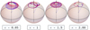Fig. 2 Sample trajectories for the secular evolution of the spin axis of the primary ŝ1, plotted against the unit sphere for different values of κ = ν2 /ν1. The initial conditions are fixed, and shown for the primary as a dashed line from the origin to ŝ1(0). The colours are interpolated between blue and red from initial time to $t_0=50v_1^{-1}$ respectively. The black axis represents the direction of êz. The behaviour for the secondary is analogous, up to a swap of initial conditions and κ → κ−1 = ν1 /ν2.

4 Equilibrium states and stability

A ‘secular’ equilibrium state at time t₀ is a pair of spins defined on an orbital period (ŝ_ı, ŝ₂) : [t₀, t₀ + P_orb] → E₃ × E₃ such that the average change in intrinsic angular momentum is zero: $$\langle \frac{\text{d}{\widehat{s}}_1}{\text{d}t}\rangle \left(t_0\right)=\langle \frac{\text{d}{\widehat{s}}_2}{\text{d}t}\rangle \left(t_0\right)=0.$$(30)

For a purely dipolar magnetic torque, it is clear from Eq. (28) that this condition can only be achieved when the terms of each cross product are either parallel or zero, which we may write more concisely in the form: $$\begin{array}{cccc}ℬ\left({\widehat{s}}_2\right)={\text{λ}}_1{\widehat{s}}_1,& & & ℬ\left({\widehat{s}}_1\right)={\text{λ}}_2{\widehat{s}}_2\end{array}.$$(31)

This corresponds to a singular-value problem, which can be solved with the explicit matrix form of $\overline{ℬ}$ in the orbital-frame basis. Two classes of solutions can be determined from the singular vectors of $\overline{ℬ}$, as described below. In either class, the two spins must be parallel with each other, but they may point in the same direction or in reversed directions. Figure 3 illustrates the full set of equilibrium configurations.

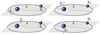Fig. 3 Equilibrium configurations of the spin axes. These correspond to directions that are either inside the orbital plane, in some arbitrary direction (case 1, left column), or orthogonal to the orbital plane (case 2, right column). In each case, the spins may either be parallel (top) or anti-parallel (bottom). As discussed in Sect. 4.2, only the anti-parallel orthogonal configuration (bottom-right) is the only stable scenario.

Case 1. Equilibrium configurations in the orbital plane

The first solution to the singular-value problem corresponds to an equilibrium configuration where the pair of spin axes are both contained inside the orbital plane: $$\begin{array}{cccc}{\widehat{s}}_1={\sigma }_1\widehat{p},& & & {\widehat{s}}_2={\sigma }_2\widehat{p}\end{array},$$(32)

for some unit vector $\widehat{p}$ in the plane of the orbit (i.e. $\widehat{p}\cdot {\widehat{e}}_z=0$). The two unitary parameters (σ₁, σ₂) ∊ {−1, 1} × {−1, 1} describe the relative alignment between the two spins: they can either point in the same direction or in reversed directions. We observe that the set of all pairs (ŝ₁, ŝ₂) which satisfy these conditions at a given moment in time forms a space of dimension 1.

Case 2. Equilibrium configurations orthogonal to the orbital plane

The second solution to the singular-value problem corresponds to a configuration where both spins are orthogonal to the orbital plane - in other words, parallel to the axis ê_z: $$\begin{array}{cccc}{\widehat{s}}_1={\sigma }_1{\widehat{e}}_z,& & & {\widehat{s}}_2={\sigma }_2{\widehat{e}}_z\end{array}.$$(33)

As in the previous case, the spins can be oriented in the same direction or in reverse directions according to the values of σ_ℓ.

4.1 Magnetic interaction energy between two dipoles

The interaction energy between two magnetic dipoles is given by the symmetric expression below (see e.g. Pablo et al. 2019): $$U_B\left({\mu }_1,{\mu }_2\right)=-\frac{{\mu }_0}{4\pi }{\mu }_1\cdot {ℬ}_r\left({\mu }_2\right).$$(34)

We shall denote U_B the ‘instantaneous magnetic energy’. Conversely, one may take the orbital average of U_B, normalising the resulting expression by a positive constant factor: $${\overline{U}}_B\left({\widehat{s}}_1,{\widehat{s}}_2\right)=-{\widehat{s}}_1\cdot \overline{ℬ}\left({\widehat{s}}_2\right).$$(35)

We denote Ū_B the ‘secular magnetic energy’. As can be straightforwardly verified, Ū_B is a constant of motion of the secular system – its time derivative vanishes for any pair (ŝ₁, ŝ₂) ofaxes satisfying (28). Without considering additional forces or dissipation, the orbit-averaged precession system is conservative, and the motion is restricted to some level-curve of constant-energy Ū_B. In astrophysical systems, we expect dissipation due to radiation, tidal forces, and internal frictions to bring the magnetic system to the lower energy states, by exchanging energy until eventually settling into a local minimum of Ū_B. As we shall see, this local minimum corresponds to a state of stability of the physical system.

In Appendix A, we recall that any symmetric bilinear form constrained to the unit n-sphere U : 𝒮_n ×𝒮_n → ℝ is bounded by its largest-magnitude eigenvalue. Applying the principle to the secular magnetic energy (cf. Eq. (35)), one obtains the bounds −2 ≤ Ū_B ≤ 2. The spin configurations in which these bounds are actually attained correspond to ŝ_ℓ along the direction of the associated eigenvector – that is, ŝ_ℓ || ê_z. In fact, such configuration corresponds exactly to the equilibrium states orthogonal to the orbital plane as determined in the previous section (Eq. (33)). In particular, the energy lower bounds are reached in the antiparallel case (σ₂ =−σ₁ which as we shall see, is the most stable equilibrium point. In the following section, we analyse the local stability of all the computed equilibrium states from the standpoint of the Hessian form of Ū_B.

4.2 Stability tests

The stability of each equilibrium configuration can be analysed via the local convexity of the magnetic interaction energy. We evaluate the nature of each of the extrema – minimum, maximum or saddle point – by determining the sign of the Hessian at that point. We remind the reader of its definition.

Consider a real-valued function f of n real variables x = (x₁,…, x_n) with all partial second-order derivatives. The Hessian of f is a matrix-valued function ℋ : ℝⁿ → ℳ_n(ℝ) defined as follows: $$\mathscr{H}\left(x\right)=\left(\begin{array}{ccc}\frac{{\partial }^{2}f}{\partial x_1^2}\left(x\right)& \dots & \frac{{\partial }^{2}f}{\partial x_1\partial x_n}\left(x\right)\\ ⋮& \ddots & ⋮\\ \frac{{\partial }^{2}f}{\partial x_n\partial x_1}\left(x\right)& \dots & \frac{{\partial }^{2}f}{\partial x_n^2}\left(x\right)\end{array}\right)$$(36)

Evaluating the Hessian at some point x ∊ ℝⁿ provides a description of the local convexity of f at that point. If x^* is a critical point (∇f (x^*) = 0) then f can be locally approximated by a quadratic function $$f\left(x^{\ast }+u\right)=f\left(x^{\ast }\right)+\frac{1}{2}{u}^T\mathscr{H}\left(x^{\ast }\right)u+O\left(u^3\right).$$(37)

The Hessian matrix at critical point x^* can be decomposed into its eigenspace in order to obtain the principal directions of curvature. The sign of the corresponding eigenvalues determine whether each direction is stable or unstable.

For the problem at hand, we wish to study the critical points of the secular energy Ū_B as a function of spin direction. For the following, we define the relative alignment between spins ŝ₁ and ŝ₂: $$\sigma ={\sigma }_1{\sigma }_2.$$(38)

Case 1. Equilibrium configurations in the orbital plane

As we have seen, any pair of spin axes which are parallel to each other and contained within the orbital plane will correspond to a secular equilibrium state of the averaged system. Indeed, for any given $\widehat{p}\cdot {\widehat{e}}_z=0$ in Eq. (32) the energy takes the same value ${\overline{U}}_B\left({\sigma }_1\widehat{p},{\sigma }_2\widehat{p}\right)=\sigma$, depending only on the relative orientation of the two spins. The sign of σ = σ₁σ₂ will be positive if the spins are facing the same direction or negative if they are in opposite directions. This invariance with respect to a choice of $\widehat{p}$ in fact reflects the more general axis-symmetry of the system with respect to rotations around the axis ê_z. Simultaneous rotations of both spins will leave the energy expression invariant. In the case of this particular equilibrium configuration, the act of choosing one $\widehat{p}$ lying in the orbital plane over another $\widehat{p}\prime$ corresponds to rotating both spins simultaneously by the angle that takes $\widehat{p}\prime \mapsto \widehat{p}$. The set of all unit vectors $\widehat{p}$ in the orbital plane corresponds to a one-dimensional level-set of constant energy (a circle). To study the stability of this level-set we can reduce the degrees of freedom of the system from four (two for each spin axis, i.e. 𝒮₂ × 𝒮₂) to three (by removing the rotational degree of freedom). In this reduced three-dimensional manifold, the circle becomes a point, and the remaining three directions of the tangent space determine the convexity of the energy.

As a first step, we consider the spins parametrised in spherical coordinates, $${\widehat{s}}_{\ell }=\left(\cos {\psi }_{\ell }\sin {\theta }_{\ell },\sin {\psi }_{\ell }\sin {\theta }_{\ell },\cos {\theta }_{\ell }\right),$$(39)

with azimuth ψ_ℓ and angle θ_ℓ measured from the north pole. In these coordinates, the secular energy takes the form $${\overline{U}}_B=2\cos {\theta }_1\cos {\theta }_2-\cos \left({\psi }_1-{\psi }_2\right)\sin {\theta }_1\sin {\theta }_2.$$(40)

As discussed above, we can see clearly that simultaneous rotations in the azimuth ψ₁ and ψ₂ do not affect the energy. We can therefore look at the difference ψ₁ – ψ₂ := ∆ψ and discard the redundant degree of freedom ψ₁ + ψ₂. At the equilibrium, the polar angles are θ₁ = θ₂ = π/2, and the azimuth is either ∆ψ = 0 or ∆ψ = π. We consider therefore the three directions of the tangent space of this reduced manifold. In this case, the Hessian matrix of the energy Ū_B with respect to the three variables (∆ψ, θ₁, θ₂) has value: $${\mathscr{H}}_1=\left(\begin{array}{lll}\sigma \hfill & 0\hfill & 0\hfill \\ 0\hfill & \sigma \hfill & 2\hfill \\ 0\hfill & 2\hfill & \sigma \hfill \end{array}\right)$$(41)

The sign of σ = ±1 corresponds to the two cases of the spin directions being aligned or anti-aligned. For either sign, the Hessian has both positive and negative eigenvalues (−1, 1 and 3σ). This implies a saddle point, which is unstable.

Case 2. Equilibrium configurations orthogonal to the orbital plane

In the second case, we consider both spins to be orthogonal to the plane of the orbit. The spin axes ŝ_ℓ therefore will be lying in the north or south pole of their corresponding unit spheres. A natural choice of coordinates for each spin in the neighbourhood of the poles is the Cartesian pair x_ℓ, y_ℓ, which with the unit-norm condition gives $${\widehat{s}}_{\ell }=\left(x_{\ell },y_{\ell },{\sigma }_{\ell }\sqrt{1-x_{\ell }^2-y_{\ell }^2}\right)$$(42)

In these coordinates, the secular magnetic energy can be expressed in the form: $${\overline{U}}_B=-x_1{x}_2-y_1{y}_2+2\sigma \sqrt{1-x_l^2-y_l^2}\sqrt{1-x_2^2-y_2^2}.$$(43)

The corresponding basis for the tangent space is the coordinate basis dx_ℓ and dy_ℓ. With respect to these coordinates the Hessian of the energy takes the values: $${\mathscr{H}}_2=-\left(\begin{array}{llll}2\sigma \hfill & 0\hfill & 1\hfill & 0\hfill \\ 0\hfill & 2\sigma \hfill & 0\hfill & 1\hfill \\ 1\hfill & 0\hfill & 2\sigma \hfill & 0\hfill \\ 0\hfill & 1\hfill & 0\hfill & 2\sigma \hfill \end{array}\right)$$(44)

The nature of the eigenvalues of the Hessian change according to the sign of σ: when the spins are aligned (σ = +1), the Hessian is negative definite, with eigenvalues {−3, −3, −1, −1}, implying a point of maximum energy and therefore instability; when the spins are in opposing directions (σ = −1), the eigenvalues are {1, 1, 3, 3} and the Hessian is positive definite, which implies a point of minimum energy and hence stability.

This suggests that given enough time and in the absence of stronger torques, magnetically interacting systems will naturally converge towards the stable anti-aligned orthogonal configuration. The timescale of this convergence will depend on the strength of the dissipation effects involved.

4.3 Solutions near equilibrium

In Appendix B, we determine solutions near the stable equilibrium state. These solutions can be plugged in to derive complete secular orbital dynamics on systems which present strong magnetic torques, such as WD or NS binaries in the context of gravitational wave emission (for further details, see e.g. Bourgoin et al. 2022; Lira et al. 2022). We present below the main results:

The spins can be decomposed as ŝ_ℓ = x_ℓ ê_x + y_ℓ ê_y + z_ℓ ê_z, where the orbital-plane components satisfy $$x_{\ell }\left(t\right)={\rho }_{\ell }^{+}\cos \left({\omega }_p^{+}t+{\varphi }_{\ell }^{+}\right)+{\rho }_{\ell }^{-}\cos \left({\omega }_p^{-}t+{\varphi }_{\ell }^{-}\right),$$(45a) $$y_{\ell }\left(t\right)={\rho }_{\ell }^{+}\sin \left({\omega }_p^{+}t+{\varphi }_{\ell }^{+}\right)+{\rho }_{\ell }^{-}\sin \left({\omega }_p^{-}t+{\varphi }_{\ell }^{-}\right),$$(45b)

and the orthogonal component satisfies $$Z_1\left(t\right)=\frac{1}{2v_2}\left(\zeta +{\overline{Q}}_z+{\rho }_z\cos \left({\omega }_{z}t+{\varphi }_z\right)\right),$$(46a) $$Z_2\left(t\right)=\frac{1}{2v_1}\left(\zeta -{\overline{Q}}_z-{\rho }_z\cos \left({\omega }_{z}t+{\varphi }_z\right)\right),$$(46b)

with real parameters ${\rho }_{\ell }^{\pm }$, ${\varphi }_{\ell }^{\pm }$, ρ_z, ϕ_z, dependent on initial conditions. The expressions of the constants ζ and ${\overline{Q}}_z$ and the frequencies ω_z, ${\omega }_p^{+}$, and ${\omega }_p^{-}$ are given in the appendix.

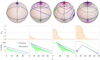Fig. 4 Evolution of the binary system in a secular timescale with dissipation introduced. Each column corresponds to a given initial condition from Table 2, chosen in a neighbourhood of an equilibrium point. On the top row: the trajectory of each spin axis ŝℓ is plotted against the unit sphere, in blue for the primary and green for the secondary. Colours are interpolated towards red from initial time to final time of convergence. Initial conditions for the spin axes are portrayed as dashed lines from the origin to ŝℓ (0). The orbital plane is represented in a darker shade with black contours, and the axis êz as a vertical black arrow. On the middle row: the secular magnetic interaction energy. On the bottom row: the angular distance of each spin axis with respect to the stable equilibrium point (êz, − êz).

5 Numerical validation

We present in this section a numerical verification of the results that were obtained in Sect. 4. In the first part, we demonstrate the derived (in-)stability of each equilibrium configuration. In the second part, we compare the obtained analytical solutions to numerical integration, in the neighbourhood of the stable equilibrium.

5.1 Stability of the equilibrium configurations

We artificially introduce dissipation into the dynamics of the secular system and numerically show that it is driven towards the stable states. Such a dissipative effect must preserve the norm condition on unit vectors and manifest as a friction when orientation changes. For this we include a time-delay term into the magnetic field that is felt by each companion star. By our previous arguments in Sect. 3, it is direct to see that this term will propagate to the secular scale as follows: $$\langle \frac{\text{d}{\widehat{s}}_1}{\text{d}\tau }\rangle \left(\tau \right)={\widehat{s}}_1\left(\tau \right)\times \overline{ℬ}\left({\widehat{s}}_2\left(\tau -\text{Δ}\tau \right)\right),$$(47a) $$\langle \frac{\text{d}{\widehat{s}}_2}{\text{d}\tau }\rangle \left(\tau \right)=\kappa {\widehat{s}}_2\left(\tau \right)\times \overline{ℬ}\left({\widehat{s}}_1\left(\tau -\text{Δ}\tau \right)\right),$$(47b)

where we have used the re-scaled dimensionless time $\tau \mapsto v_1^{-1}\tau$ and κ = ν₂/ν₁ = s₁/s₂ presented at the end of Sect. 3. For convenience, we consider the delay to be an order of magnitude smaller than the average torque timescale, Δτ ~ 0.1 κ^−1/2. This provides us with dissipative effects visible on the simulation timescales.

In order to assess stability, we consider two metrics: the secular magnetic interaction energy Ū_B (see Eq. (35)); and the angular distance to the stable equilibrium point (ê_z, − ê_z), which we define as: $$d_1=\arg \left({\widehat{s}}_1,+{\widehat{e}}_z\right),$$(48a) $$d_2=\arg \left({\widehat{s}}_2,-{\widehat{e}}_z\right),$$(48b)

where arg(u, v) = arctan2 (|u ×v|, u · v) is the angle between any two vectors u and v.

The dimensionless system is then integrated until convergence, for four sets of initial spin conditions (Table 2), and with spin ratio κ = 0.3. Each initial condition corresponds to an unstable equilibrium state plus a small perturbation of the order of ~1º. For completeness, we also include a perturbation of the stable state (~10º). The resulting trajectories are plotted in Fig. 4, together with the time evolution of the secular energy Ū_B and of the angular distances d₁ and d₂. Even for a small initial angular perturbation, the spin axes diverge from their original unstable equilibrium and converge towards the stable, anti-aligned orthogonal configuration.

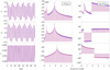Fig. 5 Comparison between the analytical precession model (blue) and numerical integration (red), close to stable equilibrium. On the leftmost column: the components of the spin of the primary, in the time domain. The corresponding Discrete Fourier Transform ℱ{ŝ1} is given in absolute value (power spectrum in decibels, middle column), and in complex argument (rightmost column). The time and frequency axes are expressed in the re-scaled dimensionless units.

5.2 Solutions near equilibrium

In this part, we present a brief application of the analytical solutions of the secular equations that were exposed in Sect. 4.3. The equations are expressed in dimensionless time, and we adopt a spin ratio of κ = 0.3. The following initial conditions are considered (polar coordinates): inclinations θ₁ = 10° and θ₂ = 172.5° from the north pole, and azimuths ψ₁ = 0 and ψ₂ = 50°. Figure 5 compares the obtained analytical expression of the primary to numerical integration, decomposed in the Cartesian basis ŝ₁ (τ) = x₁ (τ) ê_x + y₁ (τ) ê_y + z₁ (τ) ê_z. Matching peaks can be observed in the power spectra of both solutions, at the obtained angular frequencies (in dimensionless units) ${\omega }_p^{-}=0.47$ rad and ${\omega }_p^{+}=1.86$ rad for the orbital components (x₁, y₁), and at ω_z = 2.34 rad for the orthogonal component z₁ (cf. Appendix B).

6 Discussion

We have so far defined the concept of a secular equilibrium state and applied it to obtain the equilibrium dynamics of binary systems with two magnetic components. In this section, we begin by discussing the fine points between secular and instantaneous equilibrium. Then, we apply our results to a real astrophysical scenario, the ϵ-Lupi magnetic binary.

6.1 Comparison between instantaneous and secular equilibrium states

In Sect. 4, we defined the secular equilibrium as the spin configurations where the net torque over an orbital period is effectively zero. These states contrast with the instantaneous equilibrium, the configurations of zero torque on the instantaneous precession system (Eq. (13)). In the latter scenario, the spin dynamics are considered at a single moment in time and at a fixed orbital position. When orbital motion is introduced, an instantaneous equilibrium state may be destabilised. This can be seen in the following manner. We consider a bounded orbit parametrised by the osculating true anomaly f = f (t). Expressing the spins in spherical coordinates, the instantaneous magnetic energy U_B (Eq. (34)) takes the form: $$U_B\left(t\right)=\frac{{\mu }_0{\mu }_1{\mu }_2}{4\pi r^3}\left({\widehat{\mu }}_1\cdot {\widehat{\mu }}_2-3\sin {\theta }_1\sin {\theta }_2\cos \left({\psi }_1-f\left(t\right)\right)\cos \left({\psi }_2-f\left(t\right)\right)\right).$$(49)

Whereas the dot-product term on the right-hand side is invariant to an orbital translation of the bodies, the cosine terms oscillate with the orbital dynamics. We take two instants within the same orbital revolution, t₁ and t₂ such that the true anomaly at each instant equals f (t₁) = (ψ₁ + ψ₂)/2 and f (t₂) = (ψ₁ + ψ₂ + π)/2. Then the difference in energy between those two instants is roughly $$U_B\left(t_2\right)-U_B\left(t_1\right)\sim \frac{3{\mu }_0{\mu }_1{\mu }_2}{4\pi a^3}\sin {\theta }_1\sin {\theta }_2,$$(50)

where we have substituted r ~ a. We conclude that instantaneous equilibrium positions will indeed develop large energy oscillations in the timescale t ~ P_orb, particularly when the polar angle θ_ℓ is large (i.e. spin axes close to orbital plane alignment). For rapidly orbiting systems, this energy fluctuation occurs very quickly and destabilises the equilibrium of the point.

There is a direct analogy between the states of secular equilibrium and those of instantaneous equilibrium. We recall the expression of the secular magnetic energy: $$\begin{array}{cc}{\overline{U}}_B=-{\widehat{s}}_1\cdot \overline{ℬ}\left({\widehat{s}}_2\right),& \overline{ℬ}\end{array}=\mathbb{I}-3{\widehat{e}}_z\otimes \underset{\_}{{\widehat{e}}_z}.$$

Such expression has been normalised by the positive constant µ₀µ₁µ₂/8πb³ as discussed in Sect. 4. We similarly normalise the expression of the instantaneous magnetic energy (cf. Eq. (34)) by the scalar µ₀µ₁µ₂/4πr³ and obtain: $$\begin{array}{cc}{U}_B\propto +{\widehat{s}}_1\cdot {\widetilde{ℬ}}_r\left({\widehat{s}}_2\right),& {\widetilde{ℬ}}_r=\mathbb{I}\end{array}-3\widehat{r}\otimes \underset{\_}{\widehat{r}}.$$

We observe that the secular averaging procedure effectively produced a flip in the sign of the energy as well as a switch $\widehat{r}\leftrightarrow {\widehat{e}}_z$. Analogously to how the secular equilibrium states of the binary are given by the singular vectors of $\overline{ℬ}$ (cf. Sect. 4), the instantaneous states are given by the singular vectors of ${\widetilde{ℬ}}_r$. Consequently, each state of instantaneous equilibrium has a secular counterpart. These correspond to spin axes aligned with the radial direction $\widehat{r}$ (resp. ê_z) or perpendicular to $\widehat{r}$ (resp. ê_z). The stability of each state depends on the local convexity of the energy U_b (resp. U_b). We present in Table 3 a comparison between the obtained states for the two types of equilibrium.

6.2 ϵ-Lupi

We consider as a potential application case the ϵ-Lupi inner binary system. ϵ-L·upi is a ternary system composed of two close-range B-type companions Aa and Ab, plus a third distant companion dubbed ϵ-L·upi B. Both stars of the ϵ-L·upi A inner system are magnetic, making it the first and only currently known massive binary that has two magnetic components. Furthermore, the field of each star can be captured by a dipolar model with axes roughly parallel to the spins (Shultz et al. 2015). The system also has a short orbital period of P_orb ~ 4.56 d, making it an excellent example to apply our model. Pablo et al. (2019), Uytterhoeven et al. (2005) obtained estimates for relevant stellar and orbital parameters, from which we adopt the values for the semi-major axis a = 29.5 R_⊙, eccentricity of e = 0.28, inclination ι = 21°, stellar masses of m₁ = 9.0 M_⊙ for the primary and m₂ = 7.9 M_⊙ for the secondary, and radii R₁ = R₂ = 4.5 R_⊙.

Shultz et al. (2015) reports a dipolar field strength of at least $B_1^{\text{p}}=600$ G and $B_1^{\text{p}}=900$ G at the surface poles of the star, and projected rotational velocities at the equator v₁ sin i₁ = 37 km s⁻¹ for the primary and v₂ sin i₂ = 27 km s⁻¹ for the secondary. By adopting the rotational inclination for each star equal to the orbital plane inclination ι ~ 21°, we obtain rotational periods of the order of P₁ = 2.2 d and P₂ = 3.0 d.

From these physical parameters we may calculate the corresponding dimensionless ratios. The impact of figure effects can be assessed via ${\gamma }_{\ell }^{\text{fig}}=2\times 10J_2^{\ell }$, whereas for tides ${\gamma }_1^{\text{tide}}=2.5\times {10}^8\left(k_2^1/Q_1\right)$ and ${\gamma }_2^{\text{tide}}=3.5\times {10}^8\left(k_2^2/Q_2\right)$. These expressions suggest that if ϵ-·upi is both highly symmetrical with $J_2^{\ell }\lesssim 6\times {10}^{-11}$, and has tidal parameters $k_2^{\ell }/Q_{\ell }\lesssim 3\times {10}^{-9}$, then the system's rotation is likely driven by magnetism. In this case, the smallness of η = 5 × 10⁻¹² and ϵ = 4 × 10⁻¹¹ predict that the system will be driven towards the secular stable equilibrium in a timescale proportional to energy dissipation rates. This outcome corresponds well to the expected state of ϵ-·upi based on observational data (Pablo et al. 2019).

7 Conclusions

This paper has presented an analysis of the secular precession dynamics of binary systems under pure magnetic dipole-dipole interactions, considering an effective description with orbit-averaged motion. In particular, we have supposed spin-dipole alignment, perfect sphericity and tidal rigidity, and then derived criteria for assessing the validity of these assumptions, as well as the relative strengths of magnetic dipole interactions, tidal torques, and figure effects. We have shown that this effective long-term description predicts a set of states of secular equilibrium which confront the traditional states of instantaneous magnetic equilibrium, where orbital dynamics are in fact neglected. Indeed, we have determined that there is a single secular state that is globally stable, corresponding to the configuration ±(ê_z, −ê_z) where the spin axes are reversed with respect to each other and orthogonal to the orbital plane. Conversely, the instantaneous state of radial alignment $\pm \left(\widehat{r},\widehat{r}\right)$ is in fact only momentarily stable, since the orbital motion generates energy fluctuations and destabilises the configuration. Our work can also be used to derive the long-term evolution of binary orbits providing an expected spin evolution in the absence of strong additional torques.

Our results hold for typical early-type MMS (such as the observed ϵ-Lupi system), WD, and NS binaries hosting dipolar fossil-like fields, where we expect long-term convergence towards the secularly stable state. Another interesting case of application is that of M dwarfs. For masses lower than 0.35M_⊙, M dwarfs are fully convective, unlike any other main-sequence stars, which renders the dynamo-driven topology unique (e.g. Dobler et al. 2006; Browning 2008). These low- and mid-mass M dwarfs are possible targets of application for our formalism since their magnetic fields often display intense dipolar components (e.g. Donati et al. 2008), although intermittent higher-order multipolar components might also be present (e.g. Kochukhov 2021, and references therein). Moreover, they have been observed forming binaries with two magnetic components (e.g. Kochukhov & Lavail 2017; Kochukhov & Shulyak 2019). An interesting example of such binary systems is that of the YY Gem system (Kochukhov & Shulyak 2019), where each star has both dipolar and multipolar components. The Zeeman-Doppler imaging analysis indeed revealed moderately complex global fields with a typical strength of 200-300 G, with dipolar components that are anti-aligned as predicted for fossil-type fields. These considerations hint that our work might be applied to any type of dipolar magnetic fields, either of fossil origin or triggered by a dynamo action, as long as its variation timescales are longer than the precession timescales. However, as mentioned in Kochukhov & Shulyak (2019), the Zeeman intensification analysis suggests that the global fields of YY Gem may only comprise a few percent of their total magnetic fields, which highlights the need to consider multipoles in future studies. In addition, we point out that in typical M dwarf binary systems, gravitational interactions may control the orientation of the spins themselves. We can in fact compute (for a typical magnetic M dwarf: m ~ 0.35 M_⊙, B ~ 1 kG) the dimensionless parameters that measure the strength of extended-body gravitational interactions with respect to magnetic torques: γ_fig = 6 × 10¹¹ J₂ and γ_tides = 7 × 10⁷k₂/Q (Eqs. (9), (11)). Subsequently, we obtain the (quite tight) cutoffs J₂ ≤ 10⁻¹² for the dimensionless quadrupole moment (Eq. (10)), and k₂/Q ≤ 10⁻⁸ for the tidal parameters (Eq. (12)), as the necessary parameters for magnetism to control the spin evolution.

Another key assumption from this work that warrants discussion is the alignment between the spin and magnetic axes of each star, since many misaligned systems are observed in nature (e.g Shultz et al. 2019). In the case where the spin and magnetic dipole are anti-aligned (µ_ℓ < 0 in Eq. (5)), our general results still hold but spin directions must be flipped accordingly in the equations. More generally, this alignment constraint must be relaxed in future studies to explore the more general scenario of misaligned spin and magnetic axes. Assuming a rigid description where the magnetic axes rotate around the spins, a potentially direct case could be when the stellar rotation period P_ℓ is much shorter than the orbital period P_orb. In such regime, the problem may be hierarchically split into three distinct timescales P_ℓ ≪ P_orb ≪ τ, where τ is the ‘spin precession timescale’ as described in Sect. 2 (Eq. (15)). The dynamics could then be formulated as an effective description when seen from the longer orbital timescale P_orb, potentially reducing to the one explored in this work. Accordingly, one could expect our main results to still hold.

Further extensions of this work will also include abandoning the magnetostatic description and considering internal coupling of the fields with matter (Campbell 2018). Finally, the precession dynamics and equilibrium states of the system may be investigated by directly taking into account not only magnetic forces but also competing figure effects and dynamical tides (see example of such combined study in Ahuir et al. 2021).

Acknowledgements

C.A. acknowledges the joint finantial support of Centre National d’Études Spatiales (CNES) and École Doctorale Astronomie et Astrophysique d’Île-de-France (ED127 AAIF). This work was also supported by the Programme National GRAM, by PNPS (CNRS/INSU), by INP and IN2P3 co-funded by CNES, and by CNES LISA grants at CEA/IRFU. Authors are also grateful to S. Bouquillon for fruitful discussions. We are thankful to the anonymous reviewer for their constructive comments, which allowed us to improve our article.

Appendix A Optimisation of bilinear forms

In this appendbix we recall the variational characterisation of the singular value decomposition. Consider the bilinear form U taking two unit vectors U : 𝒮_n × 𝒮_n → ℝ, represented under a basis {ê₁,…, ê_n} via some matrix U_ij: $$U\left(\widehat{u},\widehat{\upsilon }\right)=U_{ij}{u}^i{\upsilon }^j,$$(A.1)

where û = uⁱê_i, $\widehat{\upsilon }={\upsilon }^i{\widehat{e}}_i$, and sum over repeated indices is presupposed.

Since U is continuous on the compact domain 𝒮_n × 𝒮_n, it attains both a maximum and minimum value. Indeed, consider the Lagrange function $$g\left(\widehat{u},\widehat{\upsilon }\right)=U\left(\widehat{u},\widehat{\upsilon }\right)-{\lambda }_1\left(\widehat{u}\cdot \widehat{u}-1\right)-{\lambda }_2\left(\widehat{\upsilon }\cdot \widehat{\upsilon }-1\right),$$(A.2)

with multipliers λ₁ and λ₂. The extrema û_* and ${\widehat{\upsilon }}_{\ast }$, necessarily satisfy the stationary condition $\nabla g\left({\widehat{u}}_{\ast },{\widehat{\upsilon }}_{\ast }\right)=0$, which implies that for any tangent vectors h₁, h₂, $$U\left(h_1,{\widehat{\upsilon }}_{\ast }\right)=2{\lambda }_1{\widehat{\upsilon }}_{\ast }\cdot h_1,$$(A.3a) $$U\left({\widehat{u}}_{\ast },h_2\right)=2{\lambda }_2{\widehat{\upsilon }}_{\ast }\cdot h_2.$$(A.3b)

From the matrix representation of U [Eq. (A.1)], we see that the solutions û_* and ${\widehat{\upsilon }}_{\ast }$ correspond respectively to the left and right singular vectors of U_ij — that is, the unique set of vectors that satisfy $$\begin{array}{llll}{U}_{ij}{u}_{\ast }^i=\lambda {\upsilon }_{\ast }^i\hfill & \hfill & \hfill & U_{ij}{\upsilon }_{\ast }^i=\lambda u_{\ast }^i\hfill \end{array}$$(A.4a)

where λ = 2λ₁ = 2λ₂ is the corresponding singular value of U_ij.

It is direct to see that the attained value $U_{\ast }=U\left({\widehat{u}}_{\ast },{\widehat{\upsilon }}_{\ast }\right)=\lambda$. From all singular-vector pairs $\left({\widehat{u}}_{\ast },{\widehat{\upsilon }}_{\ast }\right)$, the global maximum (or minimum) of U is therefore reached by the candidate pair that has the highest (or lowest) corresponding singular value λ. We note that whenever U is symmetric, the singular vectors and eigenvectors of U_ij coincide, and the singular values are equal to the magnitude of the eigenvalues.

Appendix B Linearised solutions

In this section, we formally derive secular solutions to the spin-spin equations, $$\langle \frac{\text{d}{\widehat{s}}_1}{\text{d}t}\rangle =-v_1\overline{ℬ}\left({\widehat{s}}_2\right)\times {\widehat{s}}_1,$$(B.1a) $$\langle \frac{\text{d}{\widehat{s}}_2}{\text{d}t}\rangle =-v_2\overline{ℬ}\left({\widehat{s}}_2\right)\times {\widehat{s}}_2,$$(B.1b)

and $$\overline{ℬ}=\mathbb{I}-3{\widehat{e}}_z\otimes \underset{\_}{{\widehat{e}}_z},$$

in a neighbourhood of the stable equilibrium point. The solution obtained here is in fact more generally valid for any configuration close to the poles (ŝ₁, ŝ₂) ≈ (σ₁ê_z, σ₂ê_z), including the unstable aligned orthogonal case (see Sect. 4). As in the main text, we consider two indices ℓ, m ∊ {1, 2}, with m ≠ ℓ, representing the pair of binaries permuted in some order.

In order to solve the system (B.1), we take advantage of the axial symmetry of the physical system around ê_z. We split the Euclidean vector space E₃ into an orbital plane Π = {x ê_x + y ê_y; (x,y) ∊ ℝ²} plus a normal line Λ = {zê_z; z ∊ ℝ} such that E₃ = Π ⊕ Λ. Rotations of the plane Π leave (B.1) invariant.

We identify the line Λ with the reals and the orbital plane Π with the complex plane by introducing the linear isomorphism Φ : Π × Λ → ℂ × ℝ, which satisfies²: $$\text{Φ}\left(x{\widehat{e}}_{\text{X}}+y{\widehat{e}}_y+z{\widehat{e}}_{\text{Z}}\right)=\left(x+iy,z\right),$$(B.2)

where i is the imaginary number. Eq. (B.1) can be expressed in the space ℂ × ℝ by declaring a new set of spin variables, which we define uniquely from Φ(ŝ_ℓ) = (p_ℓ, z_ℓ). More explicitly, p_ℓ corresponds to the orbital component of ŝ_ℓ, and z_ℓ corresponds to the projection of ŝ_ℓ on the basis element ê_z: $$p_{\ell }=\left({\widehat{s}}_{\ell }\cdot {\widehat{e}}_X\right)+\text{i}\left({\widehat{s}}_{\ell }\cdot {\widehat{e}}_y\right),$$(B.3) $$z_{\ell }=\left({\widehat{s}}_{\ell }\cdot {\widehat{e}}_Z\right).$$(B.4)

This identification allows us to leverage the rotational symmetries of Π through the algebraic structures of the complex numbers. In particular, through the isomorphism, vector dot-and cross-products in E₃ can be described in terms of complex multiplication and conjugation³.

For each body, we obtain the new and equivalent form of the spin precession equations: $$\frac{\text{d}{p}_{\ell }}{\text{d}t}=\text{i}{\nu }_{\ell }\left(z_{\ell }{p}_{\text{m}}+2z_{\text{m}}{p}_{\ell }\right),$$(B.5) $$\frac{\text{d}{z}_{\ell }}{\text{d}t}={\nu }_{\ell }\mathfrak{J}\mathfrak{m}\left(p_{\ell }^{\ast }{p}_{\text{m}}\right),$$(B.6)

where 𝔑𝔢, ℑ𝔪 are the real and imaginary parts, and the operation p → p^* denotes complex conjugation. These equations are coupled by the four parameters (p₁, p₂, z₁, z₂) with values in ℂ² × ℝ², for a total dimensionality of 6. As discussed in Sect. 3, two degrees of freedom are redundant, constrained by the unit-norm conditions $${\left|p_{\ell }\right|}^2+z_{\ell }^2=1,$$(B.7)

and the magnetic interaction energy defines a conserved quantity: $${\overline{U}}_B=2z_{\ell }{z}_{\text{m}}-\Re e\left(p_{\ell }^{\ast }{p}_{\text{m}}\right).$$(B.8)

The anti-symmetry of the equation (B.6) with respect to a swap of indices ℓ ↔ m allows us to determine another first integral for the problem — namely, the z-component of the total intrinsic angular momentum, S_z = s₁z₁ + s₂z₂. We introduce the quantity: $$\zeta ={\nu }_2{z}_1\left(t\right)+{\nu }_1{z}_2\left(t\right)=\frac{{\mu }_0{\mu }_1{\mu }_2}{8\pi a^3{\left(1-e^2\right)}^{3/2}}\frac{1}{s_1{s}_2}{S}_z.$$(B.9)

Since for any two complex numbers ℑ𝔪(u^*v + v^*u) = 0, it follows that the derivative of ζ vanishes. We also introduce the anti-symmetric spin: $$Q_z\left(t\right)=v_2{z}_1\left(t\right)-v_1{z}_2\left(t\right),$$(B.10)

which is not a conserved quantity.

The spins of the two bodies can be decoupled in Eqs. (B.5) and (B.6) via differentiation and substitution of the constraints. We obtain the second-order system of equations below, purely in terms of the variables p₁, p₂, and Q_z: $$\frac{{\text{d}}^2{p}_1}{\text{d}{t}^2}={\alpha }_{+}\frac{\text{d}{p}_1}{\text{d}t}+{\beta }_{-}{p}_1,$$(B.11) $$\frac{{\text{d}}^2{p}_2}{\text{d}{t}^2}={\alpha }_{-}\frac{\text{d}{p}_2}{\text{d}t}+{\beta }_{+}{p}_2,$$(B.12) $$\frac{{\text{d}}^2{Q}_z}{\text{d}{t}^2}=a-b{Q}_z+3Q_z^3,$$(B.13)

with α+, α_,β+,β_ four functions defined via $${\alpha }_{\pm }\left(t\right)=2\text{i}\zeta \pm \frac{1}{\zeta +Q_z\left(t\right)}\frac{\text{d}{Q}_z}{\text{d}t}\left(t\right),$$(B.14) $${\beta }_{\pm }\left(t\right)=\frac{3}{4}\left({\zeta }^2-Q_z^2\left(t\right)\right)\pm \frac{2\text{i}\zeta }{\zeta +Q_z\left(t\right)}\frac{\text{d}{Q}_z}{\text{d}t}\left(t\right),$$(B.15)

and the constants a ∊ ℝ, b ∊ ℝ⁺ given by $$\begin{array}{cc}a=\left(v_2^2-v_1^2\right)\zeta ,& b=v_1^2+v_2^2+4{\overline{U}}_B{v}_1{v}_2-\frac{3}{2}{\zeta }^2.\end{array}$$(B.16)

To solve the full system of equations, we must first solve for Q_z and then plug the obtained solution in the expression of α± and β± in order to determine p₁ and p₂. In fact, there is an exact analytical solution for Q_z in terms of elliptic functions. The resulting expression for Q_z is somewhat lengthy, and subsequently solving (B.11), (B.12) in this scenario proves to be challenging. Instead, we opt to present simpler and physically meaningful expressions for all the parameters, with domain of validity close to the poles.

We consider the expansion of Eqs. (B.11)–(B.13) around some origin ${\overline{Q}}_z$, with $Q_z\left(t\right)={\overline{Q}}_z+\delta Q_z\left(t\right)$. For a good choice of ${\overline{Q}}_z$, the resulting system may be truncated at low orders in δQ_z to yield low-order solutions $Q_z^{\left(0\right)}$, $Q_z^{\left(1\right)}$, etc. In particular, we constrain ${\overline{Q}}_z$ to the domain of Q_z by choosing ${\overline{Q}}_z=Q_z\left(t_0\right)$ for a reference time t₀. The error incurred from this expansion will depend on the largeness of the variations δQ_z — which are assumed small in the neighbourhood of the poles. Indeed, we consider some arbitrary spin variation from t0 to t, namely δŝ_ℓ(t) = ŝ_ℓ(t) − ŝ_ℓ(t₀). Due to the geometry of the unit sphere, this variation will propagate along the z component to some |δz_ℓ(t)| ≤ |δŝ_ℓ(t)| sin θ_ℓ ≤ 2 sin θ_ℓ, where θ_ℓ is the maximum attained polar inclination, that is, sin θ_ℓ = sup_t |ŝ_ℓ(t) · ê_z|. For a solution close to the poles, the polar angle θ_ℓ is assumed a small parameter. In this case, the perturbation δQ_z(t) = v₂δz₁(t) − v₁δz₂(t) will also remain similarly bounded. With these considerations, we present below the solutions for low orders of δQ.

References

- Achilleos, N., & Wickramasinghe, D. T. 1989, ApJ, 346, 444 [NASA ADS] [CrossRef] [Google Scholar]
- Ahuir, J., Strugarek, A., Brun, A. S., & Mathis, S. 2021, A&A, 650, A126 [NASA ADS] [CrossRef] [EDP Sciences] [Google Scholar]
- Akgün, T., Reisenegger, A., Mastrano, A., & Marchant, P. 2013, MNRAS, 433, 2445 [Google Scholar]
- Alecian, E., Neiner, C., Wade, G. A., et al. 2014, Proc. Int. Astron. Union, 9, 330 [CrossRef] [Google Scholar]
- Amaro-Seoane, P., Audley, H., Babak, S., et al. 2017, Laser Interferometer Space Antenna (USA: NASA) [Google Scholar]
- Aurière, M., Wade, G. A., Silvester, J., et al. 2007, A&A, 475, 1053 [NASA ADS] [CrossRef] [EDP Sciences] [Google Scholar]
- Bagnulo, S., & Landstreet, J. D. 2021, MNRAS, 507, 5902 [NASA ADS] [CrossRef] [Google Scholar]
- Beuermann, K., Euchner, F., Reinsch, K., Jordan, S., & Gänsicke, B. T. 2007, A&A, 463, 647 [NASA ADS] [CrossRef] [EDP Sciences] [Google Scholar]
- Borra, E. F., Landstreet, J. D., & Mestel, L. 1982, ARA&A, 20, 191 [NASA ADS] [CrossRef] [Google Scholar]
- Bourgoin, A., Le Poncin-Lafitte, C., Mathis, S., & Angonin, M.-C. 2022, Phys. Rev. D, 105, 124042 [NASA ADS] [CrossRef] [Google Scholar]
- Braithwaite, J. 2008, MNRAS, 386, 1947 [Google Scholar]
- Braithwaite, J. 2009, MNRAS, 397, 763 [NASA ADS] [CrossRef] [Google Scholar]
- Braithwaite, J., & Cantiello, M. 2013, MNRAS, 428, 2789 [NASA ADS] [CrossRef] [Google Scholar]
- Braithwaite, J., & Nordlund, Å. 2006, A&A, 450, 1077 [NASA ADS] [CrossRef] [EDP Sciences] [Google Scholar]
- Braithwaite, J., & Spruit, H. C. 2004, Nature, 431, 819 [Google Scholar]
- Bromley, B. C., & Kenyon, S. J. 2022, AJ, 164, 229 [NASA ADS] [CrossRef] [Google Scholar]
- Browning, M. K. 2008, ApJ, 676, 1262 [Google Scholar]
- Brun, A. S., & Browning, M. K. 2017, Liv. Rev. Sol. Phys., 14, 4 [Google Scholar]
- Brun, A., Strugarek, A., Noraz, Q., et al. 2022, ApJ, 926, 21 [NASA ADS] [CrossRef] [Google Scholar]
- Campbell, C. G. 2018, Magnetohydrodynamics in Binary Stars (Berlin: Springer), 456 [Google Scholar]
- Carrier, F., North, P., Udry, S., & Babel, J. 2002, A&A, 394, 151 [NASA ADS] [CrossRef] [EDP Sciences] [Google Scholar]
- Carvalho, G. A., Anjos, R. C. D., Coelho, J. G., et al. 2022, ApJ, 940, 90 [NASA ADS] [CrossRef] [Google Scholar]
- Charbonneau, P., & MacGregor, K. B. 2001, ApJ, 559, 1094 [NASA ADS] [CrossRef] [Google Scholar]
- Commerçon, B., Hennebelle, P., Audit, E., Chabrier, G., & Teyssier, R. 2010, A&A, 510, L3 [NASA ADS] [CrossRef] [EDP Sciences] [Google Scholar]
- Cumming, A. 2002, MNRAS, 333, 589 [NASA ADS] [CrossRef] [Google Scholar]
- Damiani, C., & Lanza, A. F. 2015, A&A, 574, A39 [NASA ADS] [CrossRef] [EDP Sciences] [Google Scholar]
- de Mink, S. E., Sana, H., Langer, N., Izzard, R. G., & Schneider, F. R. N. 2014, ApJ, 782, 7 [Google Scholar]
- Dobler, W., Stix, M., & Brandenburg, A. 2006, ApJ, 638, 336 [NASA ADS] [CrossRef] [Google Scholar]
- Donati, J. F., & Landstreet, J. D. 2009, ARA&A, 47, 333 [Google Scholar]
- Donati, J. F., Morin, J., Petit, P., et al. 2008, MNRAS, 390, 545 [Google Scholar]
- Duez, V. 2011, Astron. Nachr., 332, 983 [Google Scholar]
- Duez, V., Braithwaite, J., & Mathis, S. 2010, ApJ, 724, L34 [Google Scholar]
- Ferrario, L., & Wickramasinghe, D. T. 2005, MNRAS, 356, 615 [NASA ADS] [CrossRef] [Google Scholar]
- Ferrario, L., Pringle, J., Tout, C., & Wickramasinghe, D. 2009, MNRAS, 400, L71 [NASA ADS] [CrossRef] [Google Scholar]
- Ferrario, L., de Martino, D., & Gänsicke, B. T. 2015a, Space Sci. Rev., 191, 111 [Google Scholar]
- Ferrario, L., Melatos, A., & Zrake, J. 2015b, Space Sci. Rev., 191, 77 [CrossRef] [Google Scholar]
- Ferrario, L., Wickramasinghe, D., & Kawka, A. 2020, Adv. Space Res., 66, 1025 [NASA ADS] [CrossRef] [Google Scholar]
- Fuller, J., & Mathis, S. 2023, MNRAS, 520, 5573 [CrossRef] [Google Scholar]
- Gaurat, M., Jouve, L., Lignières, F., & Gastine, T. 2015, A&A, 580, A103 [NASA ADS] [CrossRef] [EDP Sciences] [Google Scholar]
- Gerosa, D., Kesden, M., Sperhake, U., Berti, E., & O’Shaughnessy, R. 2015, Phys. Rev. D, 92, 064016 [CrossRef] [Google Scholar]
- Grunhut, J., Wade, G.A., & the MiMeS Collaboration 2013, EAS Pub. Ser., 64, 67 [NASA ADS] [CrossRef] [EDP Sciences] [Google Scholar]
- Hut, P. 1980, A&A, 92, 167 [NASA ADS] [Google Scholar]
- Hut, P. 1981, A&A, 99, 126 [NASA ADS] [Google Scholar]
- Isern, J., García-Berro, E., Külebi, B., & Lorén-Aguilar, P. 2017, ApJ, 836, L28 [NASA ADS] [CrossRef] [Google Scholar]
- Jermyn, A. S., & Cantiello, M. 2021, ApJ, 923, 104 [NASA ADS] [CrossRef] [Google Scholar]
- Jouve, L., Lignières, F., & Gaurat, M. 2020, A&A, 641, A13 [EDP Sciences] [Google Scholar]
- Kaspi, V. M., & Beloborodov, A. M. 2017, ARA&A, 55, 261 [Google Scholar]
- Kawka, A., & Vennes, S. 2004, IAU Symp., 224, 879 [CrossRef] [Google Scholar]
- King, A., Whitehurst, R., & Frank, J. 1990, MNRAS, 244, 731 [NASA ADS] [Google Scholar]
- Kochukhov, O. 2021, A&ARv, 29, 1 [Google Scholar]
- Kochukhov, O., & Lavail, A. 2017, ApJ, 835, L4 [Google Scholar]
- Kochukhov, O., & Shulyak, D. 2019, ApJ, 873, 69 [Google Scholar]
- Kochukhov, O., Lundin, A., Romanyuk, I., & Kudryavtsev, D. 2011, ApJ, 726, 24 [NASA ADS] [CrossRef] [Google Scholar]
- Landstreet, J. D., & Bagnulo, S. 2020, A&A, 634, L10 [NASA ADS] [CrossRef] [EDP Sciences] [Google Scholar]
- Landstreet, J. D., & Mathys, G. 2000, A&A, 359, 213 [NASA ADS] [Google Scholar]
- Landstreet, J. D., Bagnulo, S., Valyavin, G., & Valeev, A. F. 2017, A&A, 607, A92 [NASA ADS] [CrossRef] [EDP Sciences] [Google Scholar]
- Liebert, J. 1988, PASP, 100, 1302 [NASA ADS] [CrossRef] [Google Scholar]
- Liebert, J., Wickramsinghe, D. T., Schmidt, G. D., et al. 2005, AJ, 129, 2376 [NASA ADS] [CrossRef] [Google Scholar]
- Lira, M., Degollado, J. C., Moreno, C., & Núñez, D. 2022, Gen. Rel. Grav., 54, 146 [NASA ADS] [CrossRef] [Google Scholar]
- Maggiore, M., Broeck, C. V. D., Bartolo, N., et al. 2020, J. Cosmol. Astropart. Phys., 2020, 050 [CrossRef] [Google Scholar]
- Mathis, S., Duez, V., & Braithwaite, J. 2011, IAU Symp., 271, 270 [NASA ADS] [Google Scholar]
- Morel, T., Castro, N., Fossati, L., et al. 2014, Proc. Int. Astron. Union, 9, 342 [CrossRef] [Google Scholar]
- Moss, D. 1987, MNRAS, 226, 297 [CrossRef] [Google Scholar]
- Moss, D. 2003, A&A, 403, 693 [NASA ADS] [CrossRef] [EDP Sciences] [Google Scholar]
- Pablo, H., Shultz, M., Fuller, J., et al. 2019, MNRAS, 488, 64 [Google Scholar]
- Phinney, E. S., & Kulkarni, S. R. 1994, ARA&A, 32, 591 [NASA ADS] [CrossRef] [Google Scholar]
- Poisson, E., & Will, C. M. 2014, Gravity: Newtonian, Post-Newtonian, Relativistic (Cambridge: Cambridge University Press) [CrossRef] [Google Scholar]
- Pound, A., & Poisson, E. 2008, Phys. Rev. D, 77, 043524 [NASA ADS] [CrossRef] [Google Scholar]
- Schneider, F. R. N., Podsiadlowski, P., Langer, N., Castro, N., & Fossati, L. 2016, MNRAS, 457, 2355 [Google Scholar]
- Schneider, F., Ohlmann, S., Podsiadlowski, P., et al. 2019, Nature, 574, 211 [CrossRef] [Google Scholar]
- Schreiber, M. R., Belloni, D., Gänsicke, B. T., Parsons, S. G., & Zorotovic, M. 2021, Nat. Astron., 5, 648 [NASA ADS] [CrossRef] [Google Scholar]
- Shultz, M., Wade, G. A., Alecian, E., & Collaboration, B. 2015, MNRAS, 454, L1 [NASA ADS] [CrossRef] [Google Scholar]
- Shultz, M. E., Wade, G. A., Rivinius, T., et al. 2019, MNRAS, 490, 274 [NASA ADS] [CrossRef] [Google Scholar]
- Stello, D., Cantiello, M., Fuller, J., et al. 2016, Nature, 529, 364 [Google Scholar]
- Stibbs, D. W. N. 1950, MNRAS, 110, 395 [Google Scholar]
- Strugarek, A., Bolmont, E., Mathis, S., et al. 2017, ApJ, 847, L16 [Google Scholar]
- Tayler, R. J. 1980, MNRAS, 191, 151 [NASA ADS] [Google Scholar]
- Tout, C. A., Wickramasinghe, D. T., & Ferrario, L. 2004, MNRAS, 355, L13 [CrossRef] [Google Scholar]
- Tout, C. A., Wickramasinghe, D. T., Liebert, J., Ferrario, L., & Pringle, J. E. 2008, MNRAS, 387, 897 [NASA ADS] [CrossRef] [Google Scholar]
- Uytterhoeven, K., Harmanec, P., Telting, J. H., & Aerts, C. 2005, A&A, 440, 249 [NASA ADS] [CrossRef] [EDP Sciences] [Google Scholar]
- Vidal, J., Cébron, D., Ud-Doula, A., & Alecian, E. 2019, A&A, 629, A142 [NASA ADS] [CrossRef] [EDP Sciences] [Google Scholar]
- Wade, G. A., Neiner, C., Alecian, E., et al. 2015, MNRAS, 456, 2 [Google Scholar]
- Wickramasinghe, D. T., & Ferrario, L. 2000, PASP, 112, 873 [NASA ADS] [CrossRef] [Google Scholar]
- Wickramasinghe, D. T., & Ferrario, L. 2005, MNRAS, 356, 1576 [NASA ADS] [CrossRef] [Google Scholar]
- Will, C. M., & Maitra, M. 2017, Phys. Rev. D, 95, 064003 [CrossRef] [Google Scholar]
Throughout the text, we shall assume µℓ positive, but µℓ < 0 is also allowed, with appropriate sign changes in the equations.
The choice of real and imaginary axes is arbitrary. There is nothing special about êx and êy. We could have equally taken any other pair of orthogonal axes in the orbital plane, and obtained equivalent results.
For example, for two vectors contained in the orbital plane, u, v ∊ Π, the dot- and cross-product operations under the isomorphism are simply
with Φ = (Φ1, Φ2) and  the complex conjugate of Φ1.
All Tables
Typical binary system physical parameters (high-field range), and the corresponding dimensionless parameters.