© F. A. Zoppetti et al. 2022

1 Introduction

One of the most distinctive characteristics of observed circumbinary (CB) planets is the extreme proximity to their central binary, very close to the gravitational stability limit (e.g., Holman & Wiegert 1999). At such distances, tidal forces are expected to play a relevant role in the dynamical evolution of the planet, while the central stars are expected to be little affected by the planetary companion. Thus, in the CB hierarchy, each star is expected to only feel the tidal torques due to its stellar companion, and the two-body problem (2BP) represents an accurate model for describing its tidal evolution (e.g., Zoppetti et al. 2019a). On the other hand, the CB planet is subjected to tides due to two tidal disturbers with comparable magnitudes, and the three-body problem (3BP) is required to study its dynamical evolution.

In the framework of the constant time lag (CTL) model (e.g., Mignard 1979), we have been investigating the tidal evolution of CB planets with the 3BP, and found results remarkably different from those obtained with the 2BP approach (e.g., Correia et al. 2016). For example, regarding the spin evolution, we found different pseudo-synchronous stationary states, which may even be subsynchronous for low-eccentricity CB planets (Zoppetti et al. 2019a, 2020). Moreover, according to our model the orbital evolution is perhaps even more interesting. Once the CB planet acquires its stationary rotational state, it can migrate outward or inward, depending on the system parameters (Zoppetti et al. 2018, 2019a, 2020). However, weak-friction models like the CTL are expected to only be valid for stars and gaseous planets, which dissipate small amounts of tidal energy per cycle (e.g., Lainey et al. 2009) but not accurate for stiff bodies, whose energy dissipation does not fit with this regime (e.g., Efroimsky 2012, 2015).

With the aim of having a tidal model able to describe the dynamical evolution of CB planets with arbitrary viscosities, in Zoppetti et al. (2021a; hereafter Z2021) we adapted the creep tide model (Ferraz-Mello 2013) to the 3BP. The Newtonian creep theory has proven to be analogous to models that consider the extended masses as Maxwellian bodies (e.g., Correia et al. 2014), but without taking into account the elastic component of the tides (Ferraz-Mello 2015a). In particular, in Z2021 we applied this model to study the rotational evolution of CB planets and found that the results obtained were identical to those predicted by the CTL model in the gaseous regime. However, new and completely different behavior was derived with the creep theory for the rotational evolution of planets in the stiff regime, where the model always describes perfectly synchronous stationary states.

In this work we follow a similar pathway to that used in Z2021, but now for studying the orbital evolution of CB planets. To this end, in Sect. 2 we briefly revisit the creep theory and its extension to the CB problem. In Sect. 3 we consider a Kepler-38-type system as a working example, and perform a set of numerical integrations of the full tidal plus gravitational equations, assuming the CB planet locked in the pseudo-synchronous stationary state. In Sect. 4 we present an analytical secular model for the orbital evolution of the CB planet, expanded up to low order in the eccentricity of the binary and the planet, but up to high order in the ratio of the semimajor axes. In Sect. 5 we revisit the results obtained with the CTL model for this problem and compare them with those predicted by the creep theory in the previous sections. Finally, in Sect. 6 we summarize our main results and discuss their implications.

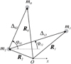Fig. 1 Schematic of the 3BP from an inertial frame (O-frame) and from a m2 -relative frame.

2 Creep Tide Model for a Circumbinary Planet

As we mention in the introduction, in the CB problem the central stars are not expected to be affected much by the planetary tidal force and, instead, are expected to evolve by mutual tides following the 2BP (e.g., Hut 1981). For this reason, we focus on the tidal evolution of the CB planet, which is expected to have a peculiar evolution due to the presence of a central binary instead of a single star.

To meet this goal we consider an extended CB planet with mass m₂ and mean radius R₂ perturbed by the tidal forces of a central binary with mass components m₀ and mi and respective radii R₀ and R₁. We assume that all the bodies share the same orbital plane and all have spin vectors perpendicular to it. From an arbitrary inertial frame, we denote by R_i the position vectors of the body m_i (i = 0, 1, 2), by Δ_j2 = R_j − R₂ (j = 0, 1) the distance from the star m_j to the planet, and by φ_j2 the angle subtended between the position of m_j and the reference axis, measured from the planet (see Fig. 1).

Then, to study the orbital dynamics of the CB planet m₂ under the effects of the tidal perturbations of each stellar component, we employ the creep theory (Ferraz-Mello 2013, 2015a) in its closed form (Folonier et al. 2018), but extended to the case of three interacting masses. In what follows, we revisit the main steps in building the 3BP extension and refer to Z2021 for details.

2.1 Revisiting the Equilibrium and Real Figure in the 3BP

To compute all the tidal forces applied on the planet, in the framework of the creep theory it is first necessary to know the real shape of the bodies. In this work we consider that the real shape of each body m_i is the result of the tidal interactions with its two partners, in addition to the polar flattening due to its rotation. Moreover, we assume that the resulting deformation is small enough to be accurately modeled up to the first order in the flattenings.

In the ideal case where each mass m_i of the 3BP is a perfectly elastic fluid that instantly responds to any external stress, it immediately adopts an equivalent equilibrium figure whose surface equation ρ_i can be approximated by a triaxial ellipsoid (Eq. (3) in Z2021), and whose flattenings and orientation can be obtained in terms of the two-body shape parameters (Eq. (4) in Z2021).

However, in a more realistic case each body is expected to have a certain viscosity that does not allow it to attain the equilibrium figure instantly. Thus, the real shape of m_; measured by the surface distance ζ_i can also be modeled by a triaxial ellipsoid, but now characterized by equatorial flattening ${\mathcal{E}}_i^{\rho }$ and polar flattening ${\mathcal{E}}_i^z$, which are a priori unknown quantities. In addition, the orientation of this real figure is also unknown but expected to lag with respect to the equilibrium orientation by an angle δ_i. The explicit surface equation of the real ellipsoid is given in Eq. (5) in Z2021.

In this model the values of $({\mathcal{E}}_i^{\rho },{\mathcal{E}}_i^z,{\delta }_i)$ are calculated at any instant of time by solving the creep equation

$${\xi }_i+{\gamma }_i{\xi }_i={\gamma }_i{\rho }_i,$$(1)

where γ_i is the relaxation factor of m_i, the only parameter of the model that is assumed to be constant in this work, and that is explicitly given by Ferraz-Mello (2013) as

$${\gamma }_i=\frac{G{d}_i{ℛ}_i}{2{\eta }_i},$$(2)

where d_i is the density, R_i the radius, and η_i the viscosity of the body, and g is the gravitational constant.

A set of three differential equations for the shape and orientation of the real figure of each body m_i is obtained by applying the creep Eq. (1). A fourth differential equation is obtained for each spin evolution Ω_i from the decoupled conservation of the total angular momentum. Then, the rotational evolution of each body m; is characterized by the differential equation set given by Eqs. (7)and(14)in Z2021.

2.2 Tidal Forces on the Planet

In Zoppetti et al. (2019a, 2020), we used the CTL model and found that for Kepler-like CB systems the characteristic tidal timescales of the planetary rotational evolution are typically much lower than those associated with the orbital evolution. Thus, CB planets are expected to have a significant orbital evolution only after reaching rotational stationary states. Then, at any instant of time the rotational state of each body m; characterized by $({\Omega }_i,{\delta }_i,{\mathcal{E}}_i^{\rho },{\mathcal{E}}_i^z)$ can be calculated by solving a differential equation system assuming fixed orbital elements (with the exception of the fast angles). Finally, the subsequent orbital evolution is expected to occur with these fixed rotational parameters.

The tidal force applied to m_j due to the deformation of m_i is given by (Z2021)

$$\begin{array}{rr}\hfill F_{ji}& \hfill =\frac{3G{m}_j{m}_i{ℛ}_i^2}{5{\Delta }_{ji}^5}[{\epsilon }_i^{\rho }\sin \left(2\left({\phi }_i^{eq}+{\delta }_i\right)-2{\phi }_{ji}\right)\left(\widehat{k}\times {\Delta }_{ji}\right)\\ \hfill & \hfill -\left(\frac{3}{2}{\epsilon }_i^{\rho }\cos \left(2\left({\phi }_i^{eq}+{\delta }_i\right)-2{\phi }_{ji}\right)+{\epsilon }_i^z\right){\Delta }_{ji}]\end{array}$$(3)

where is the orientation of the equilibrium bulge on m_; and $\widehat{k}$ is the unit vector parallel to the spin vectors.

In particular, the total tidal forces applied to planet F₂ is the result of the sum of the action forces due to the deformation on m₀ and m₁ (i.e., F₀₂ and F₁₂, respectively) plus the reaction forces that the planet exerts on each star due to its own deformation (i.e., F₂₀ and F₂₁). Thus, we have

$$F_2=\underset{\text{action\hspace{0.17em}forces}}{\underbrace{\left(F_{20}+F_{21}\right)}}+\underset{\text{reaction\hspace{0.17em}forces}}{\underbrace{\left(-F_{02}-F_{12}\right)}}.$$(4)

By comparing the amplitudes of the tidal forces in Eq. (4), it is possible to show that in standard scenarios (i.e., main sequence stars and planets with masses and radii similar to those observed in the Solar System) the stellar tides are typically much smaller with respect to the planetary tides. We note that it could happen that the tides are strong enough to lead the planet to its endpoint of tidal evolution (stationary rotational state and circular orbit) where the planetary tides become null, and the stellar tides are the only source of dissipation (e.g., Ferraz-Mello et al. 2008; Benitez-Llambay et al. 2011). However, in the general CB the presence of a secondary star always induces a non-zero mean eccentricity (e.g., Zoppetti et al. 2021b), which inhibits the CB planet from reaching the final tidal state.

As a result, tidal forces due to the deformation of the stars can typically be neglected, and only the planet needs to be considered an extended body. In this approximation the total forces on the planet can be approximated as

$$F_2\simeq -\left(F_{02}+F_{12}\right).$$(5)

We note from Eq. (5) that to compute the tidal force applied to the planet (and thus its orbital evolution), only its own rotational state needs to be known.

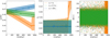Fig. 2 Tidal evolution of the Jacobian semimajor axis (leftpanel), the eccentricity (center panel), and the difference of pericenters (right panel), for a pseudo-synchronous CB planet due to creep tides. Different relaxation factors γ2 are considered with different colors (see legend in center panel). The thick curves correspond to the low-pass filtered evolution.

3 Numerical Simulations

As we mention above, the expected different orders of tidal evolution timescales allow us to assume that the orbital evolution of the planet takes place with its spin in the stationary state. In addition, in Z2021 we performed numerical simulations of the rotational evolution of a CB planet with the creep theory, and showed that the most probable stationary solution is the pseudo-synchronous state, at least for low-eccentricity planets with relaxation factors in the range estimated for the Solar System planets (e.g., Ferraz-Mello 2013).

The mean values around which the pseudo-synchronous rotational solution oscillates were presented in Eq. (16)–(19) in Z2021. The oscillation amplitudes of this solution were discussed in Zoppetti et al. (2021b). In Appendix A we discuss an accurate approximation of these amplitudes and provide the explicit set of coefficients employed in this work to characterize the oscillations around the pseudo-synchronous state.

With these two motivations, in what follows we study the orbital evolution of a CB planet whose rotational evolution has reached the pseudo-synchronous state. As initial conditions of our numerical simulations, we chose a Kepler-38-type system (Orosz et al. 2012a), which has been the working example of several of our previous works (e.g., Zoppetti et al. 2018, 2019a, 2021a). The nominal values for the system parameters and initial orbital elements are detailed in Table 1. The body masses and radii were taken close to the observed values, with two exceptions: the primary radius R₀ corresponds to an estimation obtained from backward star evolutionary tracks (Zoppetti et al. 2018), while the mass m₂ was estimated from a semi-empirical mass-radius fit following Mills & Mazeh (2017).

Figure 2 shows the orbital evolution of a CB planet with initial conditions given in Table 1. To perform the simulation we integrate the gravitational 3BP, but also consider that the planet undergoes a tidal force given by Eq. (5). The rotational state of the CB planet is analytically set in the pseudo-synchronous solution in the whole numerical integration. We explore different rheologies for the planet by considering three different relaxation factors: γ₂/n₂ = 10 in blue (representing a planet in what we call the gaseous regime), γ₂/n₂ = 0.1 in green (representing a planet in the stiff regime) and γ₂/n₂ = 1 in orange (representing a planet in transition). The planetary semimajor axis a₂ evolution is shown in the left panel, the eccentricity evolution e₂ in the center panel, and the difference of pericentre longitudes Δϖ = ϖ₁ − ϖ₂ in the right panel. The results after the application of the low-pass filter are shown as darker curves for a₂ and e₂.

For the considered initial conditions, perhaps the most interesting feature that can be observed in Fig. 2 is that the tidal migration direction depends on the planetary relaxation factor; for pseudo-synchronized planets with γ₂/n₂ = 10 the migration in semimajor axis is outward, while the direction of migration of planets with γ₂/n₂ = 0.1 is inward. Although not shown in Fig. 2, the outward migration is observed for any planet with γ₂ ≫ n₂, while inward migration is always obtained for the case γ₂ ≪ n₂. However, we note that the characteristic timescales for the semimajor axis evolution predicted by our numerical simulations are very long, about two orders of magnitude longer than the estimated lifetime of the Kepler-38 system (Orosz et al. 2012a).

In particular, observing the orange curves in all the panels of Fig. 2 we note that the orbital elements abruptly change their evolution at ~900 Gyr. This is due to the CB planet (which was initially with n₁/n₂ ~ 5.6) having such a migration in the semi-major axis that finishes its evolution captured in the 5:1 mean motion resonance, with the consequent excitation in eccentricity and circulation of the difference of pericenters. We recall from the tidal 2BP results (e.g., Folonier et al. 2018) that the case γ₂/n₂ = 1 represents the situation in which the dissipation of energy is at its maximum, which translates into maximum orbital evolution, a phenomenon that we also observe in our problem (compare color curves in left panel of Fig. 2).

On the other hand, in Fig. 2 we observe that the eccentricity and the pericenter evolution seem to be little affected by the tides, and instead are dominated by the purely gravitational dynamics of the 3BP. The CB planetary eccentricity oscillates around a mean eccentricity 〈e₂〉, which is a combination of the forced eccentricity (Moriwaki & Nakagawa 2004) and the semi-mean eccentricity (Paardekooper et al. 2012; see Zoppetti et al. 2019b for details). Then the smooth (increasing or decreasing) secular evolution observed is an indirect consequence of the semiaxis migration; since 〈e₂〉 is inversely proportional to a₂, when the planet migrates outward the mean eccentricity decrease, while the opposite occurs when the planet migrates inward.

In the right panel of Fig. 2 we note, independently of the relaxation factors considered, that the difference of pericenter longitudes Δϖ shows a libration of high amplitude around ~0°, which corresponds to the Mode 0 secular mode (Michtchenko & Malhotra 2004). As we noted in Zoppetti et al. (2019a), this angle coupling should be taken into account when constructing models averaged in the pericenters, which usually assume that m₁ and m₂ vary independently.

We finally mention that due to the extremely long timescales of orbital tidal evolution (see timescales on the x-axis of panels in Fig. 2), we needed to employ a numerical technique in order to obtain reasonable computational integration times. With this aim, we artificially introduced an acceleration factor Γ in the tidal forces of Eq. (5) to scale down the time span of the numerical integration. We were careful to consider only small values of Γ in order for the tidal force to remain adiabatic with respect to the pure gravitational interaction. In addition, we also checked for short time intervals to obtain an identical evolution with respect to the non-accelerated simulation. However, the data output had to be strongly limited, and it seems not to have been large enough to result in a soft filtration (see thick curves in left and center panels of Fig. 2).

4 Analytical Model for the Secular Orbital Evolution

To understand the problem in greater depth and to better explain the results of the numerical simulations, we constructed an analytical secular model for the orbital evolution of a CB planet in the pseudo-synchronous rotational state.

With this goal, we first adopted the Jacobian reference frame in which the state vector of the secondary star is m₀ -centric, but the planetary state vector is calculated from the barycenter of the binary. Then we again considered that the CB planet is the only extended mass in the system, and is locked in the pseudo-synchronous state described by the mean values given in Eqs. (16)–(19) in Z2021, and the oscillation amplitudes given in Appendix A.

4.1 Orbital Evolution of CB Planets

In the Jacobian frame, the variational equation for the planetary semimajor axis a₂ can be written as (e.g., Beutler 2005)

$$\frac{\text{d}{a}_2}{\text{d}t}=\frac{2a_2^2}{\mathcal{G}\left(m_0+m_1+m_2\right)}\left({\dot{\rho }}_2\cdot \delta f_2\right),$$(6)

where δf₂ is the total tidal force per unit mass perturbing the two-body motion of the planet around the center of mass of the binary. It is explicitly related to the total tidal force by means of the reduced mass ${\beta }_2=\frac{(m_0+m_1)m_1}{(m_0+m_1+m_2)}$ as (e.g., Zoppetti et al. 2019a)

$$\delta f_2=\frac{1}{{\beta }_2}{F}_2.$$(7)

By substituting the total tidal force in Eq. (5) into Eq. (6); expanding in power series of α = α₁ /α₂, e₁, and e₂; and finally averaging over the mean longitudes, we obtain

$$\langle \frac{\text{d}{a}_2}{\text{d}t}\rangle =\frac{n_2\left(m_0+m_1\right){ℛ}_2^5}{m_2{a}_2^4}{\displaystyle \sum _{i=0}^4{A}_i^{\left(a\right)}}{\alpha }^i,$$(8)

which is developed up to the fourth order in α and up to the second order in the eccentricities, with the exception of the α⁴- term which is up to the zeroth order in these small parameters. The non-null coefficients are

$$\begin{array}{r}\hfill A_0^{\left(a\right)}=-\frac{63}{2}\frac{{\gamma }_2{n}_2}{{\gamma }_2^2+n_2^2}{e}_2^2,\\ \hfill A_2^{\left(a\right)}=-\frac{225}{2}{ℳ}_2\frac{{\gamma }_2{n}_2}{{\gamma }_2^2+n_2^2}{e}_2^2,\\ \hfill A_3^{\left(a\right)}=\frac{225}{2}{ℳ}_3\frac{{\gamma }_2{n}_2}{{\gamma }_2^2+n_2^2}{e}_1{e}_2\cos \left(\Delta \overline{\omega }\right),\\ \hfill A_2^{\left(a\right)}=\frac{1557}{16}{ℳ}_2^2\frac{{\gamma }_2\left(2n_1-2n_2\right)}{{\gamma }_2^2+{\left(2n_1-2n_2\right)}^2},\end{array}$$(9)

with

$${ℳ}_2=\frac{m_0{m}_1}{{\left(m_0+m_1\right)}^2};{ℳ}_3=\frac{m_0{m}_1\left(m_0-m_1\right)}{{\left(m_0+m_1\right)}^3}.$$

As we mention in Sect. 3, unlike the semimajor axis case, the presence of a massive secondary star companion induces a mean eccentricity 〈e₂〉 in the planet that is the main secular attractor on secular timescales. Thus, in the CB context, the expected effect of the tidal forces on this orbital element is that it will lead to the equilibrium gravitational solution by damping the free eccentricity, which depends on the initial conditions. However, to understand the dependence of this damping on the physical and orbital parameters of the system, we also compute the secular tidal evolution of the CB eccentricity, but only up to low order in α.

This variational equation can be obtained by differentiating the planetary orbital angular momentum $L_2={\beta }_2\sqrt{\mathcal{G}(m_0+m_1+m_2)a_2(1-e_2^2)}$ as (e.g., Zoppetti et al. 2019a)

$$\frac{\text{d}\left(e_2^2\right)}{\text{d}t}=\frac{1}{a_2}\left[\left(1-e_2^2\right)\frac{\text{d}{a}_2}{\text{d}t}-\frac{2L_2}{\mathcal{G}\left(m_0+m_1\right)m_2}\left(\left({\rho }_2\times \delta f_2\right)\cdot \widehat{k}\right)\right],$$(10)

and then proceeding in the same manner as for obtaining Eq. (8). Up to second order in α and the eccentricities, we have

$$\langle \frac{\text{d}{e}_2^2}{\text{d}t}\rangle =-\frac{n_2\left(m_0+m_1\right){ℛ}_2^5}{m_2{a}_2^5}\frac{{\gamma }_2{n}_2}{{\gamma }_2^2+n_2^2}\left(\frac{63}{2}+\frac{225}{2}{ℳ}_2{\alpha }^2\right)e_2^2.$$(11)

In Fig. 3 we show the secular planetary semimajor axis (left panels) and eccentricity evolution (right panels) obtained with our model for a pseudo-synchronous CB planet as a function of its normalized relaxation factor. We consider different values of the semimajor axis ratio: α = α_K38 ≃ 0.32 (see Table 1) in the upper panels and α = 0.5α_K38 = 0.16 in the lower panels. Different types of curves represent different methods for computing the temporal evolution: numerical averaging (solid curves) and analytical approximation (Eqs. (8) and (11)) (dashed curves). The different colors represent different planetary eccentricity values, as indicated in the upper left panel.

Regarding the pure effect of creep tides on the planetary eccentricity (right panels of Fig. 3), we observe similar results to those predicted by the 2BP: tides always cause an eccentricity damping that is strongly proportional to the proximity to the disturber and also to the eccentricity of the perturbed body. This can also be seen from the analytical Eq. (11), where the zeroth order (i.e., the 2BP coefficient) is at least two orders of magnitude larger than the second-order term (i.e., the 3BP term). However, one of the main differences between tides on a CB planet with respect to tides on a planet around a single star is that in the former case eccentricity is not able to be damped to zero due to the non-zero mean eccentricity 〈e₂〉 induced by the presence of a secondary star.

According to our model, the tidal secular evolution in the semimajor axis of pseudo-synchronous CB planets is much richer, especially in regions close to the binary where the confirmed CB systems are located (see upper left panel of Fig. 3). On the one hand, for CB planets in the stiff regime the direction of migration is always inward and more important for eccentric planets. On the other hand, for planets in the gaseous regime the direction of migration is the result of a competition between the planetary eccentricity and the proximity to the binary; eccentric and wide CB planets tend to migrate inward (as the scenario resembles the 2BP), while low-eccentricity and tight CB planets tend to migrate outward. This last result for the gaseous regime was reported in our previous work by using the CTL model Zoppetti et al. (2019a, 2020).

Regarding the accuracy of our model, a simple comparison of the different type of curves of Fig. 3 shows that the analytical approximation represent a very good fit of the numerical simulation. However, strictly speaking γ₂ is not a small parameter of our model. Then, in Fig. 4 we consider two particular γ₂-values and validate our analytical approach of the planetary semimajor axis tidal evolution as a function of α. We employ the same convention for the type of curves and colors as that used in Fig. 3.

We note in Fig. 4 that for low-eccentricity CB planets this approximation represents a very good fit of the numerical behavior, even for high α-values such as those observed in the confirmed CB population. The accuracy of the analytical fit does not seem to be strongly dependent on the viscosity regime, but becomes less precise for eccentric planets because e₂ is another small parameter of the model. Although it is not explored in Fig. 4, we observe only a smooth dependence of the results with the binary eccentricity e₁, which seems to be a parameter of secondary importance in determining the semimajor axis secular evolution due to tides. This is consistent with the analytical expectation, since the dependence with e1 only appears up to the third order in α (see Eq. (8)).

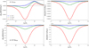Fig. 3 Secular orbital evolution of the semimajor axis (left panels) and eccentricity (right panels) of a pseudo-synchronous CB planet due to creep tides, as a function of its normalized relaxation factor. The solid curves are the results of a numerical averaging of the full evolution equations, while the dashed curves represent the results of our analytical secular model. Different α-values are used in the different rows and different planetary eccentricities are shown in the different colors. The region γ2/n2 > 1 approximately corresponds to the gaseous regime while the region γ2/n2 < 1 corresponds to the stiff regime.

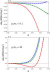Fig. 4 Secular semimajor axis evolution of a pseudo-synchronous CB planet due to creep tides, as a function of its distance to the binary measured with α = a1/a2. In the different panels CB planets in different viscosity regimes are considered. The different types of curves and different colors are the same as those for Fig. 3.

4.2 Application to Kepler Systems

In the previous subsection we confirm with a secular analytical model the results obtained in Sect. 3 with numerical simulations that the direction of tidal migration of pseudo-synchronous CB planets depends not only on the physical parameters of the system and orbital elements, but also (and curiously) on the viscosity regime of the planet. This makes the tidal orbital evolution of CB planets much more complex compared to the 2BP case, and prevents us from establishing the general migration trends of the systems (and thus the general evolution histories), without knowing the particular characteristics of the physical parameters.

In Table 2 we consider the sample of confirmed CB planets, where with only one exception (i.e., TOI-1338) all the systems were discovered by the Kepler mission. We use the estimated α = a₁/a₂, e₂, and M₂ according to the discovery papers unless otherwise stated. We estimate its viscosity regime by considering its observed mass, then inferring its γ₂-values by comparison with the Solar System planet estimations of Ferraz-Mello (2013), and finally compared with the fundamental frequencies of the system n₁ and n₂. We note that probably due to an observational bias the discovered CB planets are typical of high radius (and high mass), so their relaxation factors γ₂ are expected to be similar to those of Neptune or Saturn, then much higher than the fundamental frequencies of the system, and thus are expected to be in the gaseous regime. For the case of Kepler-38 and Kepler-47c, the estimated range of planetary mass is too large to estimate a reliable viscosity regime.

To explore its evolutionary history due to tides, we note that for close CB planets where tidal forces are expected to play an important role (i.e., discarding Kepler-47d, Kepler-47c, and Kepler-1647), the mean semimajor axis ratio is 〈α₂〈 ≃ 0.28 and the mean planetary eccentricity is 〈e₂〉 ≃ 0.07. Thus, we have that 〈α〉² ~ 〈e₂〉, and the analytical tidal semimajor axis evolution given in Eq. (8) is expected to be governed by only the α⁰ term with coefficient $A_0^{(a)}$ plus the α⁴ term with coefficient $A_4^{(a)}$.

4.2.1 Direction of Tidal Migration

Using this approach, the change in the migration direction that occurs when $\langle \frac{\text{d}{a}_2}{\text{d}t}\rangle =0$ implies

$$A_0^{\left(a\right)}+A_4^{\left(a\right)}{\alpha }_{\text{crit}}^4=0,$$(12)

where the semimajor axis ratio α_crit represents the critical value such that systems in which α > α_cгit CB planets migrate outward (i.e., $\langle \frac{\text{d}{a}_2}{\text{d}t}\rangle >0$), while in those systems where α < α_cгit the planets experience an inward secular tidal evolution (i.e., $\langle \frac{\text{d}{a}_2}{\text{d}t}\rangle <0$) according to our analytical model. Its explicit expression is

$${\alpha }_{\text{crit}}^4=\frac{28}{173}\frac{n_2}{n_1-n_2}\left(\frac{{\gamma }_2^2+{\left(2n_1-2n_2\right)}^2}{{\gamma }_2^2+n_2^2}\right)\frac{e_2^2}{{ℳ}_2^2}.$$(13)

We note that this equation contains some of the results previously reported. First, in the limit m₁ → 0, M₂ → 0, and α_cгit → ∞. Then, when α < ∞ the predicted migration direction is always inward, as is well known in the 2BP for pseudo-synchronous bodies. Second, in the limit of circular planetary orbit e₂ → 0, α_cгit → 0. Then, when α > 0 in all the cases the direction of migration is always outward, as we previously reported with the CTL model (e.g., Zoppetti et al. 2019a, 2020).

Thus, if we assume that the confirmed CB planet has acquired its pseudo-synchronous rotational solution, Eq. ( 3) allows us to estimate the direction of tidal migration through computing α_cгit, which only depends on parameters that can be derived from classical transit observations, except the relaxation factor γ₂. However, this dependence can be avoided if we can somehow infer the viscosity regime, for example using mass estimations and comparison with Solar System planet parameters.

For CB planets in the gaseous regime, we expect γ₂ ≫ n₁, n₂ and then Eq. ( 3) becomes

$${\alpha }_{\text{crit,g}}^4=\frac{28}{173}\frac{n_2}{n_1-n_2}\frac{e_2^2}{{ℳ}_2^2}.$$(14)

For the particular case of Kepler-38 (see Table 1) we have α_crit,g ≃ 0.16. Then, if we assume that the CB planet is in this regime, because α_K38 > α_crit,g our model predicts an outward migration, in agreement with what we previously reported in Zoppetti et al. (2018, 2019a, 2020). Moreover, this analytical estimation is consistent with the outward migration observed in the left panel of Fig. 2 for the case γ₂ = 10n₂ (blue curve).

On the other hand, for CB planets in the stiff regime we have γ₂ ≪ n₁, n₂ and the critical semimajor axis of Eq. (13) is now simply given by

$${\alpha }_{\text{crit,s}}^4=\frac{112}{173}\frac{n_1-n_2}{n_2}\frac{e_2^2}{{ℳ}_2^2}.$$(15)

Again, for the case of Kepler-38 we have α_crit,s = 0.49. Then, if the CB planet is assumed to be a stiff body α_K38 < α_crit,s, our model predicts an inward migration. We note that this is exactly what we observe in the left panel of Fig. 2 for the case γ₂ = 0.1n₂ (green curve).

In Table 2, we also compute for each confirmed CB system the parameters α_crit,g and α_crit,s, following Eqs. (14) and (15), respectively. We highlight the parameter (in bold) that has to be specially considered due to the estimation of the viscosity regime. By comparing the α-value of the planet with the critical values, we infer the direction of tidal migration in the semimajor axis. As can be seen in Table 2, these directions strongly depend on the particular parameters of the system, especially on the distance to the binary and the planetary eccentricity. In particular, the planet Kepler-47c is so far from the binary that our model predicts an inward migration, regardless of its particular viscosity.

We finally note that the parameter α_crit in Eq. (13) can also be interpreted as a quantification of the tidal interaction that dominates the migration of the CB planet. If α_crit < 0, then $\left|A_4^{(a)}\right|<\left|A_0^{(a)}\right|$, and the tidal evolution is mainly governed by the classical 2BP, where n2 is the main dynamical frequency; in the opposite case, $\left|A_4^{(a)}\right|>\left|A_0^{(a)}\right|$ and the tides are dominated by the 3BP with a central dipole, whose fundamental frequency is 2n₁ − 2n₂. Thus, in the case of inward migrating planets the maximum possible tidal energy dissipated can be estimated by setting γ₂ = n₂, while for outward migrating CB planets it can be estimated with γ₂ = 2n₁ − 2n₂.

4.2.2 Orbital Evolution Timescales

We now use our simplified analytical model to estimate the timescales of semimajor axis evolution due to creep tides, using the observed physical parameters and the current values of α and e₂ given in Table 2.

Using the approach described in Sect. 4.2.1, the tidal timescales in the semimajor axis can be estimated as

$$\begin{array}{rr}\hfill {\tau }_a& \hfill =\frac{a_2}{\langle \frac{\text{d}{a}_2}{\text{d}t}\rangle }\\ \hfill & \hfill \simeq \frac{1}{n_2}{\left(\frac{a_2}{{ℛ}_2}\right)}^2\left(\frac{m_2}{m_0+m_1}\right)\frac{1}{\left|-\frac{63}{2}\frac{{\gamma }_2{n}_2}{{\gamma }_2^2+n_2^2}{e}_2^2+\frac{1557}{16}{ℳ}_2^2\frac{{\gamma }_2\left(2n_1-2n_2\right)}{{\gamma }_2^2+\left(2n_1-2n_2\right)}{\alpha }^4\right|}\end{array}.$$(16)

In the regime of gaseous bodies, the limit case of minimum tidal timescales (i.e., maximum semimajor axis variation) occurs for γ₂ = 2n₁ − 2n₂, and the timescale is

$${\tau }_{\text{a,gas}}^{\min }\simeq \frac{1}{n_2}{\left(\frac{a_2}{{ℛ}_2}\right)}^5\left(\frac{m_2}{m_0+m_1}\right)\frac{1}{\left|-\frac{64}{4}\frac{n_2}{n_1-n_2}{e}_2^2+\frac{1557}{16}{ℳ}_2^2{\alpha }^4\right|}.$$(17)

Analogously, in the regime of stiff bodies the limit case of minimum timescales of semimajor axis evolution occurs for γ₂ = n₂ and is given by

$${\tau }_{\text{a,sti}}^{\min }\simeq \frac{1}{n_2}{\left(\frac{a_2}{{ℛ}_2}\right)}^5\left(\frac{m_2}{m_0+m_1}\right)\frac{1}{\left|-\frac{63}{2}{e}_2^2+\frac{1557}{32}{ℳ}_2^2\frac{n_2}{n_1-n_2}{\alpha }^4\right|}.$$(18)

These minimum timescale estimations for the semimajor axis evolution (Eqs. (16) and (17)) are also included in Table 2 for each specific system. As can be observed, independently of the viscosity regime in which the CB planet is assumed to be, the tidal timescales for semimajor axis evolution are at least three orders of magnitude greater than the age of the system. Then, according to our model, the observed sample of discovered CB planets are not expected to have had a relevant semimajor axis migration.

4.2.3 The CTL Limit

Following Ferraz-Mello (2013) (see Sect. 7.1), we can relate the planetary relaxation factor y₂ with the classical dissipation factor Q₂, and from this with the lag angle ϵ₂ = 1/Q₂. Unlike the constant phase lag model (e.g., MacDonald 1964), in the creep tide theory this quantity is not constant, but depends on the tidal frequency ν as

$$Q_2\left(v\right)=\frac{1}{{ϵ}_2\left(v\right)}=\frac{2}{3}{k}_{2,2}\frac{{\gamma }_2^2+v^2}{{\gamma }_{2}v},$$(19)

where k_2,2 is the planetary tidal Love number, and we consider a homogeneous sphere planetary fluid Love number (i.e., k_f2 = 1.5).

In the CTL model (e.g., Mignard 1979), the phase lag is assumed to be proportional to the tidal frequency ϵ(ν) = ν∆t₂, where the proportionality factor ∆t₂ represents the time lag of the tidal bulge, and is assumed to be constant and equal for all the tidal frequencies in the model. Thus, the link between the two model parameters is given by

$$k_{2,2}\Delta t_2=\frac{3}{2}\frac{{\gamma }_2}{{\gamma }_2^2+v^2}.$$(20)

Using the relation given in Eq. (20) in the computation of the coefficients that characterize the secular tidal evolution with the creep theory (Eqs. (9) and (11)), we obtain the same coefficients as those obtained with the pure CTL model detailed in the next section.

5 Revisiting the Orbital Evolution of a CB Planet in the CTL Model

5.1 CTL Tidal Forces Including Cross Tides

Similarly to what we find in Z2021 for the case of the rotational evolution, the orbital evolution of synchronous bodies that results from Eqs. (8) and (10) in the case of gaseous bodies (i.e., γ₂ ≫ n₂) does not fit with the evolution calculated in Zoppetti et al. (2019a) with the CTL model. The reason for this discrepancy is that in our previous work the cross tides were neglected. In what follows we build a CTL model for the CB problem that includes the cross tidal forces, and show that it predicts a secular orbital evolution for the planet that is identical to that predicted by the creep model in the limit of gaseous bodies.

With this goal we again consider the 3BP composed of m₀, m₁, and m₂, where all the tidal interactions between pairs are taken into account. Then, due to the presence of each body m_i, one ellipsoid is generated on m_i and one ellipsoid on m_k. Here we denote as $F_{i,j}^k$ the tidal force applied to m_i due to the ellipsoid that the presence of m_k generates on m_j (see Sect. 5 of Z2021 for details). For the particular case of a CB planet m₂, we have

$$F_2=\underset{\text{direct tides}}{\underbrace{\left(F_{2,0}^2+F_{2,1}^2-F_{0,2}^0-F_{1,2}^1\right)}}+\underset{\text{cross tides}}{\underbrace{\left(F_{2,0}^1+F_{2,1}^0-F_{0,2}^1-F_{1,2}^0\right)}}$$(21)

We recall that the forces with three different indexes in Eq. (21) correspond to the cross tides (which were neglected in Zoppetti et al. 2019a), while the forces with two repeated indexes correspond to the direct tides (which we did consider in the same work). We also note that the CTL force Eq. (21) is very similar to the creep force Eq. (4); the only difference is that in the Newtonian creep formalism we work with the equivalent ellipsoid that results from the sum of the ellipsoids generated by the pairwise interactions. In the classical CTL model of Mignard (1979), the interacting tidal force $F_{i,j}^k$. is expanded up to first order in the time lag ∆t_j as

$$F_{i,j}^k=F_{i,j}^{k,\left(0\right)}+\Delta t_j{F}_{i,j}^{k,\left(1\right)},$$(22)

where the explicit expressions of $F_{i,j}^{k,(0)}$ and $F_{i,j}^{k,(1)}$ are respectively given in Eqs. (25) and (26) in Z2021.

5.2 Orbital Evolution of the Full Problem

Using Eqs. (5) and (6), but now with the Mignard force given in Eq. (21), the secular variation of the planetary semimajor axis expanded up to fourth order in α and up to second order in the eccentricities is given by

$$\langle \frac{\text{d}{a}_2}{\text{d}t}\rangle =\frac{n_2}{\mathcal{G}ℳa_2^4}{\displaystyle \sum _{i=0}^4{\displaystyle \sum _{i,j=0}^2{A}_{i,jk}^{\left(a\right)}{\alpha }^i{e}_1^j{e}_2^k}},$$(23)

where

$$\begin{array}{lll}{A}_{0,0,0}^{\left(a\right)}\hfill & =\hfill & K_2\left(2{\Omega }_2-2n_2\right)+{ℳ}^2{\displaystyle \sum _{i=0}^1{K}_i\left(2{\Omega }_i-2n_2\right)},\hfill \\ A_{0,0,2}^{\left(a\right)}\hfill & =\hfill & K_2\left(27{\Omega }_2-46n_2\right)+{ℳ}^2{\displaystyle \sum _{i=0}^1{K}_i\left(27{\Omega }_i-46n_2\right)},\hfill \\ A_{1,1,1}^{\left(a\right)}\hfill & =\hfill & 6{ℳ}^2{\displaystyle \sum _{i=0}^1{K}_i{\beta }_i\left(12{\Omega }_i-19n_2\right)\cos \Delta \overline{\omega },}\hfill \\ A_{2,0,0}^{\left(a\right)}\hfill & =\hfill & 5{ℳ}_2{K}_2\left({\Omega }_2-n_2\right)\hfill \\ \hfill & \hfill & +{ℳ}^2{\displaystyle \sum _{i=0}^1{K}_i{\beta }_i^2\left(24{\Omega }_i+10n_1-34n_2\right),}\hfill \\ A_{2,2,0}^{\left(a\right)}\hfill & =\hfill & \frac{15}{2}{ℳ}_2{K}_2\left({\Omega }_2-n_2\right)\hfill \\ \hfill & \hfill & +{ℳ}^2{\displaystyle \sum _{i=0}^1{K}_i{\beta }_i^2\left(36{\Omega }_i-5n_1-51n_2\right),}\hfill \\ A_{2,0,2}^{\left(a\right)}\hfill & =\hfill & 5{ℳ}_2{K}_2\left(22{\Omega }_2-35n_2\right)\hfill \\ \hfill & \hfill & +{ℳ}^2{\displaystyle \sum _{i=0}^1{K}_i{\beta }_i^2\left(528{\Omega }_i+220n_1-1135n_2\right),}\hfill \\ A_{3,1,1}^{\left(a\right)}\hfill & =\hfill & (-\frac{75}{8}{ℳ}_3{K}_2\left(16{\Omega }_2-23n_2\right)\hfill \\ \hfill & \hfill & +\frac{25}{2}{ℳ}^2{\displaystyle \sum _{i=0}^1{K}_i{\beta }_i^3\left(96{\Omega }_i+32n_1-193n_2\right)})\cos \Delta \overline{\omega },\hfill \\ A_{4,0,0}^{\left(a\right)}\hfill & =\hfill & \frac{5}{16}{ℳ}_2^2{K}_2[21\frac{\left(m_0^2+m_1^2\right)}{m_0{m}_1}\left({\Omega }_2-n_2\right)\hfill \\ \hfill & \hfill & +26\left(9{\Omega }_2+10n_1-19n_2\right)]\hfill \\ \hfill & \hfill & 20{ℳ}^2{\displaystyle \sum _{i=0}^1{K}_i{\beta }_i^4\left(6{\Omega }_i+5n_1-11n_2\right),}\hfill \\ A_{4,2,0}^{\left(a\right)}\hfill & =\hfill & \frac{25}{16}{ℳ}_2^2{K}_2[21\frac{\left(m_0^2+m_1^2\right)}{m_0{m}_1}\left({\Omega }_2-n_2\right)\hfill \\ \hfill & \hfill & +26\left(9{\Omega }_2+2n_1-19n_2\right)]\hfill \\ \hfill & \hfill & +100{ℳ}^2{\displaystyle \sum _{i=0}^1{K}_i{\beta }_i^4\left(6{\Omega }_i+n_1-11n_2\right),}\hfill \\ A_{4,0,2}^{\left(a\right)}\hfill & =\hfill & \frac{5}{32}{ℳ}_2^2{K}_2[21\frac{\left(m_0^2+m_1^2\right)}{m_0{m}_1}\left(65{\Omega }_2-98n_2\right)\hfill \\ \hfill & \hfill & +26\left(585{\Omega }_2+650n_1-1722n_2\right)]\hfill \\ \hfill & \hfill & +10{ℳ}^2{\displaystyle \sum _{i=0}^1{K}_i{\beta }_i^4\left(390{\Omega }_i+325n_1-1008n_2\right),}\hfill \end{array}$$(24)

where $K_i=3\mathcal{G}{\mathcal{R}}_i^5{k}_{2i}\Delta t_i,\mathcal{M}=\frac{m_2}{m_0+m_1}$ and

$${\beta }_0=\frac{m_1}{m_0+m_1};{\beta }_1=-\frac{m_0}{m_0+m_1}.$$(25)

The secular variation in the planetary eccentricity up to the second order in the small parameters is given by

$$\langle \frac{\text{d}{e}_2^2}{\text{d}t}\rangle =\frac{n_2}{\mathcal{G}ℳa_2^5}{\displaystyle \sum _{i=0}^2{\displaystyle \sum _{i,j=0}^2{A}_{i,j=0}^{\left(e\right)}{\alpha }^i{e}_1^j{e}_2^k,}}$$(26)

where

$$\begin{array}{lll}{A}_{0,0,2}^{\left(e\right)}\hfill & =\hfill & K_2\left(11{\Omega }_2-18n_2\right)+{ℳ}^2{\displaystyle \sum _{i=0}^1{K}_i\left(11{\Omega }_i-18n_2\right),}\hfill \\ A_{1,1,1}^{\left(e\right)}\hfill & =\hfill & \frac{1}{8}{ℳ}^2{\displaystyle \sum _{i=0}^1{K}_i{\beta }_i\left(156{\Omega }_i+5\frac{m_1{a}_2^3}{m_1{a}_1^3}{n}_1-216n_2\right)\cos \left(\Delta \overline{\omega }\right),}\hfill \\ A_{2,0,2}^{\left(e\right)}\hfill & =\hfill & \frac{25}{2}{ℳ}_2{K}_2\left(36{\Omega }_2-5n_2\right)\hfill \\ \hfill & \hfill & +5{ℳ}^2{\displaystyle \sum _{i=0}^1{K}_i{\beta }_i^2\left(36{\Omega }_i+15n_1-74n_2\right)}.\hfill \end{array}$$(27)

Equations (23) and (26) describe the orbital evolution of an extended CB body rotating with arbitrary angular velocity Ω₂, around a binary whose components are also considered as extended objects and are rotating with arbitrary spins Ω₀ and Ω₁. In the next subsection we discuss the particular case in which the system has physical and orbital parameters similar to those observed in the confirmed CB systems of Table 2.

5.3 Analytic Orbital Solution for Punctual Stars and Synchronous CB Planets

The secular planetary orbital evolution for the case in which the stars are assumed to be punctual can be easily obtained by setting K₀ = K₁ = 0 in the coefficients of Eqs. (24) and (27). In this case it is possible to see, for low-eccentricity CB planets far from the pseudo-synchronous state, that the tidal secular evolution is mainly dominated by the zeroth-order term in α, which is at least two orders of magnitude greater than the rest. Thus, according to this model CB planets in free rotation are expected to have a similar secular orbital evolution to that obtained for its analogs around single stars. In what follows we see that this is not the case for CB planets in the pseudo-synchronous stationary state.

As previously mentioned, we expect very different tidal timescales of the rotational evolution with respect to the orbital evolution. This allows us to assume that a significant orbital evolution only occurs with the planet in its pseudo-synchronous rotational steady state.

The mean value of the CB planet spin in the pseudo-synchronous solution can be estimated by Eqs. (16) in Z2021. In the limit of gaseous bodies in which the CTL model may serve as the first approximation (e.g., Efroimsky 2012, 2015), this stationary pseudo-synchronous spin expanded up to the fourth order in α and up to the second order in the eccentricities (with the exception of the α⁴) is

$$\begin{array}{lll}\langle {\Omega }_2\rangle /n_2\hfill & =\hfill & 1+\left(6+5{ℳ}_2{\alpha }^2\right)e_2^2\hfill \\ \hfill & \hfill & -\frac{325}{16}{e}_1{e}_2\cos \left(\Delta \overline{\omega }\right){ℳ}_3{\alpha }^3-19\left(\frac{n_1}{n_2}-1\right){ℳ}_2^2{\alpha }^4\hfill \end{array}.$$(28)

For this particular rotational configuration the secular semimajor axis evolution is simply given by

$$\begin{array}{lll}\langle \frac{\text{d}{a}_2}{\text{d}t}\rangle \hfill & =\hfill & \frac{3n_2^2{ℛ}_2^5{k}_{2,2}\Delta t_2}{ℳa_2^4}(-7e_2^2-25{ℳ}_2{e}_2^2{\alpha }^2\hfill \\ \hfill & \hfill & -25{ℳ}_3{e}_1{e}_2\cos \left(\Delta \overline{\omega }\right){\alpha }^3+\frac{173}{4}{ℳ}_2^2\left(\frac{n_1}{n_2}-1\right){\alpha }^4),\hfill \end{array}$$(29)

while the secular eccentricity evolution is given by

$$\langle \frac{\text{d}{e}_2^2}{\text{d}t}\rangle =-\frac{3n_2^2{ℛ}_2^5{k}_{2,2}\Delta t_2}{{ℳ}_2{a}_2^5}\left(7+25{ℳ}_2{\alpha }^2\right)e_2^2.$$(30)

It is easy to see that expressions (29) and (30) are identical to the expressions obtained in the creep tide theory, when we consider the gaseous bodies limit (see Sect. 4.2.3).

6 Summary and Discussion

In this work we presented an extension of the creep tide theory first developed in Ferraz-Mello (2013) to study the orbital evolution of a coplanar circumbinary planet without obliquity. A simple analysis of the amplitudes of the tidal forces shows, at least for CB systems like those confirmed here, that the tides on the planet that are due to the stars are much greater than the tides on the stars. Then, we studied the problem under the assumption that the stellar components are punctual masses.

In addition, in this work, we took advantage of two previously reported results for the rotation of CB planets, which considerably simplified the problem. On the one hand, the timescales of the rotational evolution of the CB planet are expected to be much smaller than the orbital evolution (Zoppetti et al. 2019a, 2020). On the other hand, for low-eccentricity CB planets with viscosities similar to the values estimated for the Solar System bodies (Ferraz-Mello 2013), the most probable final stationary rotational state is the pseudo-synchronous (Z2021). Thus, instead of solving the full differential equations system (i.e., rotation + orbit), we only solved the subsystem associated with the orbital evolution, assuming the pseudo-synchronous whose mean values are given in Z2021 and oscillation amplitudes are discussed in Zoppetti et al. (2021b) and given in Appendix A.

Assuming this rotational state, we then briefly revisited the formalism presented in Z2021 to extend the creep theory to the CB problem. As in our previous work, we used a Kepler38-type system as a working example. Although this is the reference system of our investigation, we also explored a wide range of physical parameters to obtain general results valid for a large number of CB planets (already and yet-to-be discovered).

We performed direct numerical integrations of gravitational 3BP on the planet and studied the secular orbital evolution due to the creep tides on it considering different planetary relaxation factors y2. Regarding the eccentricity and pericenter evolution, we find that in this context they are little affected by the tides, but instead are dominated by the pure 3BP gravitational interactions. In particular, as confirmed later with the analytical model and similar to the effect expected in the 2BP, tides try to circularize the orbit of CB planets. However, the presence of the secondary star induces a mean eccentricity that is even non-zero for a circular binary (e.g., Zoppetti et al. 2019b). This pure gravitational equilibrium governs the secular eccentricity of the CB planets and inhibits the perfect circularization of their orbits. Thus, the effect of tides on these orbital elements is that it simply leads to this equilibrium solution.

However, the secular evolution of the CB planetary semimajor axis shows a very curious behavior in our numerical simulations. For relaxation factors much greater than the mean motion of the planet (what we call the gaseous regime), the planet exhibits an outward migration, as was reported in our previous works with the CTL model (Zoppetti et al. 2018, 2019a). On the other hand, for relaxation factors much lower than the mean motion (what we call the stiff regime), the planetary orbit tends to shrink, as is expected for pseudo-synchronous planets around single stars. However, independently of the planetary viscosity regime, the timescales for a significant secular orbital evolution are observed to be at least two orders of magnitude longer than the estimated age of the systems.

To better understand these curious results, we developed a secular analytical model for the evolution of the planetary eccentricity and semimajor axis, assuming a CB in the pseudo-synchronous rotational state. To this end, we expanded the variational equation in power series of the semimajor axis ratio α and eccentricities e₁ and e₂. The extreme proximity of the observed CB planets requires a high-order expansion in α, while this is not strictly necessary for the eccentricities because the confirmed systems are typically low eccentricity. Then, for the semimajor axis we expanded up to fourth order in α and second order in e1 and e₂, and averaged over the mean anomalies of the binary and the planet, assuming no commensurability between its mean motion frequencies. For the case of the CB planetary eccentricity secular evolution, we only present the expansion up to second order in all the small parameters since, as we previously noted, we expect tides to be a secondary effect with respect to the pure gravitational forces.

Either way, our secular analytical model is shown to be very precise in predicting the orbital evolution of low-eccentricity CB planets with arbitrary viscosity and up to high α-values. In particular, for the semimajor axis evolution the analytical model confirms the numerical prediction that, in the CB context, the direction of migration of a pseudo-synchronous planet may be inward or outward depending on the viscosity regime, in addition to the expected dependency on the system parameters and orbital elements. This means that according to our tidal model two CB planets with the same mass and radius located in the same orbital configuration around the same binary, may have different tidal directions of migration depending on the viscosity regime they belong to. This represents a completely novel finding that has no counterpart in the 2BP.

Inspired by this curious finding, we used the analytical coefficients that characterize the secular semimajor axis evolution to define a critical α-value that allows us to establish the direction of tidal migration of CB planets. This simple criterion requires knowing physical parameters that are “easy” to observe, except for the planetary viscosity. However, this dependency can be removed if the viscosity regime the planet belongs to can be estimated (e.g., from the planetary mass and radius, and a comparison with Solar System values).

When applying this criterion to the confirmed CB planets, we note that probably due to an observational bias, most of them are expected to be in the gaseous regime. The cases of Kepler-38 and Kepler-47c may be examples of planets in the stiff regime, but the great uncertainty on its masses inhibits any rigorous estimation of its viscosity. However, the direction of migration also depends on each particular system’s parameters, especially on the planetary eccentricity and semimajor axis ratio. For example, the planet Kepler-47c is far enough from the binary that our model predicts inward tidal migration, regardless of its particular associated relaxation factor.

On the other hand, our analytical secular model can be also employed to estimate the timescales of orbital evolution, in particular those associated with the semimajor axis. From the currently observed system parameters and orbital elements, we computed the minimum tidal timescales by considering the limit case in which the CB planet has a viscosity that results in a maximum dissipation of energy. We note that this estimation is not possible to perform in models like the CTL, where the quality function that characterizes the energy dissipation per cycle has no minimum possible value (i.e., the time lag ∆t₂ can be an arbitrarily large quantity). We then considered different viscosity regimes and estimated the minimum timescales for the semimajor axis evolution in each regime.

We find typical semimajor axis timescales at least three orders of magnitude larger than the estimated age of the systems, and these results are shown to be weakly dependent on the viscosity regimes. Thus, according to our model, only a very small secular tidal evolution is expected in the orbits of the observed CB system past stories. However, we mention that some of the more realistic tidal models predict increased tidal dissipation under some circumstances (Renaud & Henning 2018).

When comparing the results of our creep model in the limit of gaseous bodies with those reported in Zoppetti et al. (2019a), we note a discrepancy. Then, we revisit the problem of the orbital evolution of a CB planet in the framework of the CTL model and find that this discrepancy is due to our previous incorrect assumption of negligible cross tides. When these torques are taken into account, the results predicted with the CTL formalism are identical to those obtained with the creep theory in the gaseous limit. Then, the first model is contained inside the second, which in turn has the advantage of being able to reproduce the main behavior of Maxwellian bodies with arbitrary viscosity (Correia et al. 2014; Ferraz-Mello 2015a).

However, the less-general CTL model has its own advantages. In addition to resulting in a differential equation system that can be numerically integrated directly, it is also much easier to obtain analytical secular expressions for the orbital evolution, which do not assume any punctual mass or a particular rotational state for the bodies.

Acknowledgements

We are very grateful to C. Beaugé and M. Efroimsky for helpful comments and suggestions. This research was funded by CONICET, SECYT/UNC, FONCYT and FAPESP (Grant 2016/20189-9 and 2016/13750-6).

Appendix A Revisiting the Oscillation Amplitudes Around the Pseudo-synchronous State

In this Appendix we revisit the problem of the oscillations around tidal pseudo-synchronous solutions of CB planets addressed in Zoppetti et al. (2021b), and we refer to this article for details. Our aim here is to provide a small set of coefficients that allows us to construct a simple analytical model that is capable of reproducing the behavior of the full numerical simulations. Once again, given the different timescales that the rotational and orbital evolution are expected to have in the dynamical evolution of CB planets, counting with an analytical approximation avoids having to integrate the full evolution of system (rotational + orbital) over very long timescales (~ Gyrs). Instead, if we assume that the orbital evolution occurs with the CB planet in its pseudo-synchronous solution, which can be estimated analytically, it can be introduced in the numerical integration as a recipe, and we only need to solve the orbital differential equations.

From a Jacobian frame, in the planar pseudo-synchronous rotational state the parameters that characterize the rotational evolution of the CB planet ${\Omega }_2,{\delta }_2,{\mathcal{E}}_2^{\rho }$, and ${\mathcal{E}}_2^z$ can be written in Fourier series of the orbital elements as

$$\begin{array}{c}{\Omega }_2={\displaystyle \sum _{\mathcal{l}}{\left\{{\Omega }_2\right\}}_{\mathcal{l}}\cos (l_1{M}_1+l_2{M}_2+l_3{\varpi }_1+l_4{\varpi }_2-{\Phi }_{\mathcal{l},{\Omega }_2}),}\\ {\mathcal{E}}_2^{\rho }={\displaystyle \sum _{\mathcal{l}}{\left\{{\mathcal{E}}_2^{\rho }\right\}}_{\mathcal{l}}\cos (l_1{M}_1+l_2{M}_2+l_3{\varpi }_1+l_4{\varpi }_2-{\Phi }_{\mathcal{l},{\mathcal{E}}_2^{\rho }}),}\\ {\delta }_2={\displaystyle \sum _{\mathcal{l}}{\left\{{\delta }_2\right\}}_{\mathcal{l}}\cos (l_1{M}_1+l_2{M}_2+l_3{\varpi }_1+l_4{\varpi }_2-{\Phi }_{\mathcal{l},{\delta }_2}),}\\ {\mathcal{E}}_2^z={\displaystyle \sum _{\mathcal{l}}{\left\{{\mathcal{E}}_2^z\right\}}_{\mathcal{l}}\cos (l_1{M}_1+l_2{M}_2+l_3{\varpi }_1+l_4{\varpi }_2-{\Phi }_{\mathcal{l},{\mathcal{E}}_2^z}),}\end{array}$$(A.1)

where M₁ and ϖ₁ are the mean anomaly and pericenter longitude of the secondary star, while M₂ and ϖ₂ are those corresponding to the planet. In addition, Φ_ℓ,w are constant phases that depend on ℓ =(l₂, l₃, l₄).

The terms in system (A.1) with l₁ = l₂ = 0 correspond to the mean values of the rotational stationary solution and are explicitly given in equations (16)–(19) in Z2021. The remaining periodic terms characterize the oscillations around the mean solution. In Zoppetti et al. (2021b), we analytically computed the coefficients associated with these periodic terms up to the third order in α and up to the first order in the eccentricities, and we were able to predict very well the oscillation amplitudes of low-eccentricity CB planets close to their host binary. However, due to the very complicated mathematical expressions, and also due to space limitations, we were not able to explicitly provide them.

Here we present a much simpler approximation that is able to reproduce very well the oscillation amplitudes observed in the full numerical simulations, and that depends only on a small set of coefficients. Using this approach, each rotational parameter w2 in the pseudo-synchronous solution can be expressed as

$$w_2\langle w_2\rangle +\left\{w_2\right\},$$(A.2)

where (w₂) represents the mean values and

$$\begin{array}{l}\left\{w_2\right\}=[w_{001}^c\cos (M_2)+w_{001}^s\sin (M_2)]e_2\hfill \\ +{\mathcal{M}}_2{\alpha }^2[w_{200}^c\cos (2M_1-M_2)+w_{200}^s\sin (2M_1-2M_2)\hfill \\ +(w_{201}^c\cos (M_2)+w_{201}^s\sin (M_2))e_2]\hfill \\ +{\mathcal{M}}_3{\alpha }^3[w_{310}^c\cos (M_1)+w_{310}^s\sin (M_1)]e_1,\hfill \end{array}$$(A.3)

and where the coefficients of the periodic terms $w_{ijk}^c$ and $w_{ijk}^s$ are

$$\begin{array}{l}{\Omega }_{001}^c=-2\kappa \frac{n_2^3}{{\gamma }_2^2+n_2^2};{\Omega }_{001}^s=2\kappa \frac{{\gamma }_2{n}_2^2}{{\gamma }_2^2+n_2^2}\hfill \\ {\Omega }_{201}^c=-5\kappa \frac{n_2^3}{{\gamma }_2^2+n_2^2};{\Omega }_{201}^s=5\kappa \frac{{\gamma }_2{n}_2^2}{{\gamma }_2^2+n_2^2}\hfill \\ {\Omega }_{200}^c=2\kappa n_2^2\frac{2\left(n_1-n_2\right)C_2-{\gamma }_2{S}_2}{{\gamma }_2^2+4{\left(n_1-n_2\right)}^2}\hfill \\ {\Omega }_{200}^c=-2\kappa n_2^2\frac{{\gamma }_2{C}_2+2\left(n_1-n_2\right)S_2}{{\gamma }_2^2+4{\left(n_1-n_2\right)}^2}\hfill \\ {\Omega }_{310}^c=\frac{25}{16}k{n}_2^2\frac{n_2{C}_1+{\gamma }_2{S}_1}{{\gamma }_2^2+n_2^2}\hfill \\ {\Omega }_{310}^s=-\frac{25}{16}k{n}_2^2\frac{{\gamma }_2{C}_1-n_2{S}_1}{{\gamma }_2^2+n_2^2}\hfill \end{array}$$(A.4)

$$\begin{array}{r}\hfill {\delta }_{001}^c=-2\frac{n_2{\gamma }_2}{{\gamma }_2^2+n_2^2};{\delta }_{001}^s=-2\frac{n_2^2}{{\gamma }_2^2+n_2^2}\\ \hfill {\delta }_{201}^c=0;{\delta }_{201}^s=0\\ \hfill {\delta }_{200}^c=4(n_1-n_2)\frac{{\gamma }_2{\mathcal{C}}_2-2(n_1-n_2){\mathcal{S}}_2}{{\gamma }_2^2+4{(n_1-n_2)}^2}\\ \hfill {\delta }_{200}^s=4(n_1-n_2)\frac{2(n_1-n_2){\mathcal{C}}_2-{\gamma }_2{\mathcal{S}}_2}{{\gamma }_2^2+4{(n_1-n_2)}^2}\\ \hfill {\delta }_{310}^c=\frac{25}{16}\frac{n_2{\gamma }_2{\mathcal{C}}_1-n_2^2{\mathcal{S}}_1}{{\gamma }_2^2+n_2^2}\\ \hfill {\delta }_{310}^s=\frac{25}{16}\frac{n_2^2{\mathcal{C}}_1-n_2{\gamma }_2{\mathcal{S}}_1}{{\gamma }_2^2+n_2^2}\end{array}$$(A.5)

$$\begin{array}{r}\hfill {\mathcal{E}}_{001}^{\rho }{}^c=3{\in }_2^{-\rho }\frac{{\gamma }_2^2}{n_2^2+{\gamma }_2^2};{\mathcal{E}}_{001}^{\rho }{}^s=3{\in }_2^{-\rho }\frac{n_2{\gamma }_2}{n_2^2+{\gamma }_2^2}\\ \hfill {\mathcal{E}}_{201}^{\rho }{}^c=\frac{25}{4}{\in }_2^{-\rho }\frac{{\gamma }_2^2}{n_2^2+{\gamma }_2^2};{\mathcal{E}}_{201}^{\rho }{}^s=\frac{25}{4}{\in }_2^{-\rho }\frac{n_2{\gamma }_2}{n_2^2+{\gamma }_2^2}\\ \hfill {\mathcal{E}}_{200}^{\rho }{}^c=\frac{19}{4}{\in }_2^{-\rho }\frac{{\gamma }_2^2{\mathcal{C}}_2+2(n_1-n_2){\gamma }_2{\mathcal{S}}_2}{{\gamma }_2^2+4{(n_1-n_2)}^2}\\ \hfill {\mathcal{E}}_{200}^{\rho }{}^s=\frac{19}{4}{\in }_2^{-\rho }\frac{2(n_1-n_2){\gamma }_2{\mathcal{C}}_2-{\gamma }_2^2{\mathcal{S}}_2}{{\gamma }_2^2+4{(n_1-n_2)}^2}\\ \hfill {\mathcal{E}}_{310}^z{}^s=-\frac{125}{16}{\in }_2^{-\rho }\frac{{\gamma }_2^2{\mathcal{C}}_1-n_1{\gamma }_2{\mathcal{S}}_1}{{\gamma }_2^2+n_2^2}\\ \hfill {\mathcal{E}}_{310}^{\rho }{}^c=-\frac{125}{16}{\in }_2^{-\rho }\frac{n_2{\gamma }_2{\mathcal{C}}_1+{\gamma }_2^2{\mathcal{S}}_1}{{\gamma }_2^2+n_2^2}\end{array}$$(A.6)

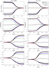Fig. A.1 Oscillation amplitudes of the spin Ω2 (top row), the lag angle δ2 (second row), the equatorial flattening ${\mathcal{E}}_2^{\rho }$ (third row), and polar flattening ${\mathcal{E}}_2^z$ (bottom row) of a Kepler-38-type planet around the pseudo-synchronous solution. The different colors indicate different methods of obtaining the amplitudes: numerical in black, analytical up to zeroth-order in green, up to third order in red, and our new simplified model in blue. The dashed black lines represent the numerical mean solution. The different columns represent different planetary eccentricities: e2 = 0.05 (left column) and e2 = 0.1 (right column).

And

$$\begin{array}{r}\hfill {\mathcal{E}}_{001}^z{}^c=\frac{3}{2}{ϵ}_2^{-\rho }\frac{{\gamma }_2^2}{{\gamma }_2^2+n_2^2};{\mathcal{E}}_{001}^z{}^s=\frac{3}{2}{ϵ}_2^{-\rho }\frac{n_2{\gamma }_2}{{\gamma }_2^2+n_2^2}\\ \hfill {\mathcal{E}}_{201}^z{}^c=\frac{45}{8}{ϵ}_2^{-\rho }\frac{{\gamma }_2^2}{{\gamma }_2^2+n_2^2};{\mathcal{E}}_{201}^z{}^s=\frac{45}{8}{ϵ}_2^{-\rho }\frac{n_2{\gamma }_2}{{\gamma }_2^2+n_2^2}\\ \hfill {\mathcal{E}}_{200}^z{}^c=\frac{15}{8}{ϵ}_2^{-\rho }\frac{{\gamma }_2^2{\mathcal{C}}_2+2(n_1-n_2){\gamma }_2{\mathcal{S}}_2}{{\gamma }_2^2+4{(n_1-n_2)}^2}\\ \hfill {\mathcal{E}}_{200}^z{}^s=\frac{15}{8}{ϵ}_2^{-\rho }\frac{2(n_1-n_2){\gamma }_2{\mathcal{C}}_2-{\gamma }_2^2{\mathcal{S}}_2}{{\gamma }_2^2+4{(n_1-n_2)}^2}\\ \hfill {\mathcal{E}}_{310}^z{}^c=\frac{225}{32}{ϵ}_2^{-\rho }\frac{{\gamma }_2^2{\mathcal{C}}_1-n_1{\gamma }_2{\mathcal{S}}_1}{{\gamma }_2^2+n_2^2}\\ \hfill {\mathcal{E}}_{310}^z{}^s=\frac{225}{32}{ϵ}_2^{-\rho }\frac{n_2{\gamma }_2{\mathcal{C}}_1+{\gamma }_2^2{\mathcal{S}}_1}{{\gamma }_2^2+n_2^2},\end{array}$$(A.7)

where

$$\begin{array}{ccc}{ϵ}_2^{-\rho }=\frac{15}{4}\frac{m_0+m_1}{m_2}\frac{{\mathcal{R}}_2^3}{a_2^3}& ;& {ϵ}_2^{-M}=\frac{5}{4}\frac{n_2^2+{\mathcal{R}}_2^3}{\mathcal{G}{m}_2}\simeq \frac{{ϸ}_2^{-\rho }}{3}\\ \kappa =3\frac{m_0+m_1}{m_0+m_1+m_2}{ϵ}_2^{-\rho }& & \\ {\mathcal{C}}_k=\cos k\Delta \varpi & ;& {\mathcal{S}}_k=\sin k\Delta \varpi .\end{array}$$(A.8)

In Figure A.1 we compare the oscillation amplitudes obtained with our simplified model (blue curves), with the numerical solutions (black curves) and also with the analytical solution presented in Zoppetti et al. (2021b) (red curves), considering different eccentricities for the CB planet in the different columns. We exclude the pure circular case (i.e., e₂ = 0) in this analysis since the presence of a secondary star prohibits this scenario from existing in reality. For completeness, we also include the amplitudes obtained with the 2BP simplification (green curves) in which the binary is considered as a unique body with mass equal to the sum of the masses of the stellar components, and the mean numerical solutions (dashed black curves).

From Figure A.1 we observe that our simplified analytical model not only represents very well our previous and more complex analytical model, but also is able to very accurately reproduce the oscillation amplitudes of all the parameters that characterize the rotational state. For this reason, in this work we employ the analytical approximation given in equation (A.1) with the coefficients given in the system (A.4)–(A.7) for characterizing the oscillation amplitudes of the CB planetary rotation in the pseudo-synchronous state.

References

All Tables

All Figures

	Fig. 1 Schematic of the 3BP from an inertial frame (O-frame) and from a m2 -relative frame.
In the text

	Fig. 2 Tidal evolution of the Jacobian semimajor axis (leftpanel), the eccentricity (center panel), and the difference of pericenters (right panel), for a pseudo-synchronous CB planet due to creep tides. Different relaxation factors γ2 are considered with different colors (see legend in center panel). The thick curves correspond to the low-pass filtered evolution.
In the text

Fig. 3 Secular orbital evolution of the semimajor axis (left panels) and eccentricity (right panels) of a pseudo-synchronous CB planet due to creep tides, as a function of its normalized relaxation factor. The solid curves are the results of a numerical averaging of the full evolution equations, while the dashed curves represent the results of our analytical secular model. Different α-values are used in the different rows and different planetary eccentricities are shown in the different colors. The region γ2/n2 > 1 approximately corresponds to the gaseous regime while the region γ2/n2 < 1 corresponds to the stiff regime.

In the text

	Fig. 4 Secular semimajor axis evolution of a pseudo-synchronous CB planet due to creep tides, as a function of its distance to the binary measured with α = a1/a2. In the different panels CB planets in different viscosity regimes are considered. The different types of curves and different colors are the same as those for Fig. 3.
In the text

Fig. A.1 Oscillation amplitudes of the spin Ω2 (top row), the lag angle δ2 (second row), the equatorial flattening ${\mathcal{E}}_2^{\rho }$ (third row), and polar flattening ${\mathcal{E}}_2^z$ (bottom row) of a Kepler-38-type planet around the pseudo-synchronous solution. The different colors indicate different methods of obtaining the amplitudes: numerical in black, analytical up to zeroth-order in green, up to third order in red, and our new simplified model in blue. The dashed black lines represent the numerical mean solution. The different columns represent different planetary eccentricities: e2 = 0.05 (left column) and e2 = 0.1 (right column).

In the text

References

- Benítez-Llambay, P., Masset, F., & Beaugé, C. 2011, A&A, 528, A2 [NASA ADS] [CrossRef] [EDP Sciences] [Google Scholar]
- Beutler, G. 2005, Methods of Celestial Mechanics (Berlin: Springer), I, 99 [NASA ADS] [Google Scholar]
- Correia, A. C. M., Boué, G., Laskar, J., et al. 2014, A&A, 571, A50 [NASA ADS] [CrossRef] [EDP Sciences] [Google Scholar]
- Correia, A. C. M., Boué, G., & Laskar, J. 2016, Celest. Mech. Dyn. Astron., 126, 189 [NASA ADS] [CrossRef] [Google Scholar]
- Doyle, L. R., Carter, J. A., Fabrycky, D. C., et al. 2011, Science, 333, 1602 [NASA ADS] [CrossRef] [Google Scholar]
- Efroimsky, M. 2012, ApJ, 746, 150 [Google Scholar]
- Efroimsky, M. 2015, AJ, 150, 98 [NASA ADS] [CrossRef] [Google Scholar]
- Ferraz-Mello, S. 2013, Celest. Mech. Dyn. Astron., 116, 109 [Google Scholar]
- Ferraz-Mello, S. 2015a, Celest. Mech. Dyna. Astron., 122, 359 [NASA ADS] [CrossRef] [Google Scholar]
- Ferraz-Mello, S. 2015b, A&A, 579, A97 [NASA ADS] [CrossRef] [EDP Sciences] [Google Scholar]
- Ferraz-Mello, S., Rodríguez, A., & Hussmann, H. 2008, Celest. Mech. Dyn. Astron., 101, 171 [Google Scholar]
- Folonier, H. A., Ferraz-Mello, S., & Andrade-Ines, E. 2018, Celest. Mech. Dyn. Astron., 130, 78 [Google Scholar]
- Holman, M. J., & Wiegert, P. A. 1999, AJ, 117, 621 [Google Scholar]
- Hut, P. 1981, A&A, 99, 126 [NASA ADS] [Google Scholar]
- Kostov, V. B., McCullough, P. R., Carter, J. A., et al. 2014, ApJ, 784, 14 [NASA ADS] [CrossRef] [Google Scholar]
- Kostov, V. B., Orosz, J. A., Welsh, W. F., et al. 2016, ApJ, 827, 86 [NASA ADS] [CrossRef] [Google Scholar]
- Kostov, V. B., Orosz, J. A., Feinstein, A. D., et al. 2020, AJ, 159, 253 [Google Scholar]
- Lainey, V., Arlot, J.-E., Karatekin, Ö., et al. 2009, Nature, 459, 957 [NASA ADS] [CrossRef] [Google Scholar]
- MacDonald, G. J. F. 1964, Rev. Geophys. Space Phys., 2, 467 [Google Scholar]
- Michtchenko, T. A., & Malhotra, R. 2004, Icarus, 168, 237 [Google Scholar]
- Mignard, F. 1979, Moon Planets, 20, 301 [Google Scholar]
- Mills, S. M., & Mazeh, T. 2017, ApJ, 839, L8 [Google Scholar]
- Moriwaki, K., & Nakagawa, Y. 2004, ApJ, 609, 1065 [NASA ADS] [CrossRef] [Google Scholar]
- Orosz, J. A., Welsh, W. F., Carter, J. A., et al. 2012a, ApJ, 758, 87 [Google Scholar]
- Orosz, J. A., Welsh, W. F., Carter, J. A., et al. 2012b, Science, 337, 1511 [Google Scholar]
- Orosz, J. A., Welsh, W. F., Haghighipour, N., et al. 2019, AJ, 157, 174 [NASA ADS] [CrossRef] [Google Scholar]
- Paardekooper, S.-J., Leinhardt, Z. M., Thébault, P., et al. 2012, ApJ, 754, L16 [NASA ADS] [CrossRef] [Google Scholar]
- Renaud, J. P., & Henning, W. G. 2018, ApJ, 857, 98 [Google Scholar]
- Schwamb, M. E., Orosz, J. A., Carter, J. A., et al. 2013, ApJ, 768, 127 [Google Scholar]
- Socia, Q. J., Welsh, W. F., Orosz, J. A., et al. 2020, AJ, 159, 94 [Google Scholar]
- Welsh, W. F., Orosz, J. A., Carter, J. A., et al. 2012, Nature, 481, 475 [Google Scholar]
- Welsh, W. F., Orosz, J. A., Short, D. R., et al. 2015, ApJ, 809, 26 [Google Scholar]
- Zombeck, M. 2007, Handbook of Space Astronomy and Astrophysics, 3rd edn. (Cambridge: Cambridge University Press) [Google Scholar]
- Zoppetti, F. A., Beaugé, C., & Leiva, A. M. 2018, MNRAS, 477, 5301 [Google Scholar]
- Zoppetti, F. A., Beaugé, C., Leiva, A. M., et al. 2019a, A&A, 627, A109 [NASA ADS] [CrossRef] [EDP Sciences] [Google Scholar]
- Zoppetti, F. A., Beaugé, C., & Leiva, A. M. 2019b, J. Phys. Conf. Ser., 1365, 012029 [Google Scholar]
- Zoppetti, F. A., Leiva, A. M., & Beaugé, C. 2020, A&A, 634, A12 [EDP Sciences] [Google Scholar]
- Zoppetti, F. A., Folonier, H., Leiva, A. M., et al. 2021a, A&A, 651, A49 [NASA ADS] [CrossRef] [EDP Sciences] [Google Scholar]
- Zoppetti, F. A., Folonier, H., Leiva, A. M. et al. 2021b, Proc. Int. Astron. Union 15, 252 [Google Scholar]
All Tables
Initial conditions of our reference numerical simulation, representing a Kepler-38-type system.
Physical and orbital parameters of confirmed circumbinary systems, and tidal parameters estimated with our model.