© The Authors 2023

1 Introduction

In general, Earth-mass planets are believed to be composed of a large rocky mantle covered by a thin atmospheric layer (e.g., Komacek & Abbot 2019; Wordsworth & Kreidberg 2022), as for the Earth, Venus, and Mars in the Solar System. The molecules that make up the atmospheres can absorb part of the radiation they receive from the host star, giving rise to local temperature gradients, which in turn create pressure variations. As a result, large-scale periodic mass redistribution inside the atmosphere occurs, while it attempts to return to an equilibrium state, known as thermal atmospheric tides.

Observations on Earth and Mars show that the pressure variations can be essentially decomposed in a diurnal and a semidiurnal tidal wave (e.g., Withers et al. 2011; Auclair-Desrotour et al. 2017). These oscillations are one of the most regular meteorological phenomena on Earth, and they are easily detectable by any station around the world (e.g., Chapman & Lindzen 1970). The thermal inertia of the atmosphere introduces a delay between the stellar heating and the thermal response, which creates an asymmetry in the mass redistribution with respect to the substellar point. As a consequence, the gravitational pull of the star exerts a torque on the atmosphere. The diurnal wave has no net torque, but the semidiurnal wave gives rise to angular momentum exchanges within the atmosphere (e.g., Correia & Laskar 2003a).

Thermal atmospheric tides garnered special interest with the discovery of the retrograde rotation of Venus (e.g., Carpenter 1964). Because the atmosphere and the mantle are usually well coupled by friction at the surface, the variations in the angular momentum of the atmosphere are then transferred to the mantle of the planet, modifying its spin. To explain the peculiar rotation of Venus, Gold & Soter (1969) thus proposed that it can be the result of a balance between bodily tides (i.e., gravitational tides raised in the mantle), which drive the planet toward synchronous rotation, and thermal tides, which drive it away. This effect is negligible on Earth, because it is too distant from the Sun; however, for Earth-like planets in the habitable zone of K-dwarf stars, thermal tides can lead to asynchronous equilibria similar to that of Venus (Leconte et al. 2015).

Formation studies predict that Earth-mass planets are common around main sequence dwarf stars (e.g., Schlecker et al. 2021). Indeed, there is already a large population of detected low-mass exoplanets, and their number is likely to grow rapidly (e.g., Winn 2018). These planets are found in a wide range of orbital configurations, from very eccentric to compact multibody resonant orbits (e.g., Borucki et al. 2013). We thus need a correct modeling of their spins and orbital dynamics. The estimates for the tidal evolution of a planet are based on a general formulation of the tidal potential (e.g., Kaula 1964). The classical expansion of this potential in elliptical elements depends on the chosen frame and introduces multiple index summations, which can lead to confusion and errors in the equations of motion. Moreover, mistakes such as neglecting energy or momentum conservation considerations are more easily done (Boué & Efroimsky 2019). For bodily tides, it has been shown that the equations of motion are more easily expressed in terms of angular momentum vectors (e.g., Correia & Valente 2022). Therefore, in this paper, we aim to also use these vectors to study the dynamics of a planet undergoing thermal tides. This formalism is independent of the reference frame and allows us to simply add the contributions of multiple bodies in the system.

In Sect. 2, we obtain the tidal potential of a planet whose atmosphere is excited through thermal forcing. In Sect. 3, we derive the equations of motion to study the spin and orbital evolution of a planet-star system under the action of thermal tides. In Sect. 4, we average the equations of motion over the mean anomaly and the argument of the pericenter, which provide simpler expressions that are easy to implement and suitable for long-term evolution studies. In Sects. 5 and 6, we provide the equations of motion in the simplified cases of small eccentricity, and planar motion, respectively. Finally, the last section is devoted to the conclusions.

2 Thermal atmospheric tides

We consider a planet with total mass m, which is composed of a perfectly spherical mantle with radius R, and a thin atmosphere with mass ℳ. We assume that the mantle is completely rigid, while the atmosphere can be deformed owing to the thermal forcing from the radiation of a nearby star.

2.1 Atmospheric tidal potential

The gravitational potential in a generic point of the space, r, at a given time, t, generated by all the particles that compose the atmosphere is given by (e.g., Goldstein 1950) $$V\left(r,t\right)=-𝒢{\displaystyle {\int }_{ℳ}\frac{dℳ}{\left|r-r\prime \right|},}$$(1)

where r′ is the position of an atmosphere mass element dℳ. For a frame centered in the planet, we can expand Eq. (1) in Legendre polynomials, P_ℓ(x), as $$V\left(r,t\right)={\displaystyle \sum _{\ell =0}^{\infty }{V}_{\ell }\left(r,t\right)},$$(2)

with $$V_{\ell }\left(r,t\right)=-\frac{𝒢}{r}{\displaystyle {\int }_{ℳ}{\left(\frac{r\prime }{r}\right)}^{\ell }{P}_{\ell }\left(\widehat{r}\cdot \widehat{r}\prime \right)\text{\hspace{0.17em}d}ℳ},$$(3)

where $\widehat{r}=r/r$ is the unit vector and r = ∥r∥ is the norm, and we assume r > r′. For ℓ = 0 and ℓ = 1, we have $P_0\left(\widehat{r}\cdot \widehat{r}\prime \right)=1$ and $P_1\left(\widehat{r}\cdot \widehat{r}\prime \right)=\widehat{r}\cdot \widehat{r}\prime$, respectively, and thus we can rewrite $$V_0\left(r,t\right)=-\frac{𝒢ℳ}{r}$$(4)

and $$V_1\left(r,t\right)=-\frac{𝒢ℳ}{r^2}\widehat{r}\cdot r_{\text{cm}},$$(5)

where $$r_{\text{cm}}=\frac{1}{ℳ}{\displaystyle {\int }_{ℳ}r\prime }\text{\hspace{0.17em}d}ℳ,$$(6)

is the center of mass of the atmosphere. Furthermore, V₀ is the potential of a spherical symmetric atmosphere, which can be absorbed in the total potential of a point-mass planet. For simplicity, we can set r_cm = 0, and thus V₁ = 0. The resulting potential of a perturbed atmosphere, also known as tidal potential, is then given by the differential potential $$\text{Δ}V\left(r,t\right)=V\left(r,t\right)-V_0\left(r,t\right)-V_1\left(r,t\right)={\displaystyle \sum _{\ell =2}^{\infty }{V}_{\ell }}\left(r,t\right).$$(7)

Moreover, if we assume r ≫ r′, we can keep only the term in ℓ = 2 (quadrupolar approximation), and finally get $$\text{Δ}V\left(r,t\right)\approx V_2\left(r,t\right)=-\frac{𝒢}{r^3}{\displaystyle {\int }_{ℳ}r\prime P_2\left(\widehat{r}\cdot \widehat{r}\prime \right)\text{\hspace{0.17em}d}ℳ}.$$(8)

2.2 Deformation of the atmosphere

For a frame attached to the planet, we can express r = (r, θ, φ) and r′ = (r′, θ′, φ′) in spherical coordinates. Then $$\text{d}ℳ\text{\hspace{0.17em}=\hspace{0.17em}}{\rho }_a\left(r\prime ,t\right)r{\prime }^2\text{d}t\prime \text{\hspace{0.17em}dΩ}\prime ,$$(9)

where ρ_a(r′, t) is the local density of the atmosphere, and $$\text{dΩ}\prime =\text{sin\hspace{0.17em}}\theta \prime \text{d}\theta \prime \text{\hspace{0.17em}d}\varphi \prime$$(10)

is the differential solid angle. Assuming a constant radius for the planet, R, we have $$\text{Δ}V\left(r,t\right)=-\frac{𝒢}{r^3}{\displaystyle \underset{r\prime =R}{\overset{+\infty }{\int }}{\displaystyle \underset{\varphi \prime =0}{\overset{2\pi }{\int }}{\displaystyle \underset{\theta \prime =0}{\overset{\pi }{\int }}{\rho }_a\left(r\prime ,t\right)r{\prime }^4{P}_2\left(\widehat{r}\cdot \widehat{r}\prime \right)\text{\hspace{0.17em}d}r\prime }\text{\hspace{0.17em}dΩ}\prime },}$$(11)

with $$\widehat{r}\cdot \widehat{r}\prime =\text{cos\hspace{0.17em}}\theta \text{\hspace{0.17em}cos\hspace{0.17em}}\theta \prime +\text{sin\hspace{0.17em}}\theta \text{\hspace{0.17em}sin\hspace{0.17em}}\theta \prime \text{\hspace{0.17em}cos}\left(\varphi -\varphi \prime \right).$$(12)

For terrestrial planets, the height of the atmosphere, H, is usually negligible compared to the radius of the planet¹, that is $$\begin{array}{ccc}R\le r\prime \le R+H,& \text{and}& \frac{H}{R}\ll 1\end{array}.$$(13)

Thus, we can take a thin layer approximation and get $$\text{Δ}V\left(r,t\right)=-𝒢R{\left(\frac{R}{r}\right)}^3{\displaystyle \underset{r\prime =R}{\overset{R+H}{\int }}{\displaystyle \underset{\varphi \prime =0}{\overset{2\pi }{\int }}{\displaystyle \underset{\theta \prime =0}{\overset{\pi }{\int }}{\rho }_a\left(r\prime ,t\right)P_2\left(\widehat{r}\cdot \widehat{r}\prime \right)\text{\hspace{0.17em}d}r\prime \text{\hspace{0.17em}dΩ}\prime }.}}$$(14)

We further assume that the self-gravity fluctuations in the atmosphere can also be neglected (e.g., Cowling 1941). Then, we use the hydrostatic equilibrium equation, $$\text{d}p=-{\rho }_a\left(r\prime ,t\right)g\left(r\prime \right)\text{d}r\prime ,$$(15)

where p(r′, t) is the local pressure and g(r′) is the local gravity, to eliminate the integral in height $$\text{Δ}V\left(r,t\right)=-\frac{𝒢R}{g}{\left(\frac{R}{r}\right)}^3{\displaystyle \underset{\varphi \prime =0}{\overset{2\pi }{\int }}{\displaystyle \underset{\theta \prime =0}{\overset{\pi }{\int }}{p}_s\left(\theta \prime ,\varphi \prime ,t\right)P_2\left(\widehat{r}\cdot \widehat{r}\prime \right)\text{\hspace{0.17em}\hspace{0.17em}dΩ}\prime ,}}$$(16)

and where p_s(θ′, φ′, t) = p(R, θ′, φ′, t) is the surface pressure. We also assume that p(R + H, θ′, φ′, t) = 0, and that g(r′) = g(R) = g is constant. In a very general formulation, the surface pressure depends on the amount of energy per unit area received from the star, that is, the insolation W(θ′, φ′, t), $$p_s\left(\theta \prime ,\varphi \prime ,t\right)=F\left[W\left(\theta \prime ,\varphi \prime ,t\right)\right],$$(17)

with F being an operator that depends on the composition and the physical properties of the atmosphere. The insolation W can be seen as a forcing function. For a measurement at the top of the atmosphere, the insolation is given by (e.g., Ward 1974) $$W\left(\theta \prime ,\varphi \prime ,t\right)={\mathcal{𝒮}}_{\star }{\left(\frac{a}{r_{\star }}\right)}^2\{\begin{array}{cc}\widehat{r}\prime \cdot {\widehat{r}}_{\star }& \widehat{r}\prime \cdot {\widehat{r}}_{\star }>0\\ 0,& \widehat{r}\prime \cdot {\widehat{r}}_{\star }\le 0\end{array},$$(18)

where S_* = L_*+(4πa²) is the “solar” constant, L_* is the luminosity of the star, r_* is the position of the star with respect to the center of mass of the planet (which is a function of the time), a is the semimajor axis of the star-planet orbit, and $$\widehat{r}\prime \cdot {\widehat{r}}_{\star }=\text{cos\hspace{0.17em}}\theta \prime \text{\hspace{0.17em}cos\hspace{0.17em}}{\theta }_{\star }+\text{sin\hspace{0.17em}}\theta \prime \text{\hspace{0.17em}sin\hspace{0.17em}}{\theta }_{\star }\text{\hspace{0.17em}cos}\left(\varphi \prime -{\varphi }_{\star }\right).$$(19)

We can expand expression (18) in Legendre polynomials, as $$W\left(\theta \prime ,\varphi \prime ,t\right)={\displaystyle \sum _{n=0}^{\infty }{W}_n{\text{Θ}}_n\left(r\prime ,t\right),}$$(20)

with $${\text{Θ}}_n\left(r,t\right)={\left(\frac{a}{r_{\star }}\right)}^2{P}_n\left(\widehat{r}\cdot {\widehat{r}}_{\star }\right),$$(21)

and $$W_n={𝒮}_{\star }\frac{2n+1}{2}{\displaystyle {\int }_0^{1}x{P}_n\left(x\right)\text{\hspace{0.17em}d}x.}$$(22)

The insolation variations can also be expressed in the frequency domain by performing a Fourier transform $$W\left(\theta \prime ,\varphi \prime ,t\right)={\displaystyle \sum _{n=0}^{\infty }{\displaystyle \int W_n{\widehat{\text{Θ}}}_n\left(r\prime ,\sigma \right){\text{e}}^{\text{i}\sigma \text{t}}}}\text{\hspace{0.17em}d}\sigma ,$$(23)

with $${\widehat{\text{Θ}}}_n\left(r,\sigma \right)={\displaystyle \int {\text{Θ}}_n}\left(r,t\right){\text{e}}^{-\text{i}\sigma \text{t}}\text{\hspace{0.17em}d}t.$$(24)

Since the Legendre polynomials form an orthogonal basis, any other quantity with the same symmetry as the insolation, such as the surface pressure variations (Eq. (17)), can also be expanded in a similar way. Therefore, we write $$p_s\left(\theta \prime ,\varphi \prime ,t\right)={\displaystyle \sum _{n=0}^{\infty }{{\displaystyle \int {\widehat{p}}_n\left(\sigma \right)\widehat{\text{Θ}}}}_n\left(r\prime ,\sigma \right){\text{e}}^{i\sigma t}\text{\hspace{0.17em}d}\sigma },$$(25)

where ${\widehat{p}}_n$ are the coefficients of order n of the decomposition of the surface pressure in Legendre polynomials. They can also be expressed in terms of spherical harmonics $Y_{\ell }^m$ and their complex conjugate ${\overline{Y}}_{\ell }^m$ (e.g., Abramowitz & Stegun 1972) $$P_{\ell }\left(\widehat{r}\cdot \widehat{r}\prime \right)=\frac{4\pi }{2\ell +1}{\displaystyle \sum _{M=-\ell }^{\ell }{Y}_{\ell }^m\left(\theta ,\varphi \right){\overline{Y}}_{\ell }^m\left(\theta \prime ,\varphi \prime \right)}.$$(26)

Then, by replacing (25) and (26) in expression (16) we get $$\begin{array}{l}\text{Δ}V\left(r,t\right)=-\frac{𝒢R}{g}{\left(\frac{R}{r}\right)}^3\frac{4\pi }{5}{\displaystyle \sum _{m=-2}^2{Y}_2^m\left(\theta ,\varphi \right){\displaystyle \sum _{n=0}^{\infty }{\displaystyle \int {\widehat{p}}_n\left(\sigma \right)}}}\hfill \\ \times {\displaystyle \underset{\varphi \prime =0}{\overset{2\pi }{\int }}{\displaystyle \underset{\theta \prime =0}{\overset{\pi }{\int }}{\widehat{\text{Θ}}}_n\left(r\prime ,\sigma \right){\overline{Y}}_2^m}\left(\theta \prime ,\varphi \prime \right)\text{\hspace{0.17em}dΩ}\prime {\text{e}}^{\text{iσ}t}}\text{\hspace{0.17em}d}\sigma \text{,}\hfill \end{array}$$(27)

and, using the orthogonality formula $${\displaystyle \underset{\varphi \prime =0}{\overset{2\pi }{\int }}{\displaystyle \underset{\theta \prime =0}{\overset{\pi }{\int }}{P}_n\left(\widehat{r}\prime \cdot {\widehat{r}}_{\star }\right){\overline{Y}}_2^m\left(\theta \prime ,\varphi \prime \right)\text{\hspace{0.17em}dΩ}\prime }=\frac{4\pi }{5}{\overline{Y}}_2^m\left({\theta }_{\star },{\varphi }_{\star }\right){\delta }_{n,2}},$$(28)

where δ_n,2 is the Kronecker delta, we finally get $$\text{Δ}V\left(r,t\right)=-\frac{𝒢R}{g}{\left(\frac{R}{r}\right)}^3\frac{4\pi }{5}{\displaystyle \int {\widehat{p}}_2\left(\sigma \right){\widehat{\text{Θ}}}_2\left(r,\sigma \right){\text{e}}^{\text{i}\sigma t}}\text{\hspace{0.17em}d}\sigma .$$(29)

The mass distribution inside the planet is usually better characterized by its inertia tensor. Then, we can rearrange Eq. (29) as $$\text{Δ}V\left(r_B,t\right)=\frac{3G}{2r^3}{\widehat{r}}_B\cdot {ℐ}_B\left(t\right)\cdot {\widehat{r}}_B,$$(30)

with $${ℐ}_B\left(t\right)={\displaystyle \int {\widehat{p}}_2\left(\sigma \right){\widehat{\text{Λ}}}_B}\left(\sigma \right){\text{e}}^{\text{i}\sigma t}\text{\hspace{0.17em}d}\sigma ,$$(31) $${\widehat{\text{Λ}}}_B\left(\sigma \right)={\displaystyle \int {\text{Λ}}_B\left(t\right){\text{e}}^{-i\sigma t}\text{\hspace{0.17em}d}t,}$$(32)

and $${\text{Λ}}_B\left(t\right)=\frac{4\pi R^4}{5g}{\left(\frac{a}{r_{\star }}\right)}^2\left({\widehat{r}}_{\star }{}_B{\widehat{r}}_{\star B}^T-\frac{1}{3}\text{𝕀}\right),$$(33)

where ^T denotes the transpose, 𝕀 is the identity matrix, ℐ(t) is the atmosphere inertia tensor that accounts for the departure of the mass distribution from a sphere (Eq. (56)), while Λ(t) is a forcing tensor that depends on time through r_*. The subscript _B is there to remind us that Eqs. (30)–(33) were obtained in the body frame, that is, in a frame attached to the planet.

2.3 Deformation in an arbitrary frame

It is also possible to compute the deformation of the atmosphere in an arbitrary frame, I(t). Following Correia & Valente (2022), we let 𝒮 be the rotation matrix that allows us to convert any vector r_B in a frame attached to the planet into another frame r, such that r = 𝒮 r_B, and $$ℐ\left(t\right)=𝒮\left(t\right){ℐ}_B\left(t\right)𝒮{\left(t\right)}^T.$$(34)

Then, the atmospheric tidal potential (Eq. (30)) becomes $$\text{Δ}V\left(r,t\right)=\frac{3𝒢}{2r^3}\widehat{r}\cdot ℐ\left(t\right)\cdot \widehat{r}.$$(35)

Similarly, we can also compute the forcing tensor (Eq. (33)) in the new frame as $$\text{Λ}\left(t\right)=𝒮\left(t\right){\text{Λ}}_B\left(t\right)𝒮{\left(t\right)}^T=-\frac{4\pi R^4}{5g}{\left(\frac{a}{r_{\star }}\right)}^2\left({\widehat{r}}_{\star }{\widehat{r}}_{\star }^T-\frac{1}{3}\text{𝕀}\right).$$(36)

We note that the expression of I_B(t) (Eq. (31)) also corresponds to the convolution product between ${\tilde{p}}_2\left(t\right)$ and Λ_B(t), $${ℐ}_B\left(t\right)=\left[{\tilde{p}}_2*{\text{Λ}}_B\right]\left(t\right)={\displaystyle \int {\tilde{p}}_2\left(t-t\prime \right){\text{Λ}}_B\left(t\prime \right)\text{\hspace{0.17em}d}t\prime },$$(37)

where $${\tilde{p}}_2\left(t\right)={\displaystyle \int {\widehat{p}}_2\left(\sigma \right){\text{e}}^{\text{i}\sigma \text{t}}\text{\hspace{0.17em}d}\sigma }.$$(38)

Then, in the frequency domain we have $$\begin{array}{l}\widehat{ℐ}\left(\sigma \right)={\displaystyle \int ℐ\left(t\right){\text{e}}^{-\text{i}\sigma t}\text{\hspace{0.17em}d}t={\displaystyle \int 𝒮\left(t\right){ℐ}_B\left(t\right)𝒮{\left(t\right)}^T{\text{e}}^{-\text{i}\sigma t}\text{\hspace{0.17em}d}t}}\hfill \\ ={\displaystyle \int {\displaystyle \int {\tilde{p}}_2\left(t-t\prime \right)𝒮\left(t\right){\text{Λ}}_B\left(t\prime \right)𝒮{\left(t\right)}^T{\text{e}}^{-\text{i}\sigma t}\text{\hspace{0.17em}d}t\prime \text{d}t}}\hfill \\ ={\displaystyle \int {\displaystyle \int {\tilde{p}}_2\left(\tau \right)𝒮\left(t\prime +\tau \right){\text{Λ}}_B\left(t\prime \right)𝒮{\left(t\prime +\tau \right)}^T{\text{e}}^{-\text{i}\sigma \left(t\prime +\tau \right)}\text{\hspace{0.17em}d}t\prime \text{d}\tau }.}\hfill \end{array}$$(39)

Since 𝒮(t) is a rotation matrix, we note that 𝒮(t′ + τ) = 𝒮(τ)𝒮(t′), and thus $$\begin{array}{l}\widehat{ℐ}\left(\sigma \right)={\displaystyle \int {\displaystyle \int {\tilde{p}}_2\left(\tau \right)𝒮\left(\tau \right)\text{\hspace{0.17em}Λ}\left(t\prime \right)𝒮{\left(\tau \right)}^T{\text{e}}^{-\text{i}\sigma \left(t\prime +\tau \right)}\text{\hspace{0.17em}d}t\prime \text{\hspace{0.17em}d}\tau }}\hfill \\ ={\displaystyle \int {\tilde{p}}_2\left(\tau \right)𝒮\left(\tau \right)\widehat{\text{Λ}}\left(\sigma \right)𝒮{\left(\tau \right)}^T{\text{e}}^{-\text{i}\sigma \tau }\text{\hspace{0.17em}d}\tau },\hfill \end{array}$$(40)

with $$\widehat{\text{Λ}}\left(\sigma \right)={\displaystyle \int \text{Λ}\left(t\right)}{\text{e}}^{-\text{i}\sigma t}\text{d}t.$$(41)

At this stage, we need to adopt a specific frame to proceed, in order to express 𝒮(τ). We adopt here a Cartesian reference frame (p, q, s), such that s is the spin axis, $$p=\frac{k\times s}{\sin \epsilon },q=\frac{k-\cos \epsilon s}{\sin \epsilon },\cos \epsilon =k\cdot s,$$(42)

where k is a unit vector that is normal to the orbital plane of the star, p is aligned with the line of nodes between the equator of the planet and the orbital plane, and ε is the angle between these two planes, also known as the obliquity (Fig. 1). This particular frame is very useful to obtain the secular equations of motion (Sect. 4.2), as it allows us to decouple the rotational perturbations from the orbital ones (Correia 2006). For a planet rotating about the s axis with angular velocity ω, we thus have $$𝒮\left(\tau \right)=\left[\begin{array}{ccc}\cos \omega \tau & -\sin \omega \tau & 0\\ \sin \omega \tau & \cos \omega \tau & 0\\ 0& 0& 1\end{array}\right].$$(43)

The result for the product $𝒮\left(\tau \right)\widehat{\text{Λ}}\left(\sigma \right)𝒮{\left(\tau \right)}^T$ is given in Table 1. For instance, for the ${\widehat{I}}_{23}\left(\sigma \right)$ coefficient of the inertia tensor $\widehat{ℐ}\left(\sigma \right)$ (Eq. (57)), we then finally have $$\begin{array}{l}{\widehat{I}}_{23}\left(\sigma \right)={\displaystyle \int {\tilde{p}}_2\left(\tau \right)}\left[{\widehat{\text{Λ}}}_{13}\left(\sigma \right)\sin \omega \tau +{\widehat{\text{Λ}}}_{23}\left(\sigma \right)\cos \omega \tau \right]{\text{e}}^{-\text{i}\sigma \tau }\text{d}\tau \hfill \\ ={\widehat{\text{Λ}}}_{13}\left(\sigma \right){\displaystyle \int {\tilde{p}}_2\left(\tau \right)}\sin \omega \tau {\text{e}}^{-\text{i}\sigma \tau }\text{d}\tau \hfill \\ +{\widehat{\text{Λ}}}_{23}\left(\sigma \right){\displaystyle \int {\tilde{p}}_2}\left(\tau \right)\cos \omega \tau {\text{e}}^{-\text{i}\sigma \tau }\text{d}\tau \hfill \\ =\frac{1}{2}{\widehat{p}}_2\left(\sigma -\omega \right)\left[{\widehat{\text{Λ}}}_{23}\left(\sigma \right)-{\text{i}\widehat{\text{Λ}}}_{13}\left(\sigma \right)\right]\hfill \\ +\frac{1}{2}{\widehat{p}}_2\left(\sigma +\omega \right)\left[{\widehat{\text{Λ}}}_{23}\left(\sigma \right)+{\text{i}\widehat{\text{Λ}}}_{13}\left(\sigma \right)\right].\hfill \end{array}$$(44)

Similarly, for the remaining coefficients of $\widehat{ℐ}\left(\sigma \right)$, we obtain $$\begin{array}{l}{\widehat{I}}_{13}\left(\sigma \right)=\frac{1}{2}{\widehat{p}}_2\left(\sigma -\omega \right)\left[{\widehat{\text{Λ}}}_{13}\left(\sigma \right)+\text{i\hspace{0.17em}}{\widehat{\text{Λ}}}_{23}\left(\sigma \right)\right]\hfill \\ +\frac{1}{2}{\widehat{p}}_2\left(\sigma +\omega \right)\left[{\widehat{\text{Λ}}}_{13}\left(\sigma \right)-{\text{i}\widehat{\text{Λ}}}_{23}\left(\sigma \right)\right],\hfill \end{array}$$(45) $$\begin{array}{l}{\widehat{I}}_{12}\left(\sigma \right)=\frac{1}{2}{\widehat{p}}_2\left(\sigma -2\omega \right)\left[{\widehat{\text{Λ}}}_{12}\left(\sigma \right)+\text{iΔ\hspace{0.17em}}\widehat{\text{Λ}}\left(\sigma \right)\right]\hfill \\ +\frac{1}{2}{\widehat{p}}_2\left(\sigma +2\omega \right)\left[{\widehat{\text{Λ}}}_{12}\left(\sigma \right)-\text{iΔ}\widehat{\text{Λ}}\left(\sigma \right)\right],\hfill \end{array}$$(46) $${\widehat{I}}_{33}\left(\sigma \right)={\widehat{p}}_2\left(\sigma \right){\widehat{\text{Λ}}}_{33}\left(\sigma \right),$$(47) $${\widehat{I}}_{22}\left(\sigma \right)=\text{Δ}\widehat{I}\left(\sigma \right)-\frac{1}{2}{\widehat{I}}_{33}\left(\sigma \right),$$(48) $${\widehat{I}}_{11}\left(\sigma \right)=-\text{Δ}\widehat{I}\left(\sigma \right)-\frac{1}{2}{\widehat{I}}_{33}\left(\sigma \right)$$(49)

with $$\begin{array}{l}\text{Δ}\widehat{I}\left(\sigma \right)=\frac{1}{2}{\widehat{p}}_2\left(\sigma -2\omega \right)\left[\text{Δ}\widehat{\text{Λ}}\left(\sigma \right)-{\text{i}\widehat{\text{Λ}}}_{12}\left(\sigma \right)\right]\hfill \\ +\frac{1}{2}{\widehat{p}}_2\left(\sigma +2\omega \right)\left[\text{Δ}\widehat{\text{Λ}}\left(\sigma \right)+{\text{i}\widehat{\text{Λ}}}_{12}\left(\sigma \right)\right],\hfill \end{array}$$(50)

and $$\text{Δ}\widehat{\text{Λ}}\left(\sigma \right)=\frac{1}{2}\left[{\widehat{\text{Λ}}}_{22}\left(\sigma \right)-{\widehat{\text{Λ}}}_{11}\left(\sigma \right)\right].$$(51)

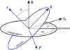Fig. 1 Reference frame (p, q, s) and angles. We note that k is a unit vector that is normal to the orbital plane, s is a unit vector that is normal to the equatorial plane of the planet, and p is a unit vector along the line of nodes of the two planes. The obliquity ε is the angle between the two planes, ϖ is the argument of the pericenter, and υ is the true anomaly.

2.4 Surface pressure variations

The deformation of the atmosphere is given by the inertia tensor, $\widehat{ℐ}\left(\sigma \right)$, which is obtained from the second harmonic of the surface pressure, ${\widehat{p}}_2\left(\sigma \right)$, combined with the forcing tensor, $\widehat{\text{Λ}}\left(\sigma \right)$ (Eq. (40)). While the forcing tensor is well determined, as it only depends on the position of the star (Eq. (36)), the surface pressure is subject to many uncertainties, as it depends on the composition and the physical properties of the atmosphere.

In order to compute ${\widehat{p}}_2\left(\sigma \right)$, we need to adopt some dynamical model for the atmosphere. The study of thermal tides has been initiated by the pioneer work of Siebert (1961) and Chapman & Lindzen (1970). They assumed that the atmosphere of the planet corresponds to an ideal gas obeying the perfect gas law, together with the conservation of mass and the Navier-Stokes equation. These equations were then linearized around the equilibrium state. Chapman & Lindzen (1970) studied the case of a fast rotating planet, such as the Earth, but for long-term evolution studies, the planet may encounter slow rotation regimes near synchronization, such as Venus (e.g., Correia & Laskar 2001, 2003b). In the later case, it is important to take into account the effect of radiative losses (Auclair-Desrotour et al. 2017). Assuming a slowly rotating convective atmosphere, the hydrodynamic equations can be simplified drastically, since the Coriolis acceleration can be neglected. The thin atmospheric layer close to the surface has a strongly negative temperature gradient (Seiff et al. 1980), which subjects this layer to convective instability (Baker et al. 2000). As a result, gravity waves cannot propagate in the unstable region above the surface and we can set the Brunt-Väisälä frequency to approximately zero, which corresponds to the adiabatic temperature gradient. Following Dobrovolskis & Ingersoll (1980), thermal tides are thus solely considered to be generated by the average heat at the ground, ${\widehat{J}}_0$, which finally gives the following for the second harmonic of the surface pressure variations (Auclair-Desrotour et al. 2017, Eq. (166)): $${\widehat{p}}_2\left(\sigma \right)=-\frac{\kappa {\rho }_0{\widehat{J}}_0}{{\sigma }_0+\text{i}\sigma },$$(52)

with κ = 1 − γ⁻¹, where γ is the adiabatic exponent, ρ₀ = ρ_a(0) is the mean surface density of the atmosphere, and σ₀ is the radiative frequency of the atmosphere, which depends on its thermal capacity. This theoretical estimation agrees incredibly well with empirical estimations derived from generic global climate circulation models (Leconte et al. 2015, Fig. 1). Interestingly, it is also similar to the Love number of a Maxwell tidal model (e.g., Correia et al. 2014; Auclair-Desrotour et al. 2019). The minus sign in the expression of ${\widehat{p}}_2\left(\sigma \right)$ causes the pressure variations to lead the star, a phenomenon well documented for the Earth (e.g., Chapman & Lindzen 1970).

The ${\widehat{p}}_2\left(\sigma \right)$ is a complex number, whose modulus gives the amplitude of the pressure variations and the argument gives the phase lag between the substellar point and the maximal deformation of the atmosphere. It can be decomposed in its real and imaginary parts as $${\widehat{p}}_2\left(\sigma \right)=a\left(\sigma \right)-\text{i}b\left(\sigma \right),$$(53)

which is very useful when we write the secular equations of motion (see Sect. 4.2), because the imaginary part characterizes the atmosphere′s viscous response. We thus have $$a\left(\sigma \right)=-\frac{\kappa {\rho }_0{\widehat{J}}_0{\sigma }_0}{{\sigma }_0{}^2+{\sigma }^2},\text{\hspace{0.17em}\hspace{0.17em}\hspace{0.17em}and\hspace{0.17em}\hspace{0.17em}\hspace{0.17em}}b\left(\sigma \right)=-\frac{\kappa {\rho }_0{\widehat{J}}_0\sigma }{{\sigma }_0{}^2+{\sigma }^2}.$$(54)

It is also important to note that a(σ) is always an even function and b(σ) is always an odd function.

3 Two-body problem with thermal tides

We consider a system composed by a planet and a star with masses m and m*, respectively, on a Keplerian orbit. The orbital angular momentum is given by $$G=\beta \sqrt{\mu a\left(1-e^2\right)}k,$$(55)

where a is the semimajor axis, e is the eccentricity, β = m_*m/(m_* + m), μ = 𝒢(m_* + m), 𝒢 is the gravitational constant, and k is the unit vector along the direction of G, which is normal to the orbit. The star is a point mass object with luminosity L_*. The planet is composed by a completely rigid spherical mantle with radius R, and surrounded by a thin atmosphere that can be deformed under the action of thermal tides. The planet rotates with angular velocity ω = ω s, where s is the unit vector along the direction of the spin axis. The rotational angular momentum of the planet is given by $$L=C\omega +I·\omega ,$$(56)

where C is the moment of inertia of the mantle together with the moment of inertia of an unperturbed atmosphere and $$ℐ=\left[\begin{array}{lll}{I}_{11}\hfill & I_{12}\hfill & I_{13}\hfill \\ I_{12}\hfill & I_{22}\hfill & I_{23}\hfill \\ I_{13}\hfill & I_{23}\hfill & I_{33}\hfill \end{array}\right]$$(57)

is the inertia tensor that accounts for the departure of the mass distribution in the atmosphere from a sphere (Eq. (34)). In the absence of the stellar heating, we have 𝕀 = 0. In general, the deformations in the atmosphere are very small with respect to the radius of the spherical mantle, R, and yield periodic changes in the moments of inertia, such that $\dot{ℐ}\omega \ll C\dot{\omega }$ (e.g., Frouard & Efroimsky 2018). Therefore, for simplicity, we can assume that I_ij ≪ C (i, j = 1, 2, 3), and thus $$L\approx C\omega =C\omega s.$$(58)

3.1 Tidal force and torque

The atmospheric tidal potential (Eq. (35)) creates a differential gravitational field around the planet given by $$a\left(r\right)=-{\nabla }_r\left[\text{Δ}V\left(r\right)\right].$$(59)

The star, with mass m_* and located at r = r_*, interacts with this field, with a resulting tidal force $$F=m_{\star }a\left(r_{\star }\right)=F_1+F_2,$$(60)

with $$F_1=\frac{15𝒢m_{\star }}{r_{\star }^4}[\frac{I_{22}-I_{11}}{2}\left({\widehat{x}}_2^2-\frac{1}{5}\right)+\frac{I_{33}-I_{11}}{2}\left({\widehat{x}}_3^2-\frac{1}{5}\right)+I_{12}{\widehat{x}}_1{\widehat{x}}_2+I_{13}{\widehat{x}}_1{\widehat{x}}_3+I_{23}{\widehat{x}}_2{\widehat{x}}_3]{\widehat{r}}_{\mathrm{\star }}$$(61)

and $$\begin{array}{l}{F}_2=-\frac{3𝒢m_{\star }}{r_{\star }^4}[\left(I_{22}-I_{11}\right){\widehat{x}}_{2}q+\left(I_{33}-I_{11}\right){\widehat{x}}_{3}s\hfill \\ +I_{12}\left({\widehat{x}}_{1}q+{\widehat{x}}_{2}p\right)+I_{13}\left({\widehat{x}}_{1}s+{\widehat{x}}_{3}p\right)+I_{23}\left({\widehat{x}}_{2}s+{\widehat{x}}_{3}q\right),\hfill \end{array}$$(62)

where ${\widehat{r}}_{\star }=r_{\star }/r_{\star }=\left({\widehat{x}}_1,{\widehat{x}}_2,{\widehat{x}}_3\right)$istheunitvector.Wedecompose F and all the following vectorial quantities in the frame (p, q, s) (Fig. 1). There is no loss of generality with this frame choice, because the vectors can always be expressed in another basis. However, the frame (p, q, s) greatly facilitates the computation of the inertia tensor I (Sect. 3.2) since the position of the star does not depend on the planet’s rotation rate: $$\begin{array}{l}{\widehat{x}}_1={\widehat{r}}_{\star }·p=\cos \left(\varpi +\upsilon \right),\hfill \\ {\widehat{x}}_2={\widehat{r}}_{\star }·q=\cos \epsilon \sin \left(\varpi +\upsilon \right),\hfill \\ {\widehat{x}}_3={\widehat{r}}_{\star }·s=-\sin \epsilon \sin \left(\varpi +\upsilon \right),\hfill \end{array}$$(63)

and $$\begin{array}{l}{\dot{r}}_{\star }·p=\frac{-na}{\sqrt{1-e^2}}\left(\sin \left(\varpi +\upsilon \right)+e\sin \varpi \right),\hfill \\ {\dot{r}}_{\star }·q=\frac{na}{\sqrt{1-e^2}}\cos \epsilon \left(\cos \left(\varpi +\upsilon \right)+e\cos \varpi \right),\hfill \\ {\dot{r}}_{\star }·s=\frac{-na}{\sqrt{1-e^2}}\sin \epsilon \left(\cos \left(\varpi +\upsilon \right)+e\cos \varpi \right),\hfill \end{array}$$(64)

where $n=\sqrt{\mu /a^3}$ is the mean motion, υ is the true anomaly, and ϖ is the argument of the pericenter (Fig. 1).

We follow the evolution of the system in an inertial frame because we can always project an inertial vector in a noninertial coordinate system. For the orbital evolution, we thus obtain $${\ddot{r}}_{\star }=-\frac{\mu }{r_{\star }^2}{\widehat{r}}_{\star }+\frac{F}{\beta }.$$(65)

The first term is responsible for the Keplerian motion, while the second term corresponds to the orbital correction introduced by the tidal force, which is responsible for the modifications in the orbit and spin of the planet. The evolution of the angular momentum vectors are computed from the tidal torque, $$\dot{G}=T=r_{\star }\times F=r_{\star }\times F_2,$$(66)

and, due to the conservation of the total angular momentum, $$\dot{L}=-\dot{G}=-T,$$(67)

with $$T=-\frac{3𝒢m_{\star }}{r_{\star }^3}\left[\begin{array}{l}\left(I_{33}-I_{22}\right){\widehat{x}}_2{\widehat{x}}_3-I_{12}{\widehat{x}}_1{\widehat{x}}_3+I_{13}{\widehat{x}}_1{\widehat{x}}_2+I_{23}\left({\widehat{x}}_2^2-{\widehat{x}}_3^2\right)\hfill \\ \left(I_{11}-I_{33}\right){\widehat{x}}_1{\widehat{x}}_3+I_{12}{\widehat{x}}_2{\widehat{x}}_3+I_{13}\left({\widehat{x}}_3^2-{\widehat{x}}_1^2\right)-I_{23}{\widehat{x}}_1{\widehat{x}}_2\hfill \\ \left(I_{22}-I_{11}\right){\widehat{x}}_1{\widehat{x}}_2+I_{12}\left({\widehat{x}}_1^2-{\widehat{x}}_2^2\right)-I_{13}{\widehat{x}}_2{\widehat{x}}_3+I_{23}{\widehat{x}}_1{\widehat{x}}_3\hfill \end{array}\right]$$(68)

3.2 Expansion in Hansen coefficients

The coefficients of the inertia tensor $\widehat{ℐ}\left(\sigma \right)$ (Eqs. (44)–(49)) are given in the frequency domain. In order to use them in the equations of motion (Sect. 3.1), we need to return to the time domain using an inverse Fourier transform (Eq. (39)): $$ℐ\left(t\right){\displaystyle \int \widehat{ℐ}\left(\sigma \right){\text{e}}^{\text{i}\sigma t}\text{d}\sigma }.$$(69)

In general, the perturbations introduced by the forcing tensor Λ(t) are quasi-periodic (Eq. (36)). Then, only a discrete number of frequencies exist, and we can express I(t) as a series: $$ℐ\left(t\right)={\displaystyle \sum _k\widehat{ℐ}}\left({\sigma }_k\right){\text{e}}^{\text{i}{\sigma }_{k}t}.$$(70)

In the frame (p, q, s), the position of the star only depends on the orbital motion (Eq. (63)), and so the only forcing frequencies are the orbital mean motion, n, and its harmonics. Thus, we can express Λ(t) and I(t) through the Hansen coefficients, $X_k^{\ell }$, $${\left(\frac{r_{\star }}{a}\right)}^{\ell }{\text{e}}^{\text{i}m\upsilon }={\displaystyle \sum _{k=-\infty }^{+\infty }{X}_k^{\ell ,m}\left(e\right){\text{e}}^{\text{i}kM}},$$(71)

with $$\begin{array}{l}{X}_k^{\ell ,m}\left(e\right)=\frac{1}{2\pi }{{\displaystyle {\int }_{-\pi }^{\pi }\left(\frac{r_{\star }}{a}\right)}}^{\ell }{\text{e}}^{\text{i}\left(m\upsilon -kM\right)}\text{d}M\hfill \\ =\frac{1}{\pi }{\displaystyle {\int }_0^{\pi }{\left(\frac{1-e^2}{1+e\cos \upsilon }\right)}^{\ell }\cos \left(m\upsilon -kM\right)\text{d}M}.\hfill \end{array}$$(72)

In Table 2, we provide the expression of the Hansen coefficients used in this work expanded up to e⁶.

For instance, for the Λ₂₃ coefficient (Eq. (36)), we get from expression (63) $$\begin{array}{l}{\text{Λ}}_{23}=-\frac{4\pi R^4}{5g}{\left(\frac{a}{r_{\star }}\right)}^2{\widehat{x}}_2{\widehat{x}}_3=\frac{4\pi R^4}{5g}{\left(\frac{a}{r_{\star }}\right)}^2\sin \epsilon \cos \epsilon {\sin }^2\left(\varpi +\upsilon \right)\hfill \\ =\frac{\pi R^4}{5g}\sin \epsilon \cos \epsilon {\left(\frac{a}{r_{\star }}\right)}^2\left(2-{\text{e}}^{\text{i}2\left(\varpi +\upsilon \right)}-{\text{e}}^{-\text{i}2\left(\varpi +\upsilon \right)}\right)\hfill \\ =\frac{\pi R^4}{5g}\sin \epsilon {\displaystyle \sum _{k=-\infty }^{+\infty }x\left(2X_k^{-2,0}-{\text{e}}^{\text{i}2\varpi }{X}_k^{-2,2}-{\text{e}}^{-\text{i}2\varpi }{X}_k^{-2,-2}\right){\text{e}}^{\text{i}kM},}\hfill \end{array}$$(73)

where x = cos ε = k · s.

Similarly, for the Λ₁₃ coefficient (Eq. (36)), we get $${\text{Λ}}_{13}=\text{i}\frac{\pi R^4}{5g}\sin \epsilon {\displaystyle \sum _{k=-\infty }^{+\infty }\left({\text{e}}^{-\text{i}2\varpi }{X}_k^{-2,-2}-{\text{e}}^{\text{i}2\varpi }{X}_k^{-2,2}\right){\text{e}}^{\text{i}kM}}.$$(74)

Then, for the I₂₃ coefficient we finally have (Eqs. (44) and (70)) $$\begin{array}{l}{I}_{23}=\text{i}\frac{\pi R^4}{10g}\sin \epsilon {\displaystyle \sum _{k=-\infty }^{+\infty }\{{\widehat{p}}_2\left(kn-\omega \right)[2x{X}_k^{-2,0}-\left(1+x\right){\text{e}}^{\text{i}2\varpi }{X}_k^{-2,2}}\hfill \\ +\left(1-x\right){\text{e}}^{-\text{i}2\varpi }{X}_k^{-2,-2}]\hfill \\ +{\widehat{p}}_2\left(kn+\omega \right)[2x{X}_k^{-2,0}+\left(1-x\right){\text{e}}^{\text{i}2\varpi }{X}_k^{-2,2}\hfill \\ -\left(1+x\right){\text{e}}^{-\text{i}2\varpi }{X}_k^{-2,-2}]\}{\text{e}}^{\text{i}kM}.\hfill \end{array}$$(75)

For the remaining coefficients of I(t), we get (Eqs. (45)–(49)) $$\begin{array}{l}{I}_{13}=\text{i}\frac{\pi R^4}{10g}\sin \epsilon {\displaystyle \sum _{k=-\infty }^{+\infty }\{{\widehat{p}}_2\left(kn-\omega \right)[2x{X}_k^{-2,0}-\left(1+x\right){\text{e}}^{\text{i}2\varpi }{X}_k^{-2,2}}\hfill \\ +\left(1-x\right){\text{e}}^{-\text{i}2\varpi }{X}_k^{-2,-2}]\hfill \\ +{\widehat{p}}_2\left(kn+\omega \right)[2x{X}_k^{-2,0}+\left(1-x\right){\text{e}}^{\text{i}2\varpi }{X}_k^{-2,2}\hfill \\ -\left(1+x\right){\text{e}}^{-\text{i}2\varpi }{X}_k^{-2,-2}]\}{\text{e}}^{\text{i}kM},\hfill \end{array}$$(76) $$\begin{array}{l}{I}_{12}=\text{i}\frac{\pi R^4}{20g}{\displaystyle \sum _{k=-\infty }^{+\infty }\{{\widehat{p}}_2\left(kn-2\omega \right)[2\left(1-x^2\right)X_k^{-2,0}}\hfill \\ +{\left(1+x\right)}^2{\text{e}}^{\text{i}2\varpi }{X}_k^{-2,2}+{\left(1-x\right)}^2{\text{e}}^{-\text{i}2\varpi }{X}_k^{-2,-2}]\hfill \\ -{\widehat{p}}_2\left(kn+2\omega \right)[{\left(1+x\right)}^2{\text{e}}^{-\text{i}2\varpi }{X}_k^{-2,-2}\hfill \\ +{\left(1-x\right)}^2{\text{e}}^{\text{i}2\varpi }{X}_k^{-2,2}+2\left(1-x^2\right)X_k^{-2,0}]\}{\text{e}}^{\text{i}kM},\hfill \end{array}$$(77) $$\begin{array}{l}{I}_{33}=\frac{\pi R^4}{5g}{\displaystyle \sum _{k=-\infty }^{+\infty }\{{\widehat{p}}_2\left(kn\right)[2\left(x^2-\frac{1}{3}\right)X_k^{-2,0}}\hfill \\ +\left(1-x^2\right)\left({\text{e}}^{\text{i}2\varpi }{X}_k^{-2,2}+{\text{e}}^{-\text{i}2\varpi }{X}_k^{-2,-2}\right)]\}{\text{e}}^{\text{i}kM},\hfill \end{array}$$(78) $$\begin{array}{ccc}{I}_{22}=\text{Δ}I-\frac{I_{33}}{2}& \text{and}& I_{11}=-\text{Δ}I-\frac{I_{33}}{2}\end{array},$$(79)

with $$\begin{array}{l}\text{Δ}I=\frac{\pi R^4}{20g}{\displaystyle \sum _{k=-\infty }^{+\infty }\{{\widehat{p}}_2\left(kn-2\omega \right)}[2\left(1-x^2\right)X_k^{-2,0}\hfill \\ +{\left(1+x\right)}^2{\text{e}}^{\text{i}2\varpi }{X}_k^{-2,2}+{\left(1-x\right)}^2{\text{e}}^{-\text{i}2\varpi }{X}_k^{-2,-2}]\hfill \\ +{\widehat{p}}_2\left(kn+2\omega \right)[{\left(1+x\right)}^2{\text{e}}^{-\text{i}2\varpi }{X}_k^{-2,-2}\hfill \\ +{\left(1-x\right)}^2{\text{e}}^{\text{i}2\varpi }{X}_k^{-2,2}+2\left(1-x^2\right)X_k^{-2,0}]\}{\text{e}}^{\text{i}kM}.\hfill \end{array}$$(80)

The orbital and spin evolution of the planet under the action of thermal atmospheric tides is completely described by the set of Eqs. (65), (67) and (75)–(80).

4 Secular dynamics

In general, the thermal atmospheric tides slowly modify the spin and the orbit of the planet, in a timescale much longer than the orbital and precession periods of the system. Therefore, we can average the equations of motion (Sect. 3.1) over the mean anomaly and the argument of the pericenter, and obtain the equations of motion for the secular evolution of the system.

4.1 Averaging process

Following Correia & Valente (2022), to average the equations of motion, we first expand them in Hansen coefficients (Eq. (71)), similarly to what we have done with the inertia tensor (Sect. 3.2). For instance, for the last term in the s component of the tidal torque we have (Eq. (68)) $$\begin{array}{l}-\frac{3𝒢m_{\star }}{r^3}{I}_{23}{\widehat{x}}_1{\widehat{x}}_3=\frac{3𝒢m_{\star }}{2r^3}{I}_{23}\sin \epsilon \sin \left(2\varpi +2\upsilon \right)\hfill \\ =\frac{3𝒢m_{\star }}{4\text{i}{a}^3}{I}_{23}\sin \epsilon {\displaystyle \sum _{k^{\prime }=-\infty }^{+\infty }\left({\text{e}}^{\text{i}2\varpi }{X}_{k^{\prime }}^{-3,2}-{\text{e}}^{-\text{i}2\varpi }{X}_{k^{\prime }}^{-3,-2}\right){\text{e}}^{\text{i}{k}^{\prime }M}}.\hfill \end{array}$$(81)

Then, we replace the expression of I₂₃ also expanded in Hansen coefficients (Eq. (75)), and average over the mean anomaly, M, which is equivalent to retaining only the terms with k′ = −k, and over the argument of the pericenter $$\begin{array}{l}{\langle -\frac{3𝒢m_{\star }}{r^3}{I}_{23}{\widehat{x}}_1{\widehat{x}}_3\rangle }_{M,\varpi }\hfill \\ =\frac{3\pi 𝒢m_{\star }{R}^4}{40\text{i}{a}^{3}g}{\sin }^2\epsilon {\displaystyle \sum _{k=-\infty }^{+\infty }\{{\widehat{p}}_2\left(kn-\omega \right)[\left(1+x\right)X_k^{-2,2}{X}_{-k}^{-3,-2}}\hfill \\ +\left(1-x\right)X_k^{-2,-2}{X}_{-k}^{-3,2}]\hfill \\ -{\widehat{p}}_2\left(kn+\omega \right)[\left(1-x\right)X_k^{-2,2}{X}_{-k}^{-3,-2}\hfill \\ +\left(1+x\right)X_k^{-2,-2}{X}_{-k}^{-3,2}]\}.\hfill \end{array}$$(82)

References

- Abramowitz, M., & Stegun, I. A. 1972, Handbook of Mathematical Functions (New York: Dover) [Google Scholar]
- Auclair-Desrotour, P., Laskar, J., & Mathis, S. 2017, A & A, 603, A107 [NASA ADS] [CrossRef] [EDP Sciences] [Google Scholar]
- Auclair-Desrotour, P., Leconte, J., & Mergny, C. 2019, A & A, 624, A17 [NASA ADS] [CrossRef] [EDP Sciences] [Google Scholar]
- Baker, R. D., Schubert, G., & Jones, P. W. 2000, J. Atmos. Sci., 57, 184 [NASA ADS] [CrossRef] [Google Scholar]
- Borucki, W. J., Agol, E., Fressin, F., et al. 2013, Science, 340, 587 [NASA ADS] [CrossRef] [Google Scholar]
- Boué, G., & Efroimsky, M. 2019, Celest. Mech. Dyn. Astron., 131, 30 [CrossRef] [Google Scholar]
- Boué, G., & Fabrycky, D. C. 2014, ApJ, 789, 110 [CrossRef] [Google Scholar]
- Carpenter, R. L. 1964, AJ, 69, 2 [NASA ADS] [CrossRef] [Google Scholar]
- Chapman, S., & Lindzen, R. 1970, Atmospheric Tides. Thermal and Gravitational (Dordrecht: Reidel) [Google Scholar]
- Correia, A. C. M. 2006, Earth Planet. Sci. Lett. , 252, 398 [CrossRef] [Google Scholar]
- Correia, A. C. M., & Laskar, J. 2001, Nature, 411, 767 [Google Scholar]
- Correia, A. C. M., & Laskar, J. 2003a, J. Geophys. Res. Planets, 108, 5123 [NASA ADS] [CrossRef] [Google Scholar]
- Correia, A. C. M., & Laskar, J. 2003b, Icarus, 163, 24 [CrossRef] [Google Scholar]
- Correia, A. C. M., & Valente, E. F. S. 2022, Celest. Mech. Dyn. Astron., 134, 24 [NASA ADS] [CrossRef] [Google Scholar]
- Correia, A. C. M., Laskar, J., & Néron de Surgy, O. 2003, Icarus, 163, 1 [NASA ADS] [CrossRef] [Google Scholar]
- Correia, A. C. M., Laskar, J., Farago, F., & Boué, G. 2011, Celest. Mech. Dyn. Astron., 111, 105 [NASA ADS] [CrossRef] [Google Scholar]
- Correia, A. C. M., Boué, G., Laskar, J., & Rodriguez, A. 2014, A & A, 571, A50 [NASA ADS] [CrossRef] [EDP Sciences] [Google Scholar]
- Correia, A. C. M., Boué, G., & Laskar, J. 2016, Celest. Mech. Dyn. Astron. 126, 189 [NASA ADS] [CrossRef] [Google Scholar]
- Cowling, T. G. 1941, MNRAS, 101, 367 [NASA ADS] [Google Scholar]
- Cunha, D., Correia, A. C. M., & Laskar, J. 2015, Int. J. Astrobiol., 14, 233 [NASA ADS] [CrossRef] [Google Scholar]
- Dobrovolskis, A. R. 1980, Icarus, 41, 18 [NASA ADS] [CrossRef] [Google Scholar]
- Dobrovolskis, A. R., & Ingersoll, A. P. 1980, Icarus, 41, 1 [NASA ADS] [CrossRef] [Google Scholar]
- Frouard, J., & Efroimsky, M. 2018, MNRAS, 473, 728 [NASA ADS] [CrossRef] [Google Scholar]
- Gastineau, M., & Laskar, J. 2011, ACM Commun. Comput. Algebra, 44, 194 [Google Scholar]
- Gold, T., & Soter, S. 1969, Icarus, 11, 356 [NASA ADS] [CrossRef] [Google Scholar]
- Goldstein, H. 1950, Classical Mechanics (Reading: Addison-Wesley) [Google Scholar]
- Kaula, W. M. 1964, Rev. Geophys., 2, 661 [Google Scholar]
- Komacek, T. D., & Abbot, D. S. 2019, ApJ, 871, 245 [NASA ADS] [CrossRef] [Google Scholar]
- Leconte, J., Wu, H., Menou, K., & Murray, N. 2015, Science, 347, 632 [NASA ADS] [CrossRef] [Google Scholar]
- Schlecker, M., Pham, D., Burn, R., et al. 2021, A & A, 656, A73 [NASA ADS] [CrossRef] [EDP Sciences] [Google Scholar]
- Seiff, A., Kirk, D. B., Young, R. E., et al. 1980, J. Geophys. Res., 85, 7903 [CrossRef] [Google Scholar]
- Siebert, M. 1961, Adv. Geophys., 7, 105 [NASA ADS] [CrossRef] [Google Scholar]
- Ward, W. R. 1974, J. Geophys. Res., 79, 3375 [NASA ADS] [CrossRef] [Google Scholar]
- Winn, J. N. 2018, in Handbook of Exoplanets, eds. H. J. Deeg, & J. A. Belmonte (Berlin: Springer), 195 [Google Scholar]
- Withers, P., Pratt, R., Bertaux, J. L., & Montmessin, F. 2011, J. Geophys. Res. Planets, 116, E11005 [CrossRef] [Google Scholar]
- Wordsworth, R., & Kreidberg, L. 2022, ARA & A, 60, 159 [NASA ADS] [CrossRef] [Google Scholar]
- Wu, H., Murray, N., Menou, K., Lee, C., & Leconte, J. 2023, Sci. Adv., 9, 27 [Google Scholar]
More generally, we have p(R + z) ≈ p(R) exp(−z/H0), where H0 is the “scale height”. In the case of the Earth, H0 ~ 8 km, and because the pressure decreases exponentially, 95% of the mass of the gas is contained in H ~ 3H0 ~ 24 km ≪ R⊕ (e.g., Chapman & Lindzen 1970).
Maxima, a Computer Algebra System (Version 5.46.0), https://maxima.sourceforge.io/