| Issue |
A&A
Volume 670, February 2023
|
|
|---|---|---|
| Article Number | A29 | |
| Number of page(s) | 15 | |
| Section | Celestial mechanics and astrometry | |
| DOI | https://doi.org/10.1051/0004-6361/202244420 | |
| Published online | 02 February 2023 | |
Relativistic contributions to the rotation of Mars
1
Royal Observatory of Belgium,
Avenue Circulaire 3,
1180
Brussels, Belgium
e-mail: rose-marie.baland@oma.be
2
SYRTE, Observatoire de Paris, Université PSL, CNRS, Sorbonne Université, LNE,
61 avenue de l'Observatoire,
75014
Paris, France
e-mail: aurelien.hees@obspm.fr
3
UCLouvain, ELIC,
Place Louis Pasteur 3/L4.03.08,
1348
Louvain-la-Neuve, Belgium
Received:
5
July
2022
Accepted:
9
November
2022
Context. The orientation and rotation of Mars can be described by a set of Euler angles (longitude, obliquity, and rotation angles) and estimated from radioscience data (tracking of orbiters and landers), which can then be used to infer the planet's internal properties. The data are analyzed using a modeling expressed within the barycentric celestial reference system (BCRS). This modeling includes several relativistic contributions that need to be properly taken into account to avoid any misinterpretation of the data.
Aims. We provide new and more accurate (to the 0.1 mas level) estimations of the relativistic corrections to be included in the BCRS model of the orientation and rotation of Mars.
Methods. There are two types of relativistic contributions with regard to Mars's rotation and orientation: (i) those that directly impact the Euler angles and (ii) those resulting from the time transformation between a local Mars reference frame and BCRS. The former contribution essentially corresponds to the geodetic effect, as well as to the smaller Lense-Thirring and Thomas precession effects, and we computed their values assuming that Mars evolves on a Keplerian orbit. As for the latter contribution, we computed the effect of the time transformation and compared the rotation angle corrections obtained, based on the assumption that the planets evolve on Keplerian orbits, with the corrections obtained, based on realistic orbits as described by the ephemerides.
Results. The relativistic correction in longitude mainly comes from the geodetic effect and results in a geodetic precession (6.754 mas yr−1) and geodetic annual nutation (0.565 mas amplitude). For the rotation angle, the correction is dominated by the effect of the time transformation. The main annual, semiannual, and terannual terms display amplitudes of 166.954 mas, 7.783 mas, and 0.544 mas, respectively. The amplitude of the annual term differs by about 9 mas from the estimate usually considered by the community. We identified new terms at the Mars-Jupiter and Mars-Saturn synodic periods (0.567 mas and 0.102 mas amplitude) that are relevant considering the current level of uncertainty of the measurements, as well as a contribution to the rotation rate (7.3088 mas day−1). There is no significant correction that applies to the obliquity.
Key words: astrometry / planets and satellites: individual: Mars / relativistic processes / reference systems
© The Authors 2023
 Open Access article, published by EDP Sciences, under the terms of the Creative Commons Attribution License (https://creativecommons.org/licenses/by/4.0), which permits unrestricted use, distribution, and reproduction in any medium, provided the original work is properly cited.
This article is published in open access under the Subscribe-to-Open model. Subscribe to A&A to support open access publication.
1 Introduction
Apart from the Earth and the Moon, the rotation of Solar System bodies is inferred from data that are analyzed using the barycentric celestial reference system (BCRS). Most of the time, the inferred rotation model is then used to estimate physical properties of these bodies related to their atmosphere and surface dynamics or to their interior structure and composition. To prevent errors in the physical interpretation of the rotation models, it is necessary to properly correct them for relativistic contributions.
Thanks to the many missions that have visited and studied Mars over recent decades, the rotation of the red planet has been thoroughly investigated. Many solutions have been proposed in the literature based on different sets of data (mostly radiometric data from orbiters and landed spacecraft, e.g., Konopliv et al. 2020; Kahan et al. 2021). Along with these rotation models, interior models and global circulation models (GCM) have also been produced and improved over time, especially following the InSight mission. This is why we focus the present paper on Mars, although the levels of relativistic contributions in the rotation of other planets are also provided at the end of this paper.
The orientation of Mars with respect to its orbit can be described with a set of Euler angles (see Fig. 1), which are used to build the rotation models in the BCRS. These models are commonly corrected for relativistic effects in the longitude angle (ψ) and in the spin angle (ϕ), while no relativistic correction in the obliquity (ε) of Mars is usually applied in the literature. The relativistic correction in ψ does not often explicitly appear in the angle definition1, but instead it is distributed among the different terms used to express that angle (e.g., Konopliv et al. 2006, Eq. (14); Folkner et al. 1997a, Eq. (5); or Baland et al. 2020, Eq. (14)):
 (1)
(1)
where ψ0 is the constant value at epoch J2000,  is the constant Mars precession rate, and ψnut(t) is a periodic series of nutations. Baland et al. (2020) found a geodetic precession rate of 6.7 mas yr−1 hidden in
  (see their Eq. (69)), which is greater than the uncertainty on the determination of the precession rate (~2mas yr−1, Le Maistre et al., in prep.), as well as periodic geodetic nutations in ψnut, including an annual term with 0.6 mas in amplitude (see also Eroshkin & Pashkevich 2007).
As in the case of the Earth, Mars experiences periodic variations in its rotation due to atmosphere and surface dynamics that result in length-of-day (LOD) variations. By convention, the rotation angle of Mars, ϕ, is measured from the ascending node of the Mars true equator of date over the Mars mean orbit of epoch (usually chosen as the 1980 orbit, following Folkner et al. 1997b) to the intersection of Mars's Prime Meridian on Mars's true equator of date (see Fig. 1). It is generally decomposed as (e.g., Konopliv et al. 2006, Eq. (16)):
![$\matrix{ {\phi \left( t \right) = {\phi _0} + {{\dot \phi }_0}t - {\psi _{nut}}\left( t \right)\cos \,{\varepsilon _0}} \cr { + \sum\limits_{j = 1}^4 {\left( {{\phi _{cj}}\cos \,j\,l'\left( t \right) + {\phi _{s\,j}}\sin j\,l'\left( t \right)} \right)} + {{\left[ \phi \right]}_{{\rm{GR}}}}\left( t \right),} \cr } $](/articles/aa/full_html/2023/02/aa44420-22/aa44420-22-eq4.png) (2)
(2)
where ϕ0 is the constant value at epoch J2000,  is the constant spin rate of Mars, and ϕcj and ϕsj are the amplitudes of the periodic variations induced by the seasonal atmosphere and surface dynamics, with l′(t) as the mean anomaly for Mars. Additionally, ψnut(t) is the periodic nutation in longitude of Eq. (1) and ε0 is the J2000 epoch Mars obliquity, t is barycentric dynamical time (TDB), as detailed in Sect. 2.2. The term −ψnut(t) cos ε0 in Eq. (2) is a correction for the seasonal periodic variations that are measured along Mars's mean equator of date – rather than along the true equator of date, which is nutating with respect to the mean equator of date. This nutation term in the rotation angle therefore includes the periodic relativistic correction in longitude. The last term [ϕ]GR(t) in Eq. (2) is another relativistic correction arising when changing the time scale from the proper time of Mars to TDB. This term takes into account: (i) the time dilation effect due to the barycentric orbital velocity of Mars's center-of-mass and (ii) the Einstein gravitational redshift effect due to the change of Mars's altitude inside the gravitational potential of the Sun caused by the non-vanishing eccentricity. This relativistic correction is of the same order of magnitude as the seasonal periodic terms, and must be estimated accurately.
Yoder & Standisti (1997) provided an estimation for [ϕ]GR(t) (for details, see their Eq. (21), with amplitudes in mas):
![$\matrix{ {{{\left[ \phi \right]}_{{\rm{GR}}}}\left( t \right) \approx \sum\limits_{j = 1}^3 {{\phi _{rj}}\sin j\,l'\left( t \right)} = - 175.80\,\sin l'\left( t \right)} & {} \cr {\quad \;\quad \quad - 8.20\sin 2l'\left( t \right) - 0.60\,\sin 3l'\left( t \right),} & {} \cr }$](/articles/aa/full_html/2023/02/aa44420-22/aa44420-22-eq6.png) (3)
(3)
which is still in use (e.g., in Konopliv et al. 2020). This estimation is expressed as a sum of trigonometric terms, the arguments being the harmonics of the Mars mean anomaly, l′(t), as well as for the seasonal terms. As we show in Sect. 3, this estimation is affected by an error of about 9 mas on the periodic terms, which is greater than the current formal uncertainty on the determination of rotation periodic variations (~1 mas, Le Maistre et al., in prep.) and lacks a linear term that would affect the rotation rate.
To ensure a correct interpretation of rotation variations measurements, we aim to estimate the relativistic contribution to the Euler angles at the 0.1 mas level. We go on to update the estimation of the main terms and also investigate the existence of terms neglected thus far with amplitudes higher than the 0.1 mas threshold.
The paper is organized as follows. In Sect. 2, we present the theory for the geodetic and Lense-Thirring effects, as well as for the effect of the time transformation. The results for the geodetic and Lense-Thirring effects are also presented in Sect. 2, whereas the results for the effect of the time transformation are presented in a dedicated section (Sect. 3), as it requires more investigation. In that section, we also present solutions obtained initially based on the assumption that the planets evolve on Keplerian orbits and then based on realistic orbits as described by ephemerides. In Sect. 4, we discuss the signature of the relativistic effects on the Doppler signal of a Martian radioscience instrument. In Sect. 5, we briefly introduce a relevant application of the model to other planets in the Solar System. Our discussion and conclusion are given in Sect. 6.
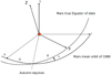 |
Fig. 1 Euler angles between the rotating body frame of Mars (axes XYZ) and the inertial frame associated with the mean orbit of Mars of 1980 (axes xyz, the x-axis is in the direction of the ascending node of Mars's orbit over the Earth ecliptic of epoch J2000). The X-axis of the BF is chosen as the prime meridian defined in the IAU convention (Archinal et al. 2018). The spin axis longitude ψ is measured from the x-axis to the autumn equinox, ϕ is measured from the equinox to the X-axis, and the obliquity, ε, is the angle from the z-axis to the Z-axis – or the inclination of the BF equator over the IF xy plane. |
2 Theory
Two different types of relativistic contributions exist which arise in the BCRS rotation model of Solar System bodies: (i) contributions that impact directly the rotation of the body and (ii) contributions arising from reference frame transformation. The first type of contributions concerns the ones that impacts the spin equation of motion such as the geodetic precession and nutations (Fukushima 1991; Eroshkin & Pashkevich 2007; Baland et al. 2020) and the Lense-Thirring and Thomas precessions (see Sect. 2.1). The second relativistic contributions come from the reference frame transformation between a local inertial frame that would be used to describe the local physics of the body and the BCRS used to analyze the data. The theory of reference frame transformation to first post-Newtonian order has been derived by Brumberg & Kopejkin (1989); Kopejkin (1988); Damour et al. (1991); Klioner & Voinov (1993) – and it has also been adopted in the IAU 2000 conventions, as in Soffel et al. (2003). Of prime importance for our purpose is the time transformation between a local reference frame and BCRS. In Sect. 2.2, we will present in details various contributions that arise in the time transformation and their impact in terms of the Mars rotation model.
2.1 Geodetic, Lense-Thirring, and Thomas precession effects
Within general relativity framework, the evolution of a spinning body is given, at the first post-Newtonian approximation, by a simple precession relation (see e.g., Barker & O'Connell 1970; Soffel et al. 2003; Poisson & Will 2014):
 (4)
(4)
In this equation, S denotes the spin angular momentum of Mars and Ω is the relativistic total precessional angular velocity, which is decomposed into three parts: Ω = Ωso + Ωss + ΩΤΡ. The term Ωso is called the spin-orbit precessional angular velocity, is the spin-spin precessional angular velocity, and ΩΤΡ is called the angular velocity of the Thomas precession. The spin-orbit and spin-spin components are also called the "geodetic precession" and the "Lense-Thirring precession," respectively.
When applying Eq. (4) to the description of the spin variations of Mars, we can keep the contribution of the Sun only in the relations of the spin-orbit and spin-spin precessional angular velocities, while the contribution of Phobos alone can be retained in the relation of the Thomas precession angular velocity. Thus, the expressions of the angular velocities are as follows:
 (5a)
(5a)
 (5b)
(5b)
 (5c)
(5c)
where x and x⊙ are the barycentric positions of Mars and of the Sun, respectively, and v and v⊙ represent their barycentric velocities. The vector Q is the non-geodesic acceleration whose expression can be derived from Eq. (6.30a) of Damour et al. (1991); hereafter, we only consider the dominant Newtonian contribution. In addition, M⊙ is the mass of the Sun, while S⊙ and ê⊙ denote the magnitude and direction of the Sun's spin angular momentum, respectively, c is the speed of light, and G is the universal gravitational constant.
Hereafter, we write ê⊙ = cos α⊙ cos δ⊙ êx + sin α⊙ cos δ⊙ êy + sin δ⊙ êz with α⊙ and δ⊙ as the right ascension and declination of the direction of the Sun's spin axis, respectively. Both are assumed to be fixed in the inertial frame associated with the mean orbit of Mars, namely (êx, êy, êz). We also consider that M/M⊙ ≪ 1, so that Mars follows an heliocentric orbit, namely ‖x⊙‖/‖x‖ ≪ 1, ‖v⊙‖/‖v‖ ≪ 1. We denote by êz the direction of the orbital angular momentum of Mars (assumed to be constant) and by êx the direction of the ascending node of Mars's orbit in the ecliptic; êy completes the triad such that (êx, êy, êz) is a direct orthogonal basis. After decomposing Eqs. (5a) and (5b) into this basis (the case of the Thomas precession is treated separately at the end of the section), we obtain the following relationships:
 (6a)
(6a)
 (6b)
(6b)


where a is the semi-major axis, e is the eccentricity, and f is the true anomaly for Mars. We neglected e in Ωss, as the Lense-Thirring effect obtained for a circular orbit is already very small (between three and four orders of magnitude smaller than the geodetic effect; for more, see below).
We now write the components of êx, êy, and êz in the coordinates of a rotating frame attached to Mars (êX, êY, êZ) and oriented with the Euler angles (ψ, ε, ϕ), with details given in Fig. 1:
 (8a)
(8a)
 (8b)
(8b)
 (8c)
(8c)
The precessional angular velocities Ωso and Ωss can also be written as function of the Euler angles such as:
 (9)
(9)
where a "dot" denotes a differentiation with respect to time.
By merging Eq. (9) with Eq. (6a), we obtain  , so that only the longitude angle ψ is affected by the geodetic effect
  . We proceed to a change of variable (from t to f):
 (10)
(10)
with dt/df being given by p3/2(GM⊙)−1/2(1 + e cos f)−2 for a Keplerian motion, where p = a(1 − e2) the semi-latus rectum of Mars's orbit. After substituting the expression of dt/df into the right-hand side of Eq. (10), the integration is immediate (see also Eq. (3) of Fukushima 1991) and leads to
 (11)
(11)
After using the equation of the center (see e.g., Murray & Dermott 2000) to express the true anomaly in term of the mean anomaly, l′, the expression for the spin axis longitude of Mars is given by:
 (12)
(12)
where the Jk(x) are the Bessel functions of first kind with k-index, and n is the Mars's mean motion which is given by Kepler third law of motion. The term which is directly proportional to Mars's mean anomaly describes a precession in longitude at a steady rate, while the other periodic terms represent the nutations in longitude. After making use of the numerical values given in Table 1, we find the following estimate reported here at third-order in eccentricity:
 (13)
(13)
Since the geodetic precession and nutations are small, the toy model based on the assumption of an elliptic Keplerian orbit is accurate enough for our purposes. The precession and annual terms are above the 0.1 mas threshold and must be included in a model for the longitude angle, ψ, as done, for instance, in Baland et al. (2020). The geodetic precession term is larger than the uncertainty on the determination of the precession rate (−7598.3 ± 2.1 mas yr−1, Le Maistre et al., in prep.) and is needed to avoid an error of about 0.1% in the determination of the polar moment of inertia. The geodetic annual term, with its amplitude of 0.6 mas, does not depend on the properties of Mars's interior and has to be removed from any determination of the annual nutation term before any interpretation in terms the of core radius for instance.
By merging Eq. (9) with Eq. (6b), we obtain the equation of motion for the Euler angles related to the Lense-Thirring effect:
 (14a)
(14a)
 (14b)
(14b)
 (14c)
(14c)
After integration (we considered the angles ψ and ε as constant in the right-hand sides of the equations, and therefore denote them with a subscript "0" in the following), the solution for each angle will be the sum of a linear term and of a periodic term at the semi-annual period. After making use of numerical values given in Table 1, we find the following estimate:
 (15a)
(15a)
 (15b)
(15b)
 (15c)
(15c)
We actually see that the spin-spin contribution is well below the 0.1 mas precision and can therefore be safely neglected, as compared to the spin-orbit contribution.
While considering the spin of Mars as an accelerated gyroscope, we also consider the Thomas precession ΩΤΡ contribution within the total relativistic angular precessional velocity Ω (see e.g., Eq. (25) of Soffel et al. 2003). As shown in Eq. (5c), this term is proportional to the acceleration that characterizes the deviation of the actual worldline of the planet from a geodesic, which comes mainly from the coupling of higher order multipole moments of Mars to the external tidal gravitational fields. The Thomas precession scales as ΩΤΡ = ‖ΩTP‖ ∝ Q‖v‖/c2, with Q = ‖Q‖ ∝ J2R2GMp/‖x − xp‖4; here, J2 and R are respectively the quadrupole moment and the equatorial radius of Mars, while Mp and xp are the mass and the barycentric position of the external body, respectively. For the Earth, the dominant contribution to Thomas precession comes from the Moon. Here, for Mars, Phobos plays the dominant role. The absolute value of Q due to the action of Phobos is on the order of 10−12 m s−2, meaning that ΩΤΡ ~ 10−6 μas yr−1 (against 105 μas yr−1 and 10−1 μas yr−1 for Ωso and Ωss, respectively). The contribution of Thomas precession to the variations in Euler angles is therefore smaller than the already negligible contribution of the Lense-Thirring precession.
Parameter values used for computing the relativistic contributions to the Mars BCRS rotation model, in the frame of analytical and toy model developments of Sects. 2.2 and 3.1, where the orbit of the planets are assumed to be Keplerian.
2.2 Time coordinate transformation and impact on Mars rotation modeling
We denote, using τ, the local time (or proper time) related to the central body (i.e., Mars) and, using t, the barycentric dynamical time (TDB), which is related to the BCRS and used to analyze the data at Mars. The local model of rotation describes the rotation of the body in terms of local physics such as the atmosphere and surface dynamics. This model is typically expressed as a function of the local time, τ. For example, for a uniformly rotating body, we have  . As a consequence, when expressed in BCRS, the rotation model will be impacted by the τ − t time transformation. In Sect. 2.2.1, we present the theory related to the time transformation, while in Sect. 2.2.2, we show how this time transformation impacts the modeling of Mars's rotation when expressed in BCRS.
2.2.1 Time coordinate transformation
The t of TDB is a rescaled version of barycentric coordinate time (TCB). The link between TDB and TCB is defined by the recommendation B3 of IAU2006, which reads:
 (16)
(16)
where LB = 1.550519768 × 10⁻⁸; as in Eq. (10.3) from Petit et al. (2010).
The proper time related to a local frame co-moving with Mars (the Martian equivalent to geocentric coordinate time, or TCG) is denoted here as τ. For a small orbital velocity (υ ≪ c) and a weak gravitational field (r ≫ GM/c2), the relationship between TDB and Mars's proper time τ at first post-Newtonian order is given by (see, e.g., Soffel et al. 2003; Petit et al. 2010)
![$\matrix{ {{{{\rm{d}}\tau } \over {{\rm{d}}t}} - 1 = {{\left[ {{{{\rm{d}}\tau } \over {{\rm{d}}t}}} \right]}_{{\rm{GR}}}} = {{{L_{\rm{B}}}} \over {1 - {L_{\rm{B}}}}} - {1 \over {{c^2}}}{1 \over {1 - {L_{\rm{B}}}}}\left( {{{{\upsilon ^2}} \over 2} + \omega } \right)} \hfill \cr {\quad \quad \quad \quad + {1 \over {{c^4}}}{1 \over {1 - {L_{\rm{B}}}}}\left( { - {{{\upsilon ^4}} \over 8} - {3 \over 2}{\upsilon ^2}{\omega ^2} + 4\bf{\rm v} \cdot \bf{\rm w} + {1 \over 2}{\omega ^2} + \Delta } \right),} \hfill \cr } $](/articles/aa/full_html/2023/02/aa44420-22/aa44420-22-eq35.png) (17)
(17)
where v is Mars's barycentric velocity. The potential, w, is the Newtonian potential at the location of Mars:
 (18)
(18)
where rA = ‖x − xA‖ with x the barycentric position of Mars and xA is the position of the body A, and where the sum includes the Sun and all planets, R⊙ is the Sun's equatorial radius, ê⊙ is the unit vector defining the Sun's spin axis, and  is the Sun's quadrupolar moment of the mass distribution. The norm of the barycentric distance between Mars and the Sun is denoted r⊙ = ‖x − x⊙‖. In addition, w is the vector potential defined by:
 (19)
(19)

where aA is the Newtonian point-mass acceleration of body A, namely,
 (21)
(21)
We can write the result from the integration of Eq. (17), the relationship between TDB and Mars's propertime, τ, as
![$\tau = t + \left[ {\tau - t} \right]{\rm{GR,}}$](/articles/aa/full_html/2023/02/aa44420-22/aa44420-22-eq41.png) (22)
(22)
where [τ−t]GR includes the various relativistic corrections. Typically the relative amplitude of [τ − t]GR is of the order of GM⊙/c2a ~ 10−8, where a is Mars's semi-major axis. In the following, we show how these relativistic corrections impact the data analysis related to the rotation of Mars when analyzed using TDB.
2.2.2 Impact on rotation modeling for Mars
We now explore how the time transformation developed above can impact Mars rotation modeling in BCRS. We first consider a rotation model expressed in Mars's local reference frame. Such a model includes a uniform rotation and periodic terms, that is,
 (23)
(23)
On the other hand, one needs a similar modeling expressed in terms of TDB in order to perform the data analysis. Using Eq. (22), this modeling is given as:
![$\matrix{ {\phi \left( t \right) = {\phi _{{\rm{local}}}}\left( {\tau \left( t \right)} \right) = {\phi _0} + \dot \phi _0^{{\rm{local}}}t - {\psi _{{\rm{nut}}}}\cos {\varepsilon _0}} \hfill \cr {\quad \quad \quad + \sum\limits_{j = 1}^4 {\left( {{\phi _{cj}}\cos \,jl' + {\phi _{sj}}\sin \,jl'} \right) + {{\left[ \phi \right]}_{{\rm{GR}}}}\left( t \right),} } \hfill \cr } $](/articles/aa/full_html/2023/02/aa44420-22/aa44420-22-eq43.png) (24)
(24)
![${\left[ \phi \right]_{{\rm{GR}}}}\left( t \right) = \dot \phi _0^{{\rm{local}}}{\left[ {\tau - t} \right]_{{\rm{GR}}}}.$](/articles/aa/full_html/2023/02/aa44420-22/aa44420-22-eq44.png)
When analyzing data from orbiting spacecraft or surface landers, the timescale used in the data reduction is TDB, so that the model for Mars rotation needs to include the relativistic contributions, as presented above. In the following section, we study, both numerically and analytically, various contributions that impact the [τ − t]GR relationship and their impact on Mars's rotation angle ϕ. We go on to propose a new modeling process that improves upon the one currently used in various analyses.
Additional relativistic corrections in longitude and obliquity can be computed similarly as for the rotation angle, by replacing the rotation rate in Eq. (25) by the precession rate in longitude and in obliquity. However, as those rates (−7598.3 mas yr−1 and −7.9 mas yr−1, respectively, see Le Maistre et al., in prep.) are very small compared to the rotation rate, the associated relativistic corrections are negligible.
3 Impact of the time transformation on Mars rotation modeling
In this section, we study the various contributions to the [τ−t]GR relationship that arise from the integration of Eq. (17) and their corresponding impacts on the Mars BCRS rotation model through Eq. (25). In order to cross-check and validate our results, we developed three independent approaches.
The first approach consists of developing a simple toy model to analytically integrate Eq. (17). This provides a good physical intuition with regard to the various terms obtained and the process is relatively pedagogical. The second approach consists of numerically integrating Eq. (17) using the DE440 planetary ephemerides (Park et al. 2021) provided by the NAIF-SPICE software (Acton 1996; Acton et al. 2018). In a subsequent step, analytical series consisting in various harmonic terms are fitted to the result of the numerical integration. This procedure is similar to the one developed to produce the Ephemeris Time (ET) for Earth. For details, we refer to Fukushima (1995, 2010), Irwin & Fukushima (1999), and Harada & Fukushima (2003).
The third approach we developed consists of using a series for the barycentric position and distance of planets to obtain a subsequent series for the relativistic part of the rotation angle. We use the analytical planetary theory VSOP87 (Bretagnon & Francou 1988), derived from the DE200 planetary ephemerides (Standish 1982). Using the VSOP87 series, we analytically integrate Eq. (17) and identify the harmonics with the largest contribution to the [τ−t]GR relationship. We purposely used VSOP87 in this instance, instead of the more recent versions of VSOP theories that are not suited for our purpose. VSOP2000 (Moisson & Bretagnon 2001) provides a series only for the heliocentric positions (not the barycentric positions), whereas VSOP2013 (Simon et al. 2013), derived from the INPOP planetary ephemerides (Fienga et al. 2011; Bernus et al. 2019, 2022), is based on Tchebychev polynomials (and not on a series). We go on to show that the error introduced by using the older (and therefore less accurate) VSOP87 theory is negligible for our purpose, as the solutions of the second and third approaches are consistent to the 0.1 mas level.
The advantages to considering the last two approaches are rooted in the fact that we can cross-check our results and estimate the uncertainties in our derived modeling coming from numerical integration, differences between the DE and INPOP ephemerides, and so on.
In the remainder of this section, we consider the various contributions from Eq. (17): the 1/c2 contribution coming from the two-body problem, contribution related to the motion of the Sun with respect to the Solar System barycenter (SSB), contribution from the LB constant, direct contribution from other planets, and higher order contributions (i.e., the 1/c4 terms and the Sun's  ).
).
3.1 Simple analytical solution (toy model)
3.1.1 The 1/c2 contribution coming from the Sun considering a Keplerian motion
We first consider the main contribution to the relation between τ and TDB, which is the 1/c2 contribution from the Sun in a two-body (or Keplerian) problem.
The evolution of proper time with respect to coordinate time is given by:
![${{{\rm{d}}\tau } \over {{\rm{d}}t}} - 1 = {\left[ {{{{\rm{d}}\tau } \over {{\rm{dt}}}}} \right]_{{\rm{2body}}}} = {{{L_{\rm{B}}}} \over {1 - {L_{\rm{B}}}}} - {1 \over {1 - {L_{\rm{B}}}}}{{\upsilon _{M \odot }^2} \over {2{c^2}}} - {1 \over {1 - {L_{\rm{B}}}}}{{G{M_ \odot }} \over {{r_{M \odot }}{c^2}}},$](/articles/aa/full_html/2023/02/aa44420-22/aa44420-22-eq46.png) (26)
(26)
where rM⊙ is the distance between the Sun and Mars and vM⊙ is the norm of their relative velocity. This expression can be integrated exactly assuming a perfect Keplerian motion, as in, for instance, Moyer (1981):
![$\matrix{ {{{\left[ {\tau - t} \right]}_{{\rm{2body}}}}} \hfill & { = {\rm{cst}} + {{{L_{\rm{B}}}} \over {1 - {L_{\rm{B}}}}}t - {1 \over {1 - {L_{\rm{B}}}}}{{n{a^2}} \over {2{c^2}}}\left( {4E - nt} \right),} \hfill \cr {} \hfill & { = {\rm{cst}} + {{{L_{\rm{B}}}} \over {1 - {L_{\rm{B}}}}}t - {1 \over {1 - {L_{\rm{B}}}}}{{n{a^2}} \over {{c^2}}}\left( {2e\sin \,E + {3 \over 2}l'} \right),} \hfill \cr } $](/articles/aa/full_html/2023/02/aa44420-22/aa44420-22-eq47.png) (27)
(27)
where n is the mean motion, a the semi-major axis, E is the eccentric anomaly, and l′ is the mean anomaly. A low eccentricity expansion leads to:
![$\matrix{ {{{\left[ {\tau - t} \right]}_{{\rm{2body}}}} = } \hfill & {{\rm{cst}} + {1 \over {1 - {L_{\rm{B}}}}}\left( {{L_{\rm{B}}} - {{3{n^2}{a^2}} \over {2{c^2}}}} \right)t} \hfill \cr {} \hfill & { - {{n{a^2}} \over {{c^2}\left( {1 - {L_{\rm{B}}}} \right)}}\left( {2e - {{{e^3}} \over 4}} \right)\sin l'} \hfill \cr {} \hfill & { - {{n{a^2}} \over {{c^2}\left( {1 - {L_{\rm{B}}}} \right)}}\left( {{e^2} - {{{e^4}} \over 3}} \right)\sin 2l'} \hfill \cr {} \hfill & { - {{3n{a^2}} \over {4{c^2}\left( {1 - {L_{\rm{B}}}} \right)}}{e^3}\sin 3l'} \hfill \cr {} \hfill & { - {{2n{a^2}} \over {3{c^2}\left( {1 - {L_{\rm{B}}}} \right)}}{e^4}\sin 4l' + ...,} \hfill \cr }$](/articles/aa/full_html/2023/02/aa44420-22/aa44420-22-eq48.png) (28)
(28)
which includes a linear drift and oscillations at frequencies multiple of the orbital frequency. The linear drift includes a contribution from the rescaling between TCB and TDB (i.e., the contribution from LB) of 1.55 × 10⁻⁸ and a contribution of −9.72 × 10⁻⁹ from the Sun (using Mars's orbital parameters from Table 1). The total linear drift coefficient is 5.79 × 10⁻⁹. The amplitudes of the harmonics terms are: −11.419 ms for the term at orbital period, −532.3 μs for the term at twice the orbital period, −37.4 μs for the term at three times the orbital period, and −3.1 μs for the term at four times the orbital period. We note that the 1/(1 − LB) coefficient impacts these amplitude only at the relative level of 10−8.
The impact on Mars's rotation is obtained from Eq. (24). First of all, it is important to notice that the  estimated from a data analysis performed in BCRS is actually:
 (29)
(29)
where  is the proper Mars rotation rate. Using the measured value of
  from Table 1, we can find:
 (30)
(30)
such that  is 2°.03 × 10−6 day−1 (or 7.3117 mas day−1). This quantity is two orders of magnitude larger than the current uncertainty in the Mars rotation rate estimate and thus must be removed for any geophysical interpretation of the latter (
 in Eq. (2) must be replaced by
  ).
).
The 2-body contribution from the transformation between τ and t to the Mars rotation model in BCRS, including the linear term and the four largest periodic terms, is
![$\matrix{ {{{\left[ \phi \right]}_{2{\rm{body}}}}} \hfill & = \hfill & {\dot \phi _0^{{\rm{local}}}{{\left[ {\tau - t} \right]}_{{\rm{GR}}}} = {{\dot \phi }_{{\rm{GR}}}}t + \sum\limits_j {{\phi _{rj}}\sin j\,l',} } \hfill \cr {} \hfill & = \hfill & {2^\circ .03 \times {{10}^{ - 6}}{\rm{da}}{{\rm{y}}^{ - 1}} \times t} \hfill \cr {} \hfill & {} \hfill & { - 166.950\,{\rm{mas}}\sin l' - 7.782\,{\rm{mas}}\sin 2l'} \hfill \cr {} \hfill & {} \hfill & { - 0.547\,{\rm{mas}}\sin 3l' - 0.045\,{\rm{mas}}\sin 4l'.} \hfill \cr }$](/articles/aa/full_html/2023/02/aa44420-22/aa44420-22-eq57.png) (31)
(31)
These values will be refined in the further subsections considering a more accurate modeling of Mars's trajectory. Nevertheless, the Keplerian modeling presented here is sufficient to get an estimate of the order of magnitude of the impact of the time transformation on the rotation of Mars.
3.1.2 Contribution related to the motion of the Sun with respect to the Solar System barycenter
The two-body problem calculation performed in the previous section considers one test mass orbiting one massive body, assuming that the coordinate time TDB is the one related to a coordinate system where the massive body is at rest at the origin. For BCRS, this is not the case: the Sun is not at rest and not located at the origin of the coordinate system that is defined as the SSB. Therefore, when we are interested in computing the evolution of Mars proper time with respect to TDB, we should use:
 (32)
(32)
where vM is Mars's velocity with respect to the SSB and rM⊙ is the distance between Mars and the Sun. The only difference with respect to Eq. (26) relies on the velocity expressed relative to the SSB and not to the Sun. A simple calculation using vM = vM⊙ + v⊙, where vM⊙ is the velocity of Mars with respect to the Sun and v⊙ is the Sun velocity with respect to the SSB, shows that there is an additional contribution to the evolution of Mars proper time due to the velocity of the Sun with respect to the SSB. This additional contribution is given by:
![${\left[ {{{d\tau } \over {dt}}} \right]_{{\rm{SSB}}}} = - {1 \over {1 - {L_{\rm{B}}}}}{{{\upsilon _ \odot } \cdot {{\bf{v}}_{{\rm{M}} \odot }}} \over {{c^2}}} - {1 \over {1 - {L_{\rm{B}}}}}{{\upsilon _ \odot ^2} \over {2{c^2}}} \approx - {{{{\bf{v}}_ \odot } \cdot {{\bf{v}}_{{\rm{M}} \odot }}} \over {{c^{\rm{2}}}}}.$](/articles/aa/full_html/2023/02/aa44420-22/aa44420-22-eq59.png) (33)
(33)
To first order, the motion of the Sun with respect to the SSB is due to its gravitational interaction with Jupiter. If we take a simple toy model and consider that the motion of the Sun with respect to the SSB is due to Jupiter only and assuming Jupiter's orbit to be circular around the Sun, then the Sun's velocity is given by  (sin nJt, − cos nJt, 0), where aJ is Jupiter's semi-major axis and nJ its mean motion. To a first approximation, we can also consider the orbital motion of Mars to be circular; then, Eq. (33) can be integrated analytically:
![${\left[ {\tau - t} \right]_{{\rm{SSB}}}} \approx {{a{a_{\rm{J}}}} \over {{c^2}}}{{n{n_{\rm{J}}}} \over {n - {n_{\rm{J}}}}}{{{M_{\rm{J}}}} \over {{M_ \odot }}}\sin \left( {\left( {n - {n_{\rm{J}}}} \right)t + \delta } \right),$](/articles/aa/full_html/2023/02/aa44420-22/aa44420-22-eq61.png) (34)
(34)
where a is Mars's semi-major axis, n its mean motion, and δ the phase difference between the two planets, assuming co-planar motion. The velocity of the Sun with respect to the SSB therefore induces an additional modulation to the transformation from τ to the TDB. The period of this modulation is the Mars-Jupiter synodic orbital period, namely, 2.235 yr, and its amplitude is 37.59 μs.
Using Eq. (25), this modulation impacts the BCRS Mars rotation modeling and induces a modulation of amplitude of 0.55 mas at the Mars-Jupiter synodic orbital period. A similar calculation considering Saturn leads to a harmonic term of period of 2 yr with an amplitude of 0.11 mas. The other planets induce periodic terms with amplitudes ≲0.01 mas. This can be seen as an indirect effect of the other planets of the Solar System on Mars propertime since it comes from the impact of other planets on the SSB velocity. The direct effect will be computed below.
3.1.3 Direct contribution from other planets
As can be noticed from Eq. (17), the gravitational potential from the other planets will also impact the evolution of Mars proper time. To first order, the impact from the planets gravitational potential is governed by
![${\left[ {{{d\tau } \over {dt}}} \right]_{\rm{P}}} = - {1 \over {1 - {L_{\rm{B}}}}}{{G{M_{\rm{P}}}} \over {{c^2}{r_{{\rm{M}}P}}}},$](/articles/aa/full_html/2023/02/aa44420-22/aa44420-22-eq62.png) (35)
(35)
where rMP = ‖xM − xP‖ is the distance between Mars and a planet P.
A simple toy model considering both Mars and the planet to be orbiting on coplanar circular orbits shows that, to first order, the integration of the previous equation leads to a linear drift whose linear coefficients is given by  and to an harmonic signal at the planet-Mars synodic orbital period and of amplitude of
  , where aP and nP are the semi-major axis and mean motion of the planet P. This calculation is valid only to first order in
  and neglecting LB. Other harmonics can be identified at higher orders and for non-zero eccentricities, in particular an oscillation at the orbital period of the planet (see Sect. 3.3).
For each planet P, these contributions to the τ to TDB transformation will impact Mars's BCRS rotation modeling through Eq. (25), that is to say, it will produce one term with linear rate  and one harmonic synodic term. For Jupiter,
  (or −0.00220 mas day−1). For Saturn,
  (or −0.00037 mas day−1). The synodic terms associated to Jupiter and Saturn have amplitudes of 0.077 mas and 0.007 mas, respectively. The other planets induce synodic terms with amplitudes ≲0.001 mas. Although the direct synodic terms associated to Jupiter and Saturn have small amplitudes, they cannot be neglected as they combine with the indirect synodic terms obtained in the previous subsection. The total synodic terms related to Jupiter and Saturn have 0.47 mas and 0.10 mas of amplitude, respectively, as the direct and indirect terms are out of phase to each other. The sum of the direct and indirect effect of the planets will be refined in the further subsections considering a more accurate modeling of each planet’s trajectory.
Similarly as for the effect of the planets, it is possible to build a toy model for the direct effect of Phobos and Deimos, and of Ceres, the largest body of the asteroid belt. However, given their small mass, the associated relativistic corrections can be neglected.
3.2 Numerical solution using the DE planetary ephemerides
In this section, we present the result of a numerical integration of Eq. (17) using the DE440 planetary ephemerides (Park et al. 2021) provided by the NAIF-SPICE software (Acton 1996; Acton et al. 2018). The integration was performed starting from J2000 and lasting 30 yr backward and forward. In a second step, analytical series consisting of various harmonic terms were fitted to the result of the numerical integration. This procedure is similar to the one developed to produce the Time Ephemeris for Earth (see Fukushima 1995, 2010; Irwin & Fukushima 1999; Harada & Fukushima 2003).
3.2.1 First-order contributions
In this section, we consider the leading contributions from Eq. (17), namely, the 1/c2 contributions from the Sun, the various planets, and from LB. This integration therefore includes all the effects presented in the previous section. We numerically integrate Eq. (17) and transform the evolution of τ − t into an estimate of the evolution of ϕ through Eq. (25). We then fit the expression
![${\left[ \phi \right]_{{\rm{GR}}}}\left( t \right) = {{\dot \phi }_{{\rm{GR}}}}t + \sum\limits_j {\left( {{C_j}\cos {f_j}t + {S_j}\sin {f_j}t} \right)}$](/articles/aa/full_html/2023/02/aa44420-22/aa44420-22-eq69.png) (36)
(36)
to the numerically integrated evolution of [ϕ]GR(t). The values of the various coefficients  , Cj, and Sj are obtained using a standard linear least-squares fit. Motivated by the toy model presented in the previous section, the angular frequencies, fj, included in the fit are chosen as linear combinations of the planets mean motion. We identify the relevant frequencies by (iteratively) searching for the largest peaks in the Fourier transform of the numerically integrated [ϕ]GR(t) time series. The fitted coefficients are then transform to obtain the following expression:
![${\left[ \phi \right]_{{\rm{GR}}}}\left( t \right) = {{\dot \phi }_{{\rm{GR}}}}t + \sum\limits_j {{A_j}\sin \left( {{f_j}t + {\varphi _j}} \right).}$](/articles/aa/full_html/2023/02/aa44420-22/aa44420-22-eq71.png) (37)
(37)
The estimated linear term is  (or 7.308758 mas day−1), while the amplitude and phase of the harmonic terms are given in Table 2. We searched for terms with amplitude down to 0.04 mas, covering the amplitude range considered in Eq. (31) for the terms at the harmonics of the Martian orbital period. For these terms, the estimated solution is in good agreement with the solution of the toy model (difference <0.005 mas), but differs significantly with respect to Eq. (21) of Yoder & Standish (1997), recalled in Eq. (3), with up to 9 mas, or 5% in annual amplitude. The differences are mainly likely due to truncation errors in the parameters values used by Yoder & Standish (1997). The estimated terms at the Mars-Jupiter and Mars-Saturn synodic periods are 0.10 mas and 0.005 mas larger than obtained with the toy model, as a result of the assumption of circular planetary orbits therein. We also find one term at the orbital period of Jupiter with an amplitude of about 0.04 mas, related to the direct effect of the planet, and three others terms at different periods with amplitude ranging between 0.06 mas and 0.08 mas, mainly due to the indirect effect of the Earth and of Jupiter of the orbit of Mars.
The residuals between the numerical integration and the fitted harmonics decomposition is presented in Fig. 2 and remains below 0.15 mas. Formal uncertainties are not relevant quantities to characterize the errors of the fit as they do not directly rely on any observations (no data points). Instead, we use another method described in Sect. 3.3.2 to compute the accuracy of the estimated coefficients, which is equal to ~0.01 mas, on the main terms.
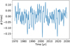 |
Fig. 2 Difference between the [ϕ]GR(t) obtained by numerically integrating Eq. (17), using the DE440 planetary ephemerides and using Eq. (25) and the fitted series from Eq. (37). This curve provides an estimate of the accuracy of the fitted analytical model provided by the coefficients from Table 2. |
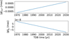 |
Fig. 3 Impact of the 1/c4 term from Eq. (17) on the BCRS modeling of Mars’s rotation (top). Impact of the Sun quadrupole moment |

3.2.2 Higher-order contributions
In this section, we consider the 1/c4 contribution appearing in Eq. (17) and the contribution from the Sun’s quadrupole moment,  . Their impact on the BCRS modeling of Mars’s rotation is presented in Fig. 3 and is on the order of μ as for the 1/c4 term and on the order of 10 nas for the
  . Both these contributions can safely be neglected.
3.3 Series solution using VSOP ephemerides
In this section, we present the results of a semi-analytical approach based on series for the barycentric position and distance of planets as provided by the analytical planetary theory VSOP87 (Bretagnon & Francou 1988). We integrate Eq. (17), neglecting the 1/c4 and Sun’s  contributions, identify the harmonics with the largest contribution to the τ − t relationship, and estimate the evolution of ϕ through Eq. (25). In a second step, we numerically assess the accuracy of the semi-analytical solution.
3.3.1 Semi-analytical solution
In VSOP87, the barycentric Cartesian coordinates (X, Y, Z) and distance r of the planets to the Sun are written as series of the form:
 (38a)
(38a)
 (38b)
(38b)
 (38c)
(38c)
where Cα,j and Sα,j are amplitudes and T is the time measured in thousands of Julian years from J2000. φj are linear combinations of fundamental arguments, including the mean longitudes of Saturn (Sa), Jupiter (Ju), Mars (Ma), and the Earth (Te); we refer to Table 2 of (Bretagnon & Francou 1988):
 (39a)
(39a)
 (39b)
(39b)
 (39c)
(39c)
 (39d)
(39d)
The power α is an integer in-between 0 and 5. For α = 0, the series are periodic. For α ≥ 1, the series are pseudo-periodic (Poisson series).
The solution for [ϕ]GR(t) is firstly written as:
![${\left[ \phi \right]_{{\rm{GR}}}}\left( t \right){\rm{ = }}{{\dot \phi }_{{\rm{GR}}}} \times t + \sum\limits_j {\left( {\Delta \phi _j^c\cos {\varphi _j} + \Delta \phi _j^s\sin {\varphi _j}} \right),} $](/articles/aa/full_html/2023/02/aa44420-22/aa44420-22-eq84.png) (40a)
(40a)
 (40b)
(40b)
with  the amplitudes of the periodic and Poisson series. In the first place, the fundamental arguments of the series will be the same as the VSOP87 arguments, by construction, because the series for υ2, the squared Mars barycentric velocity, is directly obtained as the squared norm of the time derivative of the position vector of Mars (X, Y, Z), while the series for 1/r⊙ is obtained starting with the VSOP series for r⊙ and following Eq. (61) of Baland et al. (2020). The distance rP between Mars and another planet varies greatly with time, and as a result, it is difficult to express as convergent series for 1/rP starting from the VSOP series for the Cartesian coordinates. We therefore assume that the orbits of Mars and of the other planets are Keplerian and coplanar and use the mean orbital elements of Simon et al. (2013). We adapted the procedure described in Sect. 4.3.3 of Baland et al. (2020) to obtain a series for
  to the case of 1/rP. This can be seen as extension of the toy model presented in Sect. 3.1.3 to higher orders in eccentricities and in
  and, as a result, we go on to identify more harmonics and obtain different amplitudes.
Then, for consistency with the usual form of [ϕ]GR(t), expressed with the mean anomaly, l′, of Mars as the argument (see Eq. (3)), we change the fundamental arguments, using the mean anomalies of the planets
 (41a)
(41a)
 (41b)
(41b)
 (41c)
(41c)
 (41d)
(41d)
instead of their mean longitudes. We express [ϕ]GR(t) correct up to the first order in the rates of the pericenter longitudes ϖ of the planets, creating a second Poisson series, to add to the first Poisson series coming directly from VSOP ephemerides, and which is not affected by the argument change, at first order. Both Poisson series are similar, but with opposite amplitudes, and therefore they almost cancel each other (the sum of the two series is smaller than 0.05 mas on the interval ±30 yr around J2000 and significant Poisson terms were not found in the fit of the numerical solution). As a result, we omitted Poisson series in the following.
Finally, the periodic series in [ϕ]GR(t) is written in a pure Sine form, convenient for the purposes of application:
![${\left[ \phi \right]_{{\rm{GR}}}}\left( t \right) = {{\dot \phi }_{{\rm{GR}}}}t + \sum\limits_j {\phi _j^r\sin \left( {{f_j}t + \varphi _j^0} \right),}$](/articles/aa/full_html/2023/02/aa44420-22/aa44420-22-eq93.png) (42)
(42)
with  the amplitudes and
  a phase (different from that of Eq. (40a)); fj represents the linear combination of the rate of the mean anomalies of Eq. (41).
For the constant rate, we find  mas day−1, in agreement with the sum of the respective contributions from LB, from the Sun and from each planet, as obtained with the fit of the numerical solution. The periodic terms, with amplitudes down to 0.04 mas, are presented in Table 3. We find the same ten periodic terms as with the fit of the numerical solution of Table 2, but also one additional term, at the orbital period of Saturn (~30 yr) and with an amplitude of 0.043 mas. We did not find this term with the fit because of its long period and of its small amplitude.
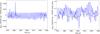 |
Fig. 4 Difference between the solutions for [ϕ]GR(t) obtained using VSOP87 and DE440 ephemerides via numerical integrations (left). Difference between the numerical integration and the semi-analytical solution using VSOP87, with only the 11 terms of Table 3 in blue, with all terms in black (right). |
3.3.2 Accuracy of the semi-analytical solution
The difference between the numerical integrations of [ϕ]GR(t) performed using the recent DE440 and the older VSOP87 ephemerides is presented in the left panel of Fig. 4, and it remains below 0.003 mas, indicating that using the VSOP87 theory should not be a cause of major errors.
The different steps of the computational procedure to obtain the semi-analytical solution of Eq. (40a) introduce residuals smaller than 0.05 mas when all the terms of the periodic series are considered, and smaller than 0.2 mas when only the 11 largest terms of the series are considered (see right panel of Fig. 4). This is in agreement with the residuals of the fitted solution to the numerical integration based DE440 ephemerides, which includes the ten periodic terms of Table 2 (see Fig. 2).
The amplitudes and phases of the fitted (Table 2) and semi-analytical (Table 3) solutions are in good agreement to each other (see also Fig. 5, where the difference remains below 0.06 mas). The differences give a sense of the modeling uncertainties: for instance, 0.01 mas (0.005%) in annual amplitude or 0.01 mas (0.9%) on the Mars-Jupiter synodic term. Both solutions or an averaged solution can be used for the purposes of application.
4 Signatures in the Doppler observable
As shown in the previous sections, the relativistic variations in Mars rotation and orientation mainly affect the angles ψ and ϕ. Using analytic expressions, we characterize in this section the signature of these variations in the Doppler observable of a Martian lander communicating directly with the Earth.
Numerical applications are provided for the specific case of RISE (Rotation and Interior Structure Experiment), the radio-science experiment of the NASA InSight mission (Folkner et al. 2018). The level of the signatures and their temporal behavior are compared to the noise level and non-relativistic signatures, respectively.
We note  as a variation in the precession, δ(ψnut) a variation in the nutation in longitude, and δϕ a variation (linear and/or periodic) in the rotation angle ϕ, excluding the nutation term ψnut cos ε0 (see Eqs. (1) and (2)). These three notations can be used to represent any kind of variations in ψ and ϕ, including the relativistic ones. Considering that #3, δ(ψnut), and δϕ are small quantities, their signature in the observable can be written to the first order as (Yseboodt et al. 2017):
 (43a)
(43a)
 (43b)
(43b)
 (43c)
(43c)
with θ as the lander latitude, R the radius of Mars, Ω the rotation rate, and δE the Earth declination relative to Mars’s equator. Each of these Doppler variations has a diurnal modulation via, HE, the Earth hour angle seen from Mars. The observable variations defined in Eq. (43) are Doppler shift expressed as the variation of the velocity along the line of sight (LOS). For a round-trip (two-way) radio link, the conversion factor between the LOS velocity and the Doppler observable is 2ft/c, with ft as the carrier downlink frequency. In the case of RISE (but also of LaRa, a radio transponder ready to fly to Mars, see Dehant et al. 2020), ft ≃ 8.4 GHz, which is in the X frequency band.
The signature of [ϕ]GR(t) (linear and/or periodic terms) is computed using Eq. (43c). The signature of the geodetic precession in longitude is obtained using Eq. (43a) and that of the geodetic nutation in longitude is computed with Eq. (43b). Precession and nutation signatures differ from each other because ψnut also affects the angle ϕ, while  does not (see Eqs. (1) and (2)).
The periodic variations in ϕ(t) induced by the seasonal atmosphere and surface dynamics (see, e.g., Konopliv et al. 2020) and by the time coordinates transformation altogether result in a maximum angular displacement of the lander of ~670 mas as seen from the center of Mars (1 mas corresponds to a displacement of 1.6 cm at the surface of Mars). For a lander located at the InSight landing site (i.e., Elysium Planitia: 4.5°N, 135.62°E, −2.6 km altitude), such an angular displacement induces a Doppler shift in the RISE measurements of ≲0.56 mm s−1 (see Fig. 2 of Yseboodt et al. 2017 or Table 4). A fourth of this Doppler signal, computed at the RISE tracking data-timing using the RISE frequency, comes from the relativistic periodic variations (see Fig. 6a and extra information in Table 4).
The combination of seasonal variations in Euler angles and of diurnal trend in the hour angle produces symmetrical envelopes with respect to zero in the Doppler signature, as seen in Figs. 6 and 7. Because of the repeatability in the RISE observation timing imposed by its fixed and directional antennas, the data points cover a limited part of these diurnal cycles.
The ~10 mas difference between the periodic terms of our solution for [ϕ]GR and that first estimated by Yoder & Standish (1997, see Eq. (3) and Sect. 3.2.1) has a Doppler signature lower than 0.007 mm s−1, which is smaller than the RISE noise level (1.1 mHz at 60 s integration time, corresponding to 0.02 mm s−1) and smaller than the liquid core signature (~0.01 mm s−1, Le Maistre et al., in prep). However, a precise solution for the Mars rotation angles (at the level of 1 mas or smaller) is needed to correctly interpret the measured periodic variations in terms of atmospheric constraints.
The signature in the Doppler of the relativistic linear term of 7.3 mas day−1 (see Eq. (46c)) is very large (up to 49 mm s−1), as shown in Fig. 6b. This pronounced signal with a linear increase that is barely visible in the plot occurs because it has a linear dependence on the time of the observations (2018–2022 for InSight) relative to the chosen reference epoch (here, J2000).
The signature of the geodetic nutation in longitude in the Doppler observable (shown in Fig. 7a) is very small (≤ 0.12 µm s−1), while that of the geodetic precession (linear term in Eq. (13)) is two to three orders of magnitude larger (up to 0.03 mm s−1), as shown in Fig. 7b, where the signature of the linear plus periodic geodetic terms is plotted (see Eq. (13)). Similarly as for the relativistic linear term in the rotation angle, the stronger signature of the geodetic linear term in longitude for Mars (6.75 mas yr−1) results from the linear dependency to the time past from the chosen origin of time (i.e., ~150 mas in 2020 for a reference epoch at J2000).
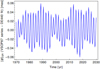 |
Fig. 5 Difference between the [ϕ]GR(t) of the semi-analytical solution using VSOP87 (with only the 11 terms of Table 3) and the fit of the numerical integration with DE440 ephemerides. |
5 Application to other planets
Mars has been extensively explored, but the rotation of other bodies of the Solar System is also subject to investigations. Here, we provide an estimate of the main terms of the relativistic correction in longitude, ψ, and rotation, ϕ, to include in the rotation model of our neighboring planets. For each planet, we first estimated the geodetic precession and nutation in longitude. Then we estimated the linear and periodic changes in rotation, considering (1) the Sun’s contribution with regard to a planet on a Keplerian orbit, (2) the contribution related to the Sun motion with respect to the SSB, and (3) the direct contribution from the other planets.
5.1 Geodetic precession and nutations
For any planet, the spin–orbit angular velocity Ωso of Eq. (5a) is proportional to x × v and therefore perpendicular to the orbital plane (see also Eq. (6a)). As a result, if a planet moves on a Keplerian orbit, only its longitude angle (defined as the longitude of the spin axis with respect to the orbital plane) is affected by the geodetic precession and nutation, whereas the obliquity and rotation angles ε and φ are unchanged:
 (44a)
(44a)
 (44b)
(44b)
 (44c)
(44c)
The geodetic precession and nutation for each planet, as obtained with the toy model of Sect. 2.1, is given in Table 5. The geodetic precession rate increases with decreasing distance to the Sun. The amplitudes of the periodic terms do not strictly follow that rule of thumb because they are relatively more dependent on eccentricity.
For the Earth, we obtain consistent results with Fukushima (1991), as we follow the same approach based on a Keplerian orbit (see also Eq. (27) of Soffel et al. 2003). Even though their solution is presented as an approximation, our results for the precession and annual terms of the eight planets are in a very good agreement with those presented in Table 1 of Eroshkin & Pashkevich (2007), where they fit a solution to a numerical integration based on ephemerides. This is because of two approximations which compensate each other during their computation: (1) they refer the geodetic motion of all planets to the Earth ecliptic of J2000, instead of their respective orbital plane, and (2) they neglect the equatorial components of the angular velocity vector σ = (σX, σY‚ σZ) expressed in the coordinates of a frame attached to the Earth ecliptic of J2000. For the demonstration, we first write the geodetic variations in “ecliptic Euler angles” (we use the notation * for these angles) as
 (45a)
(45a)
 (45b)
(45b)
 (45c)
(45c)
Then we write σ = Rz(−Ω0) · Rx(−i0) · Ωso, with Ω0 and i0 the ascending node longitude and inclination of the planet’s orbit with respect to the ecliptic. Since  and
and  (for a non Keplerian orbit, small variations about zero are possible),
  ,
,  , and
, and  .
.
To obtain ψso(t), we integrate  over time (see Eq. (44a)). For bodies with a small orbital inclination with respect to the Earth’s ecliptic,
  , and by integrating only σZ while neglecting σX and σY in Eq. (45a), Eroshkin & Pashkevich (2007) in fact obtained ψso(t) instead of
  .
.
In subsequent studies (e.g., Pashkevich 2016), the geodetic variations in Ecliptic Euler angles were described and took into account σX and σY. Here, we compute the precession rate in ecliptic Euler angles for Mars, by multiplying 6.754 mas yr−1 by  ,
,  , and
, and  , respectively. With i0 = 1°.84973, Ω0 = 49°.5581,
  ,
,  , we find 6.389, −0.120 and 0.405 mas yr−1 in ψ*‚ ε* and ϕ*, respectively. For the rate in obliquity and rotation angle, we obtain values that are consistent with Pashkevich (2016), but with opposite signs. The geodetic rate in longitude of Pashkevich (2016) is 7.114 mas yr−1. We believe this value was obtained erroneously as a result of confusion with regard to the sign for the ecliptic obliquity,
  .
.
Maximal amplitude of the signature in the range and the Doppler observables of the relativistic variations in the rotation angles for a lander in Elysium Planitia and using the RISE timing.
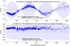 |
Fig. 6 Signature in the Doppler observable of the relativistic corrections in the rotation angle ϕ: (a) Signature (in mm s−1) of the periodic relativistic variations |
![$\left( {{{\left[ \phi \right]}_{{\rm{GR}}}}\left( t \right) - {{\dot \phi }_{{\rm{GR}}}}t} \right)$](/articles/aa/full_html/2023/02/aa44420-22/aa44420-22-eq102.png)
Geodetic precession and nutation in longitude for the planets of the Solar System (in mas, t is the time in years).
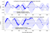 |
Fig. 7 Signature in the Doppler observable of the relativistic corrections in the longitude angle ψ: (a) Signature in the Doppler observable (in μm s−1) of the small geodetic nutations in the longitude angle as a function of time, using the RISE timing (Nov. 2018–April 2022). The blue envelope uses a simulated continuous timing. The gray dashed line represents the geodetic nutations, arbitrarily rescaled. (b) Signature in the Doppler observable (in mm s−1) of all the geodetic terms (nutations and the linear term), using the RISE timing. |
5.2 Rotation variations due to time coordinate transformation
In Table 6, we present estimates for the Sun contribution to the relativistic variations in ϕ, for a rotation model expressed in the BCRS, assuming that the planets follow Keplerian orbits (see toy model of Sect. 3.1.1). This two-body contribution tends to increase with increasing distance from the Sun, the maximum being reached for Saturn. The linear term includes for all planets the LB contribution for the rescaling between TCB and TDB (see Eq. (28)).
Table 7 provides estimates for the contribution related to the Sun motion relative to the SSB, based on the toy model of Sect. 3.1.2. For each planet, seven terms at synodic periods corresponding the indirect effects of the other planets are computed. Most of these contributions have negligible amplitude. Only the giant planets induce indirect effects on the other planets larger than 0.01 mas in amplitude, and this effect is almost zero on Mercury and Venus. The largest term (with an amplitudes above 4 mas) applies to Saturn and is caused by Jupiter.
In Table 8, we compute the contribution related to the direct effect of the planets on each other, based on the toy model of Sect. 3.1.3. For each planet, we give the total rate of the linear term due to all the other planets and the amplitudes of the seven individual terms at synodic periods. The linear terms are very small, as already noticed for Mars. As for the indirect terms, the synodic direct terms are mainly induced by the giant planets, with quasi zero effect for Mercury and Venus, and the largest term (with an amplitudes above 1 mas) applies to Saturn and is caused by Jupiter.
The results presented in this section depend on the chosen values for the parameters and in particular on the values of the eccentricities. Here, we use the eccentricities obtained from the mean orbital elements of Simon et al. (2013). If necessary, the results can be refined by a fit to a numerical integration (as in Sect. 3.2) or from a semi-analytical solution (as in Sect. 3.3).
Amplitudes of synodic terms (in mas) in the relativistic variations in ϕ, related to the Sun motion relative to the SSB, based on the toy model of Sect. 3.1.2.
6 Discussion and conclusions
We have included relativistic corrections in the orientation and rotation model of Mars expressed in the BCRS. We estimated the corrections in the Euler angles (ψ, ε, ϕ) describing the orientation of a frame attached to the surface of Mars with respect to its mean orbit. Given the current accuracy on radioscience orbiter and lander data, a precision of 0.1 mas in the relativistic corrections is required to avoid errors in the interpretation of measurements of Mars rotation in terms of local physics. An accurate estimation of the relativistic corrections in rotation is also useful to define IAU standards for the rotation and orientation of Mars (Yseboodt et al., in prep.).
We first considered the relativistic terms that impact directly the rotation, finding that only the geodetic precession induces a significant effect and this is only in longitude, ψ. Then we investigated the terms that arise in the rotation angle, ϕ, because of the time coordinate transformation between a local Mars reference fame and the BCRS. For the longitude correction, our results are in agreement with previous findings, whereas this is not the case for the rotation correction. There is no significant relativistic correction that applies to the obliquity, ε.
Therefore, our recommendations for the relativistic corrections in Mars’ Euler angles (in mas) are as follows:
![${\left[ \psi \right]_{{\rm{GR}}}}\left( t \right) = 6.754t + 0.565\sin l',$](/articles/aa/full_html/2023/02/aa44420-22/aa44420-22-eq125.png) (46a)
(46a)
![${\left[ \varepsilon \right]_{{\rm{GR}}}}\left( t \right) = 0,$](/articles/aa/full_html/2023/02/aa44420-22/aa44420-22-eq126.png) (46b)
(46b)
![$\matrix{ {{{\left[ \phi \right]}_{{\rm{GR}}}}\left( t \right)} \hfill & { = 7.3088d - 166.954\sin l' - 7.783\sin 2l'} \hfill \cr {} \hfill & { - 0.544\sin 3l' + 0.567\sin \left( {{{2\pi } \over {2.235294}}t + 320^\circ .997} \right)} \hfill \cr {} \hfill & { + 0.102\sin \left( {{{2\pi } \over {2.009124}}t + 303^\circ .752,} \right)} \hfill \cr }$](/articles/aa/full_html/2023/02/aa44420-22/aa44420-22-eq127.png) (46c)
(46c)
with t and d the time in years and days, respectively, and l′ as the mean anomaly of Mars as given in Eq. (41c). For the longitude angle, we kept the linear and annual terms of Eq. (13), estimated from a Keplerian toy model, which is consistent with the results of Baland et al. (2020). The precision on those terms is of about 0.05%, as estimated from the difference with a semi-analytical derivation based on VSOP87 ephemerides (not shown here). The linear term in [ψ]GR of 6.754 mas yr−1 is important, making a difference in the angle up to 135 mas around the year 2020. For the rotation angle, we kept the linear term and the five largest periodic terms, based on an average of the fit to the numerical solution of Table 2 and of the semi-analytical solution of Table 3. The linear term in [ϕ]GR of 7.3 mas day−1 is very large, shifting the rotation angle by 53,000 mas around the year 2020, namely, moving the prime meridian by almost 850 m in 20 yr. The accuracy of the linear term is of the order of 10−5%, the difference between the two solutions. The precision on the periodic terms is better than 0.01 mas. The last two terms are at the Mars-Jupiter (2.24yr) and Mars-Saturn (2.01 yr) synodic periods. We note that the phase of these synodic terms is not obtained as the difference between the phases of the mean anomalies of Mars and of the other planet.
Our recommendation for the expression of [ϕ]GR(t) replaces the estimate of Yoder & Standish (1997, reminded in Eq. (3)), where only the three main periodic terms are given, with an error of about 9 mas on the annual term. Such a difference can already have an effect in the radioscience data analysis, since the periods of these terms are the same as the periods of the rotation variations induced by atmosphere and surface dynamics. The synodic terms are here computed for the first time. Since their period is close the orbital period of Mars (1.88 yr), we recommend to include them in the a priori rotation model of Mars in order to avoid any contamination of the rotation amplitudes fitted to the radio-science data. Not taking them into account would likely affect the estimate of the annual term in ϕ by 0.6 mas and 0.1 mas, respectively (if the annual term absorbs their full contribution).
The applied methods (analytical, numerical, and semi-analytical) presented in this study can be extended to other bodies orbiting the Sun. In Sect. 5.2, we already demonstrated an application of the analytical toy model to other planets of the Solar System. These results can be refined by a fit to a numerical integration or from a semi-analytical solution. The methods should also be upgraded to moons, such as the Galilean moons.
Rate of the linear term and amplitudes of the synodic terms (in mas) in the relativistic variations in φ, due to the direct effects of the planets, based on the toy model of Sect. 3.1.3.
Acknowledgements
We thank the editor and an anonymous reviewer for their careful reading and comments that have helped to improve our paper. This work was financially supported by the Belgian PRODEX program managed by the European Space Agency in collaboration with the Belgian Federal Science Policy Office. This is InSight contribution ICN 304.
References
- Acton, C., Bachman, N., Semenov, B., & Wright, E. 2018, Planet. Space Sci., 150, 9 [Google Scholar]
- Acton, C. H. 1996, Planet. Space Sci., 44, 65 [Google Scholar]
- Archinal, B. A., Acton, C. H., A’Hearn, M. F., et al. 2018, Celest. Mech. Dyn. Astron., 130, 22 [Google Scholar]
- Baland, R.-M., Yseboodt, M., Le Maistre, S., et al. 2020, Celest. Mech. Dyn. Astron., 132, 47 [NASA ADS] [CrossRef] [Google Scholar]
- Barker, B. M., & O’Connell, R. F. 1970, Phys. Rev. D, 2, 1428 [NASA ADS] [CrossRef] [Google Scholar]
- Bernus, L., Minazzoli, O., Fienga, A., et al. 2019, Phys. Rev. Lett., 123, 161103 [Google Scholar]
- Bernus, L., Minazzoli, O., Fienga, A., et al. 2022, Phys. Rev. D, 105, 044057 [NASA ADS] [CrossRef] [Google Scholar]
- Bretagnon, P., & Francou, G. 1988, A&A, 202, 309 [NASA ADS] [Google Scholar]
- Brumberg, V. A., & Kopejkin, S. M. 1989, Nuovo Cimento B Serie, 103, 63 [NASA ADS] [CrossRef] [Google Scholar]
- Damour, T., Soffel, M., & Xu, C. 1991, Phys. Rev. D, 43, 3273 [Google Scholar]
- Dehant, V., Le Maistre, S., Baland, R.-M., et al. 2020, Planet. Space Sci., 180, 104776 [NASA ADS] [CrossRef] [Google Scholar]
- Eroshkin, G. I., & Pashkevich, V. V. 2007, Artif. Satellites, 42, 59 [NASA ADS] [CrossRef] [Google Scholar]
- Fienga, A., Laskar, J., Kuchynka, P., et al. 2011, Celest. Mech. Dyn. Astron., 111, 363 [Google Scholar]
- Folkner, W. M., Kahn, R. D., Preston, R. A., et al. 1997a, J. Geophys. Res., 102, 4057 [NASA ADS] [CrossRef] [Google Scholar]
- Folkner, W. M., Yoder, C. F., Yuan, D. N., Standish, E. M., & Preston, R. A. 1997b, Science, 278, 1749 [CrossRef] [Google Scholar]
- Folkner, W. M., Dehant, V., Le Maistre, S., et al. 2018, Space Sci. Rev., 214, 100 [NASA ADS] [CrossRef] [Google Scholar]
- Fukushima, T. 1991, A&A, 244, L11 [NASA ADS] [Google Scholar]
- Fukushima, T. 1995, A&A, 294, 895 [NASA ADS] [Google Scholar]
- Fukushima, T. 2010, in IAU Symposium, 261, eds. S. A. Klioner, P. K. Seidelmann, & M. H. Soffel, 89 [Google Scholar]
- Harada, W., & Fukushima, T. 2003, AJ, 126, 2557 [NASA ADS] [CrossRef] [Google Scholar]
- Irwin, A. W., & Fukushima, T. 1999, A&A, 348, 642 [NASA ADS] [Google Scholar]
- Kahan, D. S., Folkner, W. M., Buccino, D. R., et al. 2021, Planet. Space Sci., 199, 105208 [NASA ADS] [CrossRef] [Google Scholar]
- Klioner, S. A., & Voinov, A. V. 1993, Phys. Rev. D, 48, 1451 [Google Scholar]
- Konopliv, A. S., Yoder, C. F., Standish, E. M., Yuan, D.-N., & Sjogren, W. L. 2006, Icarus, 182, 23 [NASA ADS] [CrossRef] [Google Scholar]
- Konopliv, A. S., Asmar, S. W., Folkner, W. M., et al. 2011, Icarus, 211, 401 [NASA ADS] [CrossRef] [Google Scholar]
- Konopliv, A. S., Park, R. S., Rivoldini, A., et al. 2020, Geophys. Res. Lett., 47, e90568 [NASA ADS] [CrossRef] [Google Scholar]
- Kopejkin, S. M. 1988, Celest. Mech., 44, 87 [NASA ADS] [CrossRef] [Google Scholar]
- Moisson, X., & Bretagnon, P. 2001, Celest. Mech. Dyn. Astron., 80, 205 [NASA ADS] [CrossRef] [Google Scholar]
- Moyer, T. D. 1981, Celest. Mech., 23, 33 [NASA ADS] [CrossRef] [Google Scholar]
- Murray, C. D., & Dermott, S. F. 2000, Solar System Dynamics (Cambridge University Press) [Google Scholar]
- Park, R. S., Folkner, W. M., Williams, J. G., & Boggs, D. H. 2021, AJ, 161, 105 [NASA ADS] [CrossRef] [Google Scholar]
- Pashkevich, V. V. 2016, Artif. Satellites, 51, 61 [NASA ADS] [CrossRef] [Google Scholar]
- Petit, G., Luzum, B., et al. 2010, IERS Tech. Note, 36, 1 [NASA ADS] [Google Scholar]
- Pijpers, F. P. 1998, MNRAS, 297, L76 [NASA ADS] [CrossRef] [Google Scholar]
- Poisson, E., & Will, C. M. 2014, Gravity (Cambridge University Press) [Google Scholar]
- Reasenberg, R. D., & King, R. W. 1979, J. Geophys. Res., 84, 6231 [NASA ADS] [CrossRef] [Google Scholar]
- Simon, J. L., Francou, G., Fienga, A., & Manche, H. 2013, A&A, 557, A49 [NASA ADS] [CrossRef] [EDP Sciences] [Google Scholar]
- Soffel, M., Klioner, S. A., Petit, G., et al. 2003, AJ, 126, 2687 [Google Scholar]
- Standish, E. M. J. 1982, A&A, 114, 297 [NASA ADS] [Google Scholar]
- Yoder, C. F., & Standish, E. M. 1997, J. Geophys. Res., 102, 4065 [NASA ADS] [CrossRef] [Google Scholar]
- Yseboodt, M., Dehant, V., & Péters, M.-J. 2017, Planet. Space Sci., 144, 74 [NASA ADS] [CrossRef] [Google Scholar]
Except e.g. in Konopliv et al. (2011) or Reasenberg & King (1979) where the relativistic correction is written separately from the terms of Eq. (1).
All Tables
Parameter values used for computing the relativistic contributions to the Mars BCRS rotation model, in the frame of analytical and toy model developments of Sects. 2.2 and 3.1, where the orbit of the planets are assumed to be Keplerian.
Maximal amplitude of the signature in the range and the Doppler observables of the relativistic variations in the rotation angles for a lander in Elysium Planitia and using the RISE timing.
Geodetic precession and nutation in longitude for the planets of the Solar System (in mas, t is the time in years).
Amplitudes of synodic terms (in mas) in the relativistic variations in ϕ, related to the Sun motion relative to the SSB, based on the toy model of Sect. 3.1.2.
Rate of the linear term and amplitudes of the synodic terms (in mas) in the relativistic variations in φ, due to the direct effects of the planets, based on the toy model of Sect. 3.1.3.
All Figures
|
Fig. 1 Euler angles between the rotating body frame of Mars (axes XYZ) and the inertial frame associated with the mean orbit of Mars of 1980 (axes xyz, the x-axis is in the direction of the ascending node of Mars's orbit over the Earth ecliptic of epoch J2000). The X-axis of the BF is chosen as the prime meridian defined in the IAU convention (Archinal et al. 2018). The spin axis longitude ψ is measured from the x-axis to the autumn equinox, ϕ is measured from the equinox to the X-axis, and the obliquity, ε, is the angle from the z-axis to the Z-axis – or the inclination of the BF equator over the IF xy plane. |
| In the text | |
|
Fig. 2 Difference between the [ϕ]GR(t) obtained by numerically integrating Eq. (17), using the DE440 planetary ephemerides and using Eq. (25) and the fitted series from Eq. (37). This curve provides an estimate of the accuracy of the fitted analytical model provided by the coefficients from Table 2. |
| In the text | |
|
Fig. 3 Impact of the 1/c4 term from Eq. (17) on the BCRS modeling of Mars’s rotation (top). Impact of the Sun quadrupole moment |
| In the text | |
|
Fig. 4 Difference between the solutions for [ϕ]GR(t) obtained using VSOP87 and DE440 ephemerides via numerical integrations (left). Difference between the numerical integration and the semi-analytical solution using VSOP87, with only the 11 terms of Table 3 in blue, with all terms in black (right). |
| In the text | |
|
Fig. 5 Difference between the [ϕ]GR(t) of the semi-analytical solution using VSOP87 (with only the 11 terms of Table 3) and the fit of the numerical integration with DE440 ephemerides. |
| In the text | |
|
Fig. 6 Signature in the Doppler observable of the relativistic corrections in the rotation angle ϕ: (a) Signature (in mm s−1) of the periodic relativistic variations |
| In the text | |
|
Fig. 7 Signature in the Doppler observable of the relativistic corrections in the longitude angle ψ: (a) Signature in the Doppler observable (in μm s−1) of the small geodetic nutations in the longitude angle as a function of time, using the RISE timing (Nov. 2018–April 2022). The blue envelope uses a simulated continuous timing. The gray dashed line represents the geodetic nutations, arbitrarily rescaled. (b) Signature in the Doppler observable (in mm s−1) of all the geodetic terms (nutations and the linear term), using the RISE timing. |
| In the text | |
Current usage metrics show cumulative count of Article Views (full-text article views including HTML views, PDF and ePub downloads, according to the available data) and Abstracts Views on Vision4Press platform.
Data correspond to usage on the plateform after 2015. The current usage metrics is available 48-96 hours after online publication and is updated daily on week days.
Initial download of the metrics may take a while.