| Issue |
A&A
Volume 679, November 2023
|
|
|---|---|---|
| Article Number | A40 | |
| Number of page(s) | 13 | |
| Section | Stellar structure and evolution | |
| DOI | https://doi.org/10.1051/0004-6361/202346088 | |
| Published online | 01 November 2023 | |
The peculiar ejecta of the nova V1425 Aquilae
1
Instituto de Física y Astronomía, Universidad de Valparaíso, Avda. Gran Bretaña 1111, Valparaíso, Chile
e-mail: claus.tappert@uv.cl
2
European Southern Observatory, Alonso de Córdova 3107, Santiago, Chile
Received:
6
February
2023
Accepted:
5
September
2023
Many important details of the mechanisms underlying the ejection of material during a (classical) nova eruption are still not understood. Here we present optical spectroscopy and narrow-band images of the nova V1425 Aql, 23 yr after the nova eruption. We find that the ejecta consist of two significantly different components. The first resembles what is commonly seen in novae, that is, a symmetric distribution centred on the position of the underlying cataclysmic binary and presenting both allowed (hydrogen and helium) and forbidden ([O III] and [N II]) transitions. The second one, on the other hand, consists of material travelling at an approximately three times higher velocity that is not visible in the allowed transitions, presents a significantly different [N II]–[O III] ratio, and is located at approximately 2.3 arcsec to the southwest of the position of the binary. Comparing the velocities and spatial extensions of the two ejecta, we find that both originated in the same nova eruption. We explore possible extrinsic and intrinsic mechanisms for the asymmetry of the high-velocity material in the form of asymmetrically distributed interstellar material and magnetic accretion, respectively, but find the available data to be inconclusive. From the expansion parallax, we derive a distance for the nova of 3.3(3) kpc.
Key words: novae / cataclysmic variables / ISM: jets and outflows
© The Authors 2023
 Open Access article, published by EDP Sciences, under the terms of the Creative Commons Attribution License (https://creativecommons.org/licenses/by/4.0), which permits unrestricted use, distribution, and reproduction in any medium, provided the original work is properly cited.
This article is published in open access under the Subscribe to Open model. Subscribe to A&A to support open access publication.
1. Introduction
In cataclysmic binary stars (CVs), a white dwarf accretes matter from a late-type main sequence star. The material is transported either via an accretion disc and a boundary layer onto the white dwarf (in the non-magnetic dwarf novae and nova-likes) or is funnelled along the magnetic field lines directly onto its magnetic pole or poles (in CVs with a strong magnetic field, so-called polars). An intermediate configuration where the magnetic field disrupts the inner part of the accretion disc is known as an intermediate polar. For comprehensive information on CVs, see Warner (1995) and Hellier (2001).
Once the white dwarf has accumulated a certain critical amount of material, a thermonuclear runaway is triggered on its surface during which the previously accreted material (or slightly less or slightly more) is ejected into the interstellar space. This event, during which the brightness of the system increases by 8−16 magnitudes, is called a (classical) nova eruption (Bode & Evans 2012; Chomiuk et al. 2021). The underlying binary system is not destroyed and recommences the accretion process within a couple of years (e.g. Retter et al. 1998; Mason et al. 2021; Murphy-Glaysher et al. 2022), making this a recurrent event. The length of a classical nova cycle is estimated to 104 − 107 yr, depending on the mass of the white dwarf and the long-term accretion rate (Townsley & Bildsten 2004; Hillman et al. 2020a,b).
The ejected material forms an expanding nova shell that is typically not spherically symmetric, but has a prolate or bipolar shape (Gill & O’Brien 1999; Naito et al. 2022) that can also present certain asymmetries (Pavana et al. 2020) and equatorial or tropical rings (Slavin et al. 1995; Porter et al. 1998). The details of the ejection process are not yet fully understood. Some studies suggest the occurrence of several ejection events with different energetics and dynamics (e.g. Aydi et al. 2020; Steinberg & Metzger 2020; Shen & Quataert 2022), with shocks between those different layers of material being responsible for the clumpy structure of the ejecta (Li et al. 2017; Harvey et al. 2020). Other cases can be explained by a single ejection event and intrinsic clumpiness (e.g. Liimets et al. 2012; Mason et al. 2018). The long-term light curves of nova eruptions show a large diversity (Strope et al. 2010), which might reflect differences in the ejection mechanisms in different novae (e.g. Mason et al. 2020).
The nova V1425 Aql was discovered on February 2, 1995, by Nakano et al. (1995) as an object of eighth magnitude, although it is likely that the real maximum with a visual magnitude of mv = 6 − 7 mag was missed by two to three weeks (Mason et al. 1996; Kolotilov et al. 1996; Kamath et al. 1997). In time-series photometric data in the I-band taken over a range of four months in 1996, when the nova had declined by approximately 7 mag, Retter et al. (1998) detected two main periodic signals at 6.14 h and 1.44 h, as well as the beat period between them. These authors interpreted the longer period corresponding to the orbital modulation, and the shorter period as the spin period of the white dwarf, making the system an intermediate polar. However, the non-detection of any modulation in X-ray data prompted Worpel et al. (2020) to speculate that this might be a misclassification, although they also note that the source was too faint to draw any firm conclusions.
Spectroscopic observations of the ejecta in the first months after the eruption showed evidence of a clumpy structure and the presence of optically thin dust and a hot ionised gas component with a low dust-to-gas ratio ≤10−3 (Mason et al. 1996; Kamath et al. 1997). Lyke et al. (2001) estimated the ejected mass to 2.5 − 4.2 × 10⁻⁵ M⊙, which is well within the typically observed range (Tarasova 2019). Ringwald et al. (1998) reported the detection of the shell in optical passbands from narrow-band imaging with the Hubble Space Telescope (HST) approximately three years after the eruption and mention the possibility of a bipolar structure in the [O III] data, whereas Sahman et al. (2015) did not find any evidence for a shell in the Hα data taken in 2014 as part of the Isaac Newton Telescope Hα Survey (IPHAS).
We obtained photometric and spectroscopic data of V1425 Aql as part of a project to determine Hα and [O III] luminosities of old nova shells (see Tappert et al. 2020) and present our analysis of these data in the subsequent sections.
2. Observations and data reduction
2.1. Pre-imaging
Because V1425 Aql cannot be unambiguously identified on the finding chart from the Downes et al. (2005) catalogue, images were taken on July 12, 2018, in the r′ (G0326) and the Hα (G0336) passbands installed on the Gemini Multi-Object Spectrograph (GMOS; Hook et al. 2004; Gimeno et al. 2016) at the Gemini-South telescope on Cerro Pachón, Chile, in preparation for the subsequent spectroscopy. One image was taken with each filter, with exposure times of 10 s for r′ and 90 s for Hα. Bias subtraction and flat-field reduction were performed using the Gemini reduction package installed in the Image Reduction and Analysis Facility (IRAF) software (Tody 1986, 1993). A number of comparison stars were measured in each frame to correct for a small positional shift between the two images and the intensity of the Hα image was scaled to roughly correspond to the value of the r′ data. Finally, subtracting the r′ image from the Hα one unambiguously revealed the nova as the brightest Hα source in the field. In Fig. 1, we present a finding chart with the identification of the nova.
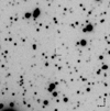 |
Fig. 1. Finding chart for V1425 Aql, based on the r′ image and centred on the position of the nova. The size is 1 × 1 arcmin and the orientation is such that east is to the left and north is up, as indicated in the lower right corner. |
We used the Graphical Astronomy and Image Analysis (GAIA1) tool in combination with the catalogue of sources identified in the Gaia mission (Gaia Collaboration 2016) to obtain an astrometric solution for the r′ image. As mentioned in Tappert et al. (2020), the nova itself is not a Gaia source. Its position was measured as the centre of the point spread function (PSF) to

which presents an offset of approximately 11 arcsec with respect to the position recorded in Downes et al. (2005), mainly due to differences in declination.
2.2. Spectroscopy
Long-slit spectroscopy was performed on September 5, 2018, using GMOS and the B600+G5323 grating. A 1.0 arcsec slit was centred on the previously determined position (Eq. (1)) with a position angle of  (measured anticlockwise from north) to avoid contamination from the object located at approximately 1.7 arcsec southeast of the nova (Fig. 1). Two series of three spectra were taken at two different central wavelengths (550 and 560 nm) to account for the gaps in the spectral coverage caused by GMOS using a mosaic of three CCDs. The individual exposure times were 400 s, resulting in a total integration time of 40 min. A 2 × 2 binning was employed, yielding a spectral resolution of 0.45 nm, measured as the full width at half maximum (FWHM) of the spectral calibration lines, and a spatial step size of 0.16 arcsec per pixel. From the acquisition image taken in the r′ filter, the FWHM of the PSF was measured as ∼0.5 arcsec.
As with the other data, the Gemini IRAF routines were applied for bias subtraction, flat-field correction, wavelength calibration, and correction for the quantum efficiency differences between the three CCDs. Subsequently, low-order functions were fitted to the sky background and subtracted. Flux calibration was obtained by comparison with the spectrophotometric standard LTT 7987 that was observed on the same night using a 5.0 arcsec slit. The resulting individual images were then averaged to yield a single spectrum (Fig. 2). The respective areas around specific emission lines were extracted so that low-order polynomials could be fitted to the stellar continuum and subsequently subtracted, which allows us to study the nova shell in detail. Examples are presented in Fig. 3. Finally, a one-dimensional spectrum at the position of the binary was established using the IRAF optimal extraction routine (Horne 1986); it is shown in Fig. 4.
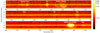 |
Fig. 2. Two-dimensional spectrum of V1425 Aql. The identified emission lines have been labelled. The spatial orientation is such that the y-axis goes from southwest to northeast at an angle of |

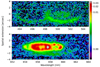 |
Fig. 3. Spectral ranges around [O III] (top) and Hα (bottom) with the stellar continuum subtracted. We refer to Fig. 2 for details of the spatial axis. |
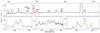 |
Fig. 4. Extracted spectrum. The upper plot presents the full available wavelength range. The data were smoothed with a filter of 7 pixels in width. Identified emission lines are labelled. The lower plots show close-ups of the unsmoothed data in the regions indicated in the upper plot by the two vertical dashed lines (Hβ, the two [O III] lines, and Hα, plus the two [N II] lines, from left to right). The vertical dashed lines indicate the nominal centres (rest wavelength plus systemic velocity) of the respective emission lines. In the rightmost plot, the letters mark the blueshifted and redshifted [N II]a,b and Hα emission line components of the inner shell, and the colour of the letters symbolises the direction of the shift. |
2.3. Narrow-band imaging
On July 25, 2019, a series of narrow-band images were taken with GMOS using Hα (G0336) and [O III] (G0338) filters as well as filters that cover the corresponding nearby continuum wavelength ranges (G0337 and G0339, hereafter HαC and [O III]C, respectively). Exposure times were kept comparatively short to avoid saturation. Further details are given in Table 1.
Parameters of the narrow-band imaging from July 25, 2019.
The Gemini IRAF routines were used for basic reduction, incorporating bias subtraction and flat-fielding. After correction of the positional shifts, all images corresponding to a specific filter were combined into a single frame using a ±1σ rejection limit. The instrumental fluxes of a number of comparison stars were measured to determine the scaling factors to be applied to the continuum data so that they match the fluxes in the emission line filters. The such scaled continuum frames were subtracted from the emission line data. The resulting emission distributions are given in Fig. 5. Measuring the FWHM of the PSF for several stars on the images, we derive a value of ∼1.1 arcsec for all filters.
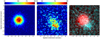 |
Fig. 5. Narrow-band images in the usual orientation with east to the left and north to the top. The left and middle plots show the Hα and the [O III] data, respectively. In both images, the sky background has been subtracted and the data have been normalised to a value of 100 with respect to their individual maximum values. The right plot shows a composite image, where the Hα data are marked in red and the [O III] data in blue. The white lines indicate the width and angle of the slit in the spectroscopic data. For all images, the zero point of the coordinate system was set to the centre of the Hα emission. |
Although the narrow-band images share an identical relative coordinate system, it proved necessary to perform an astrometric correction in order to obtain absolute positions. This was done in the same way as for the r′-band image (Sect. 2.1). The root mean squares of the coordinate fits ranged from 0.04 to 0.09 arcsec, depending on the S/N.
3. Analysis
3.1. General spectral appearance
A rough first look at the spectrum (Fig. 2) shows an unusual shell configuration, with a high-velocity component that is confined to the southwestern part of the sky. This latter is detected only in the two [O III] emission lines at λ495.9 nm and λ500.7 nm, and is somewhat weaker in [N II] λ658.4 nm. Additionally, there is a symmetric low-velocity component visible both in forbidden and allowed transitions. For the sake of brevity, we mark the blue and red lines of the forbidden transitions with “a” and “b”, respectively, as defined in Table 2. For similar reasons, throughout the paper we refer to the symmetric low-velocity ejecta as the “inner shell” and to the asymmetric high-velocity ejecta as the “outer ejecta”.
Parameters of the ejecta emission lines identified in the spectrum of V1425 Aql.
Overall, V1425 Aql presents a very rich spectrum (Fig. 4). Apart from the aforementioned forbidden lines, it includes the Balmer hydrogen series from Hα down to Hϵ, He Iλλ667.8, and 567.8 nm, He IIλλ541.2, and 468.6 nm, and the Bowen blend. The feature between He IIλ541.2 and He Iλ567.8 is most likely N IIλ568.0 nm. At its red side, there is potentially a very weak remnant of the once strong [N II] λ575.5 nm emission (Kamath et al. 1997; Lyke et al. 2001), but its intensity is too close to the noise level to identify it with any certainty. A comparison of Figs. 2 and 4 shows that most, if not all, emission lines are present in the ejecta. The only doubtful case is that of the Bowen blend, which, despite being almost as bright overall as the neighbouring He II line, shows a significantly smaller spatial extension, if any. At the very least, this line is clearly dominated by emission from the binary, either from the accretion disc or as a recombination from the illuminated side of the secondary star. For the other emission lines, the contribution from sources inside the binary appears to be mostly negligible. In the He I lines, the blueshifted and redshifted components are sufficiently separated that it should be possible to distinguish any emission from the binary, but no such feature can be detected with any confidence. In the bluer lines, such as Hβ and He II, this is more difficult, but it is clear that the emission from the ejecta is dominant. Many post-novae appear to have high mass-transfer rates (e.g. Fuentes-Morales et al. 2021), implying the presence of a bright, optically thick accretion disc, where most emission lines are weak, and V1425 Aql appears to fall into that category. In such systems, the strongest disc emission line is usually found to be Hα. Unfortunately, the strong blend of the Hα + [N II] emission from the ejecta (Fig. 4, right) prevents detection of such a component. Finally, we note that the spectrum does not present any obvious absorption lines.
3.2. Velocities and spatial extensions
The first attempt to determine velocities by fitting the emission line profiles with Gaussian functions proved unsuccessful because of several overlaps and blends both in the spatial and the spectral direction, especially in the Hα/[N II] complex (Fig. 4, right). For example, within our spectral resolution, the blueshifted component of [N II]b overlaps exactly with the redshifted one of Hα. Overall, the blending is such that there is no transition for which both the blueshifted and the redshifted components could be clearly distinguished. In addition, at least for Hα, a contribution from the accretion disc or other locations in the underlying binary can be expected. The bluer emission lines are mostly not as affected by blending as the region around Hα, but they present significantly lower S/Ns (Fig. 4, left). In most lines, this results in too many degeneracies to fit both emission line components, which would be necessary to calculate first the systemic and then the expansion velocities.
We therefore determined the wavelengths of the emission lines by drawing ellipses to represent the two-dimensional emission distribution of a given line and registering the points that coincide with the stellar continuum. The corresponding 3σ uncertainties are estimated to be in the order of ±1 pixel, which is equal to ±0.1 nm. The systemic velocity vs was determined as the centre of the two Doppler-shifted velocity components and with respect to the rest wavelength of that line. Finally, the radial velocity was calculated as the difference between the maximum observed velocity and vs. The values for the measured lines are collected in Table 2. For the outer [N II]b ejecta, the blue Doppler shift could not be determined with any sufficient precision. Therefore, in this case, we calculated the radial velocity of the red component with respect to the mean systemic velocity. The latter is obtained as the average of the individual values, excluding the outlier from the [O III]a line, to vs = 75(25) km s−1. In addition, we derive the average radial velocities for the shell of the allowed transitions, vr, a = 527(44) km s−1, for the inner shell of the forbidden lines, vr, f, i = 470(19) km s−1, and for the outer ejecta, vr, f, o = 1555(92) km s−1. This yields the ratios
which overlap within one sigma.
We tested the validity of our method by fitting the profiles of the He Iλ587.6 nm emission line components with a Gaussian, because these are the most isolated and least distorted lines. We obtained a systemic velocity of 59 km s−1, and find the velocities of the lines to be 513 km s−1, which lies well within the uncertainty range of the values determined by the comparison with ellipses above.
Next, we measured the extensions rp of the ejecta in the spatial direction. We calculated the sum of the central three to five CCD columns of a given shell line. The centres of the brightness distributions of the shell and of the stellar continuum were measured by fitting Gaussian functions to them and the extension of the shell was calculated with respect to the latter value. With the precision we achieve here, we find the inner shell to be symmetrical around the stellar continuum, and so the extensions into both directions were averaged to yield the values in Table 2. From the typical FWHM of the Gaussians, we estimate a 1σ uncertainty of two-thirds of a pixel. We find average spatial extensions of rp, a = 0.82(02) arcsec for the shell of the allowed transitions, rp, f, i = 0.69(03) arcsec for the inner shell of the forbidden lines, and rp, f, o = 2.33(08) arcsec for the outer ejecta. The ratios are then
which overlap within two sigma. From this comparison, there is therefore a possibility that the inner shell of the forbidden lines and the inner shell of the allowed lines occupy slightly different velocity and spatial regimes. Given that the two transitions need different density conditions, this is not entirely unexpected.
Comparing Eqs. (2) and (3), the velocity ratios agree very well with their respective extension ratios. Dividing the velocity by the radius ratios, we find a value of 1.04(11) for the comparison of the outer forbidden lines with the allowed lines and 0.97(09) for the comparison of the outer and inner forbidden lines. For a nova age of 23.6 yr, we can still assume a constant expansion velocity without deceleration (e.g. Santamaría et al. 2020) and therefore the above ratios are also valid for the time that has passed since the ejection of the material. As both values agree well with unity within their errors, we can conclude that both the outer ejecta and the inner shell(s) originate in the same nova eruption, with the respective uncertainties translating to time ranges of 2.6 and 2.1 yr for the outer forbidden to allowed and for the outer to the inner forbidden line regions, respectively.
3.3. Brightness distribution
The narrow-band photometry corroborates our findings from spectroscopy. While the Hα emission is placed symmetrically at the position of the nova, the [O III] distribution shows an elongated shape, with its maximum positioned to the southwest of Hα. The FWHM of the PSF of the inner shell measures 2.1 arcsec, which when compared to the value of the stellar PSF (1.1 arcsec, Sect. 2.3) shows that the emission distribution is resolved.
We determined the position of the brightness distribution by measuring the geometrical centre of the Hα image first in a contour plot and afterwards by applying the centring routine implemented in the GAIA viewer. The position of the [O III] emission is more ambiguously defined because of its asymmetric shape and the considerable noise in the data, which affects even the region of the maximum intensity (S/N ∼ 3). We opted for the centre of an ellipse with a major axis of 1.58 and a minor axis of 0.55 arcsec, which encompasses the southern “head” of the distribution (around x, y = 1, −1.5 in the coordinate system of Fig. 5), where the highest intensities are located.
This yields the coordinates

for Hα and

for [O III]. The two centres are therefore separated by 1.91(10) arcsec, which is comparable to the values measured in the spectroscopy (Table 2; we point out that the head is not fully included in the slit; see Fig. 5, right), and form an angle of 215(7)° east of north.
3.4. Expansion parallax
Assuming equal velocities in the line of sight and perpendicular to the observer, the distance d to the nova can be determined from the radial velocity vr, the projected expansion of the shell in arcsec r, and the time Δt that has passed since the nova eruption, as

With vr and r for the different ejecta as given in Sect. 3.2 and Δt = 23.6 yr for our spectroscopic data (taking January 21, 1995, as an estimated date for the nova eruption), we obtain an average of d = 3.2(3) kpc from the allowed lines, 3.4(3) kpc from the forbidden lines of the inner shell, and 3.3(3) kpc from the outer ejecta, yielding a final value of d = 3.3(3) kpc.
Previous distance estimations were provided by Mason et al. (1996) and Kamath et al. (1997) as d = 3.6 − 4.8 kpc and d = 2.7(6) kpc, respectively. Both employed the maximum magnitude rate of decline relation, whose usefulness is nevertheless still hotly debated (Schaefer 2018; Selvelli & Gilmozzi 2019; Della Valle & Izzo 2020). The difference in those two distance estimations is mainly due to the different extinctions used by the authors, with Mason et al. (1996) correcting for EB − V = 0.55 mag and Kamath et al. (1997) using EB − V = 0.76 mag. The Stilism website2 (Lallement et al. 2019) gives  mag for a limiting distance of 2.4 kpc in the direction of the nova, which favours the higher extinction value and therefore the lower distance.
The potential flaw in our distance estimate lies in the assumption that the measured radial velocity corresponds to the measured spatial extension, while in reality the two quantities concern two different parts of the ejected material. As mentioned in Sect. 1, nova shells are typically not spherically symmetric and a proper distance determination would require a model for the spatial extension in the line of sight. We also did not take any possible deceleration of the material into account. However, we note that the velocity of the outer ejecta lies well within the range of velocities observed shortly after the eruption (Mason et al. 1996; Kamath et al. 1997; Arkhipova et al. 2002), and so this is unlikely to be a significant effect.
3.5. Flux
For each shell of a given emission line in the continuum-subtracted spectroscopic data, we defined two ellipses representing the outer and inner limits of the brightness distribution (Fig. 6). We then used the EllipticalAperture routine in the Photutils package (Bradley et al. 2019) within Astropy (Astropy Collaboration 2013, 2018) to measure the respective total fluxes, calculating the shell flux as the difference. In this way, any potentially present emission from the binary is also subtracted from the data. Because the previous subtraction of the sky leaves the background centred on a zero value, this also works for the “incomplete” ellipses of the outer ejecta.
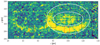 |
Fig. 6. Areas used for the flux calculation on the example of the [O III] lines in the continuum–subtracted spectrum. The ellipses represent the region used for the elliptical aperture photometry of the outer [O III]b line. The two red rectangles mark the areas of comparison between the outer [O III]a,b lines. The black rectangles indicate the region of overlap of the [O III]a line with the outer [O III]b material and the corresponding region for [O III]b. For details see the text. |
Several lines in the spectrum are affected by blending with neighbouring lines, and therefore the above method is not applicable, at the very least not without further corrections. For the inner ejecta, this concerns the Hα + [N II] region. Fortunately, it contains two line components that can be assumed to be mainly free of other contributors: the blueshifted peak of [N II]a and the redshifted peak of [N II]b (Fig. 4, right). Measuring the fluxes of the redshifted and blueshifted peak in the Hβ emission line, which represents the strongest unblended emission, we find that they differ by approximately 5%. The profile of the line shows that both peaks are likely composed of several components. In the red peak, these appear to be closer together in velocity space – yielding an overall higher intensity – than in the blue peak, where the components are more easily separated (lower left plot in Fig. 4). The other lines of the inner shell appear to show a corresponding behaviour, including the forbidden lines as indicated by the albeit more noise-affected [O III] λ501 emission (lower middle plot in Fig. 4). This can be interpreted as evidence of a certain clumpiness of the inner ejecta. We proceed by assuming that this structure and the equality of the fluxes in both peaks within 5% are valid for all inner emission lines. We now average the central three rows (roughly corresponding to the stellar PSF) of the continuum-subtracted 2D spectrum and fit Gaussian functions to the four identified peaks, corresponding to the blueshifted component of [N II]a, the combination of the blueshifted peak of Hα and the redshifted peak of [N II]a, the blend of the redshifted peak of Hα with the blueshifted peak of [N II]b, and finally the redshifted peak of [N II]b, all of which refer to the inner shell. We subtract the [N II]a,b contribution to the Hα line, which is measured on the respective undisturbed components. The results for both Hα peaks agree well with each other and we find an average flux for one Hα peak of 0.209(10)×10−18 W m−2. The ratios to the fluxes of the [N II] lines are Hα/[N II]a = 6.95 and Hα/[N II]b = 2.40.
We repeat the procedure for the inner shell of [O III]b, measuring only the better-defined red peak. This yields flux ratios [N II]b/[O III]b = 11.11 and [N II]a/[O III]b = 3.84. Because the flux for [O III]b can be measured using the elliptical aperture photometry, we can now use these factors to calculate the total fluxes contained in the slit for the two [N II] lines from the [O III]b flux. The flux of the Hα line then follows from the Hα/[N II] ratios.
The discernible emission lines of the outer ejecta, [O III]a, [O III]b, and [N II]b, also present different degrees of overlap. The most severely affected line is that of [N II]b, the blueshifted half of which is hidden within the Hα and [N II] emission from the inner shell. Thus, we calculate the fluxes by comparing the intensities of the three lines of the outer ejecta using the elliptical aperture photometry of the outer [O III]b line as the base flux, which we first have to correct for the overlap with the [O III]a line on its blue side. We assume that all three emissions track the same material and that the intensity ratios are constant over the entire spatial extension. Then, for all three lines, we can define rectangular regions that correspond to the same respective velocity and spatial range, and where all three lines are undisturbed from other contributors (for the [O III] lines; these are the red rectangles in Fig. 6). Similar to the elliptical aperture photometry, the size of those areas is not important as long as they contain the same emission portions for all three lines and exclude other emission sources, because the background is centred around zero. Comparison of the total intensities contained in these areas yields the ratios [O III]b/[O III]a = 2.86(10) and [O III]b/[N II]b = 1.47(01). The uncertainties were estimated by displacing the areas by 1 pixel in each direction and repeating the measurement.
To obtain the total flux in the slit for the [O III]b line, we can use its elliptical aperture photometry, but we have to correct for the overlap with [O III]a. We define two rectangular areas (black rectangles in Fig. 6), the first one including the complete overlap region, that is the red part of [O III]a and the blue part of [O III]b. The second area defines the red part of [O III]b, which corresponds to the same velocity and spatial range. From the intensities contained in these areas and using the above intensity ratios, we can now calculate the contribution from [O III]a to the blue part of [O III]b and correct the flux from the elliptical aperture photometry by subtracting it. The total slit fluxes of [O III]a and [N II]b are then calculated from that value divided by their respective ratios.
We estimate the total emitted flux by first rotating the narrow-band images with respect to the position angle of the spectroscopy and sum the instrumental flux of the area that corresponds to a 1.0 arcsec slit. A comparison with the total instrumental flux shows that in the case of Hα the slit contains a fraction of 0.45 of the total flux, and in the case of [O III] it contains a fraction of 0.35. In the second step, we sum the rows of the spectroscopic data that contain emission from the shell, use the SpectRes Python package (Carnall 2017) to rebin the spectra and the normalised filter curves of the four narrow-band filters (see Sect. 2.3) to a common step size, and finally multiply the spectrum with each filter curve to calculate the included flux. This yields fluxes of FHα = 8.45, FHαC = 2.85, F[OIII] = 0.89, and F[OIII]C = 0.76 × 10⁻¹⁸ W m−2 for the four filters, and therefore the differences FHα − FHαC = 5.60 and F[OIII] − F[OIII]C = 0.13 × 10⁻¹⁸ W m−2, which can now can be compared to the instrumental fluxes of the narrow-band imaging. Assuming that the above factors of 0.45 and 0.35 determined for Hα and for [O III] can be used in general for the inner and the outer ejecta, respectively, we calculate the total fluxes Ft for each emission line and shell.
As the final step, we use the Astropy dust_extinction package3 to correct the fluxes for the interstellar extinction according to Fitzpatrick (2004). We apply EB − V = 0.76 mag, because this appears to be the best estimate at present (see Sect. 3.4). The resulting fluxes are shown in Table 2.
Comparing the fluxes of the forbidden lines, we note that the two ejecta present almost opposite [N II]/[O III] ratios, because Ft, [NII]b/Ft, [OIII]b = 0.31(01) for the outer material, but 5.08(28) for the inner shell.
3.6. HST data
Hubble Space Telescope data for V1425 Aql were collected using the Wide Field Planetary Camera instrument (WFPC2) on November 19, 1997, almost three years after the nova event. A total of four images were taken in filters F469, F502, F656, and F658. Ringwald et al. (1998) present a brief summary of the data, suggesting that the F502 image, which includes the [O III] line, could show a bipolar structure with a 0.2 arcsec separation.
We reanalysed these archival data to determine whether it is possible to observe the asymmetric ejecta already at such an early stage. The target was located in the field of view of the planetary camera of the instrument, which has a pixel scale of 0.0455 arcsec pixel−1. The image had been calibrated to have physical units of W m−2 nm−1 using the standard procedure for WFPC2 images. We used the width and pivot wavelength of the filter4 to obtain physical units of W m−2 arcsec−2 and to determine AB magnitudes. Aperture photometry with a radius of 0.5 arcsec and annuli of 0.5 and 1.5 arcsec for the inner and outer radii for background subtraction yields an AB magnitude of 12.61(1) mag for V1425 Aql in the F502 filter. The FWHM of the stellar PSF is measured as ∼0.15 arcsec, while that of the nova amounts to ∼0.21. Thus, similar to the GMOS data, the nova shell is just, but clearly, resolved.
At the time of the GMOS NB observations (Δt = 24.5 yr), the asymmetric ejecta are located at a distance of 1.91(10) arcsec from the centre of the Hα emission (Sect. 3.3). Assuming a constant expansion rate, we obtain a value of 0.078(4) arcsec yr−1. Thus, at the time of HST observations, the asymmetric ejecta should be at 0.22(01) arcsec from the position of the nova.
Figure 7 shows the F502 image with the overimposed contour levels of the F656 filter. Originally, the two different emission distributions presented a small but noticeable offset of 0.025 arcsec between their centres. Measuring the positions of one of the stars in the two images, we find a very similar offset. We can therefore attribute this shift between filters to an instrumental effect and have corrected this correspondingly for the plot. There, the position where we expect to observe the asymmetric ejecta is marked with a cross.
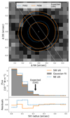 |
Fig. 7. Flux distribution of the HST data. The top plot shows the contours of the F656 and the F502 flux overlaid on the F656 image, representing fractions of 0.5, 0.1, and 0.05 of the respective central fluxes. The F502 data have been corrected for the small instrumental shift (see text). The white cross marks the expected position of the outer [O III] ejecta, with the sizes of the marker denoting the uncertainty in the radial distance and angle. The lines mark the area used to derive the radial profile shown in the middle plot. Dashed and solid lines represent the flux in the two directions towards and away from the expected outer ejecta, while the filled area indicates a Gaussian fit. The bottom plot presents the respective residuals to that fit. |
We note that the two emission distributions occupy the same area, and that they can be well described by a circle, especially at lower intensities. The only exception is in the centre of the F502 emission, which presents a certain elongation. However, this latter lies roughly perpendicular to the direction in which the outer ejecta would be expected and is therefore unlikely to be connected with it.
We test for a possible excess in flux at the expected position of the ejecta by comparing the radial profile of the F502 distribution in the direction of the ejecta and in the opposite direction. For this purpose, we define a “slit” area in which we sum up the pixel values as a function of the distance from the centre of the distribution (middle and bottom plot in Fig. 7). We conclude that no excess emission is observed near that position.
To investigate the evolution of the inner shell, we compare the HST F656 data with the GMOS Hα image. For this, we first have to find common ground for the respective astrometries, and must therefore refer to the r′-band image (Fig. 1), because GMOS Hα and F656 do not have any common stars. We find one star in the F656 image that is (barely) not saturated in r′ and can be used for comparison. This star is also in the Gaia Data Release 3 catalogue, which lists its coordinates as  and proper motions as −0.871(20) and −2.422(18) mas yr−1 in right ascension and declination, respectively. Correcting for the proper motion that corresponds to the time difference between F656 and r′ observations, we find offsets of ΔαF656 − r′ = 0.51 arcsec and ΔδF656 − r′ = 0.08 arcsec. The difference between the GMOS r′-band and Hα images is negligible, because both astrometries were corrected with respect to the Gaia catalogue. Taking the above shift into account, we now find that the centre of the GMOS Hα emission differs from that in the F656 observation by ΔαF656 − Hα = 0.12 arcsec and ΔδF656 − Hα = 0.29 arcsec, amounting to 0.31 arcsec in total, and in the direction of 201° east of north.
Finally, we employ aperture photometry to determine the fluxes F in the two filters. Using a large aperture of 0.65 arcsec (compare to Fig. 7) yields F(Hα) = 1.53 × 10⁻¹⁶ W m−2 and F([OIII]) = 1.17 × 10⁻¹⁶ W m−2, and, when corrected for interstellar extinction, F(Hα) = 7.92 × 10⁻¹⁶ W m−2 and F([OIII]) = 1.33 × 10⁻¹⁵ W m−2. In the following section, we show how these fluxes relate to previously determined values and the GMOS data.
3.7. Flux evolution
The evolution of the luminosity of nova shells was originally investigated by Downes et al. (2001) and later refined by Tappert et al. (2020) who limited the sample to systems with a well-known distance and grouped the data according to speed class and to the light-curve classification scheme introduced by Strope et al. (2010). The authors defined three different phases in the long-term evolution of the nova shell flux for both the Hα and the [O III] emission: a roughly constant behaviour in the initial and late stages, and a linear decline slope in between (on a double logarithmic scale). These three stages were interpreted as corresponding to the transition from optically thick to optically thin material, the free expansion phase, and the start of the interaction with the interstellar medium (ISM), respectively. The slopes and time intervals that define the three sections appear to vary somewhat with respect to light curve type and/or speed class, but most data sets suffered from incomplete sampling, leaving room for significant systematic uncertainties.
Because V1425 Aql has not been detected by Gaia, it was not part of the Tappert et al. (2020) study, although Downes et al. (2001) incorporated the flux data from Kamath et al. (1997) in their catalogue. With the above fluxes derived from the HST and GMOS observations, the data on V1425 Aql now cover a much larger time range. For a comparison of the decline slopes, we do not need the conversion to luminosity, because this only results in a different vertical zero point. Therefore, we can avoid the uncertainty related to distance and interstellar extinction. Because the flux values in Table 2 are already extinction corrected, we collect all the “raw” flux data used in this section in Table 3. As we show in Sect. 4.2, we can assume that emission from the outer ejecta was below the detection limit in the HST data. For consistency, we limit the analysis of the flux evolution to the inner shell.
Flux data.
The data are plotted in Fig. 8. According to Strope et al. (2010), V1425 Aql is a member of the S-class, which presents smooth decline light curves. For this class, Tappert et al. (2020) find that for Hα, the initial, roughly constant, stage corresponds to a time interval of log(Δt) = [−2.0, −1.0], the decline stage to [ − 1.3, 1.4], and the late, again roughly constant, stage corresponds to [0.9, 1.8]. For [O III], the corresponding values are [ − 1.2, −0.4], [ − 0.5, 1.2], and [0.9, 1.7], respectively. The fact that some of these ranges overlap is evidence for the aforementioned incomplete sampling. Unfortunately, the available data on V1425 Aql suffer from the same problem, presenting two large gaps from approximately 0.4 to 2 yr and from 3 to 20 yr. Taking the above ranges for the S-class, for [O III], the data before the first gap should correspond to the initial “constant” phase, the data in between the gaps to the decline, and the final data point (the GMOS flux) to the late “constant” phase. For Hα, all data before the second gap should be part of the decline, whereas the last data point possibly corresponds to the late stage. However, as mentioned above, those Δt limits are not very well defined. We therefore decided to fit two functions to each data set. The first is fit to three data points: the last one before the first gap and the two before the second gap. This yields slopes of −2.86(22) for Hα and of −2.32(12) for [O III]. The second function is a fit to the latter two data points with the slope fixed to the value for the S-class, namely −2.52(06) and −3.78(28), respectively.
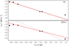 |
Fig. 8. Hα (top) and [O III] (bottom) flux vs. time on a double logarithmic scale. The dashed lines represent fits to the three data points within −0.6 < log(Δt) < 0.6, while the dotted lines were fitted to the two points near log(Δt) = 0.4 with fixed respective slopes of the S-class from Tappert et al. (2020). |
The patchy sampling of both the Tappert et al. (2020) and the V1425 Aql data certainly necessitates a large amount of caution in interpreting the results. Still, we find that they at least fit into a consistent picture. For Hα, the two slopes overlap within 1.5σ, and also the first two data points not included in the fit agree well with the resulting slope. However, the GMOS flux lies clearly above that decline. All data points before the second gap can therefore be regarded as being part of the decline phase, while the GMOS observations already show the late phase in the Hα evolution. On the other hand, the slopes for the [O III] data differ by almost 5σ. It is therefore likely that all data before the first gap still belong to the constant phase and so the inclusion of the last one of those points in the fit yields a slope that is too shallow. Assuming a steeper slope, as for Hα, the GMOS [O III] flux could also already correspond to the late phase, although the offset from the decline slope is not as pronounced. Fitting only the three data points after the first gap yields a slope of −2.95(16), which overlaps with the S-class slope within 3σ.
4. Discussion
4.1. One or two shells?
At first glance, the V1425 Aql data suggest the presence of two distinctive ejecta that cover different velocity and spatial regimes. We find that they originate in the same nova eruption, but our precision leaves a time range of approximately ±2 yr between the actual ejection events. During recent years, evidence has accumulated that – at least in some novae – the ejection of material in the eruption is not a single event, but takes place in stages and involves different ejection velocities (Friedjung 2011; Chomiuk et al. 2021). The typical picture is that of an early slow ejection in the equatorial plane and a subsequent high-velocity bipolar outflow that can occur up to several hundred days later (Woudt et al. 2009; Chomiuk et al. 2014). We emphasise that our time resolution, based on the velocities and distances, allows for both a single ejection scenario and for two ejections with a time difference of up to approximately two years. We also note that the long-term light curve of the nova provided by the American Association of Variable Star Observers (AAVSO)5 within this time range presents a scatter (at times up to slightly more than 1 mag) and a coverage (including two gaps with a length of ≥two months) that would allow a minor or even a significant rebrightening – that could have accompanied a second ejection – to remain undetected. Furthermore, the light curve in Strope et al. (2010), although classified as “smooth” between Δt ∼ 60 and 90 d, presents a clear bump with a size of approximately 0.5 mag. Such bumps and other fluctuations occur in many novae, including some systems of the S-class, and are not conclusive evidence for additional ejections. However, their largely unknown origin leaves room for a number of possibilities (e.g. Mason et al. 2020, who explain jitters and oscillations in nova light curves by unstable nuclear burning on the WD).
The two emission regions clearly present different densities, with that of the outer one being too low to enable allowed transitions. In principle, this distribution could also represent a single asymmetric shell. Indeed, we note that the offset of 0.31 arcsec of the centre of the Hα emission with respect to the HST data is at an angle similar to the location of the outer [O III] material (Sect. 3.6), which could reflect a general tendency of the ejecta to move in that direction. However, the FWHM of the GMOS Hα shell amounts to approximately 2.2 arcsec and, considering that the astrometric comparison between HST and GMOS is based on a single star, it is not certain that the observed offset is really significant. Photometry under good seeing conditions and in a spectral range that avoids the main emission from the shell could allow us to pinpoint the location of the underlying binary and thus clarify whether or not the inner shell is symmetrically placed around the post-nova.
A finding in favour of the interpretation of two ejecta is the fact that both the [O III] and [N II] emission distributions present a local intensity minimum between the inner and outer emission regions, both in space and in velocity. This indicates that the emission distribution cannot be explained by a gradually decreasing density. The spatial separation is not discernible in the [O III] narrow-band image, which does not show any clear presence of the inner shell. However, this is likely due to the large flux difference between the two ejecta for this transition (Table 2). In fact, the 2D spectrum (Fig. 2), where the inner [O III] shell is clearly detected, does not reflect the real flux difference, because the slit covers a larger fraction of the inner shell than that of the outer ejecta. As can be seen in Fig. 5, even the maximum of the [O III] distribution is significantly affected by noise. Therefore, the apparent absence of the inner shell in that image can be explained by low S/N and the significantly poorer seeing conditions in the narrow-band images compared with those associated with the spectroscopic data (1.1 arcsec vs. 0.5 arcsec; Sects. 2.2 and 2.3, respectively).
4.2. Intrinsic or extrinsic?
Deviations from axial symmetry in nova shells are well known. For example, the shell of IPHASX J210204.7+471015 presents a severe asymmetry, including a strong spatial separation of the Hα and the [O III]-emitting material (Santamaría et al. 2019), and Schaefer et al. (2019) list a number of other examples. However, these concern mainly comparatively old novae (IPHASX J210204.7+471015 has a suspected age of 130 to 170 yr), where the observed asymmetries are likely caused by interaction of the ejecta with inhomogeneously distributed ISM. On the other hand, it has been speculated that intrinsic non-axisymmetric ejections could be common and that they could play an important role in the evolution of CVs, causing temporary orbital eccentricities with consequences for the mass-transfer process (Nelemans et al. 2016; Schaefer et al. 2019).
Therefore, in principle, there are two possibilities: either the observed asymmetry of the outer ejecta is due to interaction with asymmetrically distributed ISM, or it is due to an intrinsic effect, meaning an asymmetric ejection mechanism. To investigate the former possibility, we examined data from the Wide-field Infrared Survey Explorer (WISE; Wright et al. 2010), which is available in four wavelength bands centred on 3.4, 4.6, 12.1, and 22 μm, respectively. Of special interest for our case are the latter two, with band 3 being sensitive to hot ISM and band 4 sensitive to cold dust.
The band 3 data indeed present an asymmetric distribution of ISM close to the position of the nova, with an intensity gradient that rises from north to south (left plot of Fig. 9). However, because we do not know the distance of that feature, it is unclear as to whether it is really in the vicinity of the nova or whether this is just a projection effect. Still, let us assume for a moment that this ISM band indeed causes the originally (axis-)symmetrically ejected material to be seen as a comparatively isolated blob. As the gradient increases towards the outer ejecta, the asymmetry would therefore have to be caused not by obscuration of one part of the ejecta, but by excitation; that is, in the northeastern part, the ISM is not sufficiently dense to interact with the ejecta, and thus the latter remains invisible, while in the southwestern direction, the ejecta plough into the more concentrated ISM, with part of the shock energy being transformed into radiation. However, this interpretation has several problems. First, while the gradient is increasing towards the south, there is still material present north of the nova, and so it is hard to imagine that there would be no interaction at all in that region. Second, even if the extension of the inner shell is only approximately one-third of that of the outer ejecta, some effect of asymmetric ISM should still be visible, which is not the case. Finally, this possibility requires the radiation from the outer ejecta to be exclusively caused by interaction with the ISM. From the flux evolution (Sect. 3.7), we find indeed that such interaction is likely to contribute to the flux for the inner shell, and thus even more probably to the outer ejecta. However, the distance of the asymmetric blob to the binary amounts to approximately 1 × 10¹² km = 0.032 pc, using vexp = 1550 km s−1 and Δt = 23.6 yr. At that distance, the material should still be affected by photoionisation (compare e.g. with the shell of V382 Vel, which has a radius of ≈0.045 pc; Takeda & Diaz 2019) and it is not clear why this should affect only one side of a hypothetically symmetric ejecta.
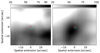 |
Fig. 9. WISE data of the 40 × 40 arcsec field centred on V1425 Aql. The left and right plots show the band 3 and band 4 images, respectively. As in the other maps, the orientation is north up, east to the left. Both linear colour maps have an intensity range of 20% (white) to 100% (black) of the intensity range in the shown area. The circles mark the positions of the two ejecta. The size of the circles also roughly corresponds to the extension of the ejecta. |
The WISE band 4 data, which are sensitive to colder material, do not show any enhancement in the northeastern direction that could obscure emission from ejecta in that region either. Instead, there is a concentration at a distance of approximately 3.4 arcsec southeast of the nova; it is unlikely to be related to the nova, because if it were a remnant of a previous nova eruption at a – again hypothetical – former position of V1425 Aql, one would expect a roughly ring-like distribution, which is very different from the observed one. In any case, the location of the centre of the distribution makes it unlikely that it causes the asymmetry in the outer ejecta.
Looking for an intrinsic origin for the asymmetry, we need to identify a mechanism that provides an isolated and well-defined location on the surface of the white dwarf. The one process that immediately springs to mind is accretion along the magnetic field lines that deposits the material from the donor star onto one of the magnetic poles. As mentioned in Sect. 1, some observations identify V1425 Aql as an intermediate polar (Retter et al. 1998), whereas others suggest that the magnetic field is rather weak (Worpel et al. 2020). In the latter case, it is unlikely that it would have any effect on the nova eruption (Livio et al. 1988).
Finally, the HST data (Sect. 3.6) have the potential to distinguish between an extrinsic and an intrinsic origin, because they were taken at a significantly earlier time after the eruption than the GMOS data, but still at a point where the separation of the two ejecta would have already been discernible. However, the fact that the inner shell is detected but the outer ejecta are not means the case remains inconclusive. Considering that the GMOS data show the outer material to be significantly brighter in [O III] than the inner shell (Table 2), the ratio of the [O III] flux of the two ejecta must have been reversed at some point between the two data sets. In principle, a possible reason for this could be that the F502 filter data of the inner shell contain a strong contribution from the continuum of the binary, which would not be present in the outer ejecta. However, the spectra presented by Kamath et al. (1997) and Lyke et al. (2001), both taken roughly 2.3 yr after the eruption – which is approximately half a year before the HST data–, indicate that the filter will almost exclusively have sampled the emission of the two [O III] lines. Therefore, for the flux ratio to become inverted, the [O III] flux of the inner shell must have suffered a steeper initial decline than that of the outer ejecta and/or the latter must have experienced an increase at a later stage. As the GMOS flux lies below the detection limit of the HST observations, we cannot decide which scenario applies. From our analysis of the flux evolution (Sect. 3.7), the GMOS [O III] emission of the inner shell could possibly already include a contribution from interaction with the ISM. Because the outer shell has covered a significantly larger distance, one could speculate that it experiences a stronger effect of this kind.
Also, the assumption of a constant expansion rate of the outer ejecta could be wrong. Instead, it could have been ejected a considerable amount of time later than the inner shell, as has been observed for the (symmetric) high-velocity material in V445 Pup (Woudt et al. 2009) and V959 Mon (Chomiuk et al. 2014), meaning that at the time of the HST observations, it was still too close to the inner shell to be resolved. This implies that its velocity was initially larger than the current value and consequently experienced a braking due to interaction with the ISM. Still, this would require the presence of sufficiently dense ISM in that region, for which we find no indication from the WISE data. We also note that velocity-wise deviations from free expansion are typically expected to occur for novae that are much older than V1425 Aql (Duerbeck 1987; Santamaría et al. 2020).
4.3. Temperature, density, or abundances?
From Sect. 3.5, we note that the [O III]–[N II] ratio is very different for the two ejecta, with [O III] being much more prominent in the outer material. The transitions of both lines are strongly dependent on temperature and density (Osterbrock & Ferland 2006), and so these are the parameters that are most likely to be responsible for the difference. On the other hand, in principle, the two ejection processes could also have involved different mixing, meaning that more material from the inner parts of the white dwarf was dredged up for one ejection than for the other, resulting in different abundances in the ejecta.
In their analysis of data taken approximately 820 d after the eruption, Lyke et al. (2001) find two classes of material with two different densities and velocities, which they interpret as evidence for the “clumpiness of the ejecta”. Their measured line FWHMs are spread between 550 and 1600 km s−1 and are clearly influenced by mixing from the various line-emitting regions. As none of the shell components had yet been resolved, light at different velocities and from different shell components is mixed in the PSF. Nevertheless, the highest ionised lines associated with a density ne of 3.5 × 104 cm−3 and a temperature of 13 800 K show an average FWHM of approximately 1500 ± 100 km s−1, while the neutral lines, which are associated with densities of 2.1 − 4.6 × 105 cm−3 for temperatures of 10 000–15 000 K on average show velocities of approximately 1080 ± 55 km s−1. These velocities are fairly consistent with our measurements, taking half the FWHM as the velocity of a radially symmetric expanding shell and the full FWHM as the velocity of a plume or shell that is only ejected in one direction. In hindsight, we might therefore interpret the denser “clumps” described by Lyke et al. (2001) as the beginning what we now see as the dense, inner shell, while the low-density material they measured turned into the outer shell ejected only to one side.
We can test how the densities of these two components have evolved and extrapolate them assuming that no further material was added to the shell. This assumption is reasonable as the measurements of Lyke et al. (2001) are from day 820, while the white dwarf nuclear burning turnoff already occurred on day 400. We also assume that the radius of the shell at turnoff defines the thickness of the sphere D = 400 d × vej, which then continues to freely expand in the radial direction with a constant velocity vej. We use vi = 500 km s−1 (i.e. roughly half the FWHM) for the slow, high-density shell component and vo = 1500 km s−1 for the fast, low-density component. For a constant amount of material, we can use ne(8624 d) = ne(820 d)×V(820 d)/V(8624 d) for the volumes V at the respective times and derive the electron densities at the time of the GMOS observations for the two shell components as ni = 1.37 − 3.01 × 103 cm−3 and no = 0.23 × 103 cm−3. Both values are sufficiently low to be considered at the low-density limit, which allows us to derive the temperature from the respective [O III] and [N II] line ratios (Osterbrock & Ferland 2006).
Unfortunately, with [O III] λ436.3 nm and [N II] λ575.5 nm, both ratios involve lines that are not detected in our data. We derive upper flux limits from the 3σ variation of the background in our spectrum. For [O III], we find Fi(λ436.3) < 4 × 10⁻²⁰ W m−2 and Fo(λ436.3) < 5 × 10⁻²⁰ W m−2, which yields upper limits for the temperatures of Ti, [OIII] < 12 000 K and To, [OIII] < 7500 K for the inner and outer shell, respectively. For [N II], we derive Fi(λ575.5) < 4 × 10⁻²⁰ W m−2 and Fo(λ575.5) < 3 × 10⁻²⁰ W m−2, yielding Ti, [NII] < 5000 K and To, [NII] < 7800 K. Although these upper limits are not conclusive for exploring the differences between the two ejecta, they are reasonable in that they are below the value derived by Lyke et al. (2001) and above the temperatures expected for older nova shells (e.g. Osterbrock & Ferland 2006).
Both extrapolated densities are too low to have any significant effect on the forbidden emissions, and so these depend mainly on their transition probabilities. Therefore, the difference in the densities in the two ejecta cannot explain the observed difference in the line ratios between [O III] and [N II]. In fact, because the latter transition is the “most forbidden” one (Wiese et al. 1996), a higher density should have a quenching effect on [N II] rather than on [O III]. However, in our data, [N II] is stronger than [O III] in the denser, inner shell and weaker in the outer ejecta. Therefore, we only see two possible causes of this difference: abundance or temperature. Our data are not suitable for measuring the abundances of either of the two shell components. We can only say that if the two components were ejected at different moments of the nova eruption, a different mix between dredged-up and accreted material could have been ejected, and so this explanation remains a possibility. Concerning the temperature, it is likely – although unproven because we only have upper limits – that the inner shell has a lower temperature than the outer ejecta. Because the D2 level of [O III] needs a higher energy to be populated than the corresponding level in [N II], we could be in a position where the different temperatures of the shell components simply provide the perfect conditions in the sense that the D2 level of [O III] is still populated normally in the outer shell but not in the inner one; therefore, the [O III] lines are quenched and become weaker. We would like to stress that while this is a possible scenario, it cannot be supported with our data.
5. Summary and conclusions
We present spectroscopic and narrow-band imaging data of the nova V1425 Aql that show the emission distribution of the ejecta approximately 23 yr after maximum brightness. We find that the material ejected during the nova eruption consists of two distinctively different components: one low-velocity component and one high-velocity component (referred to throughout the paper as the inner shell and outer ejecta, respectively). The former is likely situated symmetrically around the nova and is detected in the hydrogen, He I, and He II emission lines, as well as in the [O III] and [N II] transitions. There is some indication that the material seen in the forbidden lines and the material seen in the allowed ones occupy slightly different velocities and spatial regimes, but this is not conclusive, because the values still agree within two sigma. From the profiles of the emission lines, we find evidence of inhomogeneities in the ejected material, confirming the findings of Kamath et al. (1997) and Lyke et al. (2001).
The outer material has an elongated shape with maximum brightness situated 1.91(10) arcsec at an angle of 215(7)° east of north from the nova. The ratios of velocity and spatial extensions for the low- and high-velocity ejecta are such that we can conclude that they originated in the same event, although not necessarily at the same time. The two ejecta have significantly different [N II]–[O III] line ratios, likely due to different temperatures and/or abundances.
With the available data, we are unable to distinguish between an external and an intrinsic origin of the asymmetry of the high-velocity material. Intuitively, the latter appears more likely, but the evidence is inconclusive. Comparison of the Hα and [O III] flux evolution since the nova eruption with other novae suggests that some of the emission is caused by interaction with the ISM. However, we did not find any evidence for an inhomogeneous distribution of the latter that could explain the observed asymmetry.
The main purpose of this paper is to draw attention to the existence of this – to our knowledge – unprecedented phenomenon. We did not attempt to model the geometry of the nova ejecta (e.g. Gill & O’Brien 1999; Ribeiro et al. 2013), because recently acquired integral field unit spectroscopy with the Multi Unit Spectroscopic Explorer (MUSE) will directly provide the 3D distribution of the material. A detailed analysis of these data will be published elsewhere (Celedón et al., in prep.).
Last but not least, we point out that the discovery of these unusual ejecta was achieved because a close field star was located at such an angle that it forced us to place the slit in a certain direction that coincided with the distribution of the ejecta. As deep spectroscopic surveys or deep narrow-band imaging studies involving an [O III] filter of medium-aged nova shells are rare, it appears possible that similar phenomena could be present in other novae as well, which would have significant implications for our understanding of the ejection mechanism.
Acknowledgments
We thank the referee, Elena Mason, for her thorough review and stimulating discussion, which led to many improvements and broadening of the scope of the paper. The ejecta of V1425 Aql and nova eruptions in general were topics of many pleasant discussions with Steve Shore at the University of Pisa during a brief but very fruitful stay of one of the authors (CT). Many thanks for a wonderful and insightful time. We would also like to thank Timo Kravtsov for his valuable suggestions in interpreting the emission line ratios. C.T. acknowledges financial support from Conicyt-Fondecyt grant No. 1170566. L.C. acknowledges economic support from ANID-Subdireccion de capital humano/doctorado nacional/2022-21220607. Based on observations obtained at the international Gemini Observatory, a program of NSF’s NOIRLab, which is managed by the Association of Universities for Research in Astronomy (AURA) under a cooperative agreement with the National Science Foundation on behalf of the Gemini Observatory partnership: the National Science Foundation (United States), National Research Council (Canada), Agencia Nacional de Investigación y Desarrollo (Chile), Ministerio de Ciencia, Tecnología e Innovación (Argentina), Ministério da Ciência, Tecnologia, Inovações e Comunicações (Brazil), and Korea Astronomy and Space Science Institute (Republic of Korea). Observing IDs: GS-2018B-Q-132, GS-2018B-Q-230, GS-2019B-Q-130. The data were processed using the Gemini IRAF package. Based on observations made with the NASA/ESA Hubble Space Telescope, and obtained from the Hubble Legacy Archive, which is a collaboration between the Space Telescope Science Institute (STScI/NASA), the Space Telescope European Coordinating Facility (ST-ECF/ESA) and the Canadian Astronomy Data Centre (CADC/NRC/CSA) This research has made use of the NASA/IPAC Infrared Science Archive, which is funded by the National Aeronautics and Space Administration and operated by the California Institute of Technology.
References
- Arkhipova, V. P., Burlak, M. A., & Esipov, V. F. 2002, Astron. Lett., 28, 100 [NASA ADS] [CrossRef] [Google Scholar]
- Astropy Collaboration (Robitaille, T. P., et al.) 2013, A&A, 558, A33 [NASA ADS] [CrossRef] [EDP Sciences] [Google Scholar]
- Astropy Collaboration (Price-Whelan, A. M., et al.) 2018, AJ, 156, 123 [Google Scholar]
- Aydi, E., Chomiuk, L., Izzo, L., et al. 2020, ApJ, 905, 62 [NASA ADS] [CrossRef] [Google Scholar]
- Bode, M. F., & Evans, A. 2012, Classical Novae (Cambridge, UK: Cambridge University Press) [Google Scholar]
- Bradley, L., Sipőcz, B., Robitaille, T., et al. 2019, https://doi.org/10.5281/zenodo.3568287 [Google Scholar]
- Carnall, A. C. 2017, ArXiv e-prints [arXiv:1705.05165] [Google Scholar]
- Chomiuk, L., Linford, J. D., Yang, J., et al. 2014, Nature, 514, 339 [NASA ADS] [CrossRef] [Google Scholar]
- Chomiuk, L., Metzger, B. D., & Shen, K. J. 2021, ARA&A, 59, 391 [NASA ADS] [CrossRef] [Google Scholar]
- Della Valle, M., & Izzo, L. 2020, A&ARv, 28, 3 [NASA ADS] [CrossRef] [Google Scholar]
- Downes, R. A., Duerbeck, H. W., & Delahodde, C. E. 2001, J. Astron. Data, 7, 6 [Google Scholar]
- Downes, R. A., Webbink, R. F., Shara, M. M., et al. 2005, J. Astron. Data, 11, 2 [Google Scholar]
- Duerbeck, H. W. 1987, Ap&SS, 131, 461 [NASA ADS] [CrossRef] [Google Scholar]
- Fitzpatrick, E. L. 2004, ASP Conf. Ser., 309, 33 [NASA ADS] [Google Scholar]
- Friedjung, M. 2011, A&A, 536, A97 [NASA ADS] [CrossRef] [EDP Sciences] [Google Scholar]
- Fuentes-Morales, I., Tappert, C., Zorotovic, M., et al. 2021, MNRAS, 501, 6083 [Google Scholar]
- Gaia Collaboration (Prusti, T., et al.) 2016, A&A, 595, A1 [NASA ADS] [CrossRef] [EDP Sciences] [Google Scholar]
- Gill, C. D., & O’Brien, T. J. 1999, MNRAS, 307, 677 [NASA ADS] [CrossRef] [Google Scholar]
- Gimeno, G., Roth, K., Chiboucas, K., et al. 2016, SPIE Conf. Ser., 9908, 99082S [NASA ADS] [Google Scholar]
- Harvey, E. J., Redman, M. P., Boumis, P., et al. 2020, MNRAS, 499, 2959 [CrossRef] [Google Scholar]
- Hellier, C. 2001, Cataclysmic Variable Stars (New York: Springer) [Google Scholar]
- Hillman, Y., Shara, M. M., Prialnik, D., & Kovetz, A. 2020a, Nat. Astron., 4, 886 [Google Scholar]
- Hillman, Y., Shara, M., Prialnik, D., & Kovetz, A. 2020b, Adv. Space Res., 66, 1072 [CrossRef] [Google Scholar]
- Hook, I. M., Jørgensen, I., Allington-Smith, J. R., et al. 2004, PASP, 116, 425 [NASA ADS] [CrossRef] [Google Scholar]
- Horne, K. 1986, PASP, 98, 609 [Google Scholar]
- Kamath, U. S., Anupama, G. C., Ashok, N. M., & Chandrasekhar, T. 1997, AJ, 114, 2671 [NASA ADS] [CrossRef] [Google Scholar]
- Kolotilov, E. A., Tatarnikov, A. M., Shenavrin, V. I., & Yudin, B. F. 1996, Astron. Lett., 22, 729 [Google Scholar]
- Lallement, R., Babusiaux, C., Vergely, J. L., et al. 2019, A&A, 625, A135 [NASA ADS] [CrossRef] [EDP Sciences] [Google Scholar]
- Li, K.-L., Metzger, B. D., Chomiuk, L., et al. 2017, Nat. Astron., 1, 697 [Google Scholar]
- Liimets, T., Corradi, R. L. M., Santander-García, M., et al. 2012, ApJ, 761, 34 [NASA ADS] [CrossRef] [Google Scholar]
- Livio, M., Shankar, A., & Truran, J. W. 1988, ApJ, 330, 264 [NASA ADS] [CrossRef] [Google Scholar]
- Lyke, J. E., Gehrz, R. D., Woodward, C. E., et al. 2001, AJ, 122, 3305 [NASA ADS] [CrossRef] [Google Scholar]
- Mason, C. G., Gehrz, R. D., Woodward, C. E., et al. 1996, ApJ, 470, 577 [NASA ADS] [CrossRef] [Google Scholar]
- Mason, E., Shore, S. N., De Gennaro Aquino, I., et al. 2018, ApJ, 853, 27 [Google Scholar]
- Mason, E., Shore, S. N., Kuin, P., & Bohlsen, T. 2020, A&A, 635, A115 [NASA ADS] [CrossRef] [EDP Sciences] [Google Scholar]
- Mason, E., Shore, S. N., Drake, J., et al. 2021, A&A, 649, A28 [NASA ADS] [CrossRef] [EDP Sciences] [Google Scholar]
- Murphy-Glaysher, F. J., Darnley, M. J., Harvey, É. J., et al. 2022, MNRAS, 514, 6183 [NASA ADS] [CrossRef] [Google Scholar]
- Naito, H., Tajitsu, A., Ribeiro, V. A. R. M., et al. 2022, ApJ, 932, 39 [NASA ADS] [CrossRef] [Google Scholar]
- Nakano, S., Takamizawa, K., Kushida, Y., et al. 1995, IAU Circ., 6133, 1 [Google Scholar]
- Nelemans, G., Siess, L., Repetto, S., Toonen, S., & Phinney, E. S. 2016, ApJ, 817, 69 [NASA ADS] [CrossRef] [Google Scholar]
- Osterbrock, D. E., & Ferland, G. J. 2006, Astrophysics of Gaseous Nebulae and Active Galactic Nuclei (Sausalito, CA: University Science Books) [Google Scholar]
- Pavana, M., Raj, A., Bohlsen, T., et al. 2020, MNRAS, 495, 2075 [NASA ADS] [CrossRef] [Google Scholar]
- Porter, J. M., O’Brien, T. J., & Bode, M. F. 1998, MNRAS, 296, 943 [NASA ADS] [CrossRef] [Google Scholar]
- Retter, A., Leibowitz, E. M., & Kovo-Kariti, O. 1998, MNRAS, 293, 145 [Google Scholar]
- Ribeiro, V. A. R. M., Bode, M. F., Darnley, M. J., et al. 2013, MNRAS, 433, 1991 [NASA ADS] [CrossRef] [Google Scholar]
- Ringwald, F. A., Wade, R. A., Orosz, J. A., & Ciardullo, R. B. 1998, Am. Astron. Soc. Meet. Abstr., 192, 53.04 [NASA ADS] [Google Scholar]
- Sahman, D. I., Dhillon, V. S., Knigge, C., & Marsh, T. R. 2015, MNRAS, 451, 2863 [NASA ADS] [CrossRef] [Google Scholar]
- Santamaría, E., Guerrero, M. A., Ramos-Larios, G., et al. 2019, MNRAS, 483, 3773 [Google Scholar]
- Santamaría, E., Guerrero, M. A., Ramos-Larios, G., et al. 2020, ApJ, 892, 60 [CrossRef] [Google Scholar]
- Schaefer, B. E. 2018, MNRAS, 481, 3033 [NASA ADS] [CrossRef] [Google Scholar]
- Schaefer, B. E., Boyd, D., Clayton, G. C., et al. 2019, MNRAS, 487, 1120 [NASA ADS] [CrossRef] [Google Scholar]
- Selvelli, P., & Gilmozzi, R. 2019, A&A, 622, A186 [NASA ADS] [CrossRef] [EDP Sciences] [Google Scholar]
- Shen, K. J., & Quataert, E. 2022, ApJ, 938, 31 [NASA ADS] [CrossRef] [Google Scholar]
- Slavin, A. J., O’Brien, T. J., & Dunlop, J. S. 1995, MNRAS, 276, 353 [CrossRef] [Google Scholar]
- Steinberg, E., & Metzger, B. D. 2020, MNRAS, 491, 4232 [NASA ADS] [CrossRef] [Google Scholar]
- Strope, R. J., Schaefer, B. E., & Henden, A. A. 2010, AJ, 140, 34 [NASA ADS] [CrossRef] [Google Scholar]
- Takeda, L., & Diaz, M. 2019, PASP, 131, 054205 [NASA ADS] [CrossRef] [Google Scholar]
- Tappert, C., Vogt, N., Ederoclite, A., et al. 2020, A&A, 641, A122 [NASA ADS] [CrossRef] [EDP Sciences] [Google Scholar]
- Tarasova, T. N. 2019, Astrophysics, 62, 475 [NASA ADS] [CrossRef] [Google Scholar]
- Tody, D. 1986, SPIE Conf. Ser., 627, 733 [Google Scholar]
- Tody, D. 1993, ASP Conf. Ser., 52, 173 [NASA ADS] [Google Scholar]
- Townsley, D. M., & Bildsten, L. 2004, ApJ, 600, 390 [NASA ADS] [CrossRef] [Google Scholar]
- Warner, B. 1995, Cataclysmic Variable Stars (Cambridge, NY: Cambridge University Press) [CrossRef] [Google Scholar]
- Wiese, W. L., Fuhr, J. R., & Deters, T. M. 1996, Atomic Transition Probabilities of Carbon, Nitrogen, and Oxygen: A Critical Data Compilation (Melville, NY: AIP Press) [Google Scholar]
- Worpel, H., Schwope, A. D., Traulsen, I., Mukai, K., & Ok, S. 2020, A&A, 639, A17 [NASA ADS] [CrossRef] [EDP Sciences] [Google Scholar]
- Woudt, P. A., Steeghs, D., Karovska, M., et al. 2009, ApJ, 706, 738 [Google Scholar]
- Wright, E. L., Eisenhardt, P. R. M., Mainzer, A. K., et al. 2010, AJ, 140, 1868 [Google Scholar]
All Tables
Parameters of the ejecta emission lines identified in the spectrum of V1425 Aql.
All Figures
|
Fig. 1. Finding chart for V1425 Aql, based on the r′ image and centred on the position of the nova. The size is 1 × 1 arcmin and the orientation is such that east is to the left and north is up, as indicated in the lower right corner. |
| In the text | |
|
Fig. 2. Two-dimensional spectrum of V1425 Aql. The identified emission lines have been labelled. The spatial orientation is such that the y-axis goes from southwest to northeast at an angle of |
| In the text | |
|
Fig. 3. Spectral ranges around [O III] (top) and Hα (bottom) with the stellar continuum subtracted. We refer to Fig. 2 for details of the spatial axis. |
| In the text | |
|
Fig. 4. Extracted spectrum. The upper plot presents the full available wavelength range. The data were smoothed with a filter of 7 pixels in width. Identified emission lines are labelled. The lower plots show close-ups of the unsmoothed data in the regions indicated in the upper plot by the two vertical dashed lines (Hβ, the two [O III] lines, and Hα, plus the two [N II] lines, from left to right). The vertical dashed lines indicate the nominal centres (rest wavelength plus systemic velocity) of the respective emission lines. In the rightmost plot, the letters mark the blueshifted and redshifted [N II]a,b and Hα emission line components of the inner shell, and the colour of the letters symbolises the direction of the shift. |
| In the text | |
|
Fig. 5. Narrow-band images in the usual orientation with east to the left and north to the top. The left and middle plots show the Hα and the [O III] data, respectively. In both images, the sky background has been subtracted and the data have been normalised to a value of 100 with respect to their individual maximum values. The right plot shows a composite image, where the Hα data are marked in red and the [O III] data in blue. The white lines indicate the width and angle of the slit in the spectroscopic data. For all images, the zero point of the coordinate system was set to the centre of the Hα emission. |
| In the text | |
|
Fig. 6. Areas used for the flux calculation on the example of the [O III] lines in the continuum–subtracted spectrum. The ellipses represent the region used for the elliptical aperture photometry of the outer [O III]b line. The two red rectangles mark the areas of comparison between the outer [O III]a,b lines. The black rectangles indicate the region of overlap of the [O III]a line with the outer [O III]b material and the corresponding region for [O III]b. For details see the text. |
| In the text | |
|
Fig. 7. Flux distribution of the HST data. The top plot shows the contours of the F656 and the F502 flux overlaid on the F656 image, representing fractions of 0.5, 0.1, and 0.05 of the respective central fluxes. The F502 data have been corrected for the small instrumental shift (see text). The white cross marks the expected position of the outer [O III] ejecta, with the sizes of the marker denoting the uncertainty in the radial distance and angle. The lines mark the area used to derive the radial profile shown in the middle plot. Dashed and solid lines represent the flux in the two directions towards and away from the expected outer ejecta, while the filled area indicates a Gaussian fit. The bottom plot presents the respective residuals to that fit. |
| In the text | |
|
Fig. 8. Hα (top) and [O III] (bottom) flux vs. time on a double logarithmic scale. The dashed lines represent fits to the three data points within −0.6 < log(Δt) < 0.6, while the dotted lines were fitted to the two points near log(Δt) = 0.4 with fixed respective slopes of the S-class from Tappert et al. (2020). |
| In the text | |
|
Fig. 9. WISE data of the 40 × 40 arcsec field centred on V1425 Aql. The left and right plots show the band 3 and band 4 images, respectively. As in the other maps, the orientation is north up, east to the left. Both linear colour maps have an intensity range of 20% (white) to 100% (black) of the intensity range in the shown area. The circles mark the positions of the two ejecta. The size of the circles also roughly corresponds to the extension of the ejecta. |
| In the text | |
Current usage metrics show cumulative count of Article Views (full-text article views including HTML views, PDF and ePub downloads, according to the available data) and Abstracts Views on Vision4Press platform.
Data correspond to usage on the plateform after 2015. The current usage metrics is available 48-96 hours after online publication and is updated daily on week days.
Initial download of the metrics may take a while.