| Issue |
A&A
Volume 678, October 2023
|
|
|---|---|---|
| Article Number | A129 | |
| Number of page(s) | 16 | |
| Section | Extragalactic astronomy | |
| DOI | https://doi.org/10.1051/0004-6361/202347175 | |
| Published online | 13 October 2023 | |
Calibrating mid-infrared emission as a tracer of obscured star formation on H II-region scales in the era of JWST
1
INAF – Osservatorio Astrofisico di Arcetri, Largo E. Fermi 5, 50125 Florence, Italy
e-mail: This email address is being protected from spambots. You need JavaScript enabled to view it.
2
Department of Astronomy, The Ohio State University, 140 West 18th Avenue, Columbus OH 43210, USA
3
Sub-department of Astrophysics, Department of Physics, University of Oxford, Keble Road, Oxford OX1 3RH, UK
4
European Southern Observatory, Karl-Schwarzschild Straße 2, 85748 Garching bei München, Germany
5
Argelander-Institut für Astronomie, Universität Bonn, Auf dem Hügel 71, 53121 Bonn, Germany
6
Instituto de Alta Investigación, Universidad de Tarapacá, Casilla 7D, Arica, Chile
7
Max-Planck-Institut für Extraterrestrische Physik (MPE), Giessenbachstrasse 1, 85748 Garching, Germany
8
Sterrenkundig Observatorium, Ghent University, Krijgslaan 281-S9, 9000 Gent, Belgium
9
European Southern Observatory (ESO), Alonso de Córdova 3107, Casilla 19, Santiago 19001, Chile
10
Department of Physics and Astronomy, University of Wyoming, Laramie, WY 82071, USA
11
Astronomisches Rechen-Institut, Zentrum für Astronomie der Universität Heidelberg, Mönchhofstraße 12-14, 69120 Heidelberg, Germany
12
Univ. Lyon, Univ. Lyon1, ENS de Lyon, CNRS, Centre de Recherche Astrophysique de Lyon UMR5574, 69230 Saint-Genis-Laval, France
13
Universität Heidelberg, Zentrum für Astronomie, Institut für theoretische Astrophysik, Albert-Ueberle-Straße 2, 69120 Heidelberg, Germany
14
International Centre for Radio Astronomy Research, University of Western Australia, 7 Fairway, Crawley, 6009 WA, Australia
15
Universität Heidelberg, Interdisziplinäres Zentrum für Wissenschaftliches Rechnen, Im Neuenheimer Feld 205, 69120 Heidelberg, Germany
16
Max-Planck-Institute for Astronomy, Königstuhl 17, 69117 Heidelberg, Germany
17
Observatorio Astronómico Nacional (IGN), C/Alfonso XII, 3, 28014 Madrid, Spain
18
Department of Physics, University of Alberta, Edmonton, AB T6G 2E1, Canada
19
Departamento de Física de la Tierra y Astrofísica, Universidad Complutense de Madrid, 28040 Madrid, Spain
20
Instituto de Física de Partículas y del Cosmos IPARCOS, Facultad de CC Físicas, UCM, 28040 Madrid, Spain
21
Department of Astronomy & Astrophysics, University of California, San Diego, 9500 Gilman Drive, San Diego, CA 92093, USA
22
Department of Physics and Astronomy, McMaster University, 1280 Main St. West, Hamilton, ON L8S 4M1, Canada
23
Canadian Institute for Theoretical Astrophysics (CITA), University of Toronto, 60 St George Street, Toronto, ON M5S 3H8, Canada
Received:
13
June
2023
Accepted:
1
September
2023
Abstract
Measurements of the star formation activity on cloud scales are fundamental to uncovering the physics of the molecular cloud, star formation, and stellar feedback cycle in galaxies. Infrared (IR) emission from small dust grains and polycyclic aromatic hydrocarbons (PAHs) is widely used to trace the obscured component of star formation. However, the relation between these emission features and dust attenuation is complicated by the combined effects of dust heating from old stellar populations and an uncertain dust geometry with respect to heating sources. We used images obtained with NIRCam and MIRI as part of the PHANGS–JWST survey to calibrate the IR emission at 21 μm, and the emission in the PAH-tracing bands at 3.3, 7.7, 10, and 11.3 μm as tracers of obscured star formation. We analysed ∼20 000 optically selected H II regions across 19 nearby star-forming galaxies, and benchmarked their IR emission against dust attenuation measured from the Balmer decrement. We modelled the extinction-corrected Hα flux as the sum of the observed Hα emission and a term proportional to the IR emission, with aIR as the proportionality coefficient. A constant aIR leads to an extinction-corrected Hα estimate that agrees with those obtained with the Balmer decrement with a scatter of ∼0.1 dex for all bands considered. Among these bands, 21 μm emission is demonstrated to be the best tracer of dust attenuation. The PAH-tracing bands underestimate the correction for bright H II regions, since in these environments the ratio of PAH-tracing bands to 21 μm decreases, signalling destruction of the PAH molecules. For fainter H II regions, all bands suffer from an increasing contamination from the diffuse IR background. We present calibrations that take this effect into account by adding an explicit dependence on 2 μm emission or stellar mass surface density.
Key words: dust / extinction / galaxies: ISM / galaxies: star formation / infrared: ISM
© The Authors 2023
 Open Access article, published by EDP Sciences, under the terms of the Creative Commons Attribution License (https://creativecommons.org/licenses/by/4.0), which permits unrestricted use, distribution, and reproduction in any medium, provided the original work is properly cited.
This article is published in open access under the Subscribe to Open model. This email address is being protected from spambots. You need JavaScript enabled to view it. to support open access publication.
1. Introduction
Interstellar dust biases our view of star formation, obscuring the ultraviolet (UV) and optical emission of newly formed massive stars. The energy absorbed by dust at short wavelengths is re-radiated in the infrared (IR), making observations of dust emission a powerful probe of embedded star formation. Multi-wavelength studies, at both low and high redshift, have highlighted the importance of the IR to provide a full account of star formation rates (SFRs) in galaxies (Calzetti et al. 2007; Wuyts et al. 2011a; Kennicutt & Evans 2012; Gruppioni et al. 2013; Madau & Dickinson 2014; Calzetti 2020).
The thermal dust emission spectrum peaks in the far-IR. In the limit where the dust heating is dominated by young stellar populations, the far-IR emission can be directly related to the embedded SFR using energy balance (Kennicutt 1998). However, such a bolometric measure of dust luminosity is sensitive to heating by older stellar populations (Cortese et al. 2008). This heating term contributes progressively more to the cooler, longer wavelength far-IR emission, leading to diffuse ‘IR cirrus’. On the other hand, the mid-IR (MIR) region around 24 μm, corresponding to the IRAS 25 μm, the Spitzer MIPS 24 μm band, or the WISE W4 (22 μm) filter, traces emission of small, hot grains. While not directly relatable to the bolometric dust luminosity without further assumptions on the shape of the dust spectral energy distribution (SED), emission at 24 μm has the advantage of tracing a hotter dust component, and therefore being less sensitive to IR cirrus.
Several authors have advocated for the use of 24 μm fluxes, in combination with either UV or Hα recombination line emission, to account for both the attenuated and un-attenuated component of the SFR (Hirashita et al. 2003; Kennicutt et al. 2007, 2009; Calzetti et al. 2007; Wuyts et al. 2011b; Hao et al. 2011; Leroy et al. 2012; Kennicutt & Evans 2012; Jarrett et al. 2013; Catalán-Torrecilla et al. 2015; Leslie et al. 2018). These hybrid recipes have been demonstrated to be successful for both integrated galaxies and kiloparsec-scale sub-galactic regions in local galaxies (Calzetti et al. 2007; Leroy et al. 2012; Belfiore et al. 2023). However, dust heating from old stellar populations can still constitute a significant fraction of a galaxy’s integrated emission at 24 μm (Bendo et al. 2012; Groves et al. 2012; Crocker et al. 2013; Lu et al. 2015; Boquien et al. 2016; Viaene et al. 2017) and complicates the association of the MIR with star formation in observations that have low spatial resolution (Leroy et al. 2012).
In addition to 24 μm, several authors have studied the potential of using the flux in polycyclic aromatic hydrocarbons (PAH) features or the brightness of PAH-tracing bands (most commonly the IRAC 8 μm band) to probe obscured star formation (Peeters et al. 2004; Shipley et al. 2016; Maragkoudakis et al. 2018; Whitcomb et al. 2020). These calibrations offer significant advantages with respect to the longer mid-IR wavelengths in terms of angular resolution and sensitivity (Calzetti 2020; Li 2020). Moreover, PAH features remain accessible and are readily identifiable with Spitzer, and now the James Webb Space Telescope (JWST), out to high redshifts (Lutz et al. 2005; Riechers et al. 2014). Studies of nearby galaxies at high spatial resolution have demonstrated, however, that PAH emission is suppressed relative to 24 μm (or total IR) emission at the position of H II regions (Helou et al. 2004; Bendo et al. 2006; Bolatto et al. 2007; Lebouteiller et al. 2011; Chastenet et al. 2019, 2023a; Egorov et al. 2023). In particular, PAH emission is found to generate bright rings around H II regions, probably due to PAH photo-destruction, therefore complicating the relation between PAHs and star formation (Galliano et al. 2018).
In this work, we test the use of both the MIR dust continuum at 21 μm and bands dominated by PAH emission to trace embedded star formation on the scale of individual H II regions (∼40 − 110 pc) in a sample of 19 nearby disc galaxies observed with the MIRI and NIRCam instruments onboard JWST as part of the PHANGS (Physics at High Angular resolution in Nearby Galaxies) JWST url (Lee et al. 2023). We compare the attenuation estimates obtained using literature calibrations based on the MIR/Hα ratios with matched-resolution Balmer decrement (Hα/Hβ) measurements obtained from the PHANGS–MUSE integral field spectroscopy (IFS) mapping with the VLT/MUSE instrument (Emsellem et al. 2022).
Using this JWST data, we calibrate photometric measurements of the MIR continuum and PAH emission to accurately trace the obscured component of star formation on scales of individual H II regions. Our analysis builds on the work of Leroy et al. (2023b) and Hassani et al. (2023), who used early data for a subset of four galaxies in our sample to demonstrate that attenuation-corrected Hα emission correlates well with MIR emission at 21 μm, albeit non-linearly, for regions that are bright in the MIR.
In Sect. 2 we present our data, paying special attention to the new JWST images, and summarise the methods for inferring the dust attention. In Sect. 3 we present our results concerning the use of the IR bands in correcting Hα for dust attenuation in H II regions, and discuss the recommended recipes and potential future work in Sect. 4. We summarise the results in Sect. 5.
2. Data and methods
2.1. PHANGS–JWST data
We analysed 19 galaxies observed as part of the cycle 1 PHANGS–JWST Treasury programme (ID 02107, PI: J. Lee). The survey consists of MIRI and NIRCam images for galaxies observed by the PHANGS–MUSE programme (Emsellem et al. 2022). Key properties of our target galaxies are summarised in Table 1.
Key properties of the PHANGS–MUSE sample of galaxies used in this work.
For each target we obtained one or more NIRCam and MIRI tiles, covering roughly the same area on sky and maximising the overlap with existing MUSE observations. MIRI images were obtained in the F770W, F1000W, F1130W and F2100W filters, centred at 7.7, 10, 11.3, and 21 μm, respectively. With NIRCam we obtained images in the F200W, F300M, F335M, and F360M filters, centred at 2.0, 3.0, 3.37, and 3.6 μm, respectively. NIRCam and MIRI observations were obtained in sequence, in order to obtain a MIRI background pointing in parallel with the NIRCam observations. However, for three galaxies (IC 5332, NGC 4303, NGC 4321) all or part of the NIRCam observations were not obtained due to guide star failures. In the case of IC 5332 NIRCam data was obtained during a subsequent visit, while for NGC 4303 and NGC 4321 only one NIRCam tile was obtained out of the intended two-tile mosaic, therefore covering roughly half of the area imaged with MIRI. Because of the failure of the first NIRCam visit for IC 5332, to process its MIRI data the background frame for NGC 7496 (taken on the same day) was used.
The observing strategy and data reduction workflow are presented in Lee et al. (2023) and Williams et al. (in prep.), respectively. Here we briefly discuss specific reduction steps of particular importance for this work, and which represent an update with respect to the early reduction process described in Lee et al. (2023). We used the latest version of the CRDS context (jwst_1070) and science calibration pipeline (v1.10.0). Secondly, we have implemented a custom background matching technique to minimise the per-pixel difference in each pair of overlapping tiles. The JWST pipeline assumes a constant background across the image, which is not the case for our observations (in many cases, one half of the image has a significantly lower ‘background’ level than the other). Our routine avoids this by calculating the median per-pixel difference in each overlapping pair, and finding values that minimise this across the tile set. Thirdly, we have improved the absolute astrometry for the long wavelength MIRI tiles, by basing the astrometric solution of the longer bands on that of the shortest MIRI band (F770W). As each tile in each filter is observed close in time, and using the same guide stars, this produces significantly better astrometric solutions than attempting to match each band separately. Finally, as discussed in Leroy et al. (2023b) the background level of the overall image mosaics are re-scaled to match those of existing Spitzer or WISE data. This step is necessary because we generally do not have empty sky regions that can used for background subtraction within our mosaics.
We convolved the JWST images to match the MUSE point spread function (PSF), which is different for each target as discussed in the next subsection. The required kernels were generated using the methodology of Aniano et al. (2011) and the JWST PSFs were obtained via the WebbPSF tool (Perrin et al. 2014). Error maps produced by the JWST reduction pipeline were also convolved with the same kernels and the errors are propagated analytically through the convolution process. For one galaxy, NGC 4535, the MUSE PSF full width at half maximum (FWHM) (0.56″) is smaller than the F2100W PSF. We therefore convolve the JWST data with the smallest suitable kernel (an ‘aggressive’ kernel in the definition of Aniano et al. 2011) to generate an image with a Gassian PSF. The resulting PSF FWHM is of 0.71″ FWHM, and the MUSE maps for this galaxy are smoothed to the same PSF.
In the NIRCam wavelength range, the PAH emission feature at 3.3 μm falls in the F335M medium-band filter. As discussed in Sandstrom et al. (2023a), we performed a bespoke continuum subtraction procedure using the adjoining F300M and F360M medium-band filters in order to remove stellar continuum emission and minimise the impact of the PAH emission contaminating the F360M side-band. Our procedure is based on and improves upon the scheme first suggested by Lai et al. (2020). In this work we refer to the resulting continuum-subtracted emission as
 (1)
(1)
where F335Mcont is the continuum contamination estimated using Eqs. (10) and (11) from Sandstrom et al. (2023a). For the rest of this work we only work with the continuum-subtracted F335MPAH band.
The data for a few galaxies necessitated further by-hand masking of prominent diffraction spikes (NGC 1365, NGC 1566, NGC 7496) caused by bright AGN, evident in the F2100W images presented in Fig. 1. This is described further below.
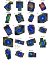 |
Fig. 1. Three-colour images for the galaxies in our sample showing a combination of Hα emission from MUSE IFS (red), 21 μm emission from JWST MIRI F2100W images (green), and stellar mass surface density from MUSE full spectral fitting (blue). The JWST data and MUSE data are shown at matched resolution. Galaxies are shown in order of increasing stellar mass. Foreground stars and the AGN in NGC 1566 and NGC 1365 are masked. The diffraction spikes due to bright AGN in NGC 4535, NGC 7496 and NGC 1365 are shown here but masked in subsequent analysis. The jagged edges of the images are caused by the intersection between the MUSE and MIRI image coverage. |
2.2. MUSE data and the optical H II region catalogue
We compareed the JWST images with maps of Hα and Hβ obtained with IFS from the PHANGS–MUSE programme (Emsellem et al. 2022), and the associated H II region masks (Groves et al. 2023). In short, individual MUSE pointings (field of view of 1′×1′) were convolved with a kernel chosen to generate a common Gaussian PSF across each galaxy mosaic which is also constant as a function of wavelength. We refer to the resulting PSF as convolved-optimised or ‘copt’. We adopted this copt FWHM as the target resolution for the JWST images, except in the case of NGC 4535 already noted above. Table 1 summarises the adopted FWHM resolution for each galaxy.
H II region masks were derived with the HIIPHOT algorithm (Thilker et al. 2000), which separates nebulae from the surrounding emission by first defining seed regions around bright peaks, and extending them until a termination gradient in the surface brightness profile is reached. Line fluxes and key nebular properties (e.g. metallicity, ionisation parameter) were derived within each H II region integrating the spectra inside the mask following the procedure detailed in Groves et al. (2023).
Fluxes in each JWST band were extracted within our H II region masks by reprojecting the convolved JWST images onto the MUSE astrometric grid. Regions only partially covered by the footprint of the MIRI data or including masked or saturated pixels were discarded. Since the MIRI and NIRCam coverage in each target is not identical, and some targets lack NIRCam data coverage, some H II regions have MIRI fluxes but lack NIRCam ones, or vice versa. In general, for each section of the analysis we used all H II regions with valid JWST data, leading to a slightly different sample of regions when different bands are considered. We have checked that restricting the analysis to H II regions that have valid fluxes in all JWST bands does not alter the results.
No local background subtraction was performed in our fiducial analysis because of the substantial crowding of sources and the resulting uncertainty intrinsic to a local background definition. However, we tested the impact of this choice by performing a simple local background subtraction for each H II region. We defined the background as the mean surface brightness in an annulus around each region two MUSE pixels (each pixel is 0.2″) distant from the region boundary and three pixels in width. If such an annulus overlapped with other regions, we removed the overlap area from the background mask. This procedure is simplistic and leads to fairly large background levels. For example, at 21 μm 25% of the H II regions in our sample have fluxes consistent with the local background with their error, and the average contrast between the flux in the H II regions and in the background is 1.5. Because of the fairly arbitrary choices involved in the definition of a background level, we focus instead on the analysis of H II region fluxes without background subtraction throughout this work, but we comment in the text and tables on the effect of the background subtraction, where relevant.
When considering the properties of H II regions we further applied cuts in the BPT (Baldwin–Phillips–Terlevich, Baldwin et al. 1981; Phillips et al. 1986) diagrams [N II]/Hα versus [O III]/Hβ and [S II]/Hα versus [O III]/Hβ, corresponding to the dividing lines of Kauffmann et al. (2003) and Kewley et al. (2001), respectively, to minimise contamination from supernova remnants and planetary nebulae (Groves et al. 2023). This excluded 25% of the starting sample of nebulae. Finally, we discarded regions overlapping with foreground stars (0.3%), or that have a signal-to-noise ratio lower than three in Hα or Hβ (0.4%). We obtained a final sample of 19 901 regions with signal-to-noise ratio larger than three in F2100W. Their distribution across the sample is summarised in Table 1.
2.3. Balmer decrement and extinction correction
The attenuation correction using the Balmer decrement was computed assuming Case B recombination, temperature T = 104 K and density ne = 102 cm−3, leading to IHα, corr/IHβ, corr = 2.86 (Osterbrock & Ferland 2006). Under these assumptions
![Mathematical equation: $$ \begin{aligned} E(B-V) = \frac{2.5}{k_{\rm H\beta } - k_{\rm H\alpha }} \log _{10} \left[\frac{L_{\rm H\alpha }/L_{\rm H\beta }}{2.86}\right], \end{aligned} $$](/articles/aa/full_html/2023/10/aa47175-23/aa47175-23-eq2.gif) (2)
(2)
where kHα and kHβ are the value of the assumed reddening curve at the wavelengths of the two emission lines. We assumed the attenuation law of O’Donnell (1994).
In order to minimise the effect of distance (and correlated distance uncertainties) across our sample, we present results for H II regions in terms of luminosity per unit area, and in the following IHα, IHα, corr and Iband refer to the luminosity per unit area of observed Hα emission, Balmer decrement corrected Hα, and one of the JWST bands, all in units of erg s−1 kpc−2.
The range of distances covered by the sample (from 5.2 to 19.6 Mpc) may affect the amount of background contamination, although within our small sample we cannot identify a distance-related change in the relations we study in the rest of this work. Values of luminosity per unit area are corrected by a factor of cos i, where i is the galaxy inclination, to account for projection effects (Lang et al. 2020, Table 1). Since our sample excludes highly inclined galaxies, not performing this correction has minimal impact on the results.
2.4. Other ancillary data
Throughout this work we use a number of additional physical quantities to characterise H II regions and their local environments. We summarise the definitions, data sets leveraged, and the publications where each of these physical quantities were first derived in Table 2.
Summary of additional data and physical quantities used in this work.
In particular, we define a specific star-formation rate (sSFR) at the location of our H II regions from the attenuation-corrected Hα assuming full sampling of the IMF, to allow for a direct comparison with the work of Belfiore et al. (2023). We define
 (3)
(3)
where CHα is the conversion factor derived for a fully sampled initial mass function (IMF) by Calzetti et al. (2007), and Σ⋆ is the stellar mass surface density estimated from the MUSE data at the location of the H II region, corrected downwards by 0.09 dex to bring it into agreement with the stellar masses obtained by Salim et al. (2018) and Leroy et al. (2019) based on SED fitting (see discussion in Belfiore et al. 2023). This stellar mass surface density estimate does not refer to the mass of the cluster ionising the H II region, which cannot be resolved in the MUSE data, but is derived in larger spatial bins, of size comparable to the copt PSF FWHM (Emsellem et al. 2022).
In addition, in Sect. 3.1.3 we use the molecular gas mass surface density, as traced by CO(2−1) maps obtained as part of the PHANGS–ALMA programme (Leroy et al. 2021a,b), at the positions of our optically defined H II regions. The ALMA data has slightly lower angular resolution than copt (∼1.3″) for each of our galaxy targets, but considering the integration over the H II region masks the small mismatch in resolution does not affect our results.
3. Results
3.1. Using 21 μm emission as a tracer of obscured star formation
We aim to provide attenuation-corrected measures of the ionising photon luminosity from massive stars to trace recent star formation in individual H II regions. To do so, we follow the well-established approach of using the MIR to correct for the obscured part of the Hα luminosity (Hirashita et al. 2003; Calzetti et al. 2007; Kennicutt et al. 2009; Belfiore et al. 2023). Taking the MIRI F2100W band centred at 21 μm as our fiducial band, we can write the attenuation-corrected Hα luminosity per unit area as
 (4)
(4)
where all luminosities are expressed in units of erg s−1 kpc−2 (i.e. I21 = ν21Iν) and a21 is a dimensionless coefficient. This coefficient is generally calibrated empirically because of its complex dependence on star-formation history, star-dust geometry, shape of the dust attenuation law, and potential non-linearity in the dust emissivity with radiation field strength. The dust attenuation at the wavelength of Hα can therefore be related to the I21/IHα ratio via
 (5)
(5)
An equivalent formalism can be used with the PAH-tracing bands (Sect. 3.2).
As a starting point for our analysis we consider the numerical value of the coefficient obtained by Calzetti et al. (2007) for a sample of star-forming complexes in nearby galaxies using Spitzer 24 μm MIPS data:  . To apply this to JWST data we take into account the different filter bandpasses between MIPS 24 μm and MIRI F2100W using the average flux ratio tabulated by Leroy et al. (2023b), ⟨I21/I24⟩ = 0.91, leading to
  .
.
3.1.1. 21 μm emission in H II regions and the diffuse component
In this section we present the relative spatial distribution of 21 μm and Hα emission. In Fig. 1 we show three-colour images combining Hα from MUSE (red) with 21 μm emission from MIRI at copt resolution (green) and stellar mass surface density from MUSE full-spectral fitting (blue). Galaxies are ordered by increasing total stellar mass. The figure highlights the variety of stellar and ISM morphologies present in our sample. Throughout the sample we observe a strong spatial correlation between bright 21 μm sources and bright Hα emission, as expected if both components are powered by young stars (and dust attenuation is moderate, see discussion in Leroy et al. 2023b). The fainter 21 μm emission outside H II regions appears filamentary, suggesting that such emission traces primarily changes in the column density of cold gas illuminated by the diffuse interstellar radiation field (Leroy et al. 2023b; Sandstrom et al. 2023b). The presence of diffuse Hα, on the other hand, correlates spatially with the positions of H II region, and can largely be attributed to leaking ionising radiation (Belfiore et al. 2022).
To discuss the relation between Hα and 21 μm emission more quantitatively we focus on one of the galaxies in our sample, NGC 628, a grand-design spiral galaxy with log(M⋆/M⊙) = 10.3. Figure 2 (top row) presents a comparison between the 21 μm and Hα maps for NGC 628 at matched (copt) resolution. To quantify the spatial differences between Hα and 21 μm emission we compute the 21 μm flux within and outside the optically defined H II region masks (blue contours in Fig. 2, bottom left). We find that in NGC 628, 54% of the 21 μm emission, but only 36% of the Hα emission, lies outside the H II region masks. Across the full sample the fraction of 21 μm flux outside H II regions is on average ∼60%. This fraction is higher than the fraction of diffuse Hα, which averages to 38%.
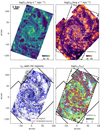 |
Fig. 2. Comparison of the Hα and 21 μm emission for NGC 0628. Top-left: 21 μm surface brightness image obtained using the F2100W filter on MIRI, convolved to the MUSE copt resolution (0.92″). Top-right: map of the Hα surface brightness from MUSE (Emsellem et al. 2022). White contours enclose regions of bright 21 μm emission (I21 > 1040.5 erg s−1 kpc−2). Bottom-left: same as top-left, but with the boundaries of the optically selected H II regions from Groves et al. (2023) in blue and the 21 μm sources which do not overlap with optical H II regions from Hassani et al. (2023) in red. Bottom-right: ratio map of the Hα to F2100W surface brightness. Red contours are bright Hα regions, IHα > 1038.8 erg s−1 kpc−2. White regions within the mapped area represent areas with S/N < 3 in F2100W. The boundaries of the MUSE (solid black) and MIRI (dashed black) mosaics are shown to aid in visualising the data overlap. |
The large amount of 21 μm emission outside H II regions is not due to a population of fully embedded star-forming regions, which may have eluded our optical catalogues. To demonstrate this, we match the MUSE H II region catalogue with the catalogue of 21 μm compact point sources from Hassani et al. (2023) for the four galaxies in common (IC 5332, NGC 628, NGC 1365, NGC 7496). For this sub-sample we identify 21 μm sources which do not overlap MUSE H II regions. We allow a maximum overlap of 10% in area and require sources to have MIR colours typical of the ISM, in order to exclude background galaxies and dusty stars (the selection criteria are discussed in Hassani et al. 2023). While the vast majority of 21 μm point sources overlap with H II regions, in NGC 628 we find 53 non-overlapping sources, accounting for 0.7% of the total 21 μm emission (shown as red circles in Fig. 2, bottom left). These sources do not overlap with supernova remnants or planetary nebulae in the Groves et al. (2023) catalogue, so we consider them likely fully embedded star-forming regions. Over the sub-sample of four galaxies in common with Hassani et al. (2023) we find that the fraction of 21 μm emission in such embedded point sources is of the order of a few percent. Their contribution is therefore negligible in explaining the diffuse 21 μm emission.
The difference in diffuse fraction between Hα and 21 μm emission implies that areas that are faint in Hα show a higher I21/IHα ratio. In the bottom-right panel of Fig. 2 we show a ratio map of I21/IHα with red contours corresponding to regions of bright Hα emission1. The higher I21/IHα in the DIG with respect to H II regions does not imply, however, that the diffuse component suffers from a higher dust attenuation, as may be expected from a naive application of Eq. (5). In fact, the 21 μm and Hα emission are powered by different components of the radiation field, and the observed change in the ratio likely reflects differences in the radiation field rather than dust attenuation. The diffuse Hα is mostly the result of the leakage of ionising photons from H II regions, with a small (few percent) contribution from old stars (Belfiore et al. 2022). The 21 μm emission, on the other hand, is powered by UV and optical light escaping star-forming regions but also originating from the old stellar population, with this ratio changing as a function of local environment (De Looze et al. 2014; Williams et al. 2019). In this work we therefore focus enitirely on the emission properties of H II regions, where both dust and Hα should be powered by the same sources. The contamination from the diffuse component is, however, likely to affect the measured properties of the fainter H II regions. A more detailed study of the diffuse IR emission and its dependence on local environment will instead be presented in a future publication. For the remainder of this work we focus on calibrating the dust correction measures for H II regions.
3.1.2. H II region scaling relations at 21 μm
We test the framework for dust attenuation correction presented in Sect. 3.1 on the scale of H II regions using the JWST F2100W band. We start by presenting the relation between the observed IHα and I21 in H II regions (Fig. 3). The two quantities show an excellent correlation. A linear fit to log quantities is performed by using the Bayesian framework described in Kelly (2007) which takes into account the errors on both variables. This leads to a sub-linear slope (0.92) and residual scatter around the best-fit relation of 0.27 dex.
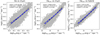 |
Fig. 3. Scaling relations between I21 and IHα for H II regions. Left: I21 as a function of IHα for the H II regions (grey points) in our sample. The white dots represent the median relation, while the blue dashed line is the best-fit power law obtained by fitting the data considering the errors associated with the quantities on both axes. The solid black line shows a linear relation normalised to match the data at high surface brightness. The slope and intercept of the best-fit power law together with the scatter with respect to the best model are reported in the top left corner. The meaning of the symbols and lines is the same across the three panels, except that the solid black line the right panel represents a one-to-one relation. Middle: I21 as a function of IHα, corr. Right: |

If one corrects the Hα emission for dust attenuation via the Balmer decrement, we obtain a relation with lower scatter (0.22 dex), but still a sub-linear slope of 0.86 (Fig. 3, middle panel). In this space, however, the best-fit relation (blue line) deviates from the observed data for regions of high surface brightness. This result may be compared with Leroy et al. (2023b), who analyse most of the area in each galaxy, therefore including diffuse emission, and obtain a slope of 0.77 (inverse of their reported slope of 1.29 fitting the IHα as a function of I21). For H II regions, at log(IHα/erg s−1 kpc−2) > 39.0 the relation approaches a linear slope (black line). Since bright H II regions also show higher values of dust attenuation, we interpret this as indicating that, when obscured SFR is dominant, both IHα, corr and I21 are good proxies for the total ionising photon production rate.
Finally, we show the relation between IHα, corr and the hybrid 21 μm and Hα tracer (Eq. (4)) using the constant  value. In this case the quantities on the two axes show correlated errors and we take the non-diagonal elements of the covariance matrix into account to perform the fit, as described in Kelly (2007). The effect of covariance between the x- and y-axes is small in our case, with an average correlation coefficient of 0.02. Performing a fit to the log quantities, we obtain a power law slope of 0.85 and scatter of the residuals of 0.10 dex. The hybrid tracer therefore provides an excellent match to the Balmer decrement-corrected Hα, but the resulting relation is still not linear. In particular, comparing the best-fit line (dashed blue) with the one-to-one line (black) the calibration leads to an overestimate of the dust correction at low Hα surface brightness and a slight underestimate for the high end.
A local background subtraction leads to relations that are closer to linear, but suffer from larger scatter (e.g. a slope of 1.03 for the relation between IHα, corr and the hybrid 21 μm and Hα, and a scatter of 0.37 dex). The deviation from linearity at low Hα surface brightness is less evident, but still present. Because of the difficulty to provide a robust measure of the background, especially for faint regions, we do not further pursue this calculation.
3.1.3. Secondary dependencies of the calibration coefficient for 21 μm emission
In this section we test whether an additional physical parameter drives the deviation from linearity observed using a constant a21 coefficient. We assume that the Balmer decrement traces dust attenuation across our sample (i.e. that we do not see any fully embedded emission) and calculate the a21 coefficient using Eq. (5). For ease of benchmarking we consider the ratio between the inferred a21 and the C07-equivalent value of  .
.
Figure 4 shows  as a function of several H II region properties derived either in this work or in Groves et al. (2023). In several of the panels in Fig. 4 the quantities on the x- and y-axis are not statistically independent. We have checked, however, that analytical propagation of the error correlations implies a degree of correlation much smaller (on average 2 dex smaller) than that observed in the data: that is to say the observed trends cannot be explained by covariance among the errors alone.
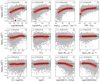 |
Fig. 4. Measured coefficient a21 normalised to the (rescaled) value from Calzetti et al. (2007) for H II regions as a function of several physical properties. Grey points are individual H II regions, while red hexagons represent the median values as a function of the quantity on the x-axis. In each panel we report the values of the Spearman rank correlation coefficient (and its error). The 16th–84th percentiles are shown as a red shaded area. The quantities considered on the x-axis are (a) equivalent width of Hα in emission, (b) sSFR surface density, defined as the ratio between the SFR surface density obtained from dust attenuation corrected Hα (assuming a fully sampled IMF) and the stellar mass surface density measured from MUSE data via spectral fitting (Σ⋆), (c) Hα luminosity per unit area corrected for dust attenuation with the Balmer decrement (IHα, corr), (d) E(B − V) of the gas obtained from the Balmer decrement, (e) ratio of the luminosity per unit area in F2100W to that in F200M (I21/I2.0), (f) luminosity per unit area in F2100W, (g) MUSE stellar mass surface density from fits to the stellar population to optical spectra, (h) molecular gas surface density, derived from ALMA CO(2−1), (i) gas-phase metallicity, (j) ionisation parameter, (k) [S II]λλ6717,31/Hα ratio, and (l) [O I] λ6300/Hα ratio. |
We quantify the correlations between each set of quantities via the Spearman rank correlation coefficient. In order to estimate the error on this statistic we perform a Monte Carlo simulation by adding Gaussian noise to the data. We take into account the correlations between the errors on the x- and y-axis by sampling from a 2D Gaussian with the appropriate covariance matrix for each data point. The median and standard deviations of 1000 Monte Carlo runs are taken as our best estimates of the Spearman rank correlation coefficient and its error, and are shown in the top-left for each panel in Fig. 4. Given the relatively high signal-to-noise ratio in H II regions and the large dynamic range spanned in most quantities with respect to their errors, the errors on the correlation coefficients are found to be small (∼0.01 in all panels).
The inferred a21 coefficient demonstrates significant positive correlations with EW(Hα) (ρ = 0.65, panel a), sSFR estimated from the attenuation-corrected Hα (ρ = 0.63, panel b), attenuation-corrected Hα surface brightness (IHα, corr, ρ = 0.60, panel c), E(B − V) computed from the Balmer decrement (ρ = 0.54, panel d), and the ratio of 21 μm to 2.0 μm surface brightness, where the surface brightness at 2.0 μm is taken from the NIRCam imaging data in the F200W filter (ρ = 0.39, panel e). EW(Hα), sSFR, and I21/I2.0 trace the luminosity of the H II region with respect to that of the old stars. E(B − V) is known to correlate with both attenuation-corrected Hα (e.g. Emsellem et al. 2022), and EW(Hα) (Groves et al. 2023). Overall, these trends suggest that a21 is slightly higher than the Calzetti et al. (2007) value for the brightest (and dustiest H II regions), while it should be significantly lower, by up to 1.0 dex for faint, less dusty regions. All these correlations flatten for the brightest H II regions.
Substantially weaker correlations (with |ρ|< 0.3) are found as a function of galactrocentric radius (panel f), stellar mass surface density (panel g), molecular gas surface density (panel h), gas-phase metallicity (panel i), or ionisation parameter (the ratio between the ionising photon flux and the hydrogen density in H II regions, panel j).
Finally, the relation between a21 and [S II] λλ6717,31/Hα (panel k) or [O I] λ6300/Hα (panel l) is flat at low values of these line ratios, but shows a strong negative correlation (ρ = −0.46 and ρ = −0.45, respectively) for higher ones. These line ratios have been studied in our sample by Belfiore et al. (2022) and are found to increase with decreasing Hα surface brightness, corresponding to the transition between H II regions and diffuse ionised gas (Haffner et al. 2009; Zhang et al. 2017). Even though we are focusing on H II regions here, we are likely seeing the increased contribution of the diffuse ionised gas background to the flux within the masks corresponding to faint H II regions going hand in hand with an increase in the relative significance of the 21 μm background. We have tested the effect of defining a local background subtraction, which leads to an increase in the scatter and a decrease in the strength of all correlation coefficients, but does not change the shape and sign of the strongest ones.
3.2. Using PAH-tracing bands to measure obscured star formation
In this section we test the ability of PAH-dominated bands to trace the obscured component of star formation. We consider the continuum-subtracted F335M NIRCam band (F335MPAH), and the MIRI bands centred at 7.7 μm (F770W), 10 μm (F1000W), and 11.3 μm (F1130W). Emission in the 7.7 μm and 11.3 μm bands is dominated by features generally associated with PAHs (Smith et al. 2007; Draine & Li 2007), while the star-light contamination in the F335M band is removed as described in Sect. 2.1 and Sandstrom et al. (2023b). The nature of the continuum emission underlying the PAH features and dominating the 10 μm band emission remains unclear (Smith et al. 2007; Li 2020). Leroy et al. (2023b) find that the 10 μm continuum closely follows the PAH-dominated bands, rather than the 21 μm emission. In this work we therefore refer collectively to F335MPAH, F770W, F1000W, and F1130W as ‘PAH-tracing’ bands.
3.2.1. PAH-tracing band ratios in H II regions
We adopt an empirical strategy to set fiducial values of the hybridisation coefficients for each band, aband. We calculate these coefficients, which we refer to as ‘C07-equivalent’, by scaling the value of the Calzetti et al. (2007) 21 μm coefficient using the average band ratio between PAH-tracing bands and F2100W. In detail, we define
 (6)
(6)
where ⟨log(Iband/I21)⟩ is the median band ratio between the bands of interest (3.3, 7.7, 10, and 11.3 μm) and 21 μm in our H II region sample. We report the median, 16th, and 84th percentiles of the distribution of Iband/I21 in Table 3. The scatter in the Iband/I21 lies in the range of 0.2 dex (F770W) to 0.4 dex (F335MPAH). Part of this larger scatter for F335MPAH may be attributed to residuals in the continuum subtraction.
Median (and 16th and 84th percentiles) of the ratio between the F335MPAH, F770W, F1000W, F1130W to the F2100W luminosity (in units of erg s−1 kpc−2) for the H II regions in our sample.
3.2.2. H II region scaling relations for PAH-tracing bands
Figure 5 shows the relations between Hα corrected using the Balmer decrement and the Hα hybridised with each of the PAH-dominated bands using the  factor defined in Eq. (6). For all bands considered we obtain a best-fit power law with sub-linear slopes (ranging from 0.82 to 0.89) and ∼0.10 dex scatter (except for F335MPAH for which we obtain a marginally larger scatter of 0.13 dex).
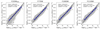 |
Fig. 5. Comparison of Hα hybridised with F335MPAH, F770W, F1000W and F1130W and the attenuation-corrected Hα obtained using the Balmer decrement. The dashed blue line is the best linear fit while the white circles represent a binned average. The slope and intercept of the best-fit power law together with the scatter with respect to the best model are reported on the top left corner. The solid black line represents the one-to-one relation. |
These results are remarkably consistent with those obtained with F2100W in Sect. 3.1.2. In fact, Fig. 5 demonstrates that the hybrid recipe overestimates the dust correction at low surface brightness levels (log(IHα, corr/erg s−1 kpc−2) < 39), while underestimating it at high surface brightness levels, as already observed for F2100W.
3.2.3. Secondary relations of aband for PAH-tracing bands
In Fig. 6 we show the median trends of the aband coefficients for different bands as a function of EW(Hα). The values of aband are scaled logarithmically and normalised, so that the zero on the y-axis corresponds to the C07-equivalent value. The trend for F2100W (purple) was already presented in Fig. 4, but here we compare it directly with the behaviour of the other bands. For log EW(Hα)/Å < 1.5 (or log(sSFR/yr−1) < − 10) all bands follow a closely matching trend of increasing aband with EW(Hα), reaching the C07-equivalent value at log EW(Hα)/Å ∼ 1.5.
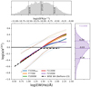 |
Fig. 6. log aband normalised to the C07-equivalent values as a function of EW(Hα) and sSFR (alternative x-axis on top) for H II regions in our sample, where band = [F335MPAH (blue), F770W (orange), F1000W (green), F1130W (red), F2100W (purple)]. The coloured solid lines represent the median relations, while the coloured dashed lines show the 16th and 84th percentiles of the distribution. The black dashed line is the best-fit to the low-resolution (kpc-scale) Hα + WISE W4 data from Belfiore et al. (2023). The grey histogram (top) shows the distribution of EW(Hα) in the H II regions used in this work (with 16th, 50th, 84th percentiles marked and labelled). The purple histogram (right) shows the distribution of |

At high EW(Hα), on the other hand, the behaviour of different bands diverges. The dependence of a21 on EW(Hα) flattens for log EW(Hα)/Å > 2, plateauing to a constant value of a21 that is 0.16 dex higher than the C07-equivalent one. The F335MPAH band also shows a flattening in the slope of the relation but with no plateau, while F770W, F1000W, and F1130W follow increasing trends.
The difference between the PAH-tracing bands reflects the relative brightness of different features in the MIR spectrum. For example, Chastenet et al. (2023a) find that the ratio of (I7.7 + I11.3)/I21, which traces PAH abundance (Draine et al. 2021), is relatively constant in the diffuse ISM, but decreases in bright H II regions. Egorov et al. (2023) find that this ratio in H II regions anti-correlates with the ionisation parameter, which is tracing the density of the extreme UV photons in the region. Moreover, Chastenet et al. (2023b) find that the F335MPAH band is enhanced and the F1130W band is suppressed in regions of high Hα surface brightness. These trends indicate that the abundance of PAHs is lowered in H II regions, due to their destruction by extreme UV photons, but also imply changes in the average properties of the PAH population, namely a decrease in average size and an increased abundance of charged grains and/or hotter grains.
We show the change in the Iband/I21 ratios as a function of EW(Hα) in Fig. 7. The ratio for each band is normalised by subtracting the median value for the sample, allowing for easier comparison of the trend across bands. Figure 7 shows the expected decrease in the ratios of I7.7/I21, I10/I21, and I11.3/I21 as a function of EW(Hα). I7.7/I21 shows a slightly shallower slope than I10/I21 and I11.3/I21. The I3.3/I21 ratio, on the other hand, shows a much flatter (and even increasing) trend.
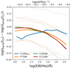 |
Fig. 7. Ratio of Iband/I21 normalised to the sample mean (⟨Iband/I21⟩) as a function of EW(Hα), for band = [F335MPAH (blue), F770W (orange), F1000W (green), F1130W (red)]. The solid lines represent the median, while the dashed lines correspond to the 16th and 84th percentiles. The alternative x-axis on top shows the sSFR associated with each EW(Hα) value. The median trends show that I3.3/I21 does not show the same decrease with EW(Hα) as the ratios of the other PAH bands. |
Finally, our targets are relatively metal-rich, so we do not probe the low-metallicity regime typical of dwarf galaxies where the PAH fraction is observed to be lower (Madden et al. 2006; Draine & Li 2007; Khramtsova et al. 2013). Previous work, however, focused on studying entire galaxies or kpc-size regions. On the scale of H II regions in our metallicity range the PAH fraction is found not to depend on metallicity (Egorov et al. 2023), but rather on the intensity of hydrogen-ionising radiation that probably regulates the PAH destruction in H II regions. Overall EW(Hα) remains the most significant secondary correlation for the PAH bands, and we therefore do not consider additional ones in this work.
4. Discussion
This work presents an unprecedented set of resolved IR data for star-forming regions at ∼100 pc scales. Our results show the promise, and caveats, involved in the use of hybrid SFR indicators on the scales of H II regions. In particular, we use IR observations with JWST at 3.3, 7.7, 10, 11.3, and 21 μm to correct Hα emission from H II regions for dust attenuation using a hybrid recipe. Using a scaled version of the C07 coefficient (Eq. (6)) leads to hybrid SFR estimations which agree with the SFR derived via the Balmer decrement to within ∼0.1 dex, but show systematic deviations for both low and high SFR. These deviations correlate most notably with quantities tracing sSFR (e.g. EW(Hα)).
4.1. Recommendation for using constant aband
We report in Table 4 the median values of the aband coefficients for our full sample of 19 901 H II regions, together with the C07-equivalent values. Our median aband are in excellent agreement with the C07-equivalent values, but the scatter around these values (quantified as the 16th and 84th percentiles) are large.
Hybridisation coefficients for various JWST bands.
In Table 4 we also present the median values of the aband coefficients after performing a local background subtraction. These values are ∼0.2 to 0.4 dex larger than our nominal ones. The background subtraction more strongly affects the F770W, F1000W, and F1130W bands (a increases by ∼0.4 dex), while it has a smaller effect on F2100W and F335MPAH (a increases by ∼0.2 dex).
The agreement between our values and the C07-equivalent ones is not immediately expected. Calzetti et al. (2007) estimate the background in large sub-galactic regions, but not using local annuli, therefore likely resulting in an intermediate estimate of the value of the background level. However, the median aband will also depend on the distribution of EW(Hα) in the sample of regions considered and on the median spatial resolution.
In fact, Fig. 6 demonstrates that the plateau observed using kpc-resolution IR data (WISE 22 μm in Belfiore et al. 2023) is a resolution effect, due to the blending of different H II regions with each other and with the diffuse medium. The trend observed by Belfiore et al. (2023) using kpc, 15″-resolution WISE W4 22 μm data and the full PHANGS–MUSE galaxy sample, is shown as the black dashed line in Fig. 6. JWST F2100W observations, providing a factor of ∼15 higher spatial resolution than WISE W4, reveal that the relation between a21 and EW(Hα) plateaus at higher EW(Hα) (and a21) than seen in the low-resolution data. Since our observations resolve the inter-cloud distance (∼100 pc, Kim et al. 2022), and the contamination from the diffuse background is minimal for the bright regions, we expect the trend uncovered by JWST to persist at even higher spatial resolution. This hypothesis can be tested with upcoming JWST observations of more nearby (or Local Group) galaxies.
Finally, we note that our background subtraction strategy does not remove the trend of increasing aband with EW(Hα). Future work may consider more advanced approaches to model the background and test whether such contamination can explain the behaviour observed in Fig. 6 at low EW(Hα).
4.2. Modelling the impact of old stellar population on aband
The trend of increasing aband with EW(Hα) likely reflects the increasing contribution from dust heated by old stellar populations in fainter regions (Cortese et al. 2008; Leroy et al. 2012; Boquien et al. 2016; Nersesian et al. 2019), and, for the PAH-tracing bands, the roughly constant band ratios in diffuse regions (Chastenet et al. 2019).
Modelling the behaviour of aband as a function of EW(Hα), or one of the other parameters studied in Sect. 3.1.3, would provide a more accurate estimate of the dust-attenuated star formation, and a prescription more readily applicable to lower-resolution data. Several authors have presented calibrations including such additional terms, for example colours, sSFR, or M⋆ (Boquien et al. 2016; Zhang & Ho 2023; Belfiore et al. 2023; Kouroumpatzakis et al. 2023).
We aim to provide such a second-order correction applicable to nearby galaxies data. The functional form that this correction should take is not evident a priori. For the sake of simplicity, here we add an additional linear term to the conventional hybrid star formation recipe presented in Eq. (4), leading to
 (7)
(7)
where IIR is one of the JWST IR dust-tracing bands, and IQ is a second physical quantity appropriately chosen to best reproduce the extinction correction from the Balmer decrement. As before, we express all surface brightness measurements in units of erg s−1 kpc−2.
We first consider the task of deriving an estimate for the obscured SFR using two JWST bands: a dust-tracing band (F2100W or any of the PAH-tracing bands), and a second band tracing stellar continuum emission (F200W, F300M or F360M) to account for the dust heating from old stars. To determine the best combination of bands for such a calibration we ran a random forest regression, using the algorithm implementation in SCIKIT-LEARN (Pedregosa et al. 2011). In particular, we used the random forest model to determine the relative importance of input features (Bluck et al. 2022; Baker et al. 2022). This approach is conceptually similar to more traditional principal component analysis, but allows the generation of more complex, non-linear models.
The random forest algorithm is a form of supervised machine learning that builds a non-parametric model using multiple decision trees, trained to decrease the mean square error at each split. We used E(B − V) as the target variable since the goal is to understand how best to perform the dust correction, and Iband/IHα, where ‘band’ is one of the JWST bands available to us (F200W, F300M, F360M, F335MPAH, F770W, F1000W, F1130W, F2100W), as input features. We also considered an array of random numbers as an additional input feature to test the performance of the algorithm. The dataset was subdivided into a training (80% of the full sample) and testing (remaining 20%) subset of H II regions. Only H II regions covered by both NIRCam and MIRI and with signal-to-noise ratio grater than 3 in all JWST bands were used for this computation. After training, the mean square error (MSE) of the test set was compared with that of the training sample in order to check the quality of the resulting model and avoid overfitting.
We found that the combination of I21/IHα and I2.0/IHα accounts for nearly all the variance in E(B − V) (Fig. 8). Once these two variables are taken into account, the remaining ones have residual importance consistent with random within the errors. The MSE of the training and test set are comparable (reported on the top right of Fig. 8), demonstrating that the algorithm produced a successful model. This analysis confirms two of the key insights from this work: (1) F2100W is the best band to use for hybridisation among the bands tracing dust emission available in our PHANGS–JWST filter set, and (2) there exists an evident secondary dependence on the stellar mass-tracing NIRCam bands, of which the best is F200W.
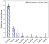 |
Fig. 8. Relative importance of different band ratios in predicting the E(B − V) of H II regions using a random forest model. The error-bars are obtained by bootstrap random sampling. The mean squared errors (MSE) are shown for both the testing and the training set. I21/IHα and I2.0/IHα account for most of the variance in the data. |
Having established I21 and I2.0 as the two best variables, we fitted the extinction-corrected Hα surface brightness with a two-parameter regression model, using the Bayesian formalism discussed in Hogg et al. (2010). We fitted for the α and β parameters in Eq. (7) and for intrinsic scatter in the relation, using the Bayesian Monte Carlo sampler EMCEE, and obtained best-fit as relation
 (8)
(8)
We also fitted using the F300M and F360M NIRCam bands, obtaining α = 0.025, β = 8 × 10⁻⁴ and α = 0.025, β = 7 × 10⁻⁴, respectively.
Our approach here is similar to the one of Kouroumpatzakis et al. (2023), who used spectral energy distribution models generated with the code CIGALE to study how best to determine SFR from JWST bands. In their work, however, Kouroumpatzakis et al. (2023) did not consider IHα, but modelled the SFR as a linear combination of I21 and I2.0. Their results are therefore not directly comparable. We leave a direct comparison of our results with spectral energy distribution models to future work.
Finally, we repeated our two-parameter fit using stellar mass surface density Σ⋆, which may be used in the absence of JWST NIRCam data. We obtained
 (9)
(9)
where surface brightnesses are in units of erg−1 s−1 kpc−2 and Σ⋆ is in units of M⊙ kpc−2.
4.3. IR emission as a tracer embedded SFR or cold gas
The MIR, and in particular the bands containing strong PAH features, show excellent correlations with the cold molecular gas content, mapped by CO emission (Regan et al. 2006; Chown et al. 2021; Whitcomb et al. 2023; Leroy et al. 2023a). Leroy et al. (2021b, 2023a), for example, found a nearly linear relation between the intensity in the WISE W3 band centred at 12 μm and CO(2−1) emission. This correlation was found to have lower scatter than that between CO and IR emission at ∼24 μm. Whitcomb et al. (2023) similarly argued using correlation analysis that emission around 12 μm traces CO emission better than SFR, while IR emission at 24 μm traces SFR better than CO. Leroy et al. (2023b) used the early JWST data for four galaxies from our sample and compare the MIR emission with both Hα and CO emission, finding that MIR emission correlates well with both extinction-corrected Hα and CO. Such a result is expected, since dust emission depends on both the dust surface density and the intensity of the radiation field heating it. The convolution of these effects leads to MIR emission being a useful tracer of both IHα, corr and CO.
Within H II regions, however, one expects a tighter relation between MIR emission and star formation than between MIR emission and cold gas content. To test this hypothesis we evaluated the relative ability of each of the JWST bands considered in this work to trace extinction-corrected Hα, molecular gas (as traced by CO(2−1)), and stellar mass surface density, focusing our analysis on H II regions specifically. The analysis was performed by building a random forest regression model for the surface brightness in each JWST band and using IHα, corr, ICO, and Σ⋆, in addition to a vector of random numbers, as input features. The relative importance of each of the features in reproducing the brightness in each JWST band considered is presented in Fig. 9.
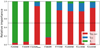 |
Fig. 9. Relative importance of extinction-corrected Hα (IHα, corr), CO(2−1) surface density, and stellar mass surface density (Σ⋆) in predicting the surface brightness of H II regions in a set of JWST bands. |
As expected, both F300M and F200W trace mostly stellar mass surface density (importance ∼90%). For F360M Hα takes up part of the importance, probably reflecting the increasing importance of hot dust and residual contamination from PAHs in this band (Sandstrom et al. 2023a). F335MPAH mostly traces Hα, highlighting the success of the continuum subtraction strategy for this band. The MIR bands trace mostly Hα, but with 20% importance attributed also to CO for F770W, F1000W, F1130W. The contribution of stellar mass is small, and it is largest at F1000W, where is amounts to 5% of the overall importance. This band contains the largest contamination from point sources, potentially evolved stars, whose density correlates with the overall stellar mass surface density. For the canonical F2100W band the relative importance of Hα and CO are 83% and 16%, respectively. In summary, both 3.3 μm and the MIR bands trace mostly extinction-corrected Hα within H II regions, with a smaller (< 20%) secondary dependence on molecular gas, as traced by CO. The small dependence on CO is consistent with the finding that many H II regions exists without associated molecular gas, in the sense of gas within the H II region boundary (Zakardjian et al. 2023). These conclusions are likely to differ within the more diffuse medium, where the relative importance of CO in determining the MIR emission is expected to increase (Leroy et al. 2023b), but we leave an exploration of these trends to future work.
5. Conclusions
We use NIRCam and MIRI images in combination with IFS from MUSE for 19 nearby galaxies to calibrate hybrid recipes to correct Hα for dust extinction on the scales of individual H II regions (∼100 pc). We examine hybrid recipes that consider a linear combination of Hα with the F2100W MIRI band, dominated by emission from small grains, and bands tracing PAH emission, namely the continuum-subtracted NIRCam F335M band (F335MPAH), and the F770W, F1000W, and F1130W MIRI bands. We summarise our main results below.
-
The ratio between 21 μm and Hα emission is systematically higher in the diffuse ISM, outside optically defined H II regions. This fact reflects a change in the dominant source of dust heating – young stars in H II regions and the old stellar population in the DIG – and not an increase in dust attenuation. Fully embedded regions make a negligible contribution to the diffuse 21 μm emission.
-
Focusing on H II regions, we calibrate the coefficient in front of the IR emission term (IHα, corr = IHα + aband Iband) by benchmarking the hybrid dust correction recipe with the correction obtained using the Balmer decrement measured from the MUSE data. We adopt fiducial hybridisation coefficients for the different dust-tracing JWST bands (
 ) by rescaling the coefficient derived by Calzetti et al. (2007) for Spitzer 24 μm emission by the average band ratio ⟨I24/Iband⟩. These C07-equivalent coefficients are in good general agreement with the median of the measured aband coefficient across our sample of H II regions for all bands considered (F335MPAH, F770W, F1000W, F1130W, F2100W). A local background subtraction causes an increase of the coefficients associated with F770W, F1000W, and F1130W bands of ∼0.4 dex, while it has a smaller effect on F2100W and F335MPAH (a increases by ∼0.2 dex). Our recommended coefficients are summarised in Table 4.
 -
For both 21 μm and the PAH-tracing bands, using a hybrid recipe with a constant coefficient
 leads to extinction-corrected Hα fluxes that correlate well (scatter ∼0.1 dex), albeit sub-linearly (slope 0.82−0.89), with those inferred from the Balmer decrement. The sub-linear slope implies that a constant aband overestimates the dust correction for faint H II regions, and it underestimates it for bright regions.
 -
We tested for secondary dependencies of aband on a number of additional physical parameters. The strongest correlations are with physical parameters that trace the ratio between young and old stellar components, for example EW(Hα), sSFR, or indirectly correlate with them (e.g. Hα surface brightness, or dust attenuation measured from the Balmer decrement). Strong correlations are also found with line ratios that trace the change in the ionisation condition between H II regions and DIG ([O I]/Hα, [S II]/Hα). These trends indicate that dust heating from the old stellar component contributes substantially to the IR emission for the fainter H II regions in our sample.
-
aband correlates with EW(Hα) for all bands considered. For EW(Hα) < 30 Å, the trends are similar for all bands and agree with the recent kpc-resolution study of Belfiore et al. (2023). At higher EW(Hα), a21 plateaus to a constant value, while the coefficients for the F770W, F1000W, and F1130W keep increasing. The behaviour of the MIR PAH-tracing bands reflects the relative decrease in PAH emission in bright H II regions, in agreement with the literature predicting the destruction of PAH molecules in such harsh environments. The F335MPAH shows an intermediate behaviour between F2100W and the other MIR bands, which can be explained by the relative increase in 3.3 μm emission with respect to the other PAH-tracing bands in H II regions, possibly tracing a decrease in the average size of PAH grains or an increase in the hardness of the UV radiation field.
-
A random forest analysis confirms that F2100W is the preferred band to consider in combination with Hα to infer dust attenuation, confirming results from previous literature using WISE 22 μm or Spitzer 24 μm bands.
-
The main secondary dependence of aband can be modelled by explicitly adding an additional linear term proportional to stellar mass surface density or 2 μm emission to the hybrid recipe. We provide coefficients for these corrections in Eqs. (8) and (9).
-
Finally, we analyse the relative importance of molecular gas (traced by CO(2−1)), stellar mass surface density, and extinction-corrected Hα in determining the surface brightness for H II regions within our JWST bands. The MIR bands trace mostly Hα, but with a smaller (15−20%) importance attributed to CO.
The analysis presented in this work extends the validity of previous widely used hybrid SFR calibrations to the ∼100 pc scale and demonstrates the transformational ability of JWST to unveil the dust-obscured component of star formation in galaxies.
log(IHα/erg s−1 kpc−2) > 38.8, chosen to correspond to the 16th percentile of the surface brightness distribution of H II regions in the PHANGS-MUSE sample from Belfiore et al. (2022).
Acknowledgments
This work is carried out as part of the PHANGS Collaboration. Based on observations made with the NASA/ESA/CSA JWST. The data were obtained from the Mikulski Archive for Space Telescopes at the Space Telescope Science Institute, which is operated by the Association of Universities for Research in Astronomy, Inc., under NASA contract NAS 5-03127. The observations are associated with JWST programme 2107 (PI: J. Lee) based on observations collected at the European Southern Observatory under ESO programmes 094.C-0623 (PI: Kreckel), 095.C-0473, 098.C-0484 (PI: Blanc), 1100.B-0651 (PHANGS-MUSE; PI: Schinnerer), as well as 094.B-0321 (MAGNUM; PI: Marconi), 099.B-0242, 0100.B-0116, 098.B-0551 (MAD; PI: Carollo) and 097.B-0640 (TIMER; PI: Gadotti). F.B. acknowledges support from the INAF Fundamental Astrophysics programme 2022. M.B. acknowledges support from FONDECYT regular grant 1211000 and by the ANID BASAL project FB210003. H.A.P. acknowledges support by the National Science and Technology Council of Taiwan under grant 110-2112-M-032-020-MY3. J.M.D.K. gratefully acknowledges funding from the ERC under the European Union’s Horizon 2020 research and innovation programme via the ERC Starting Grant MUSTANG (grant number 714907). COOL Research DAO is a Decentralized Autonomous Organization supporting research in astrophysics aimed at uncovering our cosmic origins. M.C. gratefully acknowledges funding from the DFG through an Emmy Noether Research Group (grant number CH2137/1-1). R.S.K. and S.C.O.G. acknowledge financial support from the ERC via the ERC Synergy Grant ‘ECOGAL’ (project ID 855130), from the German Excellence Strategy via the Heidelberg Cluster of Excellence (EXC 2181 – 390900948) ‘STRUCTURES’, and from the German Ministry for Economic Affairs and Climate Action in project ‘MAINN’ (funding ID 50OO2206). R.S.K. also thanks for computing resources provided bwHPC and DFG through grant INST 35/1134-1 FUGG and for data storage at SDS@hd through grant INST 35/1314-1 FUGG. J.C. acknowledges support from ERC starting grant #851622 DustOrigin. M.Q. acknowledges support from the Spanish grant PID2019-106027GA-C44, funded by MCIN/AEI/10.13039/501100011033. K.K., O.V.E. and E.J.W. gratefully acknowledge funding from the Deutsche Forschungsgemeinschaft (DFG, German Research Foundation) in the form of an Emmy Noether Research Group (grant number KR4598/2-1, PI: Kreckel). J.N. acknowledges funding from the European Research Council (ERC) under the European Union’s Horizon 2020 research and innovation programe (grant agreement No. 694343). E.R. and H.H. acknowledge the support of the Natural Sciences and Engineering Research Council of Canada (NSERC), funding reference number RGPIN-2022-03499, and the support of the Canadian Space Agency (22ASTALBER). A.K.L. gratefully acknowledges support by grants 1653300 and 2205628 from the National Science Foundation, by award JWST-GO-02107.009-A, and by a Humboldt Research Award from the Alexander von Humboldt Foundation. K.S. acknowledges funding support from grant support by JWST-GO-02107.006-A.
References
- Anand, G. S., Lee, J. C., Van Dyk, S. D., et al. 2021, MNRAS, 501, 3621 [Google Scholar]
- Aniano, G., Draine, B. T., Gordon, K. D., & Sandstrom, K. 2011, PASP, 123, 1218 [Google Scholar]
- Baker, W. M., Maiolino, R., Bluck, A. F. L., et al. 2022, MNRAS, 510, 3622 [NASA ADS] [CrossRef] [Google Scholar]
- Baldwin, J. A., Phillips, M. M., & Terlevich, R. 1981, PASP, 93, 5 [Google Scholar]
- Belfiore, F., Santoro, F., Groves, B., et al. 2022, A&A, 659, A26 [NASA ADS] [CrossRef] [EDP Sciences] [Google Scholar]
- Belfiore, F., Leroy, A., Sun, J., et al. 2023, A&A, 670, A67 [NASA ADS] [CrossRef] [EDP Sciences] [Google Scholar]
- Bendo, G. J., Dale, D. A., Draine, B. T., et al. 2006, ApJ, 652, 283 [NASA ADS] [CrossRef] [Google Scholar]
- Bendo, G. J., Boselli, A., Dariush, A., et al. 2012, MNRAS, 419, 1833 [NASA ADS] [CrossRef] [Google Scholar]
- Bluck, A. F., Maiolino, R., Brownson, S., et al. 2022, A&A, 659, A160 [NASA ADS] [CrossRef] [EDP Sciences] [Google Scholar]
- Bolatto, A. D., Simon, J. D., Stanimirović, S., et al. 2007, ApJ, 655, 212 [NASA ADS] [CrossRef] [Google Scholar]
- Bolatto, A. D., Wolfire, M., & Leroy, A. K. 2013, ARA&A, 51, 207 [CrossRef] [Google Scholar]
- Boquien, M., Kennicutt, R., Calzetti, D., et al. 2016, A&A, 591, A6 [NASA ADS] [CrossRef] [EDP Sciences] [Google Scholar]
- Calzetti, D. 2020, Nat. Astron., 4, 437 [Google Scholar]
- Calzetti, D., Kennicutt, R. C., Engelbracht, C. W., et al. 2007, ApJ, 666, 870 [Google Scholar]
- Catalán-Torrecilla, C., Gil de Paz, A., Castillo-Morales, A., et al. 2015, A&A, 584, A87 [NASA ADS] [CrossRef] [EDP Sciences] [Google Scholar]
- Chastenet, J., Sandstrom, K., Chiang, I.-D., et al. 2019, ApJ, 876, 62 [NASA ADS] [CrossRef] [Google Scholar]
- Chastenet, J., Sutter, J., Sandstrom, K., et al. 2023a, ApJ, 944, L11 [NASA ADS] [CrossRef] [Google Scholar]
- Chastenet, J., Sutter, J., Sandstrom, K., et al. 2023b, ApJ, 944, L12 [NASA ADS] [CrossRef] [Google Scholar]
- Chown, R., Li, C., Parker, L., et al. 2021, MNRAS, 500, 1261 [Google Scholar]
- Cortese, L., Boselli, A., Franzetti, P., et al. 2008, MNRAS, 386, 1157 [NASA ADS] [CrossRef] [Google Scholar]
- Crocker, A. F., Calzetti, D., Thilker, D. A., et al. 2013, ApJ, 762, 79 [NASA ADS] [CrossRef] [Google Scholar]
- De Looze, I., Fritz, J., Baes, M., et al. 2014, A&A, 571, A69 [NASA ADS] [CrossRef] [EDP Sciences] [Google Scholar]
- Den Brok, J. S., Chatzigiannakis, D., Bigiel, F., et al. 2021, MNRAS, 504, 3221 [NASA ADS] [CrossRef] [Google Scholar]
- Diaz, A. I., Terlevich, E., Vflchez, J. M., et al. 1991, MNRAS, 253, 245 [NASA ADS] [CrossRef] [Google Scholar]
- Draine, B. T., & Li, A. 2007, ApJ, 657, 810 [CrossRef] [Google Scholar]
- Draine, B. T., Li, A., Hensley, B. S., et al. 2021, ApJ, 917, 3 [CrossRef] [Google Scholar]
- Egorov, O. V., Kreckel, K., Sandstrom, K. M., et al. 2023, ApJ, 944, L16 [NASA ADS] [CrossRef] [Google Scholar]
- Emsellem, E., Schinnerer, E., Santoro, F., et al. 2022, A&A, 659, A191 [NASA ADS] [CrossRef] [EDP Sciences] [Google Scholar]
- Galliano, F., Galametz, M., & Jones, A. P. 2018, ARA&A, 56, 673 [Google Scholar]
- Groves, B., Krause, O., Sandstrom, K., et al. 2012, MNRAS, 426, 892 [NASA ADS] [CrossRef] [Google Scholar]
- Groves, B., Kreckel, K., Santoro, F., et al. 2023, MNRAS, 520, 4902 [Google Scholar]
- Gruppioni, C., Pozzi, F., Rodighiero, G., et al. 2013, MNRAS, 432, 23 [Google Scholar]
- Haffner, L. M., Dettmar, R.-J. J., Beckman, J. E., et al. 2009, Rev. Mod. Phys., 81, 969 [CrossRef] [Google Scholar]
- Hao, C. N., Kennicutt, R. C., Johnson, B. D., et al. 2011, ApJ, 741, 124 [NASA ADS] [CrossRef] [Google Scholar]
- Hassani, H., Rosolowsky, E., Leroy, A. K., et al. 2023, ApJ, 944, L21 [NASA ADS] [CrossRef] [Google Scholar]
- Helou, G., Roussel, H., Appleton, P., et al. 2004, ApJS, 154, 253 [NASA ADS] [CrossRef] [Google Scholar]
- Hirashita, H., Buat, V., & Inoue, A. K. 2003, A&A, 410, 83 [NASA ADS] [CrossRef] [EDP Sciences] [Google Scholar]
- Hogg, D. W., Bovy, J., & Lang, D. 2010, ArXiv e-prints [arXiv:1008.4686] [Google Scholar]
- Jarrett, T. H., Masci, F., Tsai, C. W., et al. 2013, AJ, 145, 6 [Google Scholar]
- Kauffmann, G., Heckman, T. M., Tremonti, C., et al. 2003, MNRAS, 346, 1055 [Google Scholar]
- Kelly, B. C. 2007, ApJ, 665, 1489 [Google Scholar]
- Kennicutt, R. C. 1998, ARA&A, 36, 189 [NASA ADS] [CrossRef] [Google Scholar]
- Kennicutt, R. C., & Evans, N. J. 2012, ARA&A, 50, 531 [NASA ADS] [CrossRef] [Google Scholar]
- Kennicutt, R. C., Calzetti, D., Walter, F., et al. 2007, ApJ, 671, 333 [NASA ADS] [CrossRef] [Google Scholar]
- Kennicutt, R. C., Hao, C. N., Calzetti, D., et al. 2009, ApJ, 703, 1672 [NASA ADS] [CrossRef] [Google Scholar]
- Kewley, L. J., Dopita, M. A., Sutherland, R. S., Heisler, C. A., & Trevena, J. 2001, ApJ, 556, 121 [Google Scholar]
- Khramtsova, M. S., Wiebe, D. S., Boley, P. A., & Pavlyuchenkov, Y. N. 2013, MNRAS, 431, 2006 [NASA ADS] [CrossRef] [Google Scholar]
- Kim, J., Chevance, M., Kruijssen, J. M. D., et al. 2022, MNRAS, 516, 3006 [NASA ADS] [CrossRef] [Google Scholar]
- Kouroumpatzakis, K., Zezas, A., Kyritsis, E., Salim, S., & Svoboda, J. 2023, A&A, 673, A16 [NASA ADS] [CrossRef] [EDP Sciences] [Google Scholar]
- Lai, T. S.-Y., Smith, J. D. T., Baba, S., Spoon, H. W. W., & Imanishi, M. 2020, ApJ, 905, 55 [NASA ADS] [CrossRef] [Google Scholar]
- Lang, P., Meidt, S. E., Rosolowsky, E., et al. 2020, ApJ, 897, 122 [CrossRef] [Google Scholar]
- Lebouteiller, V., Bernard-Salas, J., Whelan, D. G., et al. 2011, ApJ, 728, 45 [CrossRef] [Google Scholar]
- Lee, J. C., Sandstrom, K. M., Leroy, A. K., et al. 2023, ApJ, 944, L17 [NASA ADS] [CrossRef] [Google Scholar]
- Leroy, A. K., Bigiel, F., de Blok, W. J. G., et al. 2012, AJ, 144, 3 [Google Scholar]
- Leroy, A. K., Sandstrom, K. M., Lang, D., et al. 2019, ApJS, 244, 24 [Google Scholar]
- Leroy, A. K., Hughes, A., Liu, D., et al. 2021a, ApJS, 255, 19 [NASA ADS] [CrossRef] [Google Scholar]
- Leroy, A. K., Schinnerer, E., Hughes, A., et al. 2021b, ApJS, 257, 43 [NASA ADS] [CrossRef] [Google Scholar]
- Leroy, A. K., Bolatto, A. D., Sandstrom, K., et al. 2023a, ApJ, 944, L10 [NASA ADS] [CrossRef] [Google Scholar]
- Leroy, A. K., Sandstrom, K., Rosolowsky, E., et al. 2023b, ApJ, 944, L9 [NASA ADS] [CrossRef] [Google Scholar]
- Leslie, S. K., Schinnerer, E., Groves, B., et al. 2018, A&A, 616, A157 [NASA ADS] [CrossRef] [EDP Sciences] [Google Scholar]
- Li, A. 2020, Nat. Astron., 4, 339 [CrossRef] [Google Scholar]
- Lu, Y., Blanc, G. A., & Benson, A. 2015, ApJ, 808, 129 [NASA ADS] [CrossRef] [Google Scholar]
- Lutz, D., Valiante, E., Sturm, E., et al. 2005, ApJ, 625, L83 [NASA ADS] [CrossRef] [Google Scholar]
- Madau, P., & Dickinson, M. 2014, ARA&A, 52, 415 [Google Scholar]
- Madden, S. C., Galliano, F., Jones, A. P., & Sauvage, M. 2006, A&A, 446, 877 [NASA ADS] [CrossRef] [EDP Sciences] [Google Scholar]
- Maragkoudakis, A., Ivkovich, N., Peeters, E., et al. 2018, MNRAS, 481, 5370 [CrossRef] [Google Scholar]
- Nersesian, A., Xilouris, E. M., Bianchi, S., et al. 2019, A&A, 624, A80 [NASA ADS] [CrossRef] [EDP Sciences] [Google Scholar]
- O’Donnell, J. E. 1994, ApJ, 422, 158 [Google Scholar]
- Osterbrock, D. E., & Ferland, G. J. 2006, Astrophysics of Gaseous Nebulae and Active Galactic Nuclei (Sausalito: University Science Books) [Google Scholar]
- Pedregosa, F., Varoquaux, G., Gramfort, A., et al. 2011, J. Mach. Learn. Res., 12, 2825 [Google Scholar]
- Peeters, E., Spoon, H. W. W., & Tielens, A. G. G. M. 2004, ApJ, 613, 986 [NASA ADS] [CrossRef] [Google Scholar]
- Perrin, M. D., Sivaramakrishnan, A., Lajoie, C.-P., et al. 2014, Proc. SPIE, 9143, 91433X [NASA ADS] [CrossRef] [Google Scholar]
- Phillips, M. M., Jenkins, E. B., Dopita, M. A., Sadler, E. M., & Binette, L. 1986, AJ, 91, 1062 [NASA ADS] [CrossRef] [Google Scholar]
- Pilyugin, L. S., & Grebel, E. K. 2016, MNRAS, 457, 3678 [NASA ADS] [CrossRef] [Google Scholar]
- Regan, M. W., Thornley, M. D., Vogel, S. N., et al. 2006, ApJ, 652, 1112 [NASA ADS] [CrossRef] [Google Scholar]
- Riechers, D. A., Pope, A., Daddi, E., et al. 2014, ApJ, 786, 31 [NASA ADS] [CrossRef] [Google Scholar]
- Salim, S., Boquien, M., & Lee, J. C. 2018, ApJ, 859, 11 [Google Scholar]
- Sandstrom, K. M., Chastenet, J., Sutter, J., et al. 2023a, ApJ, 944, L7 [NASA ADS] [CrossRef] [Google Scholar]
- Sandstrom, K. M., Koch, E. W., Leroy, A. K., et al. 2023b, ApJ, 944, L8 [NASA ADS] [CrossRef] [Google Scholar]
- Shipley, H. V., Papovich, C., Rieke, G. H., Brown, M. J. I., & Moustakas, J. 2016, ApJ, 818, 60 [NASA ADS] [CrossRef] [Google Scholar]
- Smith, J. D. T., Draine, B. T., Dale, D. A., et al. 2007, ApJ, 656, 770 [Google Scholar]
- Thilker, D. A., Braun, R., & Walterbos, R. A. M. 2000, AJ, 120, 3070 [Google Scholar]
- Viaene, S., Sarzi, M., Baes, M., Fritz, J., & Puerari, I. 2017, MNRAS, 472, 1286 [NASA ADS] [CrossRef] [Google Scholar]
- Westfall, K. B., Cappellari, M., Bershady, M. A., et al. 2019, AJ, 158, 57 [Google Scholar]
- Whitcomb, C. M., Sandstrom, K., Murphy, E. J., & Linden, S. 2020, ApJ, 901, 47 [NASA ADS] [CrossRef] [Google Scholar]
- Whitcomb, C. M., Sandstrom, K., Leroy, A., & Smith, J. D. T. 2023, ApJ, 948, 88 [CrossRef] [Google Scholar]
- Williams, T. G., Baes, M., Looze, I. D., et al. 2019, MNRAS, 487, 2753 [NASA ADS] [CrossRef] [Google Scholar]
- Wuyts, S., Förster Schreiber, N. M., van der Wel, A., et al. 2011a, ApJ, 742, 96 [NASA ADS] [CrossRef] [Google Scholar]
- Wuyts, S., Forster Schreiber, N. M., Lutz, D., et al. 2011b, ApJ, 738, 106 [NASA ADS] [CrossRef] [Google Scholar]
- Zakardjian, A., Pety, J., Herrera, C. N., et al. 2023, ArXiv e-prints [arXiv:2305.03650] [Google Scholar]
- Zhang, L., & Ho, L. C. 2023, ApJ, 943, 60 [NASA ADS] [CrossRef] [Google Scholar]
- Zhang, K., Yan, R., Bundy, K., et al. 2017, MNRAS, 466, 3217 [NASA ADS] [CrossRef] [Google Scholar]
All Tables
Median (and 16th and 84th percentiles) of the ratio between the F335MPAH, F770W, F1000W, F1130W to the F2100W luminosity (in units of erg s−1 kpc−2) for the H II regions in our sample.
All Figures
|
Fig. 1. Three-colour images for the galaxies in our sample showing a combination of Hα emission from MUSE IFS (red), 21 μm emission from JWST MIRI F2100W images (green), and stellar mass surface density from MUSE full spectral fitting (blue). The JWST data and MUSE data are shown at matched resolution. Galaxies are shown in order of increasing stellar mass. Foreground stars and the AGN in NGC 1566 and NGC 1365 are masked. The diffraction spikes due to bright AGN in NGC 4535, NGC 7496 and NGC 1365 are shown here but masked in subsequent analysis. The jagged edges of the images are caused by the intersection between the MUSE and MIRI image coverage. |
| In the text | |
|
Fig. 2. Comparison of the Hα and 21 μm emission for NGC 0628. Top-left: 21 μm surface brightness image obtained using the F2100W filter on MIRI, convolved to the MUSE copt resolution (0.92″). Top-right: map of the Hα surface brightness from MUSE (Emsellem et al. 2022). White contours enclose regions of bright 21 μm emission (I21 > 1040.5 erg s−1 kpc−2). Bottom-left: same as top-left, but with the boundaries of the optically selected H II regions from Groves et al. (2023) in blue and the 21 μm sources which do not overlap with optical H II regions from Hassani et al. (2023) in red. Bottom-right: ratio map of the Hα to F2100W surface brightness. Red contours are bright Hα regions, IHα > 1038.8 erg s−1 kpc−2. White regions within the mapped area represent areas with S/N < 3 in F2100W. The boundaries of the MUSE (solid black) and MIRI (dashed black) mosaics are shown to aid in visualising the data overlap. |
| In the text | |
|
Fig. 3. Scaling relations between I21 and IHα for H II regions. Left: I21 as a function of IHα for the H II regions (grey points) in our sample. The white dots represent the median relation, while the blue dashed line is the best-fit power law obtained by fitting the data considering the errors associated with the quantities on both axes. The solid black line shows a linear relation normalised to match the data at high surface brightness. The slope and intercept of the best-fit power law together with the scatter with respect to the best model are reported in the top left corner. The meaning of the symbols and lines is the same across the three panels, except that the solid black line the right panel represents a one-to-one relation. Middle: I21 as a function of IHα, corr. Right: |
| In the text | |
|
Fig. 4. Measured coefficient a21 normalised to the (rescaled) value from Calzetti et al. (2007) for H II regions as a function of several physical properties. Grey points are individual H II regions, while red hexagons represent the median values as a function of the quantity on the x-axis. In each panel we report the values of the Spearman rank correlation coefficient (and its error). The 16th–84th percentiles are shown as a red shaded area. The quantities considered on the x-axis are (a) equivalent width of Hα in emission, (b) sSFR surface density, defined as the ratio between the SFR surface density obtained from dust attenuation corrected Hα (assuming a fully sampled IMF) and the stellar mass surface density measured from MUSE data via spectral fitting (Σ⋆), (c) Hα luminosity per unit area corrected for dust attenuation with the Balmer decrement (IHα, corr), (d) E(B − V) of the gas obtained from the Balmer decrement, (e) ratio of the luminosity per unit area in F2100W to that in F200M (I21/I2.0), (f) luminosity per unit area in F2100W, (g) MUSE stellar mass surface density from fits to the stellar population to optical spectra, (h) molecular gas surface density, derived from ALMA CO(2−1), (i) gas-phase metallicity, (j) ionisation parameter, (k) [S II]λλ6717,31/Hα ratio, and (l) [O I] λ6300/Hα ratio. |
| In the text | |
|
Fig. 5. Comparison of Hα hybridised with F335MPAH, F770W, F1000W and F1130W and the attenuation-corrected Hα obtained using the Balmer decrement. The dashed blue line is the best linear fit while the white circles represent a binned average. The slope and intercept of the best-fit power law together with the scatter with respect to the best model are reported on the top left corner. The solid black line represents the one-to-one relation. |
| In the text | |
|
Fig. 6. log aband normalised to the C07-equivalent values as a function of EW(Hα) and sSFR (alternative x-axis on top) for H II regions in our sample, where band = [F335MPAH (blue), F770W (orange), F1000W (green), F1130W (red), F2100W (purple)]. The coloured solid lines represent the median relations, while the coloured dashed lines show the 16th and 84th percentiles of the distribution. The black dashed line is the best-fit to the low-resolution (kpc-scale) Hα + WISE W4 data from Belfiore et al. (2023). The grey histogram (top) shows the distribution of EW(Hα) in the H II regions used in this work (with 16th, 50th, 84th percentiles marked and labelled). The purple histogram (right) shows the distribution of |
| In the text | |
|
Fig. 7. Ratio of Iband/I21 normalised to the sample mean (⟨Iband/I21⟩) as a function of EW(Hα), for band = [F335MPAH (blue), F770W (orange), F1000W (green), F1130W (red)]. The solid lines represent the median, while the dashed lines correspond to the 16th and 84th percentiles. The alternative x-axis on top shows the sSFR associated with each EW(Hα) value. The median trends show that I3.3/I21 does not show the same decrease with EW(Hα) as the ratios of the other PAH bands. |
| In the text | |
|
Fig. 8. Relative importance of different band ratios in predicting the E(B − V) of H II regions using a random forest model. The error-bars are obtained by bootstrap random sampling. The mean squared errors (MSE) are shown for both the testing and the training set. I21/IHα and I2.0/IHα account for most of the variance in the data. |
| In the text | |
|
Fig. 9. Relative importance of extinction-corrected Hα (IHα, corr), CO(2−1) surface density, and stellar mass surface density (Σ⋆) in predicting the surface brightness of H II regions in a set of JWST bands. |
| In the text | |
Current usage metrics show cumulative count of Article Views (full-text article views including HTML views, PDF and ePub downloads, according to the available data) and Abstracts Views on Vision4Press platform.
Data correspond to usage on the plateform after 2015. The current usage metrics is available 48-96 hours after online publication and is updated daily on week days.
Initial download of the metrics may take a while.