| Issue |
A&A
Volume 678, October 2023
|
|
|---|---|---|
| Article Number | A186 | |
| Number of page(s) | 13 | |
| Section | The Sun and the Heliosphere | |
| DOI | https://doi.org/10.1051/0004-6361/202346678 | |
| Published online | 20 October 2023 | |
Wavelet determination of magnetohydrodynamic-range power spectral exponents in solar wind turbulence seen by Parker Solar Probe
1
Centre for Fusion, Space and Astrophysics, Physics Department, University of Warwick, Coventry CV4 7AL, UK
e-mail: This email address is being protected from spambots. You need JavaScript enabled to view it.
2
Department of Mathematics and Statistics, University of Tromsø, Tromsø 9037, Norway
3
International Space Science Institute, Bern 3012, Switzerland
Received:
17
April
2023
Accepted:
23
August
2023
Abstract
Context. The high Reynolds number solar wind flow provides a natural laboratory for the study of turbulence in situ. Parker Solar Probe samples the solar wind between 0.17 AU and 1 AU, providing an opportunity to study how turbulence evolves in the expanding solar wind.
Aims. We aim to obtain estimates of the scaling exponents and scale breaks of the power spectra of magnetohydrodynamic (MHD) turbulence at sufficient precision to discriminate between Kolmogorov and Iroshnikov-Kraichnan (IK) turbulence, both within each spectrum and across multiple samples at different distances from the Sun and at different plasma β.
Methods. We identified multiple long-duration intervals of uniform solar wind turbulence, sampled by PSP/FIELDS and selected to exclude coherent structures, such as pressure pulses and current sheets, and in which the primary proton population velocity varies by less than 20% of its mean value. The local value of the plasma β for these datasets spans the range 0.14 < β < 4. All selected events span spectral scales from the approximately ‘1/f’ range at low frequencies, through the MHD inertial range (IR) of turbulence, and into the kinetic range, below the ion gyrofrequency. We estimated the power spectral density (PSD) using a discrete Haar wavelet decomposition, which provides accurate estimates of the IR exponents.
Results. Within 0.3 AU of the Sun, the IR exhibits two distinct ranges of scaling. The inner, high-frequency range has an exponent consistent with that of IK turbulence within uncertainties. The outer, low-frequency range is shallower, with exponents in the range from –1.44 to –1.23. Between 0.3 and 0.5 AU, the IR exponents are closer to, but steeper than, that of IK turbulence and do not coincide with the value –3/2 within uncertainties. At distances beyond 0.5 AU from the Sun, the exponents are close to, but mostly steeper than, that of Kolmogorov turbulence, –5/3: uncertainties inherent in the observed exponents exclude the value –5/3. Between these groups of spectra we find examples, at 0.26 AU and 0.61 AU, of two distinct ranges of scaling within the IR with an inner, high-frequency range with exponents ∼ − 1.4, and a low-frequency range with exponents close to the Kolmogorov value of –5/3.
Conclusions. Since the PSD-estimated scaling exponents are a central predictor in turbulence theories, these results provide new insights into our understanding of the evolution of turbulence in the solar wind.
Key words: plasmas / magnetohydrodynamics (MHD) / turbulence / Sun: heliosphere / solar wind / methods: data analysis
© The Authors 2023
 Open Access article, published by EDP Sciences, under the terms of the Creative Commons Attribution License (https://creativecommons.org/licenses/by/4.0), which permits unrestricted use, distribution, and reproduction in any medium, provided the original work is properly cited.
This article is published in open access under the Subscribe to Open model. This email address is being protected from spambots. You need JavaScript enabled to view it. to support open access publication.
1. Introduction
The high Reynolds number solar wind flow provides a natural laboratory for the study of turbulence in situ. A wealth of observations around 1 AU has established that there is a well-defined magnetohydrodynamic (MHD) inertial range (IR) of turbulence that can be seen in the power spectral density (PSD) of the magnetic field (Verscharen & Klein 2019; Tu & Marsch 1995; Kiyani et al. 2015), in the non-Gaussian probability density of fluctuations (Bruno et al. 2004; Sorriso-Valvo et al. 2015; Chen 2016), and in the scaling properties of higher-order statistics, such as kurtosis (Feynman & Ruzmaikin 1994; Hnat et al. 2011) and structure functions (Horbury & Balogh 1997; Chapman et al. 2005; Chapman & Hnat 2007). This MHD IR terminates at approximately the ion gyro-period on short timescales (Kiyani et al. 2013; Chen et al. 2014), and on long timescales it is bracketed by an approximately ‘1/f’ region, presumably of solar origin (Matthaeus et al. 2007; Nicol et al. 2009; Gogoberidze & Voitenko 2016).
Hydrodynamic turbulence, under idealised conditions of isotropy, homogeneity, and incompressibility, is universal in that the IR power-law power spectral exponent of −5/3 (Kolmogorov 1941) is constrained by dimensional analysis (see e.g. Buckingham 1914; Longair 2003; Barenblatt 1996; Chapman & Hnat 2007). On the other hand, MHD turbulence has anomalous scaling (Politano & Pouquet 1995; Salem et al. 2009); the number of relevant parameters is such that, unlike ideal hydrodynamic turbulence, the spectral exponent is not constrained by dimensional analysis and may vary with plasma conditions and the underlying phenomenology. There has thus been longstanding interest in determining the power spectral exponent of the IR turbulence. Theoretical predictions for MHD IR turbulence give exponents ranging from −5/3 to −3/2 (Kraichnan 1965; Iroshnikov 1964; Goldreich & Sridhar 1995; Verma 1999; Zhou et al. 2004), highlighting the importance of the data analysis methodology used to discriminate between values within this range.
The IR of solar wind turbulence is known to evolve with distance from the Sun. Early measurements by Helios established that the low-frequency transition from the ‘1/f’ to the IR increases with heliospheric distance (Bruno & Carbone 2013; Tu & Marsch 1995). Scaling and anisotropy have been examined using planetary probes (Wicks et al. 2010). The Parker Solar Probe (PSP; Fox et al. 2016) samples the solar wind between 0.16 AU and 1 AU, providing an unprecedented opportunity to study the evolution of turbulence in the expanding solar wind. Surveys of power spectra of multiple PSP observations confirm an evolution in the extent of the IR and suggest a drift in the exponent of the power spectrum (Chen et al. 2020; Alberti et al. 2020) from −5/3 at 1 AU to −3/2 closer to the Sun. These surveys have mostly relied on discrete Fourier transform (DFT) estimates of the PSD (however, see also Alberti et al. 2020; Sioulas et al. 2023; and Davis et al. 2023 for other methods). In this paper, we use a discrete wavelet transform (DWT) to estimate the power-law exponents of the PSD of the magnetic field in the IR of solar wind turbulence. Whilst any decomposition can in principle be used to estimate the PSD, we consider that wavelets are optimal here because they partition the frequency domain into intervals whose spacing is intrinsically a power law, distinct from the linearly spaced intervals of the DFT. Whereas DFT-based estimates of the power spectrum usually involve averaging over the PSDs obtained from multiple sub-intervals of data, as in Welch’s method (Welch 1967), the wavelet-based PSD estimates here require no such averaging.
Once an estimate of the PSD has been obtained, a power-law model can be fitted over a finite range of frequencies within the observed PSD. Central to an accurate fitting of power laws is determining the appropriate range of frequencies over which to perform the fitting procedure, that is, to identify the location of the scale breaks. We have developed a non-parametric procedure for identifying the scale breaks and then obtaining estimates, with uncertainties, of the power-law exponents for the distinct ranges in the PSD that these scale breaks identify.
The paper is organised as follows. In Sect. 2 we present the datasets and describe how the wavelet PSDs are first obtained, the procedure by which we identify power-law PSD breakpoints, and how the power-law exponents are obtained by finite range power-law fits to the PSD. In Sect. 3 we present detailed examples of the application of these techniques to four selected PSP datasets taken between 0.17 AU and 0.70 AU, together with a table of results for a further 17 PSP datasets. Taken together, this portfolio of results enables us to determine the dependence of the spectral exponents and of spectral breakpoint locations on the local plasma β, and on the distance from the Sun. Our conclusions are summarised in Sect. 4.
2. Methods
2.1. Data selection
We identified multiple, long-duration intervals of uniform solar wind turbulence observed by PSP/FIELDS, selected to exclude coherent structures such as current sheets and pressure pulses. All selected events span the spectral scales from the approximately ‘1/f’ range at low frequencies, through the MHD IR of turbulence, and into the kinetic range, below the ion gyrofrequency. In our study, we only included events that have a clear ‘1/f’ range of scaling in addition to an IR and a kinetic range (KR).
Our analysis focused on magnetic field measurements from the fluxgate magnetometer (MAG), which is a part of the FIELDS suite (Bale et al. 2016). The cadence of MAG measurements is 0.437 s. All vector quantities are in RTN coordinates, where R is in the ecliptic plane and points from the Sun to the spacecraft, T is the vector cross-product of the rotation vector of the Sun with R, and N, which is the vector cross-product of R with T, completes the right-handed orthonormal triad. We analysed 17 quiet periods in which large-scale coherent structures are absent and the proton population velocity varies by less than 20% of its mean value. We used Level 3 data from the PSP solar-facing Faraday cup on board SWEAP (Kasper et al. 2016) instrument suite to infer plasma moments. We obtain estimates of the scaling exponents of the trace of the power spectral tensor (e.g. Wicks et al. 2012) of these selected intervals. Estimates of the power-law spectral exponents have previously been obtained using Fourier estimates of the spectra (Sioulas et al. 2023). This requires averaging over multiple spectra to reduce scatter and to obtain an uncertainty estimate (Welch 1967). Here, we used wavelets to estimate the power-law spectral exponents of individual intervals of data, together with their uncertainty, without recourse to averaging.
2.2. Spectral estimation using wavelets
We estimated the PSD using a Haar undecimated DWT (see e.g. Kiyani et al. 2013), which has the following desirable properties. First, the width of the jth frequency interval over which the spectrum is estimated is 2j times the smallest frequency interval, which in turn is set by the time resolution of the observations. The central frequencies of estimates of the PSD are thus linearly spaced on a logarithmic scale and hence uniformly populate a finite range of power-law PSD wavelets, over which we then fitted a power-law function. Second, the set of Haar wavelets is complete and orthogonal. As a consequence, a power-law PSD can be resolved to good fidelity by a single Haar DWT across a given time interval.
Achieving the same precision with the DFT would require averaging over multiple spectra obtained from sub-samples in time over the interval, with a corresponding loss of frequency range, as in Welch’s method (Welch 1967). With the DWT it is thus easier to obtain PSD estimates that span the ‘1/f’ range, IR, and KR. We have previously demonstrated this with simple modelling (Wang et al. 2022), which shows in particular that for realistic data samples, the Haar wavelet spectra can discriminate between −5/3 and −3/2 scaling exponents within uncertainties.
The power spectral exponents are obtained via a linear least-squares regression of the power-law ranges of the PSD when plotted on a log-log scale. An accurate determination of the endpoints of the power-law ranges in the spectra is central to obtaining accurate estimates of the exponents. This was achieved by using an iterative procedure based on an evaluation of the error on the least-squares linear fit to the gradient of a succession of neighbouring points on the DWT-estimated spectrum. Our approach is simple: if the error significantly worsens upon adding the (n + 1)th point to a sequence that previously only extended to the nth point, this suggests the existence of a breakpoint located between the nth and (n + 1)th points. One can then continue, fitting a different gradient to a new set of sequences beginning at the (n + 1)th point, and perhaps finding a further breakpoint if the error suddenly increases when the (n + m)th point, say, is included. It is important, for consistency, to perform this series of operations in both directions, that is, sequentially adding points in the direction from higher to lower frequency and, having completed this, back again from lower to higher. This approach is embodied in the algorithm described below, steps 1 to 8, and examples are shown in Figs. 1 and 2.
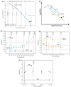 |
Fig. 1. Example of a type II spectrum that shows a single range of close-to-IK scaling across the full IR for PSP/FIELDS measurements of the full trace of power spectral tensor, taken over a 12 h interval at 0.5 AU with local plasma β = 0.53. (a): Log-log plot of PSD versus frequency. The plotted points result from a Haar wavelet analysis of the dataset; they are marked as blue circles in the IR identified here and as grey asterisks outside it. (b): Procedural diagram for the two adjacent scatter plots used to identify the IR and its single best-fit gradient (see text). Breakpoints at the upper and lower end of the IR are identified by locating scale-by-scale increases in the 95% confidence interval (CI) of the exponent using the method outlined in Sect. 2.2, as shown in panels c, d, and e. (c): Spectral exponent and its CI, on the blue pathway labelled (i) beginning at Start and ending at Q in the procedural diagram above. (d): Same as panel c, but for the yellow pathway labelled (ii) beginning at Q and descending to the first blue circle, labelled P. (e): CI for pathway (iv), showing that the ‘1/f’ range continues to the 16th point, labelled T. |
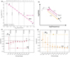 |
Fig. 2. Example of a type IV spectrum that shows a single range of scaling close to Kolmogorov across the full IR for PSP/FIELDS measurements of the full trace of power spectral tensor, taken over a 3 h interval at 0.70 AU with local plasma β = 3.71. (a): Log-log plot of PSD versus frequency. Plotted points result from a Haar wavelet analysis of the dataset; they are marked as pink circles in the IR identified here and as a grey asterisk outside it. (b): Procedural diagram for the two adjacent scatter plots used to identify the IR and its single best-fit gradient. Breakpoints at the upper and lower end of the IR were identified by locating sudden increases in the CI of the exponent using the method outlined in Sect. 2.2, as shown in panels c and d. (c): Spectral exponent and its CI on the pink pathway labelled (i) beginning at Start and ending at Q in the procedural diagram above. (d): Same as panel c, but for the yellow pathway labelled (ii) beginning at Q and descending to the first pink circle, labelled P. |
We considered a finite range power-law region of the PSD, Uk, m, comprised of wavelet power estimates Wk, Wk + 1, …, Wm estimated at each wavelet scale j = k, k + 1, …, m, at central frequencies fj. Higher values of j correspond to lower frequencies. Each estimate of the power spectral exponent based on Uk, m will have an uncertainty ϵk, m. We obtained both the value of the power spectral exponent and its uncertainty from a linear least squares fit to the sequence of Wj, fj in the Uk, m region.
Once a power-law range was identified in the PSD, a linear least squares fit was performed in log-log space to obtain the spectral exponent and the fit uncertainty; here we quote 95% confidence bounds on the fitted power spectral exponent throughout. The following procedure was used to estimate the frequencies of the upper and lower bounds of the power-law range of scaling at breakpoint frequencies fP and fQ.
-
Estimate the power spectral exponent from Uk, k + l, where the wavelet temporal scale, k, lies within the power-law region of the PSD at the central frequency, fk.
-
Successively increase the frequency range, in the direction of decreasing frequency, by considering l = 1, 2, 3, …, and at each value of l estimate the power spectral exponent.
-
Test if ϵk, k + l > ϵk, k + l + 1; if true, increment l.
-
If ϵk, k + l < ϵk, k + l + 1, then the low-frequency breakpoint Q = k + l has been reached.
-
Now estimate the power spectral exponent from UQ − l, Q.
-
Successively increase the frequency range, in the direction of increasing frequency, by considering l = 1, 2, 3, …, and at each value of l estimate the power spectral exponent.
-
Test if ϵQ − l, Q > ϵQ − l − 1, Q; if true, increment l.
-
If ϵQ − l, Q < ϵQ − l − 1, Q, then the high-frequency breakpoint k = Q − l = P has been reached.
In this study, we only considered intervals of PSP data where there is a clearly identifiable transition between the IR and the‘1/f’ range. However, we find that they do not all correspond to the simple case outlined in the preceding paragraph. In particular, our procedure has identified cases where the low-frequency breakpoint, Q, is clearly at a higher frequency than the transition between the IR and ‘1/f’ range. Examples are shown in Figs. 3 and 4. In these cases, we applied the above procedure to search for the IR–‘1/f’ transition as follows:
-
Estimate the power spectral exponent from UQ, Q + l, where wavelet temporal scale k = Q has been determined as above.
-
Successively increase the frequency range by considering l = 1, 2, 3, …, and at each value of l estimate the power spectral exponent.
-
Test if ϵQ, Q + l > ϵQ, Q + l + 1; if true, increment l.
-
If ϵQ, Q + l < ϵQ, Q + l + 1, then the low-frequency breakpoint m = Q + l = R has been reached.
 |
Fig. 3. Example of a type III spectrum that shows two ranges of scaling within the IR: close to Kolmogorov scaling at higher frequencies (pink circles in the top panel; the asterisks lie outside this range) and a shallower range (at lower frequencies; i.e. the green circles in panel a). The interval is for PSP/FIELDS measurements of the full trace of power spectral tensor taken over a 5 h interval at 0.61 AU with local plasma β = 1.02. (a): Log-log plot of PSD versus frequency. The plotted points result from a Haar wavelet analysis of the dataset. (b): Procedural diagram for panels c to e used to identify the breakpoints between the three scaling ranges, together with their best-fit gradients. Breakpoints at the point labelled Q (between gradients –1.73 and –1.39) and at the point labelled R (between IR gradient –1.39 and ‘1/f’ range; the latter terminates at the point labelled T) were identified from the CI of the exponent using the method outlined in Sect. 2.2, the exponents and CI are displayed in panels c to e. (c): Minimum exponent CI located at the point labelled Q for pathway (i) extending from point 3 upwards (pink). The continuation of the pathway (i) beyond point 7 suggests a second breakpoint at point 13, where the CI suddenly increases. (d): Pathway (ii) descending from point 7 (yellow). It has the minimum CI when it encompasses points down to point 2. (e): Exponent and CI for pathway (iii), in green. This confirms the breakpoint at the point labelled R. |
This determines the wavelet scale, R, and frequency, fR, as an upper limit on the transition between the IR and the ‘1/f’ range.
3. Results
3.1. Example spectra
We applied the above procedure to PSP intervals, selected across a wide range of radial distances from the Sun and hence across a correspondingly wide range of local plasma β. We find that the spectra can be classified into four types according to their overall morphology. They are: Type I, which can be fitted by two ranges of scaling within the IR; the inner, high-frequency range has an exponent close to Iroshnikov-Kraichnan (IK), whereas the low-frequency range is shallower. Type II can be fitted by a single IR of scaling with exponents between the IK and Kolmogorov values. Type III can be fitted by two ranges of scaling within the IR; the inner, high-frequency range has an exponent close to Kolmogorov, whereas the low-frequency range is shallower. Finally, type IV can be fitted by a single IR of scaling with exponents close to Kolmogorov. This classification is ordered by distance from the Sun. In all cases, a clear transition to the ‘1/f’ range of scaling is identified in the spectra.
We have first plotted the PSD for four intervals, representing each of these types, at different heliospheric distances to illustrate the procedure for identifying power-law ranges in the PSD and estimating the power spectral exponents.
The top panels of Figs. 1–4 show the DWT estimates of the PSD for the trace of the power spectral tensor. Different colours and symbols are used to indicate the distinct power-law ranges where they can be identified using the method described above. Where a clear ‘1/f’ range (that is, fα, where the index α is some negative number) can be identified, it is indicated by black triangles. The IR is indicated by circles with pink indicating a scaling exponent close to Kolmogorov, α = −5/3, and blue a scaling exponent close to IK, α = −3/2.
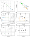 |
Fig. 4. Example of a type I spectrum that shows two ranges of scaling within the IR with an exponent close to IK at higher frequencies (blue circles in the top panel) and a shallower range at lower frequencies (green circles in panel a). There is a transition ‘1/f’ scaling at the lowest frequencies (black triangles in panel a). The interval is for PSP/FIELDS measurements of the full trace of the power spectral tensor, taken over a 48 h interval at 0.17 AU with local plasma β = 0.34. (a): Log-log plot of PSD versus frequency. The plotted points result from a Haar wavelet analysis of the dataset. (b): Procedural diagram for the four plots used to identify the breakpoints between three scaling ranges and their best-fit gradients. Breakpoints at the point labelled Q (between gradients –1.52 and –1.25) and the point labelled R (between IR gradient –1.25 and ‘1/f’; the latter terminates at the point labelled T) were identified from the CI of the exponent using the method outlined in Sect. 2.2 and are displayed in panels c to f. (c): Minimum exponent CI located at the point labelled Q for pathway (i) extending from point 3 upwards (blue). The continuation of the pathway (i) beyond point 8 suggests a second breakpoint at point 12, where the CI suddenly increases. (d): Pathway (ii) descending from point 8 (yellow). It has a minimum CI when it encompasses points down to the third scale. (e): Exponent and CI for pathway (iii), in green. This confirms the breakpoint at the point labelled R. (f): Exponent and CI for pathway (iv), showing that the ‘1/f’ range continues to the point labelled T. |
The kinetic range, and in many cases the ‘1/f’ range, is not fully resolved as distinct power-law ranges in these observations; nevertheless, they are clearly identified as being outside of the IR via the breakpoint finding procedure. These points are indicated by grey asterisks on the plots.
The DWT temporal scales, j, converted to frequencies f = f02−j Hz, where f0 = 1/(2dt) Hz (dt is the cadence of the observations), are indicated at the top of these panels. The wavelet temporal scales at which breakpoints were identified using the above iterative procedures are indicated on the spectra. The iterative procedure is summarised for each of these spectra in the schematic (centre panel). Figure 1 shows the IR power-law spectral exponent for a 12 h interval of turbulent solar wind at a heliospheric distance 0.5 AU and for β = 0.53.
In Fig. 1 the procedure is shown beginning at the wavelet temporal scale labelled Start and is first applied along the path labelled (i) from higher to lower frequencies to determine the low-frequency end of the IR (Q), which is a transition to the ‘1/f’ range. It is then applied along the path labelled (ii) from lower frequencies to higher to determine the high-frequency end of the IR (P), which is a transition to the kinetic range. The fitted power-law exponent and its uncertainty for each iteration are plotted in the last two panels for each sequence of iterations, (i) and (ii). As more wavelet scales are successively included in the fitting range, the uncertainty decreases. The uncertainty remains small, and the value of the fitted exponent remains constant until the fitting range extends beyond the power-law range of the spectrum. For comparison, horizontal dashed lines indicate power-law scaling exponents of α = −3/2 and α = −5/3, and we can see that for this interval of turbulent solar wind, the scaling is clearly identified as between IK α = −3/2 and Kolmogorov α = −5/3. In this case, the ‘1/f’ range is discerned at lower frequencies and is clearly distinct from the IR.
Figure 2 shows the spectrum obtained for a 3 h interval of turbulent solar wind at a heliospheric distance 0.7 AU and for β = 3.71. In this case, our procedure identifies a single scaling region, but the scaling exponent now approximates Kolmogorov α = −5/3 scaling. In this case, the interval is not long enough to fully resolve a clear power-law ‘1/f’ range.
Our method identifies all breakpoints in the wavelet spectra, without assuming the existence of specific power-law ranges. We have found cases where the spectra are well described by an IR composed of two power-law regions with distinct scaling exponents. Two examples are presented in Figs. 3 and 4, which correspond to a 5 h interval with local plasma β = 1.02 at 0.61 AU and a 48 h interval with local plasma β = 0.34 at 0.17 AU, respectively.
In Fig. 3 the IR is best fitted by a power-law range from wavelet scale 2 to scale 7 (temporal scales from 0.9 s to 28.0 s, with corresponding frequencies spanning from 0.04 Hz to 1.11 Hz), where the scaling is close to Kolmogorov, the fitted line is of exponent –1.73 [–1.75, –1.71], and there is a second power law from wavelet scale 7 to scale 13 (temporal scales from 28.0 s to 30.0 min, with corresponding frequencies spanning from 5.56 × 10⁻⁴ Hz to 0.04 Hz) with exponent –1.39 [–1.47, –1.31]. This identifies a break in scaling at about 30 s within the IR, with the full IR occupying the range from wavelet scale 2 to scale 13, that is, from approximately 0.9 s to about 30.0 min, with corresponding frequencies spanning from 5.56 × 10⁻⁴ Hz to 1.11 Hz. To illustrate this, we extended the fitted line from wavelet scales from scale 7 to scale 13 (temporal scales from 28.0 s to 30.0 min, with corresponding frequencies spanning from 5.56 × 10⁻⁴ Hz to 0.04 Hz). It is clear that for timescales longer than scale 8, or about 1 min, the observed spectrum progressively deviates from the fitted line. A second example is provided in Fig. 4, where wavelet scale 3 to scale 8 (temporal scales from 1.8 s to 1 min, with corresponding frequencies spanning from 1.67 × 10⁻² Hz to 0.56 Hz) follow IK scaling within narrow error bars (gradient = –1.52 [–1.53, –1.52]), whereas wavelet scale 8 to scale 12 (temporal scales from 1 min to 14.9 min, with corresponding frequencies spanning from 1.12 × 10⁻³ Hz to 1.67 × 10⁻² Hz) are fitted by a power-law spectrum with a lower exponent, –1.25[–1.42, –1.09], with uncertainties that exclude the IK value of α = −3/2. This is again illustrated by extending the fitted line for scale 8 to scale 12 (temporal scales from 1 min to 14.9 min, with corresponding frequencies spanning from 1.12 × 10⁻³ Hz to 1.67 × 10⁻² Hz). In this case, the ‘1/f’ range is clearly identified at lower frequencies and is distinct from the lower-frequency part of the IR. For comparison, we took the spectra plotted in Figs. 3 and 4 and instead fitted a single power law to the range between wavelet scales R and P with temporal scales from 0.9 s (1.11 Hz) to 30.0 min (5.56 × 10⁻⁴ Hz) and from 1.8 s (0.56 Hz) to 14.9 min (1.12 × 10⁻³ Hz), respectively. This is shown in Figs. 5 and 6, respectively. The resultant exponents have an uncertainty that is reasonable (about 4%) but is larger than that obtained by fitting two spectral ranges (for the high-frequency ranges of Figs. 3 and 4, it is about 1%). Thus, whilst we do not suggest these results provide an unambiguous discrimination between a single and dual scaling IR, it raises the question of how often, and under what conditions, dual scaling can occur and be detected in the IR.
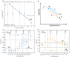 |
Fig. 5. Fit of a single gradient to the full IR of the data in Fig. 3. This fitting approach results in IK scaling within an acceptable uncertainty (shown in blue). The wavelet points in the IR are denoted by blue circles. (a): Log-log plot of PSD versus frequency. The plotted points result from a Haar wavelet analysis of the dataset. (b): Procedural diagram for panels c and d, used to identify the breakpoints between the three scaling ranges, together with their best-fit gradients. Breakpoints at the point labelled R (between IR gradient –1.55 and ‘1/f’ range; the latter terminates at the point labelled T) were identified from the CI of the exponent using the method outlined in Sect. 2.2 and are displayed in panels c and d. (c): Spectral exponent and its CI on the blue pathway labelled (i) beginning at Start and ending at R in the procedural diagram above. (d): Pathway (ii) descending from point 13 (yellow). It has the minimum CI when it encompasses points down to point 2. |
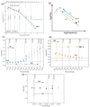 |
Fig. 6. Fit of a single gradient to the full IR of the data in Fig. 4 (counterpart to Figs. 5 and 3). This fitting approach results in IK scaling with an acceptable uncertainty (shown in blue). The wavelet points in the IR are denoted by blue circles, while black triangles represent those in the ‘1/f’ range. |
3.2. Spectral exponent survey
Both the range of scaling and the scaling exponent of the IR (Chen et al. 2020; Alberti et al. 2020) are known to evolve with distance from the Sun. To examine how the IR evolves with distance from the Sun and with plasma β, we performed a scan of the first four PSP orbits. In Table 1 we list the results for all intervals that satisfy our criteria for homogeneous turbulence and have clearly identified crossovers to both a kinetic range and a ‘1/f’ range of scaling. The range of values of plasma β, and distance from the Sun are plotted in Fig. 7.
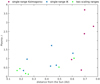 |
Fig. 7. Distribution of individual intervals, categorised into three distinct types: single-range Kolmogorov (pink circles); single-range IK (blue triangles); and dual-scaling range (green hexagrams). The x-axis plots the distance from the Sun, while the y-axis plots the local plasma β. |
IR magnetic field trace PSD power law exponent a with 95% CL bounds [b c] of each event listed in order of increasing distance from the Sun d (AU) with plasma β and classification type (see text).
A significant proportion of these intervals are found to have a breakpoint within the IR, and in these cases, the temporal scales of the dual scaling ranges found using the above procedure are listed. In all these cases, we quantified the percentage uncertainty on the power-law scaling exponents and, in the cases where our procedure finds a dual-range IR, we obtained the exponents and uncertainties for both a single range of scaling IR (a single power law) and a dual-range IR (two power laws). Looking across these, it is clear that in some cases the single power-law fit and dual power-law fit give comparable uncertainties. In other cases, however, the dual-power-law fit gives a lower uncertainty in the high-frequency scaling range.
Figures 8 and 9 show how the IR power-law range scaling exponents are ordered by distance from the Sun and plasma β. The upper and middle panels of Figs. 8 and 9 show the obtained spectral exponents with 95% confidence intervals as a function of distance from the Sun; the middle panels present a zoomed-in view of the upper panels. In cases where a fully resolved ‘1/f’ range is found, its exponent is plotted in the upper panel (green symbols). The ‘1/f’ range scaling exponent shows significant variation between intervals; however, it is distinct from that found for the IR. The intervals where a distinct ‘1/f’ range is clearly resolved are at locations spanning 0.17 AU to 0.70 AU; however, they all correspond to local plasma β ≤ 2.5. Intervals, where an unbroken IR range of scaling with a single exponent is determined via the above procedure are indicated with red symbols in the figures. The scaling exponents found for these cases are closer to IK scaling for distances ≤0.5 AU but are closer to Kolmogorov scaling beyond 0.6 AU. Single unbroken IR scaling with exponents spanning Kolmogorov and IK values are found at all values of plasma β. In cases where the exponent is closer to Kolmogorov, the ideal α = −5/3 value often lies well outside the uncertainties. These intervals that show a single unbroken IR of scaling are thus consistent with the previous studies. Previous spectral estimates based on DFT identified a drift towards approximately Kolmogorov scaling with increasing distance from the Sun beyond 1 AU (Roberts 2010) and, specifically with PSP, a drift from approximately Kolmogorov scaling at around 1 AU to approximately IK scaling closer to the Sun (Chen et al. 2020). However, these previous studies identified a gradual change, whereas here we see a transition between Kolmogorov and IK at a distance between 0.5 AU and 0.6 AU. The intervals studied here sample a broad range of values of plasma β, as shown in Fig. 9. The lower panels of Figs. 8 and 9 show the transitions to the ‘1/f’ and kinetic ranges. The above methodology for detecting breakpoints identifies the first wavelet scale outside of the IR so that the frequency of the transition to ‘1/f’, and the kinetic range, are respectively the upper and lower bounds in frequency (the transition to ‘1/f’ can occur at a lower frequency, and the transition to the KR can occur a higher frequency). Irrespective of position and local plasma β, the high-frequency KR is close to 1 Hz, and the low-frequency ‘1/f’ transition point corresponds to a period of a few minutes to an hour. Intervals where our procedure identifies two distinct scaling ranges within the IR are found at a range of distances from the Sun, but all occur for plasma β ≲ 1. In contrast, single unbroken IR scaling is found at β > 0.5 (see Fig. 9).
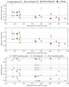 |
Fig. 8. Fitted power-law range PSD exponent plotted versus distance from the Sun (upper, mid panels) and of frequencies at which spectral breakpoints are found (lower panel), for the PSD trace for intervals in Figs. 1–4 and Table 1. Upper panel: fitted spectral exponents plotted versus distance from the Sun, spanning 0.15 AU to 0.8 AU, for sub-ranges of the wavelet-derived spectrum that we have identified as: ‘1/f’ (grey squares); type I spectra (green); type II spectra (blue); type III spectra (orange); type IV spectra (pink); single IR (diamonds); and IR containing a breakpoint, with exponents for the upper (triangles) and lower frequency ranges (circles) displayed separately. The horizontal dot-dash lines mark the IK (upper) and Kolmogorov (lower) values. Middle panel: Zoon in of the top panel with ‘1/f’ exponents excluded and covering a narrower range of exponent values, between –1 and –2. Lower panel: Frequency limits of the IR identified as transitions to ‘1/f’scaling (yellow squares) and to the KR (blue diamonds), together with the frequency location of the breakpoint within the IR (black hexagrams), if found. Horizontal dot-dash lines indicate frequencies that correspond to periods between 1 s and 1 h. |
The lower panels of Figs. 8 and 9 show where the breakpoint within the IR occurs in frequency, relative to the crossover to the ‘1/f’ and kinetic ranges. Importantly, these breakpoints within the IR are found with periods in the range of approximately 30 s to a few minutes; they are well separated in frequency and wavelet scale from the termination of the IR at the transitions to ‘1/f’ and kinetic range. In most of these cases we have identified a clear termination of IR scaling and transition to ‘1/f’ regions of the spectrum and in some cases a clear power-law ‘1/f’ range. There are several possibilities for interpreting these IR spectra: (i) as two power-law ranges with different exponents, (ii) as a single power-law range, and (iii) as a monotonic deviation from the power law, as in the case of generalised similarity (Frisch 1995), which has been found in solar wind turbulence at the early stages of its evolution (Chapman & Nicol 2009). Interpretation (iii) may explain some of our results, as in Fig. 8 we see that dual ranges of scaling within the IR are found within 0.3 AU, consistent with a less well-developed turbulent cascade. Interpretations (i) and (ii) for some intervals give essentially the same uncertainties, so Occam’s razor favours interpretation (ii), namely a single power-law IR. However, as detailed in Table 1, there are several cases where fitting two power-law ranges significantly reduces the uncertainty in the exponent at higher frequencies, motivating further study. We emphasise the need for comparison, supported by uncertainty estimates, between the two distinct hypotheses of a single IR and two IR ranges of scaling. Previous results, for example that of Telloni (2022), have identified candidate dual-scaling IR spectra; however, this example was estimated via DFT and did not include uncertainty estimates on the spectral exponents.
Figures 8 and 9, show a pattern in the distinct scaling behaviour suggesting a classification of the results into four types. Type I spectra are found within a radial distance of 0.3 AU from the Sun. These spectra exhibit two distinct scaling ranges. The inner range, characterised by high frequencies, has scaling exponents consistent with the IR IK theory within uncertainties. On the other hand, the outer range, at lower frequencies, has shallower scaling exponents ranging from –1.28 to –1.23. Type II spectra occur between 0.4 and 0.5 AU. They have scaling exponents closer to, yet steeper than, the expected IK value of α = −3/2. However, these exponents do not align precisely with the IK value within estimated uncertainties. At two specific distances, namely 0.26 AU and 0.61 AU, type III spectra were observed. They exhibit two distinct scaling ranges. The outer range, corresponding to lower frequencies, has an exponent of approximately –1.4. The high-frequency range, however, has scaling behaviour close to the Kolmogorov theory α = −5/3. Notably, these spectra are found at the transitions between type I and type II as well as between type II and type IV spectra. Beyond 0.5 AU from the Sun, type IV spectra were found. They display scaling exponents close to, but mostly steeper than, Kolmogorov. Our study also determined a lower bound on the frequency of the transition to the kinetic range of approximately 1 Hz. Importantly, this lower bound does not show a dependence on the plasma β, or the distance from the Sun. Furthermore, an upper bound on the frequency of the transition to the ‘1/f’ range was established for all intervals considered in this study. A tendency was found for type I spectra to be associated with β < 1. Conversely, type IV spectra were found across all values of β. However, we emphasise that none of the intervals within 0.4 AU included high β values.
4. Conclusions
Whilst it is well established that there is an IR of MHD turbulence in the solar wind, there has been considerable discussion regarding the value of the exponent of the observed power-law PSD, which varies with distance from the Sun (Chen et al. 2020; Roberts 2010). The value of the exponent is a key prediction in turbulence theories (Kraichnan 1965; Iroshnikov 1964; Kolmogorov 1941) as it is not universal (Chapman & Hnat 2007).
We applied a systematic method to quantify the spectral breaks and scaling exponents from extended intervals of turbulence observed by PSP at different distances from the Sun and over a range of plasma β. Wavelets provide a natural tool for estimating the exponents of power-law spectra as they provide a linear sampling of the log-frequency domain. We used undecimated DWT Haar wavelet estimates of the PSD for multiple, long-duration intervals of uniform solar wind turbulence, sampled by PSP/FIELDS and selected to exclude coherent structures, such as pressure pulses and current sheets, in which the primary proton population velocity varies by less than 20% of its mean value. Intervals were only included in the study where there is a clear identification of the approximately ‘1/f’ range at low frequencies, an MHD IR of turbulence, and a kinetic range below the ion gyrofrequency. We can classify the spectra into four categories as follows:
-
Type I: Within 0.3 AU of the Sun, the IR exhibits two distinct ranges of scaling. The inner, high-frequency range has an exponent consistent with that of IK within the uncertainties. The outer, low-frequency range is shallower, with exponents in the range from –1.28 to –1.23.
-
Type II: Between 0.3 and 0.5 AU, the IR exponents are closer to, but steeper than, that of IK and do not coincide with the value α = −3/2 within uncertainties.
-
Type III: At 0.26 AU and at 0.61 AU, the IR has two distinct ranges of scaling. The outer, low-frequency range has an exponent ∼ − 1.4 and the high-frequency range has an exponent close to that of Kolmogorov. These spectra are found at the transitions between type I and type II spectra and between type II and type IV spectra.
-
Type IV: At distances beyond 0.5 AU from the Sun, the exponents are close to, but mostly steeper than, Kolmogorov: uncertainties inherent in the observed exponents exclude the value α = −5/3.
-
We determine a lower bound on the frequency of the transition to the dissipation range at ∼1 Hz, which is not sensitive to plasma, β, or distance from the Sun.
-
We determine an upper bound on the frequency of the transition to the ‘1/f’ range in all intervals considered in this study.
-
There is a tendency for type I spectra to be found at β < 1, and type IV spectra are found at all β; however, none of our intervals include high β within 0.4 AU.
Since the PSD-estimated scaling exponents are a central prediction of turbulence theories, these results provide new insights into the evolution of turbulence in the solar wind. We have obtained estimates of the scaling exponents and scale breaks of the power spectra of MHD turbulence at sufficient precision to discriminate between Kolmogorov and IK turbulence, both within each spectrum and across multiple samples. Whilst we confirm the previously identified evolution from Kolmogorov-like scaling to IK-like scaling with decreasing distance from the Sun, the Kolmogorov-like values, which we find almost exclusively beyond 0.5 AU, are not in fact consistent with a α = −5/3 spectral exponent within the fit uncertainties. Thus, whilst the average over many spectral estimates at larger distances from the Sun may approach an exponent of α ≈ −5/3, as found previously (Chen et al. 2020) the individual spectral exponents are not consistent with this exponent. This is distinct from the behaviour within 0.5 AU, where the exponents of each individual spectrum coincide with α = −3/2 IK scaling rather than in an average sense.
This discrepancy in the observed and theoretically expected exponents may arise from the choice of magnetic field fluctuation coordinate system and from the anisotropic nature of these fluctuations, which we do not address here. Coordinate systems that align with a globally averaged background field (Matthaeus et al. 2012; Horbury et al. 2012; TenBarge et al. 2012; Zhao et al. 2022) or with the local scale-by-scale field (Kiyani et al. 2013; Horbury et al. 2008), have both been proposed, as has binned the fluctuations with reference to the local field direction (Osman et al. 2014). Establishing whether working in these coordinate systems can systematically resolve the above discrepancy will be the topic of future work. This discrepancy raises the question as to what precision we need the observed power-law exponents to agree with theoretical predictions in order to confirm a given turbulence phenomenology?
A transition between Kolmogorov and IK scaling within MHD IR scales at approximately 0.5 AU may be a distinct phenomenology of the solar wind at this heliospheric distance. There is some evidence that the effects of coronal events, such as coronal mass ejections or coronal hole jets, are incorporated into turbulent solar wind at scales greater than 0.3 AU (Owens et al. 2017; Horbury et al. 2018). Alternatively, the transition may reflect, for example, the changes in the imbalance in IK turbulence (Galtier et al. 2001) or a varying level of the dynamic alignment between the magnetic field and the velocity fluctuations (Meyrand et al. 2016) at these scales.
We have found examples where the IR is well described by two power-law sub-ranges with different scaling exponents. These breakpoints within the IR are found with periods in the range 30 s to 10 min. The breakpoints within the IR are well separated in frequency and wavelet scale from the termination of the IR at the transitions to the ‘1/f’ range and KR. Interpretations of these IR spectra include: two power-law ranges with different exponents; a single power-law range with generally increased uncertainty, particularly at higher frequencies; or a monotonic deviation from a power law. The suggestion of a two-power-law IR is currently tentative, and additional research is needed to clarify or resolve this matter. The selection of an appropriate magnetic coordinate system in particular requires further investigation. Nevertheless, these results motivate further study and emphasise the importance of precise estimations of power-law exponents and their uncertainties when attempting to connect these observations with theoretical predictions. A coexistence of IK and Kolmogorov turbulence within the scales we traditionally refer to as MHD IR is important in models of solar wind heating (see for example Chandran et al. 2011).
Acknowledgments
We acknowledge the NASA Parker Solar Probe Mission, and the FIELDS team led by S. D. Bale, and the SWEAP team led by R. Kasper for the use of data. The FIELDS experiment on the Parker Solar Probe spacecraft was designed and developed under NASA contract NNN06AA01C. S.C.C. and B.H. acknowledge AFOSR grant FA8655-22-1-7056 and STFC grant ST/T000252/1. S.C.C. acknowledges support from ISSI via the J. Geiss fellowship.
References
- Alberti, T., Laurenza, M., Consolini, G., et al. 2020, ApJ., 902, 84 [NASA ADS] [CrossRef] [Google Scholar]
- Bale, S., Goetz, K., Harvey, P., et al. 2016, Space Sci. Rev., 204, 49 [Google Scholar]
- Barenblatt, G. 1996, Scaling, Self-similarity, and Intermediate Asymptotics (Cambridge University Press) [CrossRef] [Google Scholar]
- Bruno, R., & Carbone, V. 2013, Liv. Rev. Sol. Phys., 2, 10 [Google Scholar]
- Bruno, R., Carbone, V., Primavera, L., et al. 2004, Ann. Geophys., 22, 3751 [Google Scholar]
- Buckingham, E. 1914, Phys. Rev., 4, 345 [CrossRef] [Google Scholar]
- Chandran, B. D., Dennis, T. J., Quataert, E., et al. 2011, ApJ, 743, 197 [NASA ADS] [CrossRef] [Google Scholar]
- Chapman, S., & Hnat, B. 2007, Geophys. Res. Lett., 34, L17103 [NASA ADS] [CrossRef] [Google Scholar]
- Chapman, S., & Nicol, R. 2009, Phys. Rev. Lett., 103, 241101 [NASA ADS] [CrossRef] [Google Scholar]
- Chapman, S., Hnat, B., Rowlands, G., et al. 2005, Nonlinear Proc. Geophys., 12, 767 [NASA ADS] [CrossRef] [Google Scholar]
- Chen, C. H. K. 2016, J. Plasma Phys., 82, 6 [NASA ADS] [CrossRef] [Google Scholar]
- Chen, C. H. K., Leung, L., Boldyrev, S., et al. 2014, Geophys. Res. Lett., 41, 8081 [NASA ADS] [CrossRef] [Google Scholar]
- Chen, C., Bale, S., Bonnell, J., et al. 2020, ApJS, 246, 53 [Google Scholar]
- Davis, N., Chandran, B., Bowen, T., et al. 2023, ApJ, 950, 154 [NASA ADS] [CrossRef] [Google Scholar]
- Feynman, J., & Ruzmaikin, A. 1994, J. Geophys. Res. Space Phys., 99, 17645 [NASA ADS] [CrossRef] [Google Scholar]
- Fox, N., Velli, M., Bale, S., et al. 2016, Space Sci. Rev., 204, 7 [Google Scholar]
- Frisch, U. 1995, Astrophysical Letters And Communications (Cambridge University Press) [Google Scholar]
- Galtier, S., Nazarenko, S. V., Newell, A. C., et al. 2001, ApJ, 564, L49 [Google Scholar]
- Gogoberidze, G., & Voitenko, Y. M. 2016, Ap&SS, 361, 1 [NASA ADS] [CrossRef] [Google Scholar]
- Goldreich, P., & Sridhar, S. 1995, ApJ, 438, 763 [Google Scholar]
- Hnat, B., Chapman, S., Gogoberidze, G., et al. 2011, Phys. Rev. E., 84, 065401 [NASA ADS] [CrossRef] [Google Scholar]
- Horbury, T. S., & Balogh, A. 1997, Nonlinear Proc. Geophys., 4, 185 [NASA ADS] [CrossRef] [Google Scholar]
- Horbury, T., Forman, M., & Oughton, S. 2008, Phys. Rev. Lett., 101, e175005 [NASA ADS] [CrossRef] [Google Scholar]
- Horbury, T. S., Wicks, R. T., & Chen, C. H. K. 2012, Space Sci. Rev., 172, 325 [Google Scholar]
- Horbury, T. S., Matteini, L., & Stansby, D. 2018, MNRAS, 478, 1980 [Google Scholar]
- Iroshnikov, P. 1964, Sov. Astron., 7, 566 [Google Scholar]
- Kasper, J., Abiad, R., Austin, G., et al. 2016, Space Sci. Rev., 204, 131 [NASA ADS] [CrossRef] [Google Scholar]
- Kiyani, K., Chapman, S., Sahraoui, F., et al. 2013, ApJ, 763, 10 [NASA ADS] [CrossRef] [Google Scholar]
- Kiyani, K. H., Osman, K. T., & Chapman, S. 2015, Phil. Trans. R. Soc. A, 373, 20140155 [CrossRef] [Google Scholar]
- Kolmogorov, A. 1941, Akademiia Nauk SSSR Doklady, 30, 301 [Google Scholar]
- Kraichnan, R. 1965, Phys. Fluids, 8, 1385 [NASA ADS] [CrossRef] [Google Scholar]
- Longair, M. 2003, High Energy Astrophysics (Cambridge University Press) [Google Scholar]
- Matthaeus, W. H., Breech, B., Dmitruk, P., et al. 2007, ApJ, 657, L121 [NASA ADS] [CrossRef] [Google Scholar]
- Matthaeus, W. H., Servidio, S., Dmitruk, P., et al. 2012, ApJ, 750, 103 [NASA ADS] [CrossRef] [Google Scholar]
- Meyrand, R., Galtier, S., & Kiyani, K. H. 2016, Phys. Rev. Lett., 116, 105002 [NASA ADS] [CrossRef] [Google Scholar]
- Nicol, R. M., Chapman, S. C., & Dendy, R. O. 2009, ApJ, 703, 2138 [NASA ADS] [CrossRef] [Google Scholar]
- Osman, K., Kiyani, K., Chapman, S., et al. 2014, ApJ, 783, L27 [CrossRef] [Google Scholar]
- Owens, M. J., Lockwood, M., & Barnard, L. A. 2017, Sci. Rep., 7, 1 [CrossRef] [Google Scholar]
- Politano, H., & Pouquet, A. 1995, Phys. Rev. E, 52, 636 [NASA ADS] [CrossRef] [Google Scholar]
- Roberts, A. 2010, J. Geophys. Res., 115, A12101 [NASA ADS] [Google Scholar]
- Salem, C., Mangeney, A., Bale, S. D., et al. 2009, ApJ, 702, 537 [NASA ADS] [CrossRef] [Google Scholar]
- Sioulas, N., Huang, Z., Shi, C., et al. 2023, ApJ, 943, L8 [CrossRef] [Google Scholar]
- Sorriso-Valvo, L., Marino, R., Lijoi, L., et al. 2015, ApJ, 807, 86 [NASA ADS] [CrossRef] [Google Scholar]
- Telloni, D. 2022, Front. Astron. Space Sci., 9, 856188 [NASA ADS] [CrossRef] [Google Scholar]
- TenBarge, J. M., Podesta, J. J., Klein, K. G., et al. 2012, ApJ, 753, 107 [NASA ADS] [CrossRef] [Google Scholar]
- Tu, C., & Marsch, E. 1995, Space Sci. Rev., 73, 1 [NASA ADS] [CrossRef] [Google Scholar]
- Verma, M. 1999, Phys. Plasmas, 6, 1455 [NASA ADS] [CrossRef] [Google Scholar]
- Verscharen, D., & Klein, K. 2019, Liv. Rev. Sol. Phys., 16, 5 [NASA ADS] [CrossRef] [Google Scholar]
- Wang, X., Chapman, S., Dendy, R., et al. 2022, 48th EPS Conference on Plasma Physics https://indico.fusenet.eu/event/28/contributions/359/ [Google Scholar]
- Welch, P. D. 1967, IEEE Trans. Audio Electroacoust., 15, 70 [CrossRef] [Google Scholar]
- Wicks, R., Horbury, T., Chen, C., et al. 2010, MNRAS, 407, L31 [NASA ADS] [CrossRef] [Google Scholar]
- Wicks, R., Forman, M., Horbury, T., et al. 2012, ApJ, 746, 103 [NASA ADS] [CrossRef] [Google Scholar]
- Zhao, L., Zank, G., Adhikari, L., et al. 2022, ApJ, 924, L5 [NASA ADS] [CrossRef] [Google Scholar]
- Zhou, Y., Matthaeus, W., & Dmitruk, P. 2004, Rev. Mod. Phys., 76, 1015 [NASA ADS] [CrossRef] [Google Scholar]
All Tables
IR magnetic field trace PSD power law exponent a with 95% CL bounds [b c] of each event listed in order of increasing distance from the Sun d (AU) with plasma β and classification type (see text).
All Figures
|
Fig. 1. Example of a type II spectrum that shows a single range of close-to-IK scaling across the full IR for PSP/FIELDS measurements of the full trace of power spectral tensor, taken over a 12 h interval at 0.5 AU with local plasma β = 0.53. (a): Log-log plot of PSD versus frequency. The plotted points result from a Haar wavelet analysis of the dataset; they are marked as blue circles in the IR identified here and as grey asterisks outside it. (b): Procedural diagram for the two adjacent scatter plots used to identify the IR and its single best-fit gradient (see text). Breakpoints at the upper and lower end of the IR are identified by locating scale-by-scale increases in the 95% confidence interval (CI) of the exponent using the method outlined in Sect. 2.2, as shown in panels c, d, and e. (c): Spectral exponent and its CI, on the blue pathway labelled (i) beginning at Start and ending at Q in the procedural diagram above. (d): Same as panel c, but for the yellow pathway labelled (ii) beginning at Q and descending to the first blue circle, labelled P. (e): CI for pathway (iv), showing that the ‘1/f’ range continues to the 16th point, labelled T. |
| In the text | |
|
Fig. 2. Example of a type IV spectrum that shows a single range of scaling close to Kolmogorov across the full IR for PSP/FIELDS measurements of the full trace of power spectral tensor, taken over a 3 h interval at 0.70 AU with local plasma β = 3.71. (a): Log-log plot of PSD versus frequency. Plotted points result from a Haar wavelet analysis of the dataset; they are marked as pink circles in the IR identified here and as a grey asterisk outside it. (b): Procedural diagram for the two adjacent scatter plots used to identify the IR and its single best-fit gradient. Breakpoints at the upper and lower end of the IR were identified by locating sudden increases in the CI of the exponent using the method outlined in Sect. 2.2, as shown in panels c and d. (c): Spectral exponent and its CI on the pink pathway labelled (i) beginning at Start and ending at Q in the procedural diagram above. (d): Same as panel c, but for the yellow pathway labelled (ii) beginning at Q and descending to the first pink circle, labelled P. |
| In the text | |
|
Fig. 3. Example of a type III spectrum that shows two ranges of scaling within the IR: close to Kolmogorov scaling at higher frequencies (pink circles in the top panel; the asterisks lie outside this range) and a shallower range (at lower frequencies; i.e. the green circles in panel a). The interval is for PSP/FIELDS measurements of the full trace of power spectral tensor taken over a 5 h interval at 0.61 AU with local plasma β = 1.02. (a): Log-log plot of PSD versus frequency. The plotted points result from a Haar wavelet analysis of the dataset. (b): Procedural diagram for panels c to e used to identify the breakpoints between the three scaling ranges, together with their best-fit gradients. Breakpoints at the point labelled Q (between gradients –1.73 and –1.39) and at the point labelled R (between IR gradient –1.39 and ‘1/f’ range; the latter terminates at the point labelled T) were identified from the CI of the exponent using the method outlined in Sect. 2.2, the exponents and CI are displayed in panels c to e. (c): Minimum exponent CI located at the point labelled Q for pathway (i) extending from point 3 upwards (pink). The continuation of the pathway (i) beyond point 7 suggests a second breakpoint at point 13, where the CI suddenly increases. (d): Pathway (ii) descending from point 7 (yellow). It has the minimum CI when it encompasses points down to point 2. (e): Exponent and CI for pathway (iii), in green. This confirms the breakpoint at the point labelled R. |
| In the text | |
|
Fig. 4. Example of a type I spectrum that shows two ranges of scaling within the IR with an exponent close to IK at higher frequencies (blue circles in the top panel) and a shallower range at lower frequencies (green circles in panel a). There is a transition ‘1/f’ scaling at the lowest frequencies (black triangles in panel a). The interval is for PSP/FIELDS measurements of the full trace of the power spectral tensor, taken over a 48 h interval at 0.17 AU with local plasma β = 0.34. (a): Log-log plot of PSD versus frequency. The plotted points result from a Haar wavelet analysis of the dataset. (b): Procedural diagram for the four plots used to identify the breakpoints between three scaling ranges and their best-fit gradients. Breakpoints at the point labelled Q (between gradients –1.52 and –1.25) and the point labelled R (between IR gradient –1.25 and ‘1/f’; the latter terminates at the point labelled T) were identified from the CI of the exponent using the method outlined in Sect. 2.2 and are displayed in panels c to f. (c): Minimum exponent CI located at the point labelled Q for pathway (i) extending from point 3 upwards (blue). The continuation of the pathway (i) beyond point 8 suggests a second breakpoint at point 12, where the CI suddenly increases. (d): Pathway (ii) descending from point 8 (yellow). It has a minimum CI when it encompasses points down to the third scale. (e): Exponent and CI for pathway (iii), in green. This confirms the breakpoint at the point labelled R. (f): Exponent and CI for pathway (iv), showing that the ‘1/f’ range continues to the point labelled T. |
| In the text | |
|
Fig. 5. Fit of a single gradient to the full IR of the data in Fig. 3. This fitting approach results in IK scaling within an acceptable uncertainty (shown in blue). The wavelet points in the IR are denoted by blue circles. (a): Log-log plot of PSD versus frequency. The plotted points result from a Haar wavelet analysis of the dataset. (b): Procedural diagram for panels c and d, used to identify the breakpoints between the three scaling ranges, together with their best-fit gradients. Breakpoints at the point labelled R (between IR gradient –1.55 and ‘1/f’ range; the latter terminates at the point labelled T) were identified from the CI of the exponent using the method outlined in Sect. 2.2 and are displayed in panels c and d. (c): Spectral exponent and its CI on the blue pathway labelled (i) beginning at Start and ending at R in the procedural diagram above. (d): Pathway (ii) descending from point 13 (yellow). It has the minimum CI when it encompasses points down to point 2. |
| In the text | |
|
Fig. 6. Fit of a single gradient to the full IR of the data in Fig. 4 (counterpart to Figs. 5 and 3). This fitting approach results in IK scaling with an acceptable uncertainty (shown in blue). The wavelet points in the IR are denoted by blue circles, while black triangles represent those in the ‘1/f’ range. |
| In the text | |
|
Fig. 7. Distribution of individual intervals, categorised into three distinct types: single-range Kolmogorov (pink circles); single-range IK (blue triangles); and dual-scaling range (green hexagrams). The x-axis plots the distance from the Sun, while the y-axis plots the local plasma β. |
| In the text | |
|
Fig. 8. Fitted power-law range PSD exponent plotted versus distance from the Sun (upper, mid panels) and of frequencies at which spectral breakpoints are found (lower panel), for the PSD trace for intervals in Figs. 1–4 and Table 1. Upper panel: fitted spectral exponents plotted versus distance from the Sun, spanning 0.15 AU to 0.8 AU, for sub-ranges of the wavelet-derived spectrum that we have identified as: ‘1/f’ (grey squares); type I spectra (green); type II spectra (blue); type III spectra (orange); type IV spectra (pink); single IR (diamonds); and IR containing a breakpoint, with exponents for the upper (triangles) and lower frequency ranges (circles) displayed separately. The horizontal dot-dash lines mark the IK (upper) and Kolmogorov (lower) values. Middle panel: Zoon in of the top panel with ‘1/f’ exponents excluded and covering a narrower range of exponent values, between –1 and –2. Lower panel: Frequency limits of the IR identified as transitions to ‘1/f’scaling (yellow squares) and to the KR (blue diamonds), together with the frequency location of the breakpoint within the IR (black hexagrams), if found. Horizontal dot-dash lines indicate frequencies that correspond to periods between 1 s and 1 h. |
| In the text | |
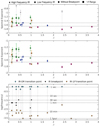 |
Fig. 9. Counterpart plots for Fig. 8, exponents plotted versus local plasma β. |
| In the text | |
Current usage metrics show cumulative count of Article Views (full-text article views including HTML views, PDF and ePub downloads, according to the available data) and Abstracts Views on Vision4Press platform.
Data correspond to usage on the plateform after 2015. The current usage metrics is available 48-96 hours after online publication and is updated daily on week days.
Initial download of the metrics may take a while.