| Issue |
A&A
Volume 683, March 2024
|
|
|---|---|---|
| Article Number | A114 | |
| Number of page(s) | 14 | |
| Section | The Sun and the Heliosphere | |
| DOI | https://doi.org/10.1051/0004-6361/202347975 | |
| Published online | 13 March 2024 | |
Magnetic power spectrum variability with large-scale total magnetic field fluctuations
Centre of mathematical plasma-astrophysics, KU Leuven, Leuven, Belgium
e-mail: This email address is being protected from spambots. You need JavaScript enabled to view it.
Received:
15
September
2023
Accepted:
20
December
2023
Abstract
Context. The Parker Solar Probe (PSP) is operational since 2018 and has provided invaluable new data that measure the solar vicinity in situ at smaller heliocentric distances than ever before. These data can be used to shed new light on the turbulent dynamics in the solar atmosphere and solar wind, which in turn are thought to be important to explain long-standing problems of the heating and acceleration in these regions. In recent years, it was realized that background inhomogeneities in magnetohydrodynamics could influence the development of turbulence and might enable other cascade channels, such as the self-cascade of waves, in addition to the well-known Alfvén collisional cascade. This phenomenon has been called uniturbulence. However, the precise influence of the background inhomogeneity on turbulent spectra has not been not studied so far.
Aims. In this work, we study the influence of background roughness on the turbulent magnetic field spectrum in PSP data, including data from encounter 1 up to and including encounter 14.
Methods. The magnetic spectral index αB receives our highest attention. Motivated by the presumably different turbulent dynamics in the presence of large-scale inhomogeneities, we searched for correlations between the magnetic power spectra and a measure for the degree of inhomogeneity. The latter was probed by taking the standard deviation (STD) of the total magnetic field magnitude after applying an appropriate averaging. The data of each PSP encounter were split into many short time windows, of which we subsequently calculated both αB and background STD.
Results. We find a significant impact of the background STD on αB. As the variations in the background become stronger, αB becomes more negative, indicating a steepening of the magnetic power spectrum. We show that this effect is consistent in all investigated PSP encounters, and it is unaffected by heliocentric distance up to 50 R⊙. By making use of artificial magnetic field data in the form of synthetic colored noise, we show that this effect is not simply due to the fluctuations imposed on the total magnetic field, but must have another as yet unidentified cause.
Conclusions. There is a strong indication that the background inhomogeneity affects the turbulent dynamics, possibly through uniturbulence. This leads to a different power spectrum in the presence of large-scale total magnetic field variations. The fact that it is present in all investigated encounters and at all radial distances up to 50 R⊙ suggests that it represents a general and ubiquitous feature of solar wind dynamics. The analysis with the synthetic colored noise indicates that the observed steepening effect is not to be attributed simply to the small-scale fluctuations superposed on the total magnetic field. This conclusion is confirmed by the fact that no similar consistent steepening trend is observed for the magnetic compressibility Cb instead of background STD. The steepening trend is instead a real physical effect induced by the large-scale variations in the background magnetic field.
Key words: plasmas / Sun: corona / Sun: magnetic fields / solar wind
© The Authors 2024
 Open Access article, published by EDP Sciences, under the terms of the Creative Commons Attribution License (https://creativecommons.org/licenses/by/4.0), which permits unrestricted use, distribution, and reproduction in any medium, provided the original work is properly cited.
This article is published in open access under the Subscribe to Open model. This email address is being protected from spambots. You need JavaScript enabled to view it. to support open access publication.
1. Introduction
Despite several decades of research, the precise mechanisms of coronal heating and solar wind acceleration are still not fully understood today. However, it is generally thought that the magnetic field plays a crucial role in the transportation and dissipation of the required amounts of energy (Schrijver & Zwaan 2000; Golub & Pasachoff 2009). It has been estimated that the necessary heating rates for active regions and coronal holes must be about 6 × 10⁻⁵ J/(m3s) and 8 × 10⁻⁶ J/(m3s), respectively (Narain & Ulmscheider 1990). Similar values, as well as a more detailed analysis of the problem, can be found in Aschwanden (2005). As the solar vicinity has been shown to be turbulent to a high degree (Bruno & Carbone 2013), many efforts have been made to explain the coronal heating problem through the concept of magnetohydrodynamic (MHD) turbulence (see, e.g., van Ballegooijen et al. 2014; Aschwanden 2005). The general picture is that energy in turbulent systems is injected at large spatial scales. As dissipation at these scales is insufficient to process all of the injected energy, an energy cascade develops that transfers the energy to systematically smaller spatial scales (Matthaeus & Velli 2011). From the nature of turbulence, it is clear that this energy cascade has to be driven by nonlinear interactions of the fluctuations. Only after this transfer of energy has reached the smallest scales of the cascade can efficient dissipation into heat occur. The exact nature of these fluctuations, as well as the manner in which they interact, strongly depends on the specific models used or assumptions made (Magyar & Nakariakov 2021). The simplest but nonetheless very widely used MHD formalism is that of idealized plasmas, implying incompressibility and homogeneity of the medium. Elsässer first showed that in this case, the basic MHD equations can be rewritten in a clear and symmetric way (Elsässer 1950). By rewriting in terms of  , now known as the Elsässer variables, the ideal MHD equations can be shown to take the following form:
 (1)
(1)
In the definition of the Elsässer variables, μ stands for the permeability of the medium and ρ is the mass density, which in ideal MHD is assumed to be constant both in space and time.
The Elsässer variables are useful not only because the ideal MHD equations can be rewritten in a simple way, but also for their interesting interpretation. When the medium through which the waves propagate can be assumed to be incompressible and homogeneous, the Elsässer variables represent purely outward- (z−) and inward- (z+) propagating Alfvén waves (Bruno & Carbone 2016; Magyar et al. 2017). Fast and slow magneto-acoustic waves, on the other hand, should be represented by a combination of the two Elsässer variables, even in a homogeneous medium (Magyar 2019).
Because turbulence is a highly nonlinear process, the equations in (1) must allow for nonlinear interactions. These originate from the advective derivative term on the left-hand side of the upper equation. For this term to be nonzero, we require the two Elsässer variables to have finite, nonzero values. This argumentation, together with the interpretation of the Elsässer variables in idealized media, led to the well-known scaling law of Iroshnikov (1964) and Kraichnan (1965). Now known as the IK scaling, this law states that E ∼ k−3/2, with E the energy and k the wave number. IK formalism regards magnetically dominated plasmas, in contrast to Kolmogorov theory, which considers purely hydrodynamic turbulence (Kolmogorov 1941). The Kolmogorov formalism follows the scaling E ∼ k−5/3, and despite its simplicity, it has proven to be widely applicable in a large number of experiments and studies, including many related to the solar wind. We provide examples of these experiments and studies below. The IK formalism of MHD turbulence was later revised by Goldreich and Sridhar (Goldreich & Sridhar 1995), who allowed for anisotropies in their model. Their theory, often referred to as the GS95 theory, yields different scaling laws for the directions along and perpendicular to the mean magnetic field. The former has a rather steep scaling following  , while the latter is in agreement with Kolmogorov scaling,
  . Boldyrev (2006) proposed an anisotropic scaling that reverts to the IK scaling in the perpendicular direction. This is the result of what they called “dynamic alignment”, meaning that fluctuations in the magnetic field and in the velocity field tend to align the directions of their polarizations. Measurements of magnetic field spectra close to the Sun generally tend to agree with IK formalism rather than with the Kolmogorov or GS95 scaling laws. However, it is unclear whether spectral anisotropy is observed, with various studies giving contradicting values for parallel spectra (Horbury et al. 2008; Telloni et al. 2019; Zhao et al. 2022a). For a more detailed description of all these turbulence theories, we refer to Schekochihin (2022).
Iroshnikov and Kraichnan identified the only nonlinear interactions of wave-like perturbations resulting from the ideal MHD equations to be those between counterpropagating Alfvén waves. In coronal loop structures, the existence of two populations of counterpropagating waves is ensured because the waves originate from the two footpoints of the loop. The waves are likely created through the convective flows in the photosphere, which cause random shuffling of the loop footpoints (Dahlburg et al. 2016; Van Doorsselaere et al. 2020). Furthermore, additional flux of Alfvénic waves can be created, for instance, by the internal acoustic modes of the Sun, as shown by Morton et al. (2019). These counterpropagating populations then meet each other along the loop and interact nonlinearly. However, in open field line regions such as those above coronal holes, counterpropagating Alfvénic turbulence can occur as well. Initially outward-propagating waves can under the right circumstances be reflected toward the Sun, thereby encountering other outward-traveling waves. It has been shown that this reflection can occur, for example, when there exists a gradient of the local Alfvén speed parallel to the mean magnetic field (Leroy 1980; Hollweg & Isenberg 2007).
As counterpropagating Alfvénic turbulence is perceived as (one of) the most dominant mechanism(s) of turbulence in the solar atmosphere and solar wind, numerous models have been developed to study coronal heating due to this type of turbulence in both coronal loops and open field line regions. For example, Matthaeus et al. (1999) described a mechanism according to which outward-propagating Alfvén waves reflect and interact, thus generating turbulent decay. The authors argued that the reflection rate R strongly affects the efficiency of heat production. For realistic values of R ≥ 1, they found that almost half of the input energy is dissipated into heat. This reflection rate is approximated as R ∼ VA/Δ, with VA the local Alfvén speed and Δ the typical scale height for changes in the Alfvén speed. Chandran & Perez (2019) described transverse incompressible MHD fluctuations in a narrow magnetic flux tube, representing an open field line region. Their model matches observational constraints fairly well, especially for distances greater than 1.3 R⊙, and it is consistent with the idea that MHD turbulence can account for most of the heating of the fast solar wind. These models are just two examples out of many others, but a general conclusion is that MHD turbulence can maintain a corona of multimillion degree Kelvin, while balancing radiative cooling and conductive losses (Van Doorsselaere et al. 2020).
Due to the necessity for reflected waves in MHD turbulence theories, inhomogeneities along the mean magnetic field are widely used in numerical modeling. Variations perpendicular to the mean magnetic field, on the other hand, are far more often neglected, despite ample evidence for large variations in the solar vicinity (Raymond et al. 2014; Borovsky 2020). One counterexample is the work of Evans et al. (2012), who investigated the effects of surface Alfvén wave (SAW) damping in regions with gradients in the local density, and therefore also in the Alfvén speed, perpendicular to the magnetic field. Magyar et al. (2017) argued that in the case of inhomogeneous plasmas, MHD waves display mixed properties of the waves encountered in homogeneous MHD (Alfvén, fast, and slow). A more elaborate explanation of what this mixing implies mathematically can be found in Goossens et al. (2019). In general, no pure Alfvén or pure magneto-acoustic modes exist any longer in inhomogeneous media, although a propagating wave can still be predominantly Alfvénic or magneto-acoustic. These modes are referred to variously as surface Alfvén, kink, or Alfvénic waves (in the following, we use Alfvénic). An important consequence is that Alfvénic modes can no longer be described by one Elsässer variable alone. Instead, just like the magneto-acoustic modes, they have to be described by a combination of both z− and z+. However, even in an inhomogeneous medium, the Elsässer variable representing the direction of the wave propagation will be strongly dominant. The exact relative amplitude of the two Elsässer components in the representation of the propagating wave is thought to be dependent on the precise degree of inhomogeneity and other plasma parameters.
This change in the representation of Alfvénic waves can have a profound impact on the process by which the turbulent cascade proceeds. In order for the advective derivative term in Eq. (1) to be nonzero, both Elsässer variables still need to have a nonzero value, but now this requirement can be fulfilled by Alfvénic waves traveling in only one direction. Because Alfvénic waves in a perpendicularly inhomogeneous medium are described by both z− and z+, they can cause a cascade of energy without the need of a counterpropagating population of waves. Magyar et al. (2017) and Magyar (2019) performed 3D MHD simulations of a perpendicularly inhomogeneous plasma penetrated by outward-propagating Alfvénic waves. It was shown that even in this unidirectional propagation, the nonlinear self-deformation of waves can lead to a cascade of energy to systematically smaller spatial scales. This phenomenon is now known as “uniturbulence”. At the time of writing, relatively little is known about uniturbulence. Its typical characteristics are unclear, as is whether it obeys the same scaling laws as other turbulence mechanisms, or how important it is with respect to these other mechanisms, such as counterpropagating Alfvénic turbulence in the solar atmosphere and solar wind. It is also uncertain how uniturbulence could be recognized in real data. Magyar & Nakariakov (2021) concluded from 3D compressible MHD simulations that turbulence features do not seem to display differences between the two mechanisms discussed above. However, it would seem plausible that when variations perpendicular to the mean magnetic field become stronger, uniturbulence becomes increasingly important. The aim of this work is to use data of the Parker Solar Probe (PSP) close to the Sun to investigate whether an increase in background variations has a systematic impact on the overall turbulent motions in the solar wind. The main feature of interest for this work is the spectral index of the magnetic field power spectrum αB. If this variable can be shown to change significantly with different values of background magnetic field variations, this might indicate a dependence of turbulent dynamics on the background inhomogeneity, and it may represent a first discovered indication of uniturbulence in PSP data.
Prior to this work, several other authors already investigated the rates of turbulent energy cascade in the solar wind. For example, Goldstein et al. (1995) used Ulysses data to investigate z± power spectra at large heliographic latitudes and distances between 2 − 4 AU. They found spectral indices of −5/3, in agreement with the Kolmogorov or GS95 theory. Podesta et al. (2006) used data from the Wind spacecraft to show that at 1 AU, proton velocity field power spectra tend to agree with the IK formalism (α ≈ −3/2), while magnetic field power spectra generally have steeper slopes with α ≈ −5/3. These results were later confirmed, for example, by Tessein et al. (2009), using data from the ACE and Helios 1 missions at 0.3 − 1 AU. More recently, PSP data allowed similar studies for distances much closer to the Sun. By analyzing these data, it has by now become clear that the magnetic field power spectra close to the Sun (a few tens of R⊙) differ considerably from those measured around 1 AU. Kasper et al. (2021) analyzed data from the eighth PSP encounter, which is the first time the probe entered regions of Alfvénic Mach numbers below unity, and recovered to a very good agreement an IK slope of k−3/2 for αB. This scaling was valid in an inertial range of 2 × 10⁻³ Hz up to about 3 × 10⁻¹ Hz. Sioulas et al. (2023) found the same −3/2 slope for PSP data close to the Sun, independent of the plasma parameters. However, with increasing heliocentric distance, the authors showed that this slope steepens toward a Kolmogorov or GS95 scaling of k−5/3. A similar steepening of the magnetic spectral index was found by Zhao et al. (2022b), who also reported a clear correlation between heliocentric distance and the angle θBR between the radial direction and the mean magnetic field. As the heliocentric distance increases, the mean value of θBR increases as well. Therefore, the authors concluded that it is uncertain whether the observed variation in magnetic spectral index is due to the radial distance variations or to the sampling direction of the spacecraft. On the other hand, Sioulas et al. (2023) reported that they did not find a similar correlation between the magnetic spectral index and the field-flow angle ΘBV using a global magnetic field. While this appears to be a strong disagreement between the two authors, this may not necessarily be the case because the exact physical meaning of θBR could be expected to differ from that of ΘBV. Sioulas et al. (2023) also found the inertial range to extend toward lower frequencies as the probe moves away from the Sun. Additionally, they concluded that this steepening trend is less efficient for the fast solar wind than for slow wind. At a distance of 1 AU, the former agrees with the Kolmogorov slope, while the latter shows a steeper spectrum of αB ≈ −1.8. Finally, highly Alfvénic intervals tend to steepen much more moderately than intervals of low Alfvénic content. The degree of Alfvénicity is in general interpreted by how closely the cross helicity approaches unity and how close the normalized residual energy is to zero. Sioulas et al. (2023) suggested that these results may indicate a positive correlation between the solar wind speed and Alfvénicity.
A very similar steepening of the magnetic power spectrum from −3/2 toward −5/3 with increasing heliocentric distance was obtained by Shi et al. (2021), using data of the first five PSP encounters. They also show that no such steepening trend is present in the velocity field power spectra, which remain at a constant IK slope of −3/2, regardless of the heliocentric distance. This agrees with the findings of Chen et al. (2020), who made use of data from the first two PSP encounters alone. They showed that close to the Sun, the dynamics are dominated by outward-propagating waves of high Alfvénicity, but that this dominance decreases with radial distance from the Sun. Shi et al. (2021) also confirmed the previously mentioned suggestion of Sioulas et al. (2023) by showing that the fast solar wind has a statistically significant higher Alfvénicity than the slow wind. However, additional factors can cause the turbulence properties to vary significantly even between winds of similar velocities. For example, slow wind originating near polar coronal holes has been shown to have a much lower Alfvénicity than slow winds coming from active regions and pseudo-streamers (Shi et al. 2021). For more details on the Alfvénicity of slow winds, we also refer to d’Amicis et al. (2021).
In a recent paper, Dunn et al. (2023) investigated the influence of spherical polarization on the spectral index of the magnetic power. They identified deviations from spherical polarization to be compressive fluctuations, that is, changes in |B|, and concluded that they strongly affect the turbulent scaling laws. In the absence of compressive fluctuations, shallow spectra of k−3/2 are found, while a steepening toward k−5/3 is reported in regions with stronger compressive fluctuations. When fluctuations are dominated by discontinuities, even a power-law scaling approaching k−2 was found. After these discontinuities were numerically removed, the spectral index approached −3/2 again, indicating that the observed steepening is indeed attributable to a strong discontinuity. The severity of the fluctuations is quantified by means of the perpendicular variance isotropy ψ, which probes the relative power in the variations along the maximum and minimum variance directions perpendicular to the mean magnetic field. Therefore, no variations parallel to the mean magnetic field are taken into account in the calculation of the degree of fluctuations. It is not mentioned in the paper whether this implies that the recovered spectral index values are applicable to k⊥ rather than to k∥. McIntyre et al. (2023) used data from PSP encounters 1 up to 11 to investigate the influence of several parameters on the spectral index of the magnetic power. Their statistical analysis enabled a rigorous individual separation of the variation in αB with each parameter. They reported that the transition from αB ≈ −3/2 close to the Sun to αB ≈ −5/3 farther away occurs about 50 R⊙. They also investigated potential influences of cross helicity, residual energy, solar wind velocity, magnitude of magnetic field fluctuations and turbulence age, which is a parameter that approximates the number of nonlinear times passed over the outward propagation of a parcel of plasma from the Sun. This parameter could be expressed as τnl = λ/δb, with λ the scale of the fluctuation, and δb the perturbation of the magnetic field in velocity units. McIntyre et al. (2023) described the calculation of these quantities in more detail in their paper. Of all the investigated parameters, the cross helicity σc was found to have the most impact on the magnetic spectral index by far. At low values of σc (≈0 − 0.5), αB agrees with a Kolmogorov scaling, while at larger σc, the power spectrum gradually flattens toward IK scaling, regardless of the heliocentric distance. For all other parameters, including the variability in the magnetic field strength, the evidence of an underlying cause for spectral index variability was reported to be weak.
Although these studies firmly established several trends in the magnetic spectral index αB with different factors, none of them specifically investigated the influence of variations in the mean background magnetic field. This is the primary topic of this work. After elaborating on the employed data in Sect. 2, we discuss our results in Sect. 3. Our main conclusions are summarized in Sect. 4.
2. Data
Two types of data were used for the calculations in this work: magnetic field data, and radial heliocentric distance data. The magnetic field data were downloaded from the NASA Coordinated Data Analysis Web (CDAWeb). These data were measured by the fluxgate magnetometers (MAGs), which are part of the Electromagnetic Fields Investigation (FIELDS) instrument of PSP (Fox et al. 2016). The magnetic field data provided by the MAGs can be downloaded in spacecraft coordinates (x, y, z) or in radial-tangential-normal coordinates (r, t, n). Furthermore, they are available at their full fast cadence of 292.97 Hz or downsampled to either one minute or to 4.58 Hz (Bale et al. 2016). For practical reasons, we used the latter option for both the coordinate system and for the cadence choice. The data were downloaded in the form of .cdf files, which were readily converted into Python variables. The number of NaNs in the downloaded data varied over different PSP encounters. For several encounters, it was simply zero, for others, it was as high as 1000 NaN data points. However, for every PSP encounter, 12 days of data were included, so that at a cadence of 4.58 Hz, this still resulted in fewer than 0.025% of the data points being NaNs. Therefore, the data were still considered to be reliable.
The coordinate data were downloaded through the Spacecraft, Planet, Instrument, C-matrix, and Events (SPICE) kernels of NASA. SPICE is an information system built by the Navigation and Ancillary Information Facility (NAIF). It is meant to help visualize scientific observations and mission development. These kernels can be readily used to extract the radial, tangential, and normal position of the PSP at high precision throughout the duration of the mission. In this work, we only use the radial position data for the periods of perihelion passages.
3. Results and discussion
3.1. Spectral index analysis
In order to investigate possible trends between the magnetic spectral index and background magnetic field variations, the data of one whole encounter must be split into many shorter time windows. The spectral indices and background variations of all these time intervals can then be calculated separately, and a potential correlation between them can be identified. However, a trade-off has to be made in the decision of how wide these time windows should be. When they are taken too small, these time windows will contain too few data points for an accurate determination of the spectral index, which will therefore be prone to random fluctuations. When they are taken too large, these random fluctuations will surely be erased, but episodes of strong background variations will be mixed with periods of quiet background environments, thus jeopardizing the results. In an attempt to find a suitable middle ground between these extremes, we opted to divide the total encounter data into time windows of 6 min. This is comparable to Bandyopadhyay et al. (2022), for example, who chose to split PSP data into intervals of ≈10 min, and who computed the variance anisotropy Ab in each of them separately. Our choice for 6-min time windows was primarily based on a trial-and-error method, where we also considered wider intervals of 30 and even 60 min. However, the results from these larger windows were of noticeably lower quality, and they were therefore omitted. We mean by lower quality that the obtained correlation between the magnetic spectral index and variations in the background magnetic field was weaker or even totally absent. We also chose to capture the degree of the background variations by means of the standard deviation (STD) of the background total magnetic field magnitude, |B0|. This background was obtained by an appropriate averaging over time. We elaborate on this averaging below.
Figure 1 shows the variation in the magnetic spectral index αB versus STD of |B0| for 12 days of data surrounding the 12th encounter of PSP. These spectral indices were obtained by fitting a linear function through the log-log power spectrum of all the 6-min time intervals separately. The frequency range taken into consideration in the production of this linear fit was that between 10−2 − 10−1 Hz. This frequency regime is comfortably well situated inside the inertial range, as was also verified by Kasper et al. (2021). The slope of this linear fit in log-log space then equals the spectral index α. Using a sliding step of one-tenth of the time window, that is, ≈36 s, a total of over 28 700 spectral indices were calculated for a single PSP encounter. The uncertainties on these indices originate from the covariance matrix of the linear fits, and they are drawn as green error bars in Fig. 1. In the calculation of the STD values of Fig. 1, the raw magnetic field was first divided by a one-hour average to subtract the large-scale envelope shape of B. The raw total field and its one-hour average are illustrated in the top panel of Fig. 2 for clarification. After dividing the raw field by this one-hour average, we obtained a signal that was normalized to unity, as shown by the blue line in the lower panel of Fig. 2. Subsequently, a five-minute average was taken of this ratio, shown by the red line. It is this red signal that we proceed with in the analysis, and it is this red signal that we divide into the six-minute time windows and subsequently calculate the STD of. The purpose of dividing the raw signal by its one-hour average is to normalize it with respect to the heliocentric distance. This ensures that the results of this work are not just indirectly reproducing those of Sioulas et al. (2023), for instance, who showed that the magnetic field power spectrum steepens with increasing heliocentric distance from αB = −3/2 at r ≈ 13 R⊙ toward αB = −5/3 at r ≈ 220 R⊙. The purpose of the subsequent averaging over 5 min is to ensure that we searched for variations in the total magnetic field magnitude at scales larger than the perturbation scales that were used to obtain the power spectrum, variations that in this sense represent background variations. A decreasing trend of αB with increasing STD is observed in Fig. 1, indicated by the red linear fit through the data. A weighted least-squares (WLS) analysis indicates that this trend is a relatively small effect (R2 ∼ 0.01), but nonetheless, it is statistically highly significant (P < 0.001). This R2 value means that the variation in the background magnetic STD can account for about 1% of the variation in αB. This relatively low value is expected because the spreading of αB values in Fig. 1 is strong, even for very similar values of the background magnetic STD. However, the recovered P-value indicates that if the background STD values were to affect αB not at all, the chance of recovering the trend in Fig. 1 would be only 0.1%. This chance is clearly negligible, so that we can conclude a certain influence of the background magnetic STD on the spectral index of the magnetic power.
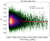 |
Fig. 1. Magnetic spectral indices αB vs. STD of the background magnetic field for the 12th encounter of PSP. |
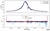 |
Fig. 2. Extraction of the measure for the background STD from the data. |
An important remark to make here is that although we divided the total encounter data into relatively short time windows of 6 min, large-scale structures such as Heliospheric Current Sheet (HCS) crossings or strong discontinuities may still exist in some windows. As we have taken the spectral index of the raw total magnetic signal, no measures were taken to remove the impact of these structures on the value of αB. Some values displayed in Fig. 1 may therefore very well be influenced by them. However, due to the double averaging (first over one hour and subsequently over 5 min) performed on the data prior to the STD calculation, the impact of these large-scale structures on the STD values can be presumed to be strongly damped if not totally erased. As a consequence, possible correlations between αB and background STD that are purely due to these structures are also neutralized. The observed downward trend in Fig. 1 is therefore not at all to be attributed to influences of these large-scale discontinuities.
3.2. Consistency over PSP encounters
Although only the result for the 12th encounter of PSP was visualized in the previous section, similar results were obtained for all other PSP encounters performed so far. At the time of writing, the employed magnetic field data is publicly available for encounter 1 up to and including encounter 14. All according figures can be found in Appendix A. All these figures display a decreasing trend of αB with increasing background magnetic field STD. In all of the figures in the Appendix, as well as in Fig. 1, the maximum of the x-axis was taken to be one-seventh of the overall maximum of the measured STD values in order to remove extreme outliers from the plots. The feature of interest is now the slope of this decreasing trend, and whether its deviation from zero is statistically significant. We henceforth refer to this slope as γ to avoid any confusion with the slopes of the individual power spectra, which are the spectral indices α. Just as for α, we determined the value of γ by fitting a linear function through the individual data points, as was done in Fig. 1, and computed the uncertainty on this value by means of a covariance matrix. An important difference is that for the determination of γ, we took the uncertainties on all αB into account by applying weights wi = 1/σi, with σi the uncertainties on αB. This procedure logically influences the obtained uncertainty on γ itself. In Fig. 3 we show the resulting values of γ for all 14 PSP encounters with the accompanying error bars.
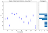 |
Fig. 3. Slope γ of the decreasing trend in the spectral index with increasing magnetic field STD for encounters 1 up to and including 14. A histogram is added to better visualize the distribution of the γ values in all encounters. |
Clearly, the decreasing trend of αB with increasing background magnetic STD is consistent in all PSP encounters. The obtained uncertainties are also sufficiently small for all data points to be multiple standard deviations below zero. Therefore, this decreasing trend is a statistically significant effect, with a P-value below 0.001, and it is generally present and observable during all PSP encounters. The mean value of γ in all encounters is ≈ − 4.3, with a variance of about 1.05. To better visualize this distribution, a histogram is added to the figure. However, the relatively small error bars on the γ values also cause the data points to lie outside the respective 1σ uncertainty intervals. This variation could be due to a wide range of factors: the exact position of the probe during the encounter, the solar wind speed, and the HCS influence and variation over the solar cycle could all be considered to potentially influence the trend.
Instead of taking the STD of an averaged magnetic field, a more common measure for relative variability in literature is the magnetic compressibility, defined as Cb = (δ|B|/|δB|)2 (Bale et al. 2019). This quantity describes the ratio of the magnitude fluctuations in the magnetic field and the total magnetic trace fluctuations (Zhao et al. 2022c), both relative to some averaged reference. Cb is often used as a proxy for Alfvénicity and has been shown to increase with radial distance (Chen et al. 2020; Bale et al. 2019; Telloni et al. 2021). However, there is a fundamental difference between this quantity and the STD measure that was used in the production of Fig. 1, for instance. Whereas the former essentially measures deviations of a pure signal with respect to some time-averaged signal, the latter probes variations in the time-averaged signal itself. We performed an analysis similar to the analysis that led to Fig. 1, but considered magnetic compressibility instead of the background magnetic STD. In doing so, the reference relative to which the deviations are to be calculated was taken to be a 5-min average to maintain the analogy with the background STD calculation. In contrast to the findings of Dunn et al. (2023), we found no consistent trend of the spectral index with increasing compressibility from this analysis, as the values for γ were positive for some encounters, but negative or approximately zero for others. One possible explanation for the discrepancy between our findings and those of Dunn et al. (2023) is the different computation of the compressibility. Whereas we took the averaged reference to be over a constant length of 5 min, Dunn et al. (2023) used a more dynamic approach in which the length of the interval was set to ten times the correlation time TC(t), which in turn is defined as the time over which the autocorrelation function C(τ) drops below a value of 1/e. This results in an average length of 7092 s for the intervals, which is longer by an order of magnitude than the 5-min averages used in this work. It is therefore reasonable to assume that these two measures for the compressibility have different physical interpretations. We can interpret Cb as computed in this work as describing the average power of small-scale compressible waves, while in the work of Dunn et al. (2023), it probes the energy residing in more large-scale features of the solar wind. Following this argumentation, we conclude that small-scale waves traveling through the solar wind do not induce any steepening effect of αB themselves. The cause for the observed steepening instead lies in the variation in the background medium itself. Whether this steepening effect is indeed the same as the effect found by Dunn et al. (2023) depends on how closely our measure of the background magnetic field STD is correlated to their measure for magnetic compressibility. We did not study this in this work. For completion, we should add to this that we also considered evaluating the magnetic spectral index as a function of |B|/|B0|, where |B0| denotes the average magnetic field strength, although no STD calculation entered the analysis here. Again, we found no steepening effect of αB with this parameter like the effect we found with the background magnetic field STD.
3.3. Consistency over heliocentric distances
It might be argued that the variations in the background magnetic field become stronger at smaller heliocentric distances even when the large-scale envelope shape is subtracted before the STD values are computed. If this were true, heliocentric distance could still affect our results, and we would be measuring a steepening effect of the magnetic power spectrum over decreasing heliocentric distance. In order to disprove this argument, we performed a similar analysis as before, but now taking the data of all encounters together and disentangling different heliocentric distance regimes instead. One of the resulting plots is shown in Fig. 4. The data considered for the production of this figure originate from all 14 PSP encounters, but only consider the time intervals during which the probe traveled between 20 and 30 solar radii. It is clear that even for comparable distances, an increase in the background magnetic field STD leads to an overall decrease in the spectral index of the magnetic field power. For completeness, we should add here that in the production of this plot, no data of the first three PSP encounters were used because these encounters did not bring the probe closer than ≈35.6 R⊙. The linear fit through the data in Fig. 4 seems to be considerably steeper than the fit in Fig. 1, but this is merely due to a difference in the included x-axis range. When these ranges were to be equalized between the two figures, the slope of the fits would be seen to be very similar (see Figs. 3 and 5). Just as before, the maximum value on the x-axis for each figure was taken to be one-seventh of the overall maximum of the calculated STD values, so that extreme outliers were excluded from the plots.
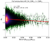 |
Fig. 4. Magnetic spectral index αB vs. STD of the background magnetic field for PSP encounters 1–14 for time windows in which the position of the PSP was between 20 and 30 R⊙. |
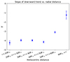 |
Fig. 5. Slope of the decreasing trend of the spectral index with increasing magnetic field STD for different distinct intervals of the heliocentric distance. The data taken into consideration consist of PSP encounters 1–14, with 12 days of data per encounter. |
The procedure leading to Fig. 4 was applied to all relevant distances in bins of 10 R⊙. The values of γ with corresponding uncertainties were again calculated by a linear fit and accompanying covariance matrix, taking the inverse of the uncertainties on αB as weights in the calculation. The result is shown in Fig. 5. The values of the first four distance bins, up to 50 R⊙, are close to −4 and lie within the respective 1σ uncertainty intervals. At larger heliocentric distances, the trend flattens, with γ being −3.1 ± 0.1 for 50 R⊙ < r < 60 R⊙ and −1.2 ± 0.4 for 60 R⊙ < r. However, the reliability of this last data point is somewhat questionable because this distant regime includes far fewer data points for the 12 days surrounding every PSP perihelion passage than the other distance regimes. Therefore, the spectral indices could be determined less accurately, so that the uncertainties on αB are larger. The remarkably larger error bar on γ of this data point is a first consequence of that. A second consequence is that the linear fit through the αB data points of this regime did not have a P-value of P < 0.001, as was the case for the other distance bins. For 60 R⊙ < r we instead have P < 0.06. The according figure is shown in Appendix B. At these large distances, multiple effects are worth consideration to explain why the steepening effect becomes weaker. First, the magnetic field power spectrum begins to steepen (Sioulas et al. 2023), so that even at zero STD, the spectral index is more negative than −3/2. This is shown in the last figure of Appendix B, where the linear fit is at a value of −1.59 already at zero STD. This logically diminishes the value of γ. It is very well possible that this steepening sets in around 50 R⊙ because this was also found by McIntyre et al. (2023). Second, at large radial distances, cross helicity influences the spectral index values considerably, so that an IK slope of –3/2 becomes difficult to recover altogether (McIntyre et al. 2023). All figures leading to the data points in Fig. 5 strongly resemble the result of Fig. 4, and they can be found in Appendix B.
With the observed steepening trend of αB firmly established for all PSP encounters and all heliocentric distances up to 50 R⊙, we can turn to the question of which physical phenomenon is behind it. It is difficult to determine with certainty whether this steepening trend is attributable to an increasing importance of uniturbulence. It is, however, a rigid result that does not seem to be simply due to some isolated event. The fact that a similar trend is observed for all investigated encounters suggests that it is a manifestation of an intrinsic feature of solar wind turbulence that is not susceptible to environmental conditions that may vary between PSP visits. Therefore, uniturbulence seems to be at least one plausible candidate to explain the observed trend, as it is anticipated to be a ubiquitous phenomenon in the solar atmosphere and solar wind.
3.4. Artificial noise verification
As the data used to produce Fig. 1 and the other figures in Appendix A are limited to magnetic field data, some characteristic feature of these data must cause the observed steepening effect. In an attempt to retrace this source of the slope variability, three samples of artificial colored noise were generated with the same length as the actual magnetic field components for one single encounter. The slope of the power spectra of these artificial data samples was chosen to be −3/2, just like the actual magnetic field components. This was done using the Python package colorednoise, which is able to generate Gaussian-distributed noise with a power-law spectrum of arbitrary exponents. Logically, the power spectrum of the total (vectorial) sum of the artificial components will also have the same −3/2 slope.
In addition, the total (vectorial) amplitude of the actual magnetic field data was mimicked by the generated set of artificial noise. In this way, the fluctuations in the total magnetic field were also copied indirectly. This was done by linearly scaling up the three artificial components until their total magnitude matched the real magnetic field magnitude, while simultaneously keeping the ratio of the magnitudes of the components unchanged. The artificial data are visualized in Fig. 6, in which the copied magnitude is that of encounter 13. The mimicking of the total magnetic magnitude causes the artificial data to follow the typical large-scale envelope shape over the encounter. More detailed features such as HCS crossings are not carried over to the artificial data.
 |
Fig. 6. Three samples of artificial colored noise, mimicking the actual magnetic field data. |
If now a similar downward trend of spectral index were recovered for these artificial data, then the fluctuations in the total magnetic field could be successfully held accountable for causing this trend. When performing the same analysis as led to Fig. 1 on the data of Fig. 6, we obtained the result of Fig. 7. It is clear that no downward trend of the spectral index is recovered similar to that in the real data, so that γsynth ≈ 0. Due to the random nature of this synthetic data, the exact value of γ could logically vary somewhat between several runs. However, the mean value over the runs was approximately zero, and in no case was a value for γ as negative as those in Fig. 3 recovered for the synthetic data. Therefore, it seems that the manner in which the total magnetic field fluctuates does not itself cause the downward trend in the spectral index. This should not be viewed as a negative result, however. If the opposite were true, and we would recover a similar trend while using a sample of artificial noise as simple as that in Fig. 6, then we should seriously consider the possibility that this trend is simply some artifact of the performed data analysis without any involved physics. Our results indicate that there must instead be an underlying physical feature of the magnetic field data that is the cause of the observed steepening effect, which must have a real physical origin.
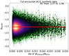 |
Fig. 7. Variation in the spectral index αB as a function of background STD for the artificial colored noise illustrated in Fig. 6. No downward trend is recovered. |
3.5. Kurtosis analysis
One such origin we considered as the cause of the observed trend is intermittency. The notion of intermittency refers to the property of turbulent systems that fluctuations tend to become increasingly sparse in time and space at smaller scales (Beresnyak & Lazarian 2019). This property is neglected in theoretical scaling laws such as Kolmogorov or IK scaling, which rely on the principle of self-similarity. As the name suggests, this principle implies that turbulent characteristics are similar at all scales within the inertial range, or equivalently, that the spatial distribution of the turbulent eddies look the same on any scale level throughout the inertial range (Biskamp 2003). The violation of strict self-similarity by intermittency has been shown by both numerical simulations and experiments. At the dissipation scales, the breakdown of self-similarity causes non-Gaussian dissipation structures, as elaborated by Biskamp (2003). As these deviations from Gaussian shape will logically translate into a nonzero value for the kurtosis of the distribution, we probe in this part of the analysis the intermittency of the solar wind by means of the kurtosis of the magnetic field components.
Wang et al. (2023) recently investigated the effect of intermittent structures on the magnetic power spectral index in the slow solar wind by analyzing data from the Wind spacecraft between 2005 and 2013. They constructed a parameter Imax that quantizes the level of intermittency at a timescale of τ = 24 s over a duration of 5–6 min. They reported that as this parameter increases, indicating a stronger intermittent environment, the magnetic spectral index decreases significantly, from −1.63 to −2.01. They added to this finding that during these intermittent periods, no significant influence of compressibility on the spectral index was found. The reported results of this paper convincingly establish the impact of intermittency on the spectral index. If intermittency is in any manner correlated to the measure of background inhomogeneity used in this work, then maybe we would have indirectly reproduced the results of Wang et al. (2023).
In order for intermittency to cause the steepening trend observed in this work, there must exist a correlation between the variations in the background magnetic field and the kurtosis values of the magnetic components. In Fig. 8, we attempt to find this correlation by plotting the kurtosis of the radial magnetic field component as a function of the STD values of the background magnetic field. To create this figure, only data of the seventh PSP encounter were used, which was split into time intervals of one hour. These time windows were shifted over 5 min. The background was obtained through averaging over 5 min, and in this case, no cancellation of the large-scale envelope shape was performed. It is clear from the scatter plot that there is no obvious correlation, as the data points are scattered randomly over the frame. Nonetheless, a linear fit was made through the data, the slope and offset of which are indicated in the legend of the figure. An ordinary least-squares (OLS) linear regression analysis indicates that this fit has no statistical significance, as its R-squared value does not exceed 0.001 and the P value amounts to 0.846. Similar results were also obtained when regarding the kurtosis values of the other magnetic field components. Having no clear relation between background STD and component kurtosis at hand, we have no substantiated reason to believe that the amount of variation in the background has a significant impact on the degree of intermittency in the magnetic field signal. Therefore, we cannot motivate any potential role for intermittency in the observed steepening trend either. It is more likely that the feature in the magnetic field data that causes the steepening trend resides in one of the higher-order moments of the distribution. This kurtosis-related analysis is a rather superficial verification of whether intermittency is likely causing the trend, however. To exclude any intermittent influence with certainty, a more rigorous study is required. This study would preferentially include a partial variance of increments (PVI) analysis as well. PVI was not included into this work mainly due to time constraints, but the possibly different conclusions resulting from such a study is very interesting for future work.
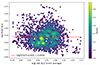 |
Fig. 8. Kurtosis of the radial magnetic field component vs. the STD of the total background magnetic field. |
4. Conclusion
We investigated the change in the magnetic power spectral index αB with the degree of variation in the background magnetic field. The background field was obtained by averaging over 5 min, and the large-scale magnetic field envelope shape was erased by dividing the raw field by a one-hour average. The degree of variation was then captured by taking the STD of 6-min time intervals, which were shifted by leaps of 36 s. We found that the spectral indices of these 6-min time windows became significantly more negative with increasing STD values. Moreover, although we applied an averaging over 5 min before calculating the STD values for all results included into this report, we also performed similar tests with other averaging time frames. Averaging over 15 and 30 min was tested as well, and while this sometimes yielded similar results, the plots originating from a 5-min averaging window were clearly superior.
At negligible STD values, we measured a mean value for αB of −3/2, in agreement with previous studies of PSP data close to the Sun (see, e.g., Sioulas et al. 2023; Shi et al. 2021; McIntyre et al. 2023). When the background STD values become higher, the magnetic power spectra of the 6-min time windows steepen toward αB ≈ −5/3 and even steeper, as shown in the figures in Appendices A and B. The rate of this steepening effect was captured by the slope γ of a linear fit to the data. We showed that γ is significantly different from zero, and that it is negative for PSP encounters 1 up to and including 14 separately. For every encounter, we took the data of the 12 days surrounding the perihelion passage into account. We also showed that the decreasing trend of αB with the background magnetic field STD is independent of heliocentric distance, at least up to r ≈ 50 R⊙. This was done by considering the data of all 14 encounters simultaneously and differentiating between distinct regimes of heliocentric distance instead. It was shown that the γ values for the distance intervals up to r ≈ 50 R⊙ agree at a value of about −4, while for larger distances, the value of γ approaches zero.
Artificial colored noise was generated with a −3/2 slope for its power spectrum, as is the case for the magnetic field. Additionally, the synthetic data were made to mimic the total (vectorial) amplitude of the magnetic field. A similar analysis with these synthetic data did not result in a similar steepening effect of the spectral index. We concluded that the fluctuations on the total magnetic field therefore do not directly cause this steepening effect.
With the theoretical motivation for this work in mind, it seems that uniturbulence is at least a probable candidate for explaining this steepening effect. It is known from previous MHD simulations that when variations in the medium perpendicular to the mean magnetic field become strong, uniturbulence gains importance. As uniturbulence could provide an additional cascade rate to the other turbulence mechanisms present (e.g., counterpropagating Alfvénic turbulence), energy could be dissipated faster. Therefore, the steepening of the magnetic power spectrum with increasing STD values may be interpreted as a manifestation of an increasing dominance of uniturbulence in solar wind dynamics. The fact that the steepening effect is present for all investigated PSP encounters and that it is indifferent to heliocentric distance (up to r ≈ 50 R⊙) further strengthens this claim. It is to be expected that at much larger distances from the Sun, inhomogeneities become weaker, so that the influence of uniturbulence becomes less pronounced in the turbulent dynamics. One possible caveat in this reasoning about uniturbulence is the fact that we did not appropriately distinguish between variations across and along the mean magnetic field in this work, although uniturbulent motions are considered to be created by perpendicular variations alone. However, at the time of writing, we are not aware of any other mechanism that can at least partly explain this omnipresent steepening effect of αB in the solar vicinity.
When applying the ideal IK scaling law to real solar wind data, we recall that some refinements have to be made in order to obtain the following, more realistic scaling law:
 (2)
(2)
In this equation, f(d, v, σc) stresses the fact that the exact value of the exponent depends on the heliocentric distance d, the speed of the solar wind v, as shown by Sioulas et al. (2023), for example, and also on the cross helicity σc, as shown by McIntyre et al. (2023). The factor f(𝒱bg) empathizes the main result of this work, namely that background variations (symbolized here by 𝒱bg) also have a considerable impact on αB. Future work is highly desirable, most importantly, to further constrain the observed steepening effect. More extensive investigations could quantify this effect and thereby determine the exact form of f(𝒱bg), which was not done in this work (we implicitly assumed that f(𝒱bg) is a linear effect by fitting a linear function through the data, but even this is open to debate). Studies like this, which might also include data from other probes, could also investigate possible variations in this steepening trend with the latitude of the measured solar wind, or with the phase in the solar cycle. Second, follow-up work is also necessary to better isolate the feature in the magnetic field data that causes the steepening trend. More sophisticated modeling techniques with accordingly more advanced types of artificial data could be of great use for this purpose.
Acknowledgments
N.M. acknowledges Research Foundation – Flanders (Fonds voor Wetenschappelijk Onderzoek (FWO) – Vlaanderen) for their support through a Postdoctoral Fellowship. T.V.D. was supported by the C1 grant TRACEspace of Internal Funds KU Leuven and a Senior Research Project (G088021N) of the FWO Vlaanderen. This research was supported by the International Space Science Institute (ISSI) in Bern, through ISSI International Team project #560.
References
- Aschwanden, M. 2005, Physics of the Solar Corona: An Introduction with Problems and Solutions (Springer Berlin Heidelberg) [Google Scholar]
- Bale, S., Goetz, K., Harvey, P., et al. 2016, Space Sci. Rev., 204, 49 [Google Scholar]
- Bale, S., Badman, S., Bonnell, J., et al. 2019, Nature, 576, 237 [Google Scholar]
- Bandyopadhyay, R., Mattaeus, W., McComas, D., et al. 2022, ApJ, 926, 6 [NASA ADS] [CrossRef] [Google Scholar]
- Beresnyak, A., & Lazarian, A. 2019, Turbulence in Magnetohydrodynamics (Berlin, Boston: De Gruyter) [CrossRef] [Google Scholar]
- Biskamp, D. 2003, Magnetohydrodynamic Turbulence (Cambridge University Press) [Google Scholar]
- Boldyrev, S. 2006, Phys. Rev. Lett., 96, 115002 [Google Scholar]
- Borovsky, J. 2020, Front. Astron. Space Sci., 7, 20 [NASA ADS] [CrossRef] [Google Scholar]
- Bruno, R., & Carbone, V. 2013, Liv. Rev. Sol. Phys., 10, 2 [Google Scholar]
- Bruno, R., & Carbone, V. 2016, Turbulence Studied via Elsässer Variables (Springer International Publishing AG) [Google Scholar]
- Chandran, B., & Perez, J. 2019, J. Plasma Phys., 85, 40 [NASA ADS] [CrossRef] [Google Scholar]
- Chen, C., Bale, S., Bonnell, J., et al. 2020, ApJS, 246, 10 [Google Scholar]
- Dahlburg, R., Einaudi, G., Taylor, B., et al. 2016, ApJ, 817, 15 [NASA ADS] [CrossRef] [Google Scholar]
- d’Amicis, R., Perrone, D., Bruno, R., & Velli, M. 2021, J. Geophys. Res.: Space Phys., 126, e28996 [Google Scholar]
- Dunn, C., Bowen, T., Mallet, A., Badman, S., & Bale, S. 2023, ApJ, 958, 8 [Google Scholar]
- Elsässer, W. 1950, Phys. Rev., 79, 183 [CrossRef] [Google Scholar]
- Evans, R. M., Opher, M., Oran, R., et al. 2012, ApJ, 756, 13 [Google Scholar]
- Fox, N., Velli, M., Bale, S., et al. 2016, Space Sci. Rev., 204, 7 [Google Scholar]
- Goldreich, P., & Sridhar, S. 1995, ApJ, 438, 763 [Google Scholar]
- Goldstein, B., Smith, E., Balogh, A., et al. 1995, Geophys. Res. Lett., 22, 3393 [NASA ADS] [CrossRef] [Google Scholar]
- Golub, L., & Pasachoff, J. 2009, The Solar Corona (Cambridge University Press) [Google Scholar]
- Goossens, M., Arregui, I., & Doorsselaere, T. V. 2019, Front. Astron. Space Sci., 6, 20 [NASA ADS] [CrossRef] [Google Scholar]
- Hollweg, J., & Isenberg, P. 2007, J. Geophys. Res., 112, A08102 [NASA ADS] [CrossRef] [Google Scholar]
- Horbury, T., Forman, M., & Oughton, S. 2008, Phys. Rev. Lett., 101, 175005 [NASA ADS] [CrossRef] [Google Scholar]
- Iroshnikov, S. 1964, Soviet Astron., 7, 566 [Google Scholar]
- Kasper, J., Klein, K., Lichko, E., et al. 2021, Phys. Rev. Lett., 127, 255101 [NASA ADS] [CrossRef] [Google Scholar]
- Kolmogorov, A. 1941, Proc. USSR Acad. Sci., 434, 9 [Google Scholar]
- Kraichnan, R. 1965, Phys. Fluids, 8, 1385 [NASA ADS] [CrossRef] [Google Scholar]
- Leroy, B. 1980, A&A, 91, 136 [NASA ADS] [Google Scholar]
- Magyar, N. 2019, ApJ, 873, 7 [Google Scholar]
- Magyar, N., & Nakariakov, V. 2021, ApJ, 907, 16 [Google Scholar]
- Magyar, N., Doorsselaere, T. V., & Goossens, M. 2017, Sci. Rep., 7, 14820 [NASA ADS] [CrossRef] [Google Scholar]
- Matthaeus, W., & Velli, M. 2011, Space Sci. Rev., 160, 145 [NASA ADS] [CrossRef] [Google Scholar]
- Matthaeus, W., Zank, G., Oughton, S., Mullan, D., & Dmitruk, P. 1999, ApJ, 523, 93 [Google Scholar]
- McIntyre, J. R., Chen, C. H. K., & Larosa, A. 2023, ApJ, 957, 9 [Google Scholar]
- Morton, R., Weberg, M., & McLaughlin, J. 2019, Nat. Astron., 3, 223 [NASA ADS] [CrossRef] [Google Scholar]
- Narain, U., & Ulmscheider, P. 1990, Space Sci. Rev., 54, 377 [NASA ADS] [CrossRef] [Google Scholar]
- Podesta, J., Roberts, D., & Godstein, M. 2006, J. Geophys. Res., 111 [Google Scholar]
- Raymond, J., McCauley, P., Cranmer, S., & Downs, C. 2014, ApJ, 788, 8 [Google Scholar]
- Schekochihin, A. 2022, J. Plasma Phys., 88, 155880501 [NASA ADS] [CrossRef] [Google Scholar]
- Schrijver, C., & Zwaan, C. 2000, Solar and Stellar Magnetic Activity (Cambridge University Press) [CrossRef] [Google Scholar]
- Shi, C., Velli, M., Panasenco, O., et al. 2021, A&A, 650, A21 [NASA ADS] [CrossRef] [Google Scholar]
- Sioulas, N., Huang, Z., Shi, C., et al. 2023, ApJ, 943, 7 [NASA ADS] [CrossRef] [Google Scholar]
- Telloni, D., Carbone, F., Bruno, R., et al. 2019, ApJ, 887, 160 [Google Scholar]
- Telloni, D., Sorriso-Valvo, L., Woodham, L., et al. 2021, ApJ, 912, 8 [Google Scholar]
- Tessein, J., Smith, C., MacBride, B., et al. 2009, ApJ, 692, 684 [NASA ADS] [CrossRef] [Google Scholar]
- van Ballegooijen, A., Asgari-Targhi, M., & Berger, M. 2014, ApJ, 787, 14 [CrossRef] [Google Scholar]
- Van Doorsselaere, T., Srivastava, A., Antolin, P., et al. 2020, Space Sci. Rev., 216, 140 [NASA ADS] [CrossRef] [Google Scholar]
- Wang, X., Fan, X., Wang, Y., Wu, H., & Zhang, L. 2023, Ann. Geophys., 41, 129 [NASA ADS] [CrossRef] [Google Scholar]
- Zhao, L.-L., Zank, G. P., Adhikari, L., et al. 2022a, ApJ, 898, 113 [Google Scholar]
- Zhao, L.-L., Zank, G., Adhikari, L., & Nakanotani, M. 2022b, ApJ, 924, 7 [NASA ADS] [CrossRef] [Google Scholar]
- Zhao, L.-L., Zank, G., Adhikari, L., et al. 2022c, ApJ, 934, 9 [Google Scholar]
Appendix A: Spectral index versus background magnetic field STD for all PSP encounters separately
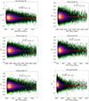 |
Fig. A.1. Results for PSP encounters 1 to 6: Spectral index of the magnetic power αB as a function of the background magnetic field STD. The slope of the red linear fit γ and the values of this fit at the far left and far right of the figure are indicated. All fits have a P-value of P < 0.001. |
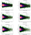 |
Fig. A.2. Results for PSP encounters 7 to 12: Spectral index of the magnetic power αB as a function of the background magnetic field STD. The slope of the red linear fit γ and the values of this fit at the far left and far right of the figure are indicated. All fits have a P-value of P < 0.001. |
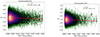 |
Fig. A.3. Results for PSP encounters 13 and 14: Spectral index of the magnetic power αB as a function of the background magnetic field STD. The slope of the red linear fit γ, and the values of this fit at the far left and far right of the figure are indicated. Both fits have a P-value of P < 0.001. |
Appendix B: Spectral index versus background magnetic field STD for distinct intervals of heliocentric distance
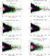 |
Fig. B.1. Results for PSP encounters 1 to 14, split into distinct heliocentric distance intervals. Spectral index of the magnetic power αB as a function of the background magnetic field STD. The slope of the red linear fit γ and the values of this fit at the far left and far right of the figure are indicated. All fits have a P-value of P < 0.001, except for the fit for 60 R⊙ < r, which instead has P < 0.06. |
All Figures
|
Fig. 1. Magnetic spectral indices αB vs. STD of the background magnetic field for the 12th encounter of PSP. |
| In the text | |
|
Fig. 2. Extraction of the measure for the background STD from the data. |
| In the text | |
|
Fig. 3. Slope γ of the decreasing trend in the spectral index with increasing magnetic field STD for encounters 1 up to and including 14. A histogram is added to better visualize the distribution of the γ values in all encounters. |
| In the text | |
|
Fig. 4. Magnetic spectral index αB vs. STD of the background magnetic field for PSP encounters 1–14 for time windows in which the position of the PSP was between 20 and 30 R⊙. |
| In the text | |
|
Fig. 5. Slope of the decreasing trend of the spectral index with increasing magnetic field STD for different distinct intervals of the heliocentric distance. The data taken into consideration consist of PSP encounters 1–14, with 12 days of data per encounter. |
| In the text | |
|
Fig. 6. Three samples of artificial colored noise, mimicking the actual magnetic field data. |
| In the text | |
|
Fig. 7. Variation in the spectral index αB as a function of background STD for the artificial colored noise illustrated in Fig. 6. No downward trend is recovered. |
| In the text | |
|
Fig. 8. Kurtosis of the radial magnetic field component vs. the STD of the total background magnetic field. |
| In the text | |
|
Fig. A.1. Results for PSP encounters 1 to 6: Spectral index of the magnetic power αB as a function of the background magnetic field STD. The slope of the red linear fit γ and the values of this fit at the far left and far right of the figure are indicated. All fits have a P-value of P < 0.001. |
| In the text | |
|
Fig. A.2. Results for PSP encounters 7 to 12: Spectral index of the magnetic power αB as a function of the background magnetic field STD. The slope of the red linear fit γ and the values of this fit at the far left and far right of the figure are indicated. All fits have a P-value of P < 0.001. |
| In the text | |
|
Fig. A.3. Results for PSP encounters 13 and 14: Spectral index of the magnetic power αB as a function of the background magnetic field STD. The slope of the red linear fit γ, and the values of this fit at the far left and far right of the figure are indicated. Both fits have a P-value of P < 0.001. |
| In the text | |
|
Fig. B.1. Results for PSP encounters 1 to 14, split into distinct heliocentric distance intervals. Spectral index of the magnetic power αB as a function of the background magnetic field STD. The slope of the red linear fit γ and the values of this fit at the far left and far right of the figure are indicated. All fits have a P-value of P < 0.001, except for the fit for 60 R⊙ < r, which instead has P < 0.06. |
| In the text | |
Current usage metrics show cumulative count of Article Views (full-text article views including HTML views, PDF and ePub downloads, according to the available data) and Abstracts Views on Vision4Press platform.
Data correspond to usage on the plateform after 2015. The current usage metrics is available 48-96 hours after online publication and is updated daily on week days.
Initial download of the metrics may take a while.