| Issue |
A&A
Volume 677, September 2023
|
|
|---|---|---|
| Article Number | A185 | |
| Number of page(s) | 16 | |
| Section | Astronomical instrumentation | |
| DOI | https://doi.org/10.1051/0004-6361/202346257 | |
| Published online | 27 September 2023 | |
Astrometry in crowded fields towards the Galactic bulge
1
European Southern Observatory,
Karl-Schwarzschild-Straße 2,
85748
Garching, Germany
e-mail: This email address is being protected from spambots. You need JavaScript enabled to view it.
2
Instituto de Astrofísica, Facultad de Ciencias Exactas, Universidad Andrés Bello,
Fernández Concha 700, Las Condes,
Santiago, Chile
3
Vatican Observatory,
00120
Vatican City State, Italy
4
Departamento de Fisica, Universidade Federal de Santa Catarina,
Trinidade
88040-900,
Florianopolis, Brazil
Received:
27
February
2023
Accepted:
19
July
2023
Abstract
Context. The astrometry towards the Galactic bulge is hampered by high stellar crowding and patchy extinction. This effect is particularly severe for optical surveys such as the European Space Agency satellite Gala.
Aims. In this study, we assess the consistency of proper motion measurements between optical (Gaia DR3) and near-infrared (VIRAC2) catalogues in comparison with proper motions measured with the Hubble Space Telescope (HST) observations in several crowded fields towards the Galactic bulge and in Galactic globular clusters.
Methods. Assuming that the proper motion measurements are well characterised, the uncertainty-normalised proper motion differences between pairs of catalogues are expected to follow a normal distribution. A deviation from a normal distribution defines the inflation factor r. By multiplying the proper motion uncertainties with the appropriate inflation factor values, the Gaia (VIRAC2) proper motion measurements are brought into a 1σ agreement with the HST proper motions.
Results. The inflation factor (r) depends on stellar surface density. For the brightest stars in our sample (G < 18), the dependence on G-band magnitude is strong, corresponding to the most precise Gaia DR3 proper motions. We used the number of observed Gaia DR3 sources as a proxy for the stellar surface density. Assuming that the HST proper motion measurements are well determined and free from systematic errors, we find that Gaia DR3 proper motion uncertainties are better characterised, having r < 1.5 in fields with a stellar number density with fewer than 200 Gaia DR3 sources per arcmin2, and are underestimated by up to a factor of 4 in fields with stellar densities higher than 300 sources per arcmin2. For the most crowded fields in VIRAC2, the proper motion uncertainties are underestimated by a factor of 1.1 up to 1.5, with a dependence on J-band magnitude. In all fields, the brighter sources have the higher r value. At the faint end (G > 19), the inflation factor is close to 1, meaning that the proper motions already fully agree with the HST measurements within 1σ.
Conclusions. In the crowded fields common to both catalogues, VIRAC2 proper motions agree with HST proper motions and do not need an inflation factor for their uncertainties. Because of the depth and completeness of VIRAC2 in these fields, it is an ideal complement to Gaia DR3 for proper motion studies towards the Galactic bulge.
Key words: astrometry / proper motions / Galaxy: bulge / Galaxy: kinematics and dynamics
© The Authors 2023
 Open Access article, published by EDP Sciences, under the terms of the Creative Commons Attribution License (https://creativecommons.org/licenses/by/4.0), which permits unrestricted use, distribution, and reproduction in any medium, provided the original work is properly cited.
This article is published in open access under the Subscribe to Open model. This email address is being protected from spambots. You need JavaScript enabled to view it. to support open access publication.
1 Introduction
The Galactic bulge1 is the only inner region of a large galaxy in which individual stars can be resolved from the ground. Therefore, the Galactic bulge provides the possibility of studying stellar interactions in high-density environments on galactic scales. As galaxies form inside-out, studies of the stellar populations in the Galactic bulge provide links to the early formation of the Milky Way (e.g. Barbuy et al. 2018; Zoccali 2019; Fragkoudi et al. 2020). However, the highly variable reddening and stellar crowding mean that characterising this is a difficult task. Many studies thus focused on specific low-reddening windows in the bulge (e.g. Zoccali et al. 2003; Clarkson et al. 2008; Johnson et al. 2011; Bernard et al. 2018) or on areas of particular interest, such as the Galactic centre with its supermassive black hole (Gillessen et al. 2009; GRAVITY Collaboration 2018, 2020) and the nuclear star cluster (e.g. Pfuhl et al. 2011; Schödel et al. 2014; Feldmeier-Krause et al. 2015; Chatzopoulos et al. 2015; Nogueras-Lara et al. 2020). Surveys of the inner Milky Way including the bulge led to global reddening and stellar crowding maps (Gonzalez et al. 2012, 2013; Nidever et al. 2012; Schultheis et al. 2014; Nataf et al. 2016; Surot et al. 2020; Nogueras-Lara et al. 2021; Zhang & Kainulainen 2022; Sanders et al. 2022), from which more detailed and accurate morphology and structural parameters of the bulge could be derived (Wegg & Gerhard 2013; Portail et al. 2017; Simion et al. 2017; Clarke et al. 2019). It is now established that in addition to the thick bar (Stanek et al. 1994; Babusiaux & Gilmore 2005), the Galactic bulge also presents an X-shape (McWilliam & Zoccali 2010; Nataf et al. 2010; Gonzalez et al. 2015; Ness & Lang 2016) in a composite structure that is challenging to unravel because many components overlap (Zoccali & Valenti 2016; Kunder et al. 2016; Lucey et al. 2021; Wylie et al. 2022; Marchetti et al. 2022; Rix et al. 2022).
The different stellar populations in the bulge exhibit different kinematics. Proper motions are thus a valuable tool for distinguishing bulge and disc stars and for identifying structures such as streams or globular clusters (Horta et al. 2021; Kader et al. 2022; Garro et al. 2022). They can also be used to characterise structures such as the nuclear star cluster or the nuclear stellar disc (Clarke & Gerhard 2022; Shahzamanian et al. 2022; Nogueras-Lara 2022).
Recent near-infrared (NIR) surveys have revolutionised our understanding of the Galactic bulge. The Vista Variables in the Via Lactea (VVV) and its extension, the VVV eXtended survey (VVVX), created maps of the Galactic bulge and of the southern part of the disc (−130 deg < l < 20 deg and −15 deg < b < 10 deg), covering ~ 1700 deg2 in five NIR pass-bands: Z(0.87 μm), Y(1.02 μm), J(1.25 μm), H(1.64 μm), and Ks(2.14 μm) (Minniti et al. 2010; Saito et al. 2012; Alonso-García et al. 2018). The VVV observations started in 2010 and continued with VVVX until 2022, collecting many tens of epochs in the Ks band. Some areas in the central parts have >100 epochs, enabling proper motion measurements over a baseline of more than ten years. In the following, we use VVV to denote observations within the central bulge area that were collected within the original VVV survey as well as its extension VVVX.
VIRAC2 (Smith et al., in prep.) is the second data release of the VVV Infrared Astrometric Catalogue (VIRAC; Smith et al. 2018). VIRAC2 is 90% complete up to Ks ~ 16 across the VVV bulge area (Sanders et al. 2022). Its proper motions are anchored to the Gaia absolute reference frame.
In addition to the NIR surveys, Gaia presents an impressive amount of data that are a valuable source for studies of all Galactic components. The third data release (DR3) of the Gaia survey (Gaia Collaboration 2022) includes the astro-metric and photometric data for ~1.5 billion sources spanning 34 months of observations (Gaia Collaboration 2021). Gaia DR3 astrometry is given in the International Celestial Reference System (ICRS) with the 2016.0 reference epoch. However, the survey has a completeness below 60% for sources at G ~ 19 or fainter, and the completeness in stellar densities is about 5 × 10⁵ stars deg−2, which happens in crowded fields such as those within globular clusters. The completeness of Gaia DR3 is below 20% even for brighter sources in fields with stellar densities of about 106–107 stars deg−2, which also includes the Galactic bulge (Fabricius et al. 2021; Everall & Boubert 2022; Cantat-Gaudin et al. 2023).
As for any type of measurement, the Gaia data are subject to systematics coming from the instrument itself or from the data processing. The systematics affect both photometry and astrometry. The systematic offset in parallax or proper motion (i.e. zero-points) can be obtained by a comparison with sources whose parallax and proper motion are known, such as quasars or binaries. The zero-point can depend on magnitude, colour, and position (see Lindegren et al. 2021a; Riello et al. 2021). The systematics could lead to an over- or underestimation of measurements and their uncertainties.
The underestimation of the uncertainty estimates for positions, parallaxes, and proper motions (i.e. the astrometric solution) is a known caveat since Gaia DR1, where a formula for an inflation factor for the parallax formal uncertainties is provided (Lindegren et al. 2016). The underestimate of astrometric uncertainties of sources in crowded regions has been presented by Arenou et al. (2018). For Gaia DR2, the formula for the parallax uncertainty underestimation factor includes both the systematics and the formal (catalogue) uncertainties (Lindegren et al. 2018). In DR2, the underestimation factor for the parallax is between 2 and 3 for most sources. While DR3 improves this, the parallax formal uncertainties are underestimated for faint stars and stars in crowded fields (see Fabricius et al. 2021); these stars might also present a larger underestimation in their proper motion uncertainties.
Several studies have investigated the accuracy of Gaia proper motion and parallax measurements, which led to correction factors (e.g. Fabricius et al. 2021; El-Badry et al. 2021; Vasiliev & Baumgardt 2021; Maiz Apellániz et al. 2021; Babusiaux et al. 2023). Here we provide an independent study that has been triggered by our search for hypervelocity stars in the inner bulge (Luna et al. 2019). Hypervelocity stars are objects that are unbound from the Galactic potential, and they are extremely rare. We wish to identify outliers in a large distribution. Therefore, it is particularly important to know how reliable the measurements and their errors are. In this study, we aim to validate the use of Gaia DR3 and VVV astrometry in crowded fields by comparing them to different sets of accurate and precise proper motions of HST observations.
2 Cross match of the data sets and catalogues
The measurements of the stellar positions based on the HST photometry are very precise. The ACS/WFC plate scale of 50 mas pixel−1 can result in proper motion measurements as accurate as 0.3 mas yr−1 with observations spanning a baseline of two years (Clarkson et al. 2008). The plate scale of WFC3 UVIS channel is 40 mas pixel−1 , enabling similar precision for proper motion measurements (Brown et al. 2009). With a more extended observing baseline of more than nine years, Calamida et al. (2014) reported a proper motion measurements accuracy of about 0.1 mas yr−1 for stars as faint as F606W ~ 25.5 mag, for which they combined data from both cameras. For comparison, the typical precision2 of Gaia DR3 proper motions is 0.1 mas yr−1 at G = 18 and 0.5 mas yr−1 at G = 20. Gaia DR3 proper motions are superior for brighter stars, but these proper motions are close to the saturation of the WFC/ACS detector in the HST data sets that cover the dense bulge fields with multi-epoch observations. A more detailed comparison between the two instruments is given in del Pino et al. (2022) and Massari et al. (2020).
As a benchmark, we used the WFC3 Galactic bulge Treasury Program: Populations, Formation History, and Planets (BTP)3 (Clarkson et al. 2008; Brown et al. 2009, GO-11664; PI: Brown, T. M.), which consists of observations of four low-reddening windows that map different environments in the Galactic bulge: the SWEEPS, Stanek, Baade, and Ogle29 windows (see Table 1 for their location and extinction). The BTP was created to study resolved stellar populations using the WFC3 on the HST. The BTP provides a deep astrometric and photometric catalogue, reaching F606W~ 26, which is several magnitudes below the main-sequence turn-off (MSTO), around F606W~ 20. The stars included in the BTP are field stars because there are no stellar clusters in these fields of view (FoV).
To cross-match the HST sources with Gaia DR3 and then compare their proper motions, we first transformed the BTP proper motions, which are provided in the catalogue in units of pixel per baseline, into proper motions components along RA and DEC using a 30 mas pixel-1 scale, as reported in the BTP catalogue description4 (Brown et al. 2009). We note that the images and proper motions are oriented north-east. The baseline for the SWEEPS window is 6.2 yr, with observations from 2004 to 2010, while for the Stanek, Baade, and Ogle29 windows, the baseline is two years, with observations from 2010 to 2012. The longer baseline for the SWEEPS window is possible through a previously observed programme in addition to the BTP (Sahu et al. 2006; Clarkson et al. 2008).
After we computed the proper motions in masyr−1, we cleaned the data set by examining the quality flags in the catalogues. The BTP positions and proper motions come from a point spread function fit that uses three different photometric methods, depending on the brightness of the source. Within the BTP catalogue, the parameter qual indicates the fit quality and ranges between 0 and 1. We selected the sources with the best quality fit, hence the best-characterised photometry and astrometry, restricting 0.9 ≤qual≤ 1. This selection excludes bright sources close to the saturation of the WCF/ACS detector.
Following Battaglia et al. (2022)5, we selected sources for Gaia DR3 with a complete astrometric solution (astrometric_params_solved ≥ 31) that were not flagged as a duplicated source, and having a renormalised unit weight error (RUWE) < 1.4 (Lindegren et al. 2018). The RUWE is an indicator of the quality of the astrometric fit. This threshold was set to select single sources with good astrometric measurements. In crowded fields, RUWE values may be underestimated. In principle, the requirement of RUWE < 1 .4 might therefore be relaxed and the statistics thus increased.
The positions of stars in the BTP catalogue, given in equatorial coordinates (J2000 epoch), were propagated to 2016.0, the Gaia DR3 reference epoch. We performed an initial cross match within 0.″5 tolerance in position using the astropy package SkyCoord.match_to_catalog_sky, which uses a KD-tree to find the nearest neighbour. The HST astrometric reference frame is offset ≤0.″3 with respect to Gaia DR1 (Clarkson et al. 2018) in each coordinate, and a similar offset may still be present in Gaia DR3 (Kozhurina-Platais & Martlin 2021). To take systematic effects into account, we searched for trends between the proper motions and other parameters such as Gaia DR3 colours, magnitude, or position (e.g. Massari et al. 2020, 2018). There is no clear trend with any of the parameters, however.
Then, the cross match was refined by comparing the source G-band magnitude and the HST F555W (or F606W) magnitude, excluding in this way the spurious matches. Figure 1 shows the magnitude difference for the SWEEPS window. The correct matches lie below the red line. The cross match was made individually in the different studied fields, and the separation distribution of cross-matched sources in each field was centred at ~0.″2 with a standard deviation of 0.″4.
Throughout the text, the comparison between Gaia DR3 and the BTP windows is illustrated using the BTP-SWEEPS window with its corresponding figures. The same method was applied for all BTP windows, and their figures can be found in Appendix A. In the case of Baade’s window, there are 371 cross-matched sources within 0.″5, but most of them are spurious matches, with a large G-band and F555W magnitude difference. Because the final sample of well-matched sources in Baade’s window consists of only 30 sources, we do not consider this field in the rest of this work.
Although the main HST data sets have 104–105 sources, with 103 Gaia DR3 sources in the same FoV, the final data set after the cross match has only a few 102 sources per field. Figure 2 illustrates the decrease in the number of sources when the different quality cuts and cross-match refinements were applied. From top to bottom of Fig. 2, sources from Gaia DR3 catalogue are plotted in the right panels, and sources in the HST-BTP-SWEEPS window are plotted in the left panel. The panels in the second row show the sources after the quality cuts described in the previous paragraphs. The final two panels show the cross-matched sources within 0.″5 of the tolerance in position (grey), and in the bottom panel, the final sample used for the study (orange). The orange points correspond to the orange points in Fig. 1. The number of sources remaining in each step of this cross-matching procedure for the HST-BTP-SWEEPS field is shown above each panel in Fig. 2.
The low number of final cross-matched sources is largely a consequence of the different survey depths. While HST reaches magnitudes well below F606W = 24 and mostly detects the main-sequence stars, Gaia is limited to stars brighter than G = 20 mag. In the bright end, Gaia is more complete, but HST begins to saturate, with its bright detection limit around F606W= 18 mag. This is illustrated in Fig. 3, showing the colour-magnitude diagrams (CMDs) of Gaia DR3 and HST in the SWEEPS field.
In addition to the comparison of the HST and Gaia proper motions in high-density fields in the bulge using the BTP catalogue, we also compared the HST and Gaia DR3 proper motions in three fields in the outskirts of ω Cen (GO-14118 and GO-14662; PI: Bedin, L. R. catalogues: Bellini et al. 2018; Scalco et al. 2021; Libralato et al. 2018) and in NGC 6652 (GO-13297; PI: Piotto, G. Catalogue: Libralato et al. 2022), a globular cluster in Baade’s window.
Finally, we also validated the proper motion uncertainties of the VIRAC2 catalogue with respect to the HST proper motions in three bulge fields: the SWEEPS, Stanek, and Ogle29 windows. The comparison was made for the J band in VIRAC2 and F110W in HST. The data sets were cross-matched and cleaned, for which we adopted the same quality flags as described above for Gaia . As a quality cut in VIRAC2, we selected sources with a complete (five-parameter) astrometric solution, non-duplicates, and sources that were detected in at least 20% of the epochs. As an additional quality parameter, we selected sources with a unit weight error uwe< 1.2, which is a threshold to select single sources with good astrometric measurements (L. C. Smith, priv. comm.). The rest of the cross match was made following a procedure similar to that described for the Gaia-BTP comparison. The cross-matched sources have a mean separation of 0.″25. From the VIRAC2 initial sample of 5199, 5623, and 3856 in the SWEEPS, Stanek, and Ogle29 windows, the final sample used for the comparison resulted in 557 sources in the SWEEPS field, 1515 sources in the Stanek field, and 171 in the Ogle29 field. The larger number statistics in the SWEEPS and Stanek fields are a result of the better matching magnitude range between the VVV and Gaia DR3. The H – J versus J CMDs of the initial and final data sets are given in Appendix B.
Galactic coordinates, extinction coefficient, and the final number of matched sources (Nf) used for the analysis of the four BTP low-reddening windows; the outskirt fields of ωCen, F1, F2, and F3; and the globular cluster NGC 6652.
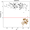 |
Fig. 1 Gaia DR3 G-band and HST F555W magnitude difference. The initial position cross match is refined with a selection of stars that have similar magnitudes. The good matches are below the solid red line at F555W − G = 1. |
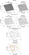 |
Fig. 2 Number of sources in Gaia DR3 and HST-BTP in the SWEEPS field. From top to bottom: Initial sample in the same FoV after applying the quality cuts described in Sect. 2, after a cross match between the data sets with a tolerance of 0.″5, and the final sample used for the study. The position of the sources in the final sample is plotted in orange. In the second row, the lack of sources in the corners of the BTP data set arises because they did not have a proper motion value in the BTP catalogue. This is due to small differences in the field orientation between different epoch exposures. |
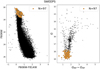 |
Fig. 3 Colour-magnitude diagrams of Gaia DR3 and HST in the SWEEPS window. The orange points correspond to the location of the cross-matched sources after the quality cuts and a 3σ clipping in the uncertainty normalised proper motion difference. The black dots are the total sources in the field after the quality cuts. The two catalogues overlap in a short magnitude range. |
3 Inflation factor
When we assume the proper motions in two different uncorrelated catalogues μ1 and μ2 with their corresponding uncertainties σ1 and σ2, and when they follow a Gaussian distribution, their uncertainty-normalised difference ( ) should follow a normal distribution. If the proper motion and/or its uncertainties in one of the catalogues are under- or overestimated, the true proper motion uncertainty would be
 (1)
(1)
with r being the inflation factor needed to bring μ1 into a 1σ agreement with μ2.
Then, the variance of the uncertainty-normalised proper motion difference is
 (2)
(2)
Thus
 (3)
(3)
where r is the individual inflation factor for each star in the sample, which depends on the individual uncertainties σ1 and σ2, and the standard deviation K of the uncertainty normalised proper motion difference of the parent population.
We took μ1 and σ1 as the reported Gaia measurements and μ2 and σ2 as the HST measurements, where we assumed that the HST proper motion measurements are true values with well-determined uncertainties that are neither under- nor overestimated. Because we know that this is not the case for the BTP catalogue, we looked for systematics in the HST data, as discussed for example in Bellini et al. (2011) and Libralato et al. (2022), but found none. For globular clusters, we used HST proper motions that were corrected for HST systematics (see Sect. 4.3 and 4.4).
In this way, we incorporated the proper motion uncertainty underestimation completely into Gaia DR3, even though HST proper motions are not free of systematics. Our goal was to set an upper limit on the true underestimation of the Gaia DR3 proper motion uncertainties. To complement this, we include in Appendix D an analysis of the change in the inflation factor when systematics in addition to the HST proper motions are introduced. We show that for the SWEEPS window, r varies by 20% within the sampled range, but for the Stanek and Ogle29 windows, r decreases up to 50% with larger PM uncertainty. The inflation factor was derived independently for the proper motion components in RA and Dec. Therefore, the correlation parameter between the RA and Dec components in Gaia DR3 does not influence the analysis.
Any systematic errors in Gaia values must be subtracted from the reported formal uncertainties to obtain the true uncertainties. When the systematic errors σ2 are accounted for, the true Gaia uncertainties would be
 (4)
(4)
Lindegren et al. (2021b) derived Gaia DR3 parallax and proper motion systematics through the angular covariance functions V(θ), which describe the spatial correlation of errors in astrometric quantities and which depend on the angular separation in degree of two sources. The authors estimated the systematics from a quasar sample and found V(θ)μ ~ 550 μas2 yr−2, which is in the short-separation limit (0° < θ < 0.125°). This corresponds to a systematic error of σS = 0.017 mas yr−1. Vasiliev & Baumgardt (2021) extended this analysis for shorter separations with stars in Galactic globular clusters and reported V(θ)μ ~ 700 μas2 yr−2 in the short-separation limit. This corresponds to a systematic error of σS = 0.026 mas yr−1. These numbers indicate the maximum precision of the proper motion measurements. This is an improvement with respect to DR2, where the systematic was constrained to 0.066 mas yr−1 for sources with G > 16 in Gaia DR2 (Lindegren et al. 2018). The value of σ2 can otherwise be obtained as the zero-point of the proper motion of quasars or other absolute proper motion reference frame tracers, which we lack in this comparison. Hence, our approach can only constrain the inflation factor r, which absorbs part of the systematic errors.
Taking σ2 into account, the individual inflation factor is given by
 (5)
(5)
where σ2 = 0.026 mas yr−1 because the data set areas are within the short-separation limit.
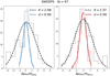 |
Fig. 4 Normalised proper motion difference distribution for the SWEEPS field. The dashed curves are the initial distributions in each coordinate component. The solid curves are the distributions after Gaia DR3 proper motion uncertainties are multiplied by the inflation factor r. The standard deviation of the distribution before and after applying the inflation factor is labelled Κ and σ, respectively. |
4 Results of the fit
In this section, we present the procedure and results of a Gaussian mixture model (GMM) fit to the uncertainty-normalised proper motion difference. The same GMM fitting procedure that was applied to the BTP data set was then also applied to assess the consistency of the proper motion for other data sets with respect to Gaia DR3.
4.1 BTP
Due to the lack of sources in the bulge that can be used to transform the proper motions into an absolute reference frame, the proper motions of the BTP fields are relative to the median of a sample of bulge stars in the MSTO and fainter (Clarkson et al. 2018). We transformed the proper motions into absolute proper motions anchored to Gaia by subtracting the mean of the μBTP – μGaia DR3 proper motion distributions. The BTP catalogue does not provide individual proper motion uncertainties, but an upper limit of 0.3 mas yr−1, which we assumed as the uncertainty value for the cross-matched sources. To assess the impact of this assumption on the results of our study, we explored the extended SWEEPS catalogue (Calamida et al. 2014), which contains individual proper motion uncertainties for all measured sources. The results from the analysis of the extended SWEEPS catalogue are consistent with those of the SWEEPS-BTP window. This is further discussed in Sect. 4.2, and the corresponding plots are provided in Appendix E.
We compared the uncertainty normalised distributions of proper motion differences separately in RA and Dec and fit them with a Gaussian (see Fig. 4), keeping only the stars within 3σ of the distribution in each coordinate. With K being the standard deviation of Δμ/σμ, we applied Eq. (3) independently in each coordinate to obtain the individual inflation factor r of each source, which was to be multiplied by its Gaia proper motion uncertainty.
In Fig. 4 we show Δμ/σμ in RA (left panel) and Dec (right panel) for the 97 sources in the final sample in the BTP-SWEEPS window. The standard deviations of the Δμ/σμ distribution before and after applying the inflation factor are labelled K and σ, respectively. The value was 2.98 in RA and 2.57 in Dec, and after applying the median inflation factor, this reached ~ 1 in both cases. The dashed Gaussian corresponds to the initial Δμ/σμ distribution, and the solid-coloured Gaussian corresponds to the distribution after the inflation of the Gaia DR3 proper motion uncertainty. The equivalent of Fig. 4 for the studied fields is provided in Appendix C.
The standard deviation of the distribution after the inflation of the Gaia DR3 uncertainties is not exactly one because we used the median value of r instead of an individual value for each star. The inflation factor r depends strongly on the magnitude, as shown in Fig. 5. This is further described in Sect. 5.
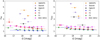 |
Fig. 5 Dependence of the inflation factor r on the G-band magnitude of the studied HST fields. The points represent the medians of the magnitude bins, and for r, the error bars are the 16th and 84th percentiles. The bars in G indicate the magnitude distribution in a given bin, where the marker is the median. The plotted data are listed in Table 2. |
4.2 Extended SWEEPS catalogue
Calamida et al. (2014) published the extended baseline of observations of the SWEEPS window covering nine years (GO-9750 and GO-12586; PI: Sahu, K.C.) and derived proper motions in Galactic coordinates with precision around 0.1 mas yr−1 at F606W = 25.5 mag and around 0.5 mas yr−1 at F606W = 28 mag. Based on these proper motions, they revealed the white dwarf cooling sequence in the Galactic bulge. We analysed this data set as well because it offers an independent validation of the results based on the BTP data by extending observations of the same field (SWEEPS) over a longer baseline and presenting individual uncertainties for all sources in the HST data set, rather than an average upper limit.
To compute the inflation factor and compare it with the results for the BTP windows, we transformed the proper motions and their uncertainties from Galactic coordinates into equatorial coordinates, assuming that the proper motions are not correlated. The catalogue includes no correlation coefficient.
The median inflation factor for the full-SWEEPS is consistent with the median inflation factor of the BTP-SWEEPS for every magnitude bin except for G < 18.5 (see Appendix E). This bright end of the magnitude overlap between Gaia DR3 and HST includes only a few sources. Because the full-SWEEPS catalogue lacks quality flags, it is possible that a few unreliable astrometric measurements affect the sources in the bright bin.
4.3 ω Cen
The outer fields of ω Cen (F1, F2, and F3) have a lower density than the BTP windows. In this case, the value of r is closer to one (Fig. 5). This indicates that the uncertainties of the Gaia DR3 proper motions are mostly consistent with those from the HST catalogues. This shows that our procedure is consistent with previous findings such as Maíz Apellániz et al. (2021), Vasiliev & Baumgardt (2021), and Babusiaux et al. (2023).
We tried to analyse the core of ω Cen with the HST data provided in Bellini et al. (2017). However, the severe crowding in its core prevents any well-behaved measurement with Gaia. The majority of the Gaia DR3 sources in this region have a RUWE > 1.4 and were thus rejected based on the quality cuts.
4.4 NGC6652
Recently, Libralato et al. (2022) published a homogeneous photometric and astrometric catalogue of 56 globular clusters in the Gaiaxy. One of them is NGC 6652, a globular cluster of particular interest for this study because it is located within Baade’s window in the bulge, and because its data have been processed following the same procedure as the outer ω Cen fields. The inflation factor is larger than the one derived for the ω Cen out-skirt fields, but lower than the bulge fields, indicating that their proper motions are better characterised than those of the BTP fields (Fig. 5).
Comparisons with the HST globular cluster were also used to validate Gaia DR2 astrometry (Arenou et al. 2018) and DR3 (Fabricius et al. 2021). The normalised dispersion of the differences in ω Cen is close to one, indicating that the uncertainties are correctly estimated (Arenou et al. 2018).
4.5 VIRAC2
As VIRAC2 covers the inner part of the bulge, we have data for three of the seven studied fields: the SWEEPS, Stanek, and Ogle29 windows. VIRAC2 proper motions are given in equatorial coordinates and are anchored to the Gaia DR3 absolute reference frame. Hence, we transformed the HST-BTP proper motions into absolute proper motions in the same manner as before by subtracting the mean of the μΒΤΡ – μVIRAC2 proper motion distributions independently in RA and Dec. For the BTP uncertainties, we assumed an upper limit of 0.3 mas yr−1. Figure 6 is equivalent to Fig. 4, where the original Δμ/σμ in each coordinate are plotted as dashed Gaussians, and the solid Gaussians are the distributions after the inflation of the VIRAC2 proper motion uncertainties. The top panels correspond to the comparison of VIRCAC2 versus HST in the BTP-SWEEPS field, the middle panels compare VIRAC2 and BTP-Stanek, and the bottom panels correspond to the comparison with the BTP-Ogle29 field.
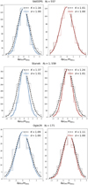 |
Fig. 6 Normalised proper motion difference distribution for VIRAC2 vs. SWEEPS-BTP (top), VIRAC2 vs. Stanek-BTP (middle), and VIRAC2 vs. Ogle29-BTP (bottom). The dashed curves are the initial distributions in each coordinate component. The solid curves are the distributions after the VIRAC2 uncertainties are multiplied by the inflation factor r. |
Median inflation factor (r) in a given G-band magnitude range for the seven studied fields.
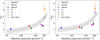 |
Fig. 7 Dependence of the inflation factor r on the number density defined for sources found in the Gaia DR3 catalogue in a given field. The median r for the different fields is plotted with different colours. The error bars correspond to the 16th and 84th percentile in the distribution of r across the magnitude range of a given field. The shade is the 1σ uncertainty on the fit. The plotted data are listed in Table 3. |
Number of sources in Gaia DR3 in a given field, area of the field, and median values of the inflation factor r.
5 Analysis and discussion
In the catalogue validation of Gaia DR3, Fabricius et al. (2021) found an offset in the unit weight error of the parallax with respect to their uncertainty. The offset for the bulk of the sources is 1.05 for a five-parameter (positions, parallax, and proper motions) astrometric solution and 1.22 for a six-parameter astrometric solution, where the sixth parameter is the pseudo-colour, which is the astrometrically estimated effective wave number when the source colour GBP – GRP was not available. Sources with a six-parameter solution show more systematics and spurious solutions (Lindegren et al. 2021a; Fabricius et al. 2021). An additional underestimation factor depends on the G-band magnitude (Figs. 20 and 21 in Fabricius et al. 2021).
del Pino et al. (2022) applied the offsets (1.05 or 1.22) derived specifically for parallax uncertainties as underestimation factors also to correct for the uncertainties for all astro-metric parameters (positions, parallax, and proper motions) in GaiaHUB. This code uses HST observations as an additional epoch for Gaia. They showed that this resulted in an improved proper motion accuracy for the case studies.
This is not the only case in which an inflation factor to correct for the underestimation of Gaia uncertainties has been derived for different cases with success. El-Badry et al. (2021) found that Gaia DR3 parallax uncertainties are underestimated up to 50% by comparing the parallax of binary components in a catalogue they constructed assuming that the pairs are bound. Maíz Apellániz et al. (2021) derived inflation factors for the parallax in globular clusters by forcing the parallax distribution to be normal. The inflation factor is larger for stars in the magnitude range of 12 < G < 18. They reported similar values as Fabricius et al. (2021). Following the same procedure, Babusiaux et al. (2023) derived an inflation factor for the radial velocity uncertainty in a sample of open clusters. They fit a two-order polynomial to the factor as a function of magnitude (GRVS) and effective temperature and in this way, provided a formula for the uncertainties inflation.
Furthermore, the astrometric solution of a source may not be reliable depending on its position. Rybizki et al. (2022) developed a classifier for accurate astrometric solutions in Gaia DR3 and reported that the majority of sources in the direction of the bulge have a spurious astrometric solution. They compared Gaia DR3 proper motions with OGLE IV proper motions and found that the uncertainties are underestimated for either one or both of them. The scanning law could amplify the disturbance of a close neighbour, which would have a larger effect in a crowded field such as the bulge. This in turn would result in spurious astrometric solutions.
As a result of selecting the sources with the best quality and the difference in crowding of the studied fields, the final sample of our data sets covers different magnitude ranges, as shown in Fig. 5. For the different studied fields, Table 2 lists the median inflation factor and the number of sources (N) we use to compute it in a given bin. The number of sources in each magnitude bin ranges between ~20 in the brightest magnitude bins and >100 at G < 18 for some fields, such as the ω Cen fields. To verify whether the low number statistics and the individual sources with outlying r may affect the median value of r, we performed a bootstrap sampling.
To account for the influence of the low number statistics in the results and to estimate the uncertainty of the inflation factor derivation, we performed a bootstrap sampling with 1000 iterations of N – 5 elements, where N is the number of sources in the parent sample. The error bars for r in Fig. 5 are smaller than the marker in most cases.
Figure 7 shows the dependence of r on stellar surface density, where the proxy for the density is the number of Gaia DR3 sources per arcmin2 in a given field (N), that is, before any quality cut and for the entire magnitude range. Gaia uncertainties are more strongly underestimated as the stellar surface density increases, such as for the SWEEPS and Stanek fields. This dependence follows the relation
 (6)
(6)
where i = RA, Dec; and α = −0.46 ± 0.38 in RA and α = −0.27 ± 0.38 in Dec.
The dependence of the inflation factor on density has a trend that follows Eq. (6). This trend is plotted as a dashed grey line in Fig. 7. Vasiliev & Baumgardt (2021) studied the dependence of the parallax uncertainty inflation factor on the stellar density of several Galactic globular clusters. They reported that the parallax inflation factor follows an exponential function that depends on the stellar number density (see their Fig. 5). Although there is a similarity between the shape of their relation and ours, it is not directly comparable because our approach, in contrast to Vasiliev & Baumgardt (2021), compares Gaia to other catalogues. It might be expected that NGC 6652, as a globular cluster in the Galactic bulge, has a higher stellar density than the Ogle29 field. However, the blending that affects Gaia may result in a lower count of sources and hence cause the similar location of both fields in Fig. 7.
The difference between the inflation factor in RA and Dec can be explained as a result of the Gaia scanning law (Gaia Collaboration 2021) because the survey is more precise perpendicular to the ecliptic where the satellite has more transits. We note that the Ogle29 field presents the largest difference between the inflation factor values for RA and Dec when compared to other BTP windows. In this location, the Dec component is oriented close to being perpendicular to the ecliptic and is therefore more precise. The median is 0.25 mas yr−1, while the median σRA is 0.46 mas yr−1.
The inflation factor r shows a strong dependence on magnitude. As the precision in Gaia DR3 increases for brighter sources, a larger r is needed to bring the uncertainty-weighted proper motions into a 1σ agreement with the HST measurements. Figure 5 shows the behaviour of the median inflation factor versus G-band magnitude: The median inflation factor increases towards the bright end. The higher-density fields have overall higher inflation factor values, but the trend with magnitude is similar between the fields.
Although in general, the inflation factor r ranges between 1–2 in the lower-density fields F1, F2, and F3 in ω Cen and in NGC 6652 (see Fig. 5), its value increases in the bright bin (G < 17) in ω Cen F2 field on RA. The reason is the low number of stars (18) in that magnitude bin, which is reflected by the larger error bar for r.
As Gaia DR3 measurements become more precise and HST starts to reach the saturation point, the bright sources whose proper motions diverge from the HST need a larger multiplicative factor to bring them into concordance. Figure 8 shows that from the functional form of Eq. (3), r steeply increases for sources with σGaia < σHST. The vertical line in Fig. 8 represents the point when σGaia = σHST. At the faint end (G > 17), where σGaia > σHST, the photon noise dominates the uncertainties on the systematics (Fabricius et al. 2021). Therefore, the inflation factor has an asymptotic behaviour that tends to the standard deviation (K) of the parent population.
Comparison of VIRAC2 and HST. The precision of the VIRAC2 proper motions is comparable to that of the HST. Table 4 lists the median inflation factor at a given J-band magnitude bin shown in Fig. 9. Figure 9 presents the dependence of the inflation factor r as a function of J-band magnitude for the comparison of VIRAC2 with respect to the HST data in the SWEEPS, Stanek, and Ogle29 BTP fields. In contrast with the results for the inflation factor for the Gaia DR3 proper motion uncertainties (Fig. 7), the comparison with the Stanek window results in a larger inflation factor than for the SWEEPS window. Furthermore, within the range of magnitudes that can be probed, r is nearly constant and does not depend on the brightness. In RA, the VIRAC2 proper motion uncertainties in both fields are slightly underestimated, while the inflation factor in Dec is low, that is, close to one. This analysis shows that the proper motions uncertainties of VIRAC2 and HST are consistent within 1σ.
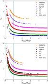 |
Fig. 8 Dependence of the inflation factor on the Gaia and HST uncertainty ratio. The vertical line marks σGaia = σΗSΤ. For sources with σGaia > σΗSΤ, the inflation factor asymptotically reaches a minimum value that corresponds to the standard deviation K of the parent population. This behaviour follows the functional form of Eq. (3). |
Median inflation factor (r) in a given J-band magnitude range for the seven studied fields.
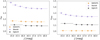 |
Fig. 9 Dependence of the inflation factor r on VIRAC2 J magnitude. The proper motion comparison was made between VIRAC2 and the HST-BTP SWEEPS, Stanek, and Ogle29 windows. The points are the median values of J in each magnitude bin, and the error bars indicate the magnitude distribution at a given bin. In r, the error bars are the 16th and 84th percentile. |
6 Conclusions
We presented an analysis of Gaia DR3 and VIRAC2 proper motion uncertainties in comparison with the HST proper motions in seven fields that present different levels of crowding. Three fields are located in the direction towards the Galactic bulge: the SWEEPS, Stanek and Ogle29 BTP windows. Furthermore, we included three outskirt fields in the globular cluster ω Cen, and the globular cluster NGC 6652. Our main findings concerning the comparison between Gaia DR3 and HST data sets are summarised below.
To bring the Gaia DR3 proper motions into a 1σ agreement with those from the HST, we need an inflation factor to account for the underestimation of their uncertainties and the systematic errors. HST proper motions are not free of systematics, and part of the underestimation may well belong to them. At the moment, we cannot quantify this underestimation in HST proper motions. We therefore imposed the underestimation to Gaia as a way to extend its capabilities and take the inflation as an upper limit on the true underestimation.
The inflation factor dependends on stellar surface density, as indicated by the number of sources in Gaia DR3 catalogue per arcmin2. The dense BTP fields also strongly depend on G-band magnitude, which is driven entirely by the sources for which Gaia DR3 is more precise than HST. These are the brightest sources in the samples.
The dependence of the inflation factor on stellar surface density follows an exponential function with a factor of −0.46 in RA and −0.27 in Dec (see Eq. (6)).
In the most crowded fields, such as the BTP windows, the inflation factor ranges from a factor of two for G ~ 19 to a factor of five at G < 18. In less dense fields, such as the outskirts of the globular clusters ω Cen and NGC 6652, the inflation factor is lower than two, indicating a better agreement of the measurements and their uncertainties.
The large inflation factor in the dense bulge fields implies that the proper motion uncertainties for the brightest sources are underestimated either for the HST or for Gaia DR3, while the proper motion measurements for the globular cluster fields agree much better between the HST and Gaia DR3 catalogues. We note that all of the sources in the final sample of the BTP-Gaia DR3 cross-match have a six-parameter astrometric solution, whereas for the ω Cen outskirt fields F1, F2, and F3, the percentage of six-parameter sources is 38,59, and 60%, respectively. For the globular cluster NGC 6652, it is 62%. This then supports the conclusion that the underestimation of the proper motion uncertainties more likely affects Gaia than the HST measurements in the bulge fields.
VIRAC2 is deeper and more complete than Gaia DR3 in the BTP fields. There is no need for an inflation factor because the VIRAC2 proper motion uncertainties agree well with those of the HST. For these crowded bulge fields, we therefore recommend using VIRAC2 proper motions as a complement of Gaia DR3 proper motions either to increase the statistics or in the case that the astrometric solution for the Gaia DR3 proper motions is poorly behaved.
The main limitation of this study was the low number statistics due to the different depths of the fields. The quality of the measurements appears to be insufficiently characterised in the overlapped magnitude ranges. While we acknowledge the advantage of the NIR data for the highly extincted and crowded Galactic bulge fields, Gaia data are nevertheless very valuable. They provide an independent check on the proper motion measurements, potentially extend the baseline and magnitude range, and provide the possibility of studying outliers in the proper motion distribution and thus of searching for hypervelocity stars, which was our original goal that motivated this study. Gaia proper motion uncertainties will improve as the observational time baseline increases. An improvement of a factor of ~2 can be expected in future releases6. This will allow us to further characterise Gaia versus VIRAC2 astrometric uncertainties and exploit the full capabilities of both surveys.
Acknowledgements
We are grateful to Anthony G. A. Brown for discussing and commenting on the early draft, and Leigh Smith for generously sharing the preliminary VIRAC2 data. A.L. acknowledges support from the ANID Doctorado Nacional 2021 scholarship 21211520, and the ESO studentship. A.L. is grateful to T. Kolcu, Z. Penoyre, S. Verberne, F. A. Evans, E. M. Rossi, and J. de Bruyne for the useful discussions. D.M. gratefully acknowledges support by the ANID BASAL projects ACE210002 and FB210003, by Fondecyt Project No. 1220724, and by CNPq/Brazil through project350104/2022-0. This work has made use of data from the European Space Agency (ESA) mission Gaia (https://www.cosmos.esa.int/gaia), processed by the Gaia Data Processing and Analysis Consortium (DPAC, https://www.cosmos.esa.int/web/gaia/dpac/consortium). Funding for the DPAC has been provided by national institutions, in particular the institutions participating in the Gaia Multilateral Agreement. The data used here may be obtained from https://archive.stsci.edu/prepds/wfc3bulge/. This research made use of Astropy, a community-developed core Python package for Astronomy (Astropy Collaboration 2018, 2013). This research made use of NumPy (Harris et al. 2020), SciPy (Virtanen et al. 2020) and Scikit-learn (Pedregosa et al. 2011). Finally, we are grateful to the anonymous referee for the insightful evaluation of our work and useful suggestions.
Appendix A Color-magnitude diagrams of the studied fields
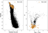 |
Fig. A.1 Colour-magnitude diagrams of Gaia and HST in the Stanek window. The orange points correspond to the location of the cross match after the quality cuts and 3σ clipping. |
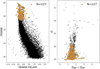 |
Fig. A.2 Colour-magnitude diagrams of Gaia and HST in the Ogle29 window. The orange points correspond to the location of the cross match after the quality cuts and 3σ clipping. |
In this section, we show the HST and Gaia DR3 CMDs for the remaining fields analysed in this study: the BTP-Stanek window, the BTP-Ogle29 window, ω Cen F1, ω Cen F2, ω Cen F3, and NGC 6652. The black points are all the sources in a given field after the quality cuts described in Sect. 2, and the orange points are the final cross-matched sources we used for the study. The figures are the equivalent to Fig. 3, where the left and right panels correspond to the CMD in HST and Gaia DR3 filters, respectively. In addition, we also show the CMD for the Baade’s window BTP catalogue in comparison with Gaia. This field was not used for the analysis because it contains too few cross-matched sources.
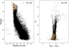 |
Fig. A.3 Colour-magnitude diagrams of Gaia and HST in the Baade window. The orange points correspond to the location of the cross match after the quality cuts and 3σ clipping. |
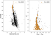 |
Fig. A.4 Colour-magnitude diagrams of Gaia and HST in the ω Cen F1 field. The orange points correspond to the location of the cross match after the quality cuts and 3σ clipping. |
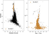 |
Fig. A.5 Colou-magnitude diagrams of Gaia and HST in the ω Cen F2 field. The orange points correspond to the location of the cross match after the quality cuts and 3σ clipping. |
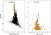 |
Fig. A.6 Colour-magnitude diagrams of Gaia and HST in the ω Cen F3 field. The orange points correspond to the location of the cross match after the quality cuts and 3σ clipping. |
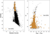 |
Fig. A.7 Colour-magnitude diagrams of Gaia and HST in the globular cluster NGC 6652. The orange points correspond to the location of the cross match after the quality cuts and 3σ clipping. |
Appendix B Color-magnitude diagrams of the studied fields with VIRAC2
In this section, we show the HST and VIRAC2 CMDs for the BTP SWEEPS, Stanek, and Ogle29 fields. The black points are all the sources in a given field after the quality cuts described in Sect. 2, and the orange points are the final cross-matched sources we used for the study. The figures are the equivalent to Fig. 3, where the left and right panels correspond to the HST and VIRAC2 CMDs, respectively.
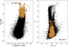 |
Fig. B.1 Colour-magnitude diagrams of VIRAC2 and HST in the SWEEPS window. The orange points correspond to the location of the cross match after the quality cuts and 3σ clipping. |
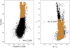 |
Fig. B.2 Colour-magnitude diagrams of VIRAC2 and HST in the Stanek window. The orange points correspond to the location of the cross match after the quality cuts and 3σ clipping. |
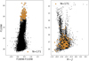 |
Fig. B.3 Colour-magnitude diagrams of VIRAC2 and HST in the Ogle29 window. The orange points correspond to the location of the cross match after the quality cuts and 3σ clipping. |
Appendix C Proper motion comparison between Gaia DR3 and HST
In this section, we show the uncertainty normalised proper motion differences (Δμ/σμ) between Gaia DR3 and HST for the BTP-Stanek window, the BTP-Ogle29 window, ω Cen F1, ω Cen F2, ω Cen F3, and NGC 6652. Figures C.1, C.2, C.3, C.4, C.5, and C.6 are the equivalent to Fig. 4, where the left and right panels correspond to Δμ/σμ in RA and Dec, respectively.
Appendix D Variation of r in the BTP
We explored the variation in the inflation factor when we adopted an upper limit in the BTP PM uncertainties different than 0.3 mas yr−1, within the range 0.3 − 1 mas yr−1. This was to account for HST systematics, which we cannot quantify in the data. For the Stanek and Ogle29 data sets, the inflation factor is reduced up to 20% when we assume a BTP PM uncertainty of 0.6 mas yr−1, and up to 50% when we assume a BTP PM uncertainty of 1 mas yr−1 . However, for the SWEEPS data set, the inflation factor is reduced by only 25% assuming a PM uncertainty of 1 mas yr−1. The results are summarised in Figure D.1.
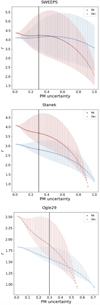 |
Fig. D.1 Variation in r in the BTP fields for different upper limits of PM uncertainties. The PM uncertainty is given in mas yr−1. The points are the median r at a given σμ, and the vertical lines mark the range between the 16th and 84th percentiles. |
Appendix E Comparison of other fields with the extended SWEEPS catalogue
In this section, we extend the discussion of Sect.4.2. The extended SWEEPS catalogue (Calamida et al. 2014) is based on observations of the BTP-SWEEPS window with additional epochs that extended the time baseline, which led to more accurate measurements with well-characterised individual uncertainties. This data set provides an opportunity to internally validate the BTP-SWEEPS data. The median inflation factor of the SWEEPS extended catalogue computed in different magnitude bins is labelled SWEEPS C14 in Fig. E.1. The median inflation factor is consistent with that of the BTP-SWEEPS window adopting a PM uncertainty upper limit of 0.3 mas yr−1. The exception is found for the brightest bin in the Dec component (G < 18.5), where some sources may have poor quality, but we cannot filter them because the extended SWEEPS catalogue lacks quality flags.
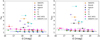 |
Fig. E.1 Dependence of the inflation factor r on G-band magnitude of the studied HST fields. Same as Fig. 5, but with the addition of the SWEEPS extended catalogue (SWEEPS C14 in the label). The points represent the medians of the magnitude bins, and for r, the error bars are those of the 16th and 84th percentiles. The bars in G indicate the magnitude distribution in a given bin, where the marker is the median. |
References
- Alonso-García, J., Saito, R. K., Hempel, M., et al. 2018, A & A, 619, A4 [Google Scholar]
- Arenou, F., Luri, X., Babusiaux, C., et al. 2018, A & A, 616, A17 [NASA ADS] [CrossRef] [EDP Sciences] [Google Scholar]
- Astropy Collaboration (Robitaille, T. P., et al.) 2013, A & A, 558, A33 [NASA ADS] [CrossRef] [EDP Sciences] [Google Scholar]
- Astropy Collaboration (Price-Whelan, A. M., et al.) 2018, AJ, 156, 123 [Google Scholar]
- Babusiaux, C., & Gilmore, G. 2005, MNRAS, 358, 1309 [NASA ADS] [CrossRef] [Google Scholar]
- Babusiaux, C., Fabricius, C., Khanna, S., et al. 2023, A & A, 674, A32 [Google Scholar]
- Barbuy, B., Chiappini, C., & Gerhard, O. 2018, ARA & A, 56, 223 [Google Scholar]
- Battaglia, G., Taibi, S., Thomas, G. F., & Fritz, T. K. 2022, A & A, 657, A54 [Google Scholar]
- Bellini, A., Anderson, J., & Bedin, L. R. 2011, PASP, 123, 622 [CrossRef] [Google Scholar]
- Bellini, A., Anderson, J., Bedin, L. R., et al. 2017, ApJ, 842, 6 [NASA ADS] [CrossRef] [Google Scholar]
- Bellini, A., Libralato, M., Bedin, L. R., et al. 2018, ApJ, 853, 86 [NASA ADS] [CrossRef] [Google Scholar]
- Bernard, E. J., Schultheis, M., Di Matteo, P., et al. 2018, MNRAS, 477, 3507 [CrossRef] [Google Scholar]
- Brown, T. M., Sahu, K., Zoccali, M., et al. 2009, AJ, 137, 3172 [NASA ADS] [CrossRef] [Google Scholar]
- Calamida, A., Sahu, K. C., Anderson, J., et al. 2014, ApJ, 790, 164 [NASA ADS] [CrossRef] [Google Scholar]
- Cantat-Gaudin, T., Fouesneau, M., Rix, H.-W., et al. 2023, A & A, 669, A55 [Google Scholar]
- Chatzopoulos, S., Fritz, T. K., Gerhard, O., et al. 2015, MNRAS, 447, 948 [Google Scholar]
- Clarke, J. P., & Gerhard, O. 2022, MNRAS, 512, 2171 [NASA ADS] [CrossRef] [Google Scholar]
- Clarke, J. P., Wegg, C., Gerhard, O., et al. 2019, MNRAS, 489, 3519 [Google Scholar]
- Clarkson, W., Sahu, K., Anderson, J., et al. 2008, ApJ, 684, 1110 [NASA ADS] [CrossRef] [Google Scholar]
- Clarkson, W. I., Calamida, A., Sahu, K. C., et al. 2018, ApJ, 858, 46 [NASA ADS] [CrossRef] [Google Scholar]
- del Pino, A., Libralato, M., van der Marel, R. P., et al. 2022, ApJ, 933, 76 [NASA ADS] [CrossRef] [Google Scholar]
- El-Badry, K., Rix, H.-W., & Heintz, T. M. 2021, MNRAS, 506, 2269 [NASA ADS] [CrossRef] [Google Scholar]
- Everall, A., & Boubert, D. 2022, MNRAS, 509, 6205 [Google Scholar]
- Fabricius, C., Luri, X., Arenou, F., et al. 2021, A & A, 649, A5 [Google Scholar]
- Feldmeier-Krause, A., Neumayer, N., Schödel, R., et al. 2015, A & A, 584, A2 [Google Scholar]
- Fragkoudi, F., Grand, R. J. J., Pakmor, R., et al. 2020, MNRAS, 494, 5936 [Google Scholar]
- Gaia Collaboration (Brown, A. G. A., et al.) 2021, A & A, 649, A1 [NASA ADS] [CrossRef] [EDP Sciences] [Google Scholar]
- Gaia Collaboration (Vallenari, A., et al.) 2022, Gaia DR3 documentation, European Space Agency; Gaia Data Processing and Analysis Consortium, online at https://gea.esac.esa.int/archive/documentation/GDR3/index.html, 19 [Google Scholar]
- Garro, E. R., Minniti, D., Gómez, M., et al. 2022, A & A, 662, A95 [Google Scholar]
- Gillessen, S., Eisenhauer, F., Fritz, T. K., et al. 2009, ApJ, 707, L114 [Google Scholar]
- Gonzalez, O. A., Rejkuba, M., Zoccali, M., et al. 2012, A & A, 543, A13 [Google Scholar]
- Gonzalez, O. A., Rejkuba, M., Zoccali, M., et al. 2013, A & A, 552, A110 [NASA ADS] [CrossRef] [EDP Sciences] [Google Scholar]
- Gonzalez, O. A., Zoccali, M., Debattista, V. P., et al. 2015, A & A, 583, L5 [Google Scholar]
- GRAVITY Collaboration (Abuter, R., et al.) 2018, A & A, 615, L15 [Google Scholar]
- GRAVITY Collaboration (Abuter, R., et al.) 2020, A & A, 636, L5 [Google Scholar]
- Harris, C. R., Millman, K. J., van der Walt, S. J., et al. 2020, Nature, 585, 357 [NASA ADS] [CrossRef] [Google Scholar]
- Horta, D., Schiavon, R. P., Mackereth, J. T., et al. 2021, MNRAS, 500, 1385 [Google Scholar]
- Johnson, C. I., Rich, R. M., Fulbright, J. P., Valenti, E., & McWilliam, A. 2011, ApJ, 732, 108 [NASA ADS] [CrossRef] [Google Scholar]
- Kader, J. A., Pilachowski, C. A., Johnson, C. I., et al. 2022, ApJ, 940, 76 [NASA ADS] [CrossRef] [Google Scholar]
- Kozhurina-Platais, V., & Martlin, C. 2021, Accuracy of the HST/WFC3 Standard Astrometric Catalog w.r.t Gaia EDR3, Instrument Science Report WFC3 2021-07, 18 [Google Scholar]
- Kunder, A., Rich, R. M., Koch, A., et al. 2016, ApJ, 821, L25 [CrossRef] [Google Scholar]
- Libralato, M., Bellini, A., Bedin, L. R., et al. 2018, ApJ, 854, 45 [NASA ADS] [CrossRef] [Google Scholar]
- Libralato, M., Bellini, A., Vesperini, E., et al. 2022, ApJ, 934, 150 [NASA ADS] [CrossRef] [Google Scholar]
- Lindegren, L., Lammers, U., Bastian, U., et al. 2016, A & A, 595, A4 [NASA ADS] [CrossRef] [EDP Sciences] [Google Scholar]
- Lindegren, L., Hernández, J., Bombrun, A., et al. 2018, A & A, 616, A2 [NASA ADS] [CrossRef] [EDP Sciences] [Google Scholar]
- Lindegren, L., Bastian, U., Biermann, M., et al. 2021a, A & A, 649, A4 [Google Scholar]
- Lindegren, L., Klioner, S. A., Hernández, J., et al. 2021b, A & A, 649, A2 [Google Scholar]
- Lucey, M., Hawkins, K., Ness, M., et al. 2021, MNRAS, 501, 5981 [NASA ADS] [CrossRef] [Google Scholar]
- Luna, A., Minniti, D., & Alonso-García, J. 2019, ApJ, 887, L39 [NASA ADS] [CrossRef] [Google Scholar]
- Maiz Apellániz, J., Pantaleoni González, M., & Barbá, R. H. 2021, A & A, 649, A13 [Google Scholar]
- Marchetti, T., Johnson, C. I., Joyce, M., et al. 2022, A & A, 664, A124 [Google Scholar]
- Massari, D., Breddels, M. A., Helmi, A., et al. 2018, Nat. Astron., 2, 156 [Google Scholar]
- Massari, D., Helmi, A., Mucciarelli, A., et al. 2020, A & A, 633, A36 [Google Scholar]
- McWilliam, A., & Zoccali, M. 2010, ApJ, 724, 1491 [NASA ADS] [CrossRef] [Google Scholar]
- Minniti, D., Lucas, P. W., Emerson, J. P., et al. 2010, New A, 15, 433 [Google Scholar]
- Nataf, D. M., Udalski, A., Gould, A., Fouqué, P., & Stanek, K. Z. 2010, ApJ, 721, L28 [NASA ADS] [CrossRef] [Google Scholar]
- Nataf, D. M., Gonzalez, O. A., Casagrande, L., et al. 2016, MNRAS, 456, 2692 [Google Scholar]
- Ness, M., & Lang, D. 2016, AJ, 152, 14 [NASA ADS] [CrossRef] [Google Scholar]
- Nidever, D. L., Zasowski, G., & Majewski, S. R. 2012, ApJS, 201, 35 [NASA ADS] [CrossRef] [Google Scholar]
- Nogueras-Lara, F. 2022, A & A, 666, A72 [Google Scholar]
- Nogueras-Lara, F., Schödel, R., Gallego-Calvente, A. T., et al. 2020, Nat. Astron., 4, 377 [Google Scholar]
- Nogueras-Lara, F., Schödel, R., & Neumayer, N. 2021, A & A, 653, A133 [Google Scholar]
- Pedregosa, F., Varoquaux, G., Gramfort, A., et al. 2011, J. Mach. Learn. Res., 12, 2825 [Google Scholar]
- Pfuhl, O., Fritz, T. K., Zilka, M., et al. 2011, ApJ, 741, 108 [Google Scholar]
- Portail, M., Gerhard, O., Wegg, C., & Ness, M. 2017, MNRAS, 465, 1621 [NASA ADS] [CrossRef] [Google Scholar]
- Riello, M., De Angeli, F., Evans, D. W., et al. 2021, A & A, 649, A3 [Google Scholar]
- Rix, H.-W., Chandra, V., Andrae, R., et al. 2022, ApJ, 941, 45 [NASA ADS] [CrossRef] [Google Scholar]
- Rybizki, J., Green, G. M., Rix, H.-W., et al. 2022, MNRAS, 510, 2597 [NASA ADS] [CrossRef] [Google Scholar]
- Sahu, K. C., Casertano, S., Bond, H. E., et al. 2006, Nature, 443, 534 [Google Scholar]
- Saito, R. K., Hempel, M., Minniti, D., et al. 2012, A & A, 537, A107 [Google Scholar]
- Sanders, J. L., Smith, L., González-Fernández, C., Lucas, P., & Minniti, D. 2022, MNRAS, 514, 2407 [CrossRef] [Google Scholar]
- Scalco, M., Bellini, A., Bedin, L. R., et al. 2021, MNRAS, 505, 3549 [NASA ADS] [CrossRef] [Google Scholar]
- Schödel, R., Feldmeier, A., Neumayer, N., Meyer, L., & Yelda, S. 2014, Class. Quantum Gravity, 31, 244007 [CrossRef] [Google Scholar]
- Schultheis, M., Chen, B. Q., Jiang, B. W., et al. 2014, A & A, 566, A120 [NASA ADS] [CrossRef] [EDP Sciences] [Google Scholar]
- Shahzamanian, B., Schödel, R., Nogueras-Lara, F., et al. 2022, A & A, 662, A11 [Google Scholar]
- Simion, I. T., Belokurov, V., Irwin, M., et al. 2017, MNRAS, 471, 4323 [NASA ADS] [CrossRef] [Google Scholar]
- Smith, L. C., Lucas, P. W., Kurtev, R., et al. 2018, MNRAS, 474, 1826 [Google Scholar]
- Stanek, K. Z., Mateo, M., Udalski, A., et al. 1994, ApJ, 429, L73 [NASA ADS] [CrossRef] [Google Scholar]
- Surot, F., Valenti, E., Gonzalez, O. A., et al. 2020, A & A, 644, A140 [Google Scholar]
- Vasiliev, E., & Baumgardt, H. 2021, MNRAS, 505, 5978 [NASA ADS] [CrossRef] [Google Scholar]
- Virtanen, P., Gommers, R., Oliphant, T. E., et al. 2020, Nat. Methods, 17, 261 [Google Scholar]
- Wegg, C., & Gerhard, O. 2013, MNRAS, 435, 1874 [Google Scholar]
- Wylie, S. M., Clarke, J. P., & Gerhard, O. E. 2022, A & A, 659, A80 [Google Scholar]
- Zhang, M., & Kainulainen, J. 2022, MNRAS, 517, 5180 [NASA ADS] [CrossRef] [Google Scholar]
- Zoccali, M. 2019, Boletin de la Asociacion Argentina de Astronomia La Plata Argentina, 61, 137 [NASA ADS] [Google Scholar]
- Zoccali, M., & Valenti, E. 2016, PASA, 33, e025 [NASA ADS] [CrossRef] [Google Scholar]
- Zoccali, M., Renzini, A., Ortolani, S., et al. 2003, A & A, 399, 931 [NASA ADS] [CrossRef] [EDP Sciences] [Google Scholar]
Throughout this work, the bulge includes the 300 deg2 region in −10deg < l < 10 deg and −10 deg < b < 5 deg, comprising a radius of ~2.5 kpc around the Galactic centre.
Version 2 high-level science products from GO-11664.
The authors propose an additional cut: the absolute value of the corrected excess factor (phot_bp_rp_excess_factor) within 5σ at the corresponding G-band magnitude (see Eqs. (6) and (18) of Riello et al. 2021). However, this cut pertains to photometric reliability, and because we deal with astrometry in this study, we decided not to take it into account in order to increase the statistics.
All Tables
Galactic coordinates, extinction coefficient, and the final number of matched sources (Nf) used for the analysis of the four BTP low-reddening windows; the outskirt fields of ωCen, F1, F2, and F3; and the globular cluster NGC 6652.
Median inflation factor (r) in a given G-band magnitude range for the seven studied fields.
Number of sources in Gaia DR3 in a given field, area of the field, and median values of the inflation factor r.
Median inflation factor (r) in a given J-band magnitude range for the seven studied fields.
All Figures
|
Fig. 1 Gaia DR3 G-band and HST F555W magnitude difference. The initial position cross match is refined with a selection of stars that have similar magnitudes. The good matches are below the solid red line at F555W − G = 1. |
| In the text | |
|
Fig. 2 Number of sources in Gaia DR3 and HST-BTP in the SWEEPS field. From top to bottom: Initial sample in the same FoV after applying the quality cuts described in Sect. 2, after a cross match between the data sets with a tolerance of 0.″5, and the final sample used for the study. The position of the sources in the final sample is plotted in orange. In the second row, the lack of sources in the corners of the BTP data set arises because they did not have a proper motion value in the BTP catalogue. This is due to small differences in the field orientation between different epoch exposures. |
| In the text | |
|
Fig. 3 Colour-magnitude diagrams of Gaia DR3 and HST in the SWEEPS window. The orange points correspond to the location of the cross-matched sources after the quality cuts and a 3σ clipping in the uncertainty normalised proper motion difference. The black dots are the total sources in the field after the quality cuts. The two catalogues overlap in a short magnitude range. |
| In the text | |
|
Fig. 4 Normalised proper motion difference distribution for the SWEEPS field. The dashed curves are the initial distributions in each coordinate component. The solid curves are the distributions after Gaia DR3 proper motion uncertainties are multiplied by the inflation factor r. The standard deviation of the distribution before and after applying the inflation factor is labelled Κ and σ, respectively. |
| In the text | |
|
Fig. 5 Dependence of the inflation factor r on the G-band magnitude of the studied HST fields. The points represent the medians of the magnitude bins, and for r, the error bars are the 16th and 84th percentiles. The bars in G indicate the magnitude distribution in a given bin, where the marker is the median. The plotted data are listed in Table 2. |
| In the text | |
|
Fig. 6 Normalised proper motion difference distribution for VIRAC2 vs. SWEEPS-BTP (top), VIRAC2 vs. Stanek-BTP (middle), and VIRAC2 vs. Ogle29-BTP (bottom). The dashed curves are the initial distributions in each coordinate component. The solid curves are the distributions after the VIRAC2 uncertainties are multiplied by the inflation factor r. |
| In the text | |
|
Fig. 7 Dependence of the inflation factor r on the number density defined for sources found in the Gaia DR3 catalogue in a given field. The median r for the different fields is plotted with different colours. The error bars correspond to the 16th and 84th percentile in the distribution of r across the magnitude range of a given field. The shade is the 1σ uncertainty on the fit. The plotted data are listed in Table 3. |
| In the text | |
|
Fig. 8 Dependence of the inflation factor on the Gaia and HST uncertainty ratio. The vertical line marks σGaia = σΗSΤ. For sources with σGaia > σΗSΤ, the inflation factor asymptotically reaches a minimum value that corresponds to the standard deviation K of the parent population. This behaviour follows the functional form of Eq. (3). |
| In the text | |
|
Fig. 9 Dependence of the inflation factor r on VIRAC2 J magnitude. The proper motion comparison was made between VIRAC2 and the HST-BTP SWEEPS, Stanek, and Ogle29 windows. The points are the median values of J in each magnitude bin, and the error bars indicate the magnitude distribution at a given bin. In r, the error bars are the 16th and 84th percentile. |
| In the text | |
|
Fig. A.1 Colour-magnitude diagrams of Gaia and HST in the Stanek window. The orange points correspond to the location of the cross match after the quality cuts and 3σ clipping. |
| In the text | |
|
Fig. A.2 Colour-magnitude diagrams of Gaia and HST in the Ogle29 window. The orange points correspond to the location of the cross match after the quality cuts and 3σ clipping. |
| In the text | |
|
Fig. A.3 Colour-magnitude diagrams of Gaia and HST in the Baade window. The orange points correspond to the location of the cross match after the quality cuts and 3σ clipping. |
| In the text | |
|
Fig. A.4 Colour-magnitude diagrams of Gaia and HST in the ω Cen F1 field. The orange points correspond to the location of the cross match after the quality cuts and 3σ clipping. |
| In the text | |
|
Fig. A.5 Colou-magnitude diagrams of Gaia and HST in the ω Cen F2 field. The orange points correspond to the location of the cross match after the quality cuts and 3σ clipping. |
| In the text | |
|
Fig. A.6 Colour-magnitude diagrams of Gaia and HST in the ω Cen F3 field. The orange points correspond to the location of the cross match after the quality cuts and 3σ clipping. |
| In the text | |
|
Fig. A.7 Colour-magnitude diagrams of Gaia and HST in the globular cluster NGC 6652. The orange points correspond to the location of the cross match after the quality cuts and 3σ clipping. |
| In the text | |
|
Fig. B.1 Colour-magnitude diagrams of VIRAC2 and HST in the SWEEPS window. The orange points correspond to the location of the cross match after the quality cuts and 3σ clipping. |
| In the text | |
|
Fig. B.2 Colour-magnitude diagrams of VIRAC2 and HST in the Stanek window. The orange points correspond to the location of the cross match after the quality cuts and 3σ clipping. |
| In the text | |
|
Fig. B.3 Colour-magnitude diagrams of VIRAC2 and HST in the Ogle29 window. The orange points correspond to the location of the cross match after the quality cuts and 3σ clipping. |
| In the text | |
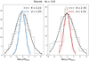 |
Fig. C.1 Same as Fig. 4, but for the Stanek window. |
| In the text | |
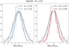 |
Fig. C.2 Same as Fig. 4, but for the Ogle29 window. |
| In the text | |
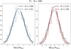 |
Fig. C.3 Same as Fig. 4, but for the ω Cen F1 field. |
| In the text | |
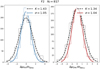 |
Fig. C.4 Same as Fig. 4, but for the ω Cen F2 field. |
| In the text | |
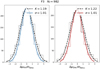 |
Fig. C.5 Same as Fig. 4, but for the ω Cen F3 field. |
| In the text | |
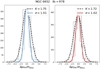 |
Fig. C.6 Same as Fig. 4, but for the globular cluster NGC 6652. |
| In the text | |
|
Fig. D.1 Variation in r in the BTP fields for different upper limits of PM uncertainties. The PM uncertainty is given in mas yr−1. The points are the median r at a given σμ, and the vertical lines mark the range between the 16th and 84th percentiles. |
| In the text | |
|
Fig. E.1 Dependence of the inflation factor r on G-band magnitude of the studied HST fields. Same as Fig. 5, but with the addition of the SWEEPS extended catalogue (SWEEPS C14 in the label). The points represent the medians of the magnitude bins, and for r, the error bars are those of the 16th and 84th percentiles. The bars in G indicate the magnitude distribution in a given bin, where the marker is the median. |
| In the text | |
Current usage metrics show cumulative count of Article Views (full-text article views including HTML views, PDF and ePub downloads, according to the available data) and Abstracts Views on Vision4Press platform.
Data correspond to usage on the plateform after 2015. The current usage metrics is available 48-96 hours after online publication and is updated daily on week days.
Initial download of the metrics may take a while.