| Issue |
A&A
Volume 677, September 2023
|
|
|---|---|---|
| Article Number | A107 | |
| Number of page(s) | 18 | |
| Section | Interstellar and circumstellar matter | |
| DOI | https://doi.org/10.1051/0004-6361/202345968 | |
| Published online | 13 September 2023 | |
Toward a 3D kinetic tomography of Taurus clouds
II. A new automated technique and its validation★
1
GEPI, Observatoire de Paris, Université PSL, CNRS,
5 Place Jules Janssen,
92190
Meudon,
France
e-mail: This email address is being protected from spambots. You need JavaScript enabled to view it.
2
ACRI-ST,
260 route du Pin Montard,
06904,
Sophia Antipolis,
France
3
Univ. Grenoble Alpes, CNRS, IPAG,
38000
Grenoble,
France
4
Canadian Institute for Theoretical Astrophysics, University of Toronto,
60 St. George Street,
Toronto, ON
M5S 3H8,
Canada
Received:
21
January
2023
Accepted:
3
April
2023
Abstract
Context. Three-dimensional (3D) kinetic maps of the Milky Way interstellar medium are an essential tool in studies of its structure and of star formation.
Aims. We aim to assign radial velocities to Galactic interstellar clouds now spatially localized based on starlight extinction and star distances from Gaia and stellar surveys.
Methods. We developed an automated search for coherent projections on the sky of clouds isolated in 3D extinction density maps on the one hand, and regions responsible for CO radio emissions at specific Doppler shifts on the other hand. The discrete dust structures were obtained by application of the Fellwalker algorithm to a recent 3D extinction density map. For each extinction cloud, a technique using a narrow sliding spectral window moved along the contour-bounded CO spectrum and geometrical criteria was used to select the most likely velocity interval.
Results. We applied the new contour-based technique to the 3D extinction density distribution within the volume encompassing the Taurus, Auriga, Perseus, and California molecular complexes. From the 45 clouds issued from the decomposition, 42 were assigned a velocity. The remaining structures correspond to very weak CO emission or extinction. We used the non-automated assignments of radial velocities to clouds of the same region presented in Paper I and based on KI absorption spectra as a validation test. The new fully automated determinations were found to be in good agreement with these previous measurements.
Conclusions. Our results show that an automated search based on cloud-contour morphology can be efficient and that this novel technique may be extended to wider regions of the Milky Way and at larger distance. We discuss its limitations and potential improvements after combination with other techniques.
Key words: dust, extinction / ISM: lines and bands / ISM: structure / local insterstellar matter
Full Table 2 is available at the CDS via anonymous ftp to cdsarc.cds.unistra.fr (130.79.128.5) or via https://cdsarc.cds.unistra.fr/viz-bin/cat/J/A+A/677/A107
© The Authors 2023
 Open Access article, published by EDP Sciences, under the terms of the Creative Commons Attribution License (https://creativecommons.org/licenses/by/4.0), which permits unrestricted use, distribution, and reproduction in any medium, provided the original work is properly cited.
This article is published in open access under the Subscribe to Open model. This email address is being protected from spambots. You need JavaScript enabled to view it. to support open access publication.
1 Introduction
Three-dimensional (3D) kinetic tomography of the interstellar medium (ISM), that is, the assignment of radial or 3D velocities to interstellar structures, is a multi-scale tool in star formation studies. On small scales and Milky Way ISM observations, it helps in linking the extremely detailed multiwavelength, mul-tispecies emission measurements with localized structures and allows us to understand the respective roles of self gravity, converging flows and turbulence, magnetic field, and chains of reactions following the first star births. On a large scale, 3D kinetic tomography allows the role of global dynamics and spiral arms to be distinguished from that of local structure and the local stellar population. Importantly, 3D kinetic maps of the ISM would be especially useful when used in conjunction with Gaia-based 3D kinetic maps of the Milky Way stars under development. The use of the Galactic rotation curve, although convenient for locating distant Galactic interstellar clouds, is not very helpful in the aforementioned detailed studies due to limited realism and the lack of detection of peculiar and therefore particularly interesting velocities, and is not applicable toward the Galactic center (Wenger et al. 2018; Peek et al. 2022). Fortunately, massive stellar surveys with new generation spectro-graphs, new detailed radio emission spectral data, and, last but not least, parallaxes and photometric data from the Gaia mission, all emerging during the last two decades, are currently bringing huge amounts of data that can be used in 3D kinetic tomography computations. Combinations of astrometric and/or photometric distances with absorption or extinction measurements feed the construction of 3D distributions of dust or gaseous species, and, in turn, these distributions can be combined with emission spectra to obtain 3D kinetic information.
Thanks to this favorable context, 3D kinetic tomography of the Galactic ISM was recently worked out in several ways. Each of the techniques has its own strengths and limitations. A detailed introduction to kinetic tomography is given by Tchernyshyov & Peek (2017), and additional descriptions and references are given in the articles cited below. A first approach is the combination of dust extinction data and radio emission spectra. Tchernyshyov & Peek (2017) developed a method using H I and CO spectral data (i.e. position-position-velocity (PPV) cubes) on the one hand and cumulative reddening radial profiles derived from PansSTARRS and 2MASS on the other. Each spatial cell along a radial profile is assigned a Gaussian velocity distribution. The mean velocity is allowed to fluctuate around the value predicted by a radially varying rotation curve, the velocity dispersion is limited to a range of classical values, and the velocity dispersion around this value has imposed limits. Conversion factors from CO equivalent width to H column and from H column to reddening are imposed. The adjustment of the model to the emission data is regularized to avoid strong variations among neighboring cells. The technique has the advantage of being applicable everywhere, but does not always allow two (or more) clouds of similar dust opacity located at different distances and with different radial velocities to be disentangled, despite the regularization. A different method was developed by Zucker et al. (2018) who extended the Green et al. (2018) Bayesian technique for reddening-profile determination from individual extinctions by fitting a linear combination of 12CO velocity slices to the major reddening steps corresponding to the densest structures in Perseus. The authors were able to assign radial velocities and distances to those structures in a very precise way. The limitation here is due to the need for hypotheses about the absence of CO associated with the clouds in front of and beyond the considered region.
A second category of kinetic tomography is based on massive amounts of stellar spectra and makes use of both interstellar absorption Doppler shifts and target distances. Tchernyshyov et al. (2018) used Doppler shifts and strengths of a near-infrared diffuse interstellar band (DIB) extracted from SDSS/APOGEE stellar spectra in combination with photometric distances of the target stars to derive a large-scale planar map of the radial velocity. The advantage of the method is the lack of ambiguities, as the parallel evolutions are followed with the distance of the DIB radial velocity and of the DIB strength. Potential limitations of this method may arise from the variability of the DIB-to-extinction ratio. However, according to Puspitarini et al. (2015), such variability should not have significant consequences on the tomography. These authors used two different DIBs in the visible range and their measurements in a series of directions, and found very similar radial profiles of the strengths of the two DIBs as well as of dust extinction. On the other hand, there are limitations to the achievable velocity resolution as a result of the non-negligible intrinsic width of the DIB. For example, there is a limit of ≃10 km s−1 in the case of the APOGEE DIB. Finally, the technique is still limited by the relatively low number of target stars for which high-spectral-resolution, high signal spectra are available. Ivanova et al. (2021; Paper I) attempted to use a hybrid method also based on absorption data, but this time in combination with 3D extinction maps. The authors used neutral potassium absorption data in a series of stars distributed within ≃600 pc in the anti-center area encompassing the Taurus, Auriga, Perseus, and California clouds (hereafter referred to as the Taurus clouds) to derive partial information on the velocity field in a non-automated way. The kinematic information extracted in this way could benefit from high spectral resolution and the choice of narrow and strong absorption lines (the 766.5 and 770.0 nm KI lines) to ensure ease of detection and Doppler shift precision. On the other hand, the very limited number of targets and their small spatial density led to a restricted study. Nevertheless, this latter study provides a validation test for the new automated technique described in the present article. In all techniques based on absorption lines or bands, massive spectroscopic surveys with high sky coverage would be necessary to extend the 3D kinetic mapping.
A third and completely different approach uses the fact that newly born stars share the motion of their parent interstellar clouds. Galli et al. (2019) developed and applied clustering algorithms to identify groups of young stellar objects (YSOs) in Taurus star-forming areas and derived their distances and 3D motions based on VLBI astrometry, Gaia parallaxes, and proper motions. These authors verified the similarity between the radial velocities of each cluster and that of the associated molecular cloud, providing distance assignment to the clouds and newly born stars. This technique allows high accuracy to be achieved on distances and velocities, but is limited to star forming regions. In addition, infrared data are needed for the very young objects linked to their parent cloud due to the very strong dust opacity and extinction in the visible.
In this work, we explored a different, automated technique. This novel method uses CO emission spectra and 3D dust extinction density maps. It is based on the resemblance between the projection of a cloud on the sky and the extent and shape of a series of mono-kinetic CO emission maps. We applied this cloud-contour-based technique to the volume encompassing the nearby anti-center Taurus clouds. The difficulty in performing kinetic tomography in a region where dense clouds extend in distance and with overlapping 2D projections with a relatively narrow range of velocities (i.e., less than –15 to +15 km s−1) led us to choose these clouds as test cases to evaluate our method. This choice was also especially motivated by the availability of the aforementioned results recently obtained by Ivanova et al. (2021), which allow us to perform a thorough validation. An additional reason for the choice of this region is its latitude range and the subsequent limited distance to the clouds (less than ≃1 kpc for b < −3 deg), which ensures their inclusion in the used 3D extinction density map. Finally, as mentioned above, the choice of these clouds is not guided by the search for an easy case. On the contrary, this region is very complex and has characteristics that make kinetic tomography especially difficult. We know that in the particular case of two (or more) clouds at distributed distances and with identical projections on the sky, assignment of the two (or more) radial velocities measured in their directions is not possible if these assignments are based on morphology only. With our study, we aim to evaluate the frequency of such cases of indeterminacy, or equivalently the applicability of a technique solely based on projection geometry to complex regions such as the Taurus area.
The paper is organized as follows. Section 2 presents the data used as sources for our technical study. Section 3.1 describes how the CO data are denoised by means of the ROHSA code (Marchal et al. 2019) and are used to create a restriction mask necessary for the following step. Section 3 presents the decomposition of the masked dust distribution into distinct 3D structures. Sections 4 and 5 detail the newly developed technique of velocity assignment to the dust structures and the results. Sections 6 and 7 discuss our comparisons with other independent results, as well as limitations and potential extensions of the method.
2 Data
2.1 CO data
We made use of radio 12CO spectral cubes taken from the well-known series of data assembled by Dame et al. (2001). In the Taurus area, the angular resolution is ≃0.125° and the CO emission spectrum is decomposed into channels of 1.3 km s−1 each. The limits of the main region containing Taurus, Auriga, Perseus, and California are [150°, 185°] in longitude and [−30°, 0°] in latitude. The characteristic noise for Taurus according to Dame et al. (2001) is ≃0.25 K.
This CO dataset was used at two different steps in the whole procedure and in two different ways. First, it was used to delimit regions of the sky in the direction of CO clouds (see Sect. 3.1). For this purpose, it was previously regularized and decomposed into discrete structures to avoid highly irregular contours in the resulting mask. Second, it was used in its initial state during the association phase described in Sect. 4.
As we demonstrate below, the angular and velocity resolutions of the CO data are suited to our study given the minimum size of the dust clouds (see below). The main limitation here come from the noise level.
2.2 Extinction density maps
We used a 3D distribution of extinction density based on work presented by Lallement et al. (2022) and Vergely et al. (2022). The map is computed through tomographic inversion of large amounts of extinction–distance pairs for stars distributed in both direction and distance, producing the extinction per unit distance that photons suffer when traveling at a given location in 3D space, a quantity that is proportional to the dust volume density at this point. The map is based on 35 million distance–extinction measurements based on Gaia parallaxes and Gaia plus 2MASS photometric data augmented by 6 million measurements from published catalogs based on spectroscopy and photometry. To overcome the strong under-determination aspect of the full 3D inversion (distribution in each point in space based on a limited number of lines of sight), a regularization is performed that takes the form of a spatial covariance kernel or minimum size of structures. In order to maximize the achieved spatial resolution (minimum kernel), an iterative, hierarchical method is used, which is in the form of a series of inversions at increasing resolution. In regions where the target space density is high, the kernel width is reduced, while prior results are kept where the target density is scarce and does not allow further kernel reduction. For details of the inversion method and descriptions of the recent maps, readers can refer to Lallement et al. (2019) and Vergely et al. (2022). We have used the latest and most precise map for which the final (minimum) kernel width is 10 pc. This resolution is achieved in a large fraction of the volume that is considered here. The map is discretized into voxels of 5 × 5 × 5 pc3 and the unit of the 550 nm extinction density is mag pc−1. The minimum size of the inverted dust structures will be the main limiting factor of our study.
In addition to the limitations on the spatial resolution associated with the limits on the target spatial density and the resulting local kernel, there is a second mapping limitation associated with lack of completeness in target brightness. As illustrated in Fig. 1, there is a lack of target stars located behind the most opaque cloud cores in the input catalog of distance–extinction pairs, simply because foreground extinction makes them too faint to possess measurable parallaxes and/or sufficiently accurate photometric or spectrometric data. As a result of the lack of strongly extincted targets, the reconstructed extinction density in the direction of the very dense cloud cores will be biased toward lower values than the actual ones, and this may affect dust-to-gas ratio estimates. However, the impact on our velocity assignment here is expected to be negligible, because we only use the cloud locations and their projected outer contours.
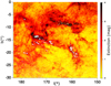 |
Fig. 1 Target stars used to build the 3D extinction density map in the Taurus area. The locations of the stars are shown as dots colored according to their extinction (color scale to the right of the figure). White areas correspond to high-opacity central regions within the main dust clouds (extinctions above ≃4 to 5 mag) and mark the subsequent lack of targets with precise distances and photometry due to their faintness. The reconstructed dust distribution will reproduce the clouds but underestimate the corresponding high opacity of the cores. |
3 Decomposition of the 3D extinction density map into individual clouds
3.1 CO-based restriction mask
Our choice of using CO, a tracer of the dense molecular clouds, implies that the dust associated with clouds made of only diffuse atomic gas cannot be part of an association with CO velocities. For this reason, we chose to eliminate clouds that have no CO emissions (to the best of our ability) in order to prevent unrealistic associations. To do so, we built and applied a restriction mask to our dust map before its decomposition into clumps. We assigned a null extinction density to all locations in 3D space whose projections on the sky are within regions with null CO emission. In other words, we carved or hollowed the 3D distribution. The mask does not eliminate atomic clouds located in the same direction as molecular clouds, but provides some useful limitation.
In what follows, we describe the method used to build the mask. The reasons for our choice are detailed and illustrated in Appendix A. First, we used the Gaussian decomposition algorithm ROHSA (Marchal et al. 2019) to denoise the CO data encompassing the neighboring anti-center clouds. In contrast to earlier applications dedicated to phase separation of 21 cm data (e.g., Marchal et al. 2021; Marchal & Miville-Deschênes 2021), ROHSA was used here for the spatial regularization it performs, which significantly reduces the noise. This regularization is a key step in the subsequent Fellwalker approach. The decomposition used in this work was obtained using N = 8 Gaussian functions and the hyper-parameters λα = λµ = λσ = 10, which controls the strength of the spatial regularization. As recommended in Marchal et al. (2019), the number of Gaussian components and the amplitude of these three hyper-parameters were chosen empirically so that the solution converges towards a noise-dominated residual.
The second step was the decomposition of the resulting CO data model into discrete elements in the (l, b, v) space based on the Fellwalker code (Hottier et al. 2021). This algorithm determines areas of high flux by looking for each path with sufficient gradient coming to a local maximum. All paths leading to the same maximum form a clump. To this end, we tuned the parameters of the Fellwalker algorithm as follows: We set the minimum value to be considered part of a clump to 0.20K, which is the standard deviation of values on this map, the maximum jump size to 3 voxels, and the minimum depth of valley between two neighboring peaks to 1 K. Here, voxels measure 0.125° × 0.125° × 1.3 km s−1.
The mask was finally defined as the full area of the projection on the sky of the totality of the retrieved elements resulting from the decomposition. Figure 2 shows the shape of this restriction mask. After superimposing this mask on a CO contour at 0.11 K.km s−1, we were able to check that it encompasses all the bright CO-emitting regions and goes further out over a small distance, where CO starts to be difficult to see. We note that, independently of the construction of the mask, this Fellwalker decomposition in (l, b, v) domains cannot be used for the velocity assignment because the algorithm does not allow two distinct clouds to share the same triplet (l, b, v), a situation commonly encountered in areas such as that considered here.
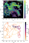 |
Fig. 2 Restriction mask and clump obtained. Top: restriction mask determined from the CO spectra (see Sect. 3.1) and applied to the 3D extinction map before its Fellwalker decomposition step. Masked areas are in black and superimposed on an image of the cumulative extinction integrated between 0 and 1 kpc within the inverted 3D extinction density distribution. The yellow contour corresponds to an integrated CO intensity of 0.11 K.km s−1. The unmasked areas encompass all regions where CO is present,includingareas of very weak intensityclose to the measurement uncertainty level, except very close to the Galactic Plane due to the limited size of the 3D map (see text). Bottom: projection in the same area of the discrete extinction clouds issued from the Fellwalker decomposition. Cloud contours are colored according to their mean distance from the Sun (right scale). |
3.2 Decomposition
As in Hottier et al. (2021), we chose to use the Fellwalker algorithm (Berry 2015) to extract individual structures from the 3D dust extinction density map. As explained above, we started with the modified extinction density map, in which non-null extinction voxels were restricted to non-masked directions (Fig 2). The gradient-based Fellwalker algorithm has the advantage of preventing the clustering from being dominated by radially elongated structures (the so-called fingers of God). Such features result from uncertainties on the distances of target stars and are common in 3D maps obtained by inversion. The radial gradients inside the fingers of God are almost flat, and therefore they can be filtered with the minimum gradient parameter. In the case of the extinction map used in this study, based on a hierarchical process and on the selection of accurate distances, the fingers of God are relatively limited. However, the cavities we created by application of the CO mask produce artificially elongated structures that mimic elongated fingers of God. We tuned the parameters of the algorithm as follows: we set the minimum threshold value to be considered part of a clump to 5.76 mmag, the jump maximum size to 2 voxels, the minimal gradient to 2.5mmag voxel−1, the clump outline size to 1 voxel, and the minimum depth of the valley between two neighboring peaks to half a standard deviation of the cube. We chose this last parameter in order to limit the merging step to the strict minimum. By doing so, we forced the algorithm to give us smaller clumps. We did this in order to obtain velocity variations of greater precision with our method, and because we are confident that it is robust enough to work well despite this over-division of our map. With this set of parameters, we sought to extract only the densest clumps and keep them as tight as possible, because we intended to compare their angular positions to CO emission, which has a better angular resolution than the extinction map. The threshold extinction value was computed from the threshold for the emission mask and the mean dust-to-CO ratio in Taurus, Perseus, and California from Lewis et al. (2022). Figure 2 shows the positions of the clumps in longitude and latitude coordinates. We can easily discern the three main features: Taurus and Auriga in the foreground, the more distant Perseus at l ∈ [155°, 160°] and b ∈ [−25°, −17°], and the most distant California at l ∈ [155°, 170°] and b ∈ [−11°, −4°], as well as some other isolated clumps. The figure also illustrates two types of decomposition. On the one hand, some clouds have overlapping projections, fully disconnected contours, and lie at significantly different distances. On the other hand, there are also pairs of neighboring clouds at the same distance that are adjacent to each other like two neighboring pieces of a puzzle; these clearly result from the division of a single, large volume into two distinct, smaller entities. This latter situation is due to our choice of the valley depth parameter. This will have an impact on our velocity assignment algorithm, as we show below.
4 Description of the velocity assignment method
Our goal is to assign a mean CO velocity to each 3D structure − previously extracted from the extinction map − based on the CO spectral cube. The velocity assignment is guided by the following considerations: if a cloud (hereafter central cloud or CC), either isolated or part of a contiguous, more extended structure (called EC; see below), is moving at a radial velocity Vi, then two conditions should be fulfilled. First, this velocity should correspond to an intensity level above the noise in the CO spectrum. Second, and most importantly, the angular area S(Vi) made by grouping all directions characterized by detectable CO emission at this specific velocity Vi should bear some resemblance to the CC or EC projection. Following these requirements, we first determined the series of velocities measured over the CC angular area, and then evaluated and ranked them based on geometrical criteria favoring a CC source. For each individual cloud CC, we performed the following operations.
4.1 Definitions
Definition of a median emission profile
We selected the set of lines of sight of the CO grid encompassed by the CC projected contours, and for each of them we extracted the individual CO temperature brightness profile as a function of LSR velocity from the CO spectral cube. Based on this series of spectra, we computed the median value over all points of the grid for each velocity channel and combined the results to build a median profile. This profile contains all velocity components present within at least half of the CC angular area that are associated to this central clump CC or to clouds in the foreground or in the background of this central cloud. This also includes components at the same velocity formed in spatially distinct clouds; in this case, the additional contributions of these clouds may result in a total presence of the velocity in more than half of the CC angular area. The noise level for the median profile is assumed to be 0.25 K, the average value estimated by Dame et al. (2001) in the Taurus region, divided by the square root of the number of lines of sight in the central clump.
Definition of the associated extended structure
As we choose to configure Fellwalker to have the smallest clumps possible, we need to treat clouds resulting from the decomposition that are sub-parts of a wide cloud by taking account of contiguous clumps where necessary when we come to use a presence criterion (see below) to assign a radial velocity. This is why we considered not only the central clump CC but also its close neighbors, if they exist. These close neighbors are defined as those clumps whose projections fully or partially overlap the CC area and whose barycenter is located within 25 pc of the barycen-ter of the central clump. This 25 pc limit is determined to be greater than the characteristic size of clumps, and smaller than the distance between two separate clouds. The combination of the central clump and those neighbors is the EC structure. In the case of an isolated cloud, the area of the EC reduces to that of the CC.
Definition of a test extended area
We considered a wide angular (WA) region encompassing the contours of the central clump and with an area of four times that of the central clump. To this end, we started with the smallest longitude-latitude rectangle containing the CC, and extended it by adding the same number of pixels in latitude and in longitude until its area reached four times that of the CC. The size of this region results from a compromise between the importance we want to give to the CC with respect to its angular environment, which favors a small area of the WA region, and the necessity to avoid cases in which the WA would appear too small because the EC covers an extended area around the CC. Our choice of four times the CC area does not totally prevent this latter situation from happening, but it guarantees that the CC is the main feature in the region.
Definition of a presence ratio for a velocity interval
The velocity interval (or window) is defined by its central velocity wi and its width measured in CO velocity channels. The criteria for the selection of the window and its central velocity wi are as follows: for each line of sight, we extracted the mean of the CO emission integrated along the window and compared it to the mean of the cloud median profile defined above. If the mean in the line of sight was greater than in the median profile and if the median profile at the central velocity had a greater brightness than the noise level of the median profile, we considered the velocity window as present along this line of sight (the line of sight is selected). We then repeated this computation for each line of sight within the WA, and computed the number of selected lines of sight interior to the neighborhood of the clump (EC) contours NECi on the one hand, and those interior to the whole WA NWAi on the other, as well as the ratio of these two numbers; that is, the ratio of the presence inside EC over the presence in WA, hereafter referred to as the presence ratio PECi:
 (1)
(1)
This selection process allows us, in principle, to discriminate between the velocity component(s) associated with the EC – for which we expect a grouping of the selected lines of sight within the EC contours – and the velocities associated with closer or more distant clouds – for which the majority of the selected lines of sight are not expected to be linked with the cloud projected area. In the same way, we defined the presence ratio specific to the central cloud alone PCCi:
 (2)
(2)
4.2 Velocity selection processes
Initial selection using a sliding window along the median profile
We moved a sliding window in LSR velocity along the CC median profile. The area emitting at velocities comprised within the window interval was used to estimate the presence ratio defined above. For this first step of velocity selection, we used a window of three velocity channels (for a total of 3.9 km s−1) in width, and a wider window of five velocity channels (for 6.5 km s−1) in order to cover the different widths of components. We retained the window center velocities with the two highest ratios and not located on adjacent velocity channels. More precisely, we first retained the center velocity with the highest ratio and then looked at the second best velocity that is not adjacent to the first. If no second best velocity passed our criterion, we simply retained the first as a prior. If no velocity passed our criterion, we rejected all velocity assignations for this clump. These first velocity intervals are too wide and too uncertain to be considered as components on their own, but they serve as the best priors for the next step, a multi-Gaussian fit of the median profile.
Velocity selections based on a Gaussian fit of the median profile
We performed a quadri-Gaussian fit of the median profile after having imposed, among the four components, the two velocities found at the previous step using a sliding window. We allowed these to vary within a narrow interval of 0.5 km s−1 in width. This process allowed us to identify between one and two additional potential velocity components, as illustrated in Fig. 3 for three different clouds, chosen as examples of the various configurations. More precisely, we first allowed two additional components, and if one of them was found to be redundant with another component, we removed it and allowed for only one additional Gaussian. These discrete fitted components (between 1 and 4 values) were used in the same way as the sliding windows for the computation of the presence ratio, that is for the same sky area and criteria of selection. The mean velocities of the third and fourth Gaussian components, which are generally much weaker than the two first, were allowed to vary in a larger interval than the first two (±30 km s−1) as they were the additional components that do not have any strong priors. We also limited the standard deviations of the Gaussians to a maximum of 1.3 km s−1.
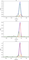 |
Fig. 3 Median emission profiles integrated within the projected contours of three clumps, numbered 8, 104, and 114 (black curves), and their fit with a multi-Gaussian function (blue curves). Individual Gaussian components of the function are also detailed in red, orange, green, and gray. The noise level of the profile is indicated by a dashed horizontal line. Clump 114 has a smaller angular size than the two others, which explains its higher noise level. |
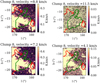 |
Fig. 4 Integrated emission between the velocity bounds of each Gaussian component (central velocity ± the standard deviation) for clump 8 (central velocities 8.8, 11.5, 7.2 and 4.1 km s−1 respectively). The yellow upper limit of the color scale corresponds to the emission level at which the component is considered to be present in the line of sight. The CC clump contours are shown in green and the contours of the neighboring clouds constituting EC are shown in red. |
Final velocity selection
Among the (up to) four fitted velocities, we selected the component with the highest product of the two presence ratios PPi = PECi × PCCi, which we call the presence product. The use of the presence product allowed us to give more weight to the CC over the EC by comparison with the simple use of the presence ratio of the EC. We note that this quantity no longer represents a kind of probability and is smaller than the two presence ratios. We rejected the assignment in cases where the highest presence ratio for the CC (respectively EC) was found to be lower than the ratio between the CC (respectively EC) projected area and the WA, which is the expected ratio for a random presence distribution, as in the case of noise or an unrelated, very wide foreground cloud covering the whole WA and without any link to the EC. As we set the total WA area as four times the CC area, the rejection threshold for PCCi is always 0.25, while it varies from clump to clump for PECi. We also retained components that were located up to 2.6 km s−1 away from the selected component and with a presence product of higher than 75% of the presence product of the selected component, if they were found to exist. This allows us to take into account velocity gradients in neighboring clouds. In that case, we finally assigned to the clump a velocity equal to the mean of the retained components weighted by their presence criteria.
Figures 4, 5, and 6 illustrate the evaluation of the presence or absence of the fitted velocity intervals in each line of sight for the same three clouds whose fitted profiles are displayed in Fig. 3. As mentioned above, the final presence product uses the two separate presence ratios, one taking the close neighborhood (EC) into account, and the other taking only the considered clump (CC) into account. In Fig. 4 (clump 8), we can observe that the very weak 11.5 km s−1 component can be discarded, because there is no resemblance at all to the CC projection and its presence product is only of 0.12. In the case of the 4.1 km s−1 component, its emission region covers only a small fraction of the CC projection and it is marginally present outside the CC or EC (grainy aspect), suggesting that an emission at a slightly shifted velocity must be present and is responsible for the low presence product of 0.13. On the contrary, the 7.2 and 8.8 km s−1 components, with their criteria of respectively 0.24 and 0.26, despite their far-from-perfect correspondence to the EC area, appear to cover most of it. The 8.8 km s−1 component is that with the best CC and EC presence ratios, but both components are used to assign its velocity to clump 8. In Fig. 5 (clump 104), the 10.5 km s−1 component can be discarded, because there is no resemblance at all to the CC or EC projections. The component at 7.5 km s−1 is that with the best presence product (0.34). Here, the selection is mainly influenced by the projection EC group of neighboring clouds, while the CC clump projection itself is not tightly fitted. Here we assigned the velocity 7.5 km s−1 alone because the 5.4 km s−1 velocity’s presence product is slightly beneath the threshold to also be retained (0.25 against a threshold of 0.26). Conversely, in Fig. 6 (clump 114), the component at 5.4 km s−1 is the one with the best presence product (0.52, which is above the 7.5 km s−1 presence product of 0.44). There are no neighbors there, which allows our method to reject the component at 10.1 km s−1 with confidence. In summary, for these three different clumps, the CC (EC) presence ratios are 0.37 (0.70) for clump 8, 0.38 (0.90) for clump 104, and 0.72 (0.72) for clump 114.
These examples and discussions illustrate how the presence product depends on the configurations and on the presence or absence of neighboring clumps. Isolated CCs tend to have criteria of greater value, while extended ECs lower the presence product. It is not possible to consider the presence product as a unified measurement available for comparison of assignment among the various clouds. Nonetheless, in general, the greater the presence product, the greater our confidence in the assignation, and a high presence product ensures that both the CC and EC presence ratios are significant. We use the arbitrary value of 0.375 for the product and highlight the clumps with a presence product of greater than this threshold in the figures showing the velocity distribution.
5 Results
Based on the above set of criteria, 42 clouds from a total of 45 were assigned a velocity, and 30 of them have a presence ratio of 0.375 or greater. We chose to display the results in vertical planes containing the Sun and oriented along varying Galactic longitudes, as in Ivanova et al. (2021). These planes are shown in Figs. 7, 8, 9, and 10. Based on the characteristic velocity assigned to each cloud, we computed a distance and a velocity for a series of directions within the cloud contours taken from a longitude-latitude grid that is eight times less dense than the CO grid (grid steps of 0.125° in longitude and 1.0° in latitude). This grid is chosen to display a maximum amount of information on the structures in the map while maintaining the readability of the figure. The distance is defined as the barycenter of the extinction due to the cloud in the considered direction, and the velocity is derived from fitting the CO profile within the window determined during the selection step, allowing a small velocity shift by one CO channel. This allows us to make weak velocity gradients visible within the cloud. These points are marked by thick crosses with black contours in Figs. 7, 8, 9, and 10.
These results for individual clumps are assembled in Table 1. The table includes the three clumps lacking assignment. Their three direction–distance pairs are close to those of three neighboring clouds with assigned velocities, suggesting that they may be extensions of these clouds. We show in Sect. 3 that the Fellwalker decomposition may separate adjacent structures sharing the same velocity. In this case, the presence ratio criterion may fail. This could also correspond to structures or artifacts in the inverted extinction map (fingers of God effects) or clouds devoid of CO and not eliminated by the mask. The results for the full grid (thick crosses in the figures) are listed in an additional table available from the CDS whose first lines are shown in Table 2.
Although we focused on the Taurus area, the parallelepipedic shape of the volume we extracted from the full 3D extinction density distribution is such that the longitude range extends to 90°. As shown in Fig. 11, that area contains far fewer clouds, and those are relatively near to the Galactic plane. As they were assigned a velocity, they are presented here in Figs. 12 and 13.
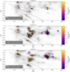 |
Fig. 7 Comparison between radial velocities assigned to clouds with our method (marked with crosses) and those derived from KI spectra and attributed by Ivanova et al. (2021) to dust structures located in the same region of 3D space (marked with circles). We show the results in vertical planes containing the Sun and oriented toward the longitude 1 indicated at the top of the figures. As in Paper I, all data points in the interval [l − 1.25°, l + 1.25°] are treated as if they were contained in the 1 plane. The extinction density map at the given longitude is shown in grayscale. Our points are positioned at the barycenter of the clumps in the considered lines of sight, and the mean velocities are reported via the color bar. Points based on interstellar KI and initially manually located by Ivanova et al. (2021) close to the assigned clouds are kept at the same positions. In blue are the contours of the Fellwalker clumps in the given slice that have an assigned velocity and show the presence product lower than 0.375, and in green are the ones with a presence product of greater than 0.375, while non-assigned clumps are in black. The dotted line marks the b = −28° limit of the CO emission spectral cube. In a given clump, the sampling is every 1.0° in b and 0.125° in l. Empty crosses are used where the Fellwalker clump is only 1 voxel deep, which means it is not possible to calculate a barycenter. |
6 Comparisons with previous results
6.1 Comparisons with neutral potassium absorption data
In Paper I, we describe a nonautomated method of velocity assignment to the dust concentrations appearing in the 3D extinction density maps of the same volume (Ivanova et al. 2021). As briefly mentioned in Sect. 1, constraints on the velocities were based on Doppler shifts of absorption lines in the high-resolution spectra of about 120 target stars distributed in the volume at known distances. Profile fitting of neutral potassium lines provided between one and four velocity components for each star. The synthesis of the velocities, absorption strengths, and distances for the whole set of targets allowed us to assign radial velocities to a series of the structures seen in extinction and located along the lines of sight to the target stars. The average uncertainty on the velocity was on the order of 1.0 to 2.0 km s−1 as a result of calibration uncertainties and profile-fitting simplifications. We note that, due to the limited number of targets, the location of the dust concentration responsible for a given velocity component was rather imprecise, especially in regions of clumpy structures in close proximity to one other.
Figures 7, 8, 9, and 10 show how our automated velocity assignments compare with these independent, nonautomated assignments. The velocities found by Ivanova et al. (2021) are marked with circles in the figures, at the locations manually assigned by the authors. Their positions and velocities are also indexed in Table 3. The color scale used for both types of results on velocities is the same, allowing us to compare their values. Again, we emphasize that these absorption-based results are approximate locations. Because they come from line-of-sight-integrated data, there is some freedom for the location assignment but there are difficulties in regions where there are several maxima of extinction between the available target stars. Moreover, most of the time, the locations for the assigned velocities were displaced from the lines of sight to the target stars in order to avoid overlapping. Finally, our automated method here provides velocities associated with the densest parts of the clouds, while Ivanova et al. (2021) measure velocities along the exact sight lines to the targets, which in general do not cross the densest areas. Nevertheless, despite these limitations, it is possible to visualize the high extinction regions to which they correspond. A look at the series of vertical planes in the figures shows that at locations where nonautomated KI determinations were made, there is general agreement between the two types of results given the uncertainties. This gives us confidence in other assignments in areas where KI results are absent. We also see a few disagreements. A careful look at the results for l = 157.5, 160, and 180° in the Taurus area (r = 130–180 pc) reveals that a few (respectively 1, 2, and 3) circles are drawn with colors indicating low velocities of between −1.5 and +1 km s−1, while there are no corresponding crosses with the same color. While for some of the stars, the absorbing columns are very small and the detection may be uncertain, for others, such as HD 285016 (star 41, v = −1.5 km s−1) and HD 284938 (star 44, v = −1 km s−1), the absorption is clearly defined (see Figs. 10 and 12 of Ivanova et al. 2021). Indeed, the maps suggest the existence of two structures in the main Taurus cloud at a distance of ≃40 pc to each other, and the discrepant circles were all located close to the more distant one. The cloud numbered 52 (see Table 1) in the external part of Taurus at 167 pc and centered at l = 178° is the only one in Taurus to be assigned a low velocity of 2.4 ± 1.0 km s−1 and may correspond to this low velocity detected with the potassium lines, and the more distant part of Taurus. However, in Fig. 10 (top), cloud 52 appears co-located with the higher velocity clouds, it is given a low quality index, and the velocity of 2.4 km s−1 is above the one measured with absorption lines. We believe that the difficulty here resides in the insufficient resolution of the extinction map and the resulting lack of distinction between of the two closer and more distant structures. This problem affects the particularly complex and wide Taurus area. Except for this discrepancy, there are validations for each clump that has values coming from the absorption and a good presence (green contours in Figs. 7, 8, 9 and 10). For clouds with a lower quality index, and apart from the above-mentioned region, most of them are also in rather good agreement.
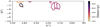 |
Fig. 11 Contours of the clumps in our map outside of the main Taurus region. The map is in Galactic coordinates. |
Mean coordinates and assigned velocity.
6.2 Other comparisons
In Fig. 14 and Tables 4 and 5, we compare our results with those of Zucker et al. (2018) and Galli et al. (2019) for areas in common. As detailed in Sect. 1, Zucker et al. (2018) searched for correspondences between CO emission velocity components and raising steps in cumulative reddening toward known dense structures of Perseus, while Galli et al. (2019) derived the velocities of a number of Taurus clouds based on the velocities of the young stellar objects (YSOs) from clusters embedded in the clouds. Both studies reach a superior degree of precision compared to our present results. In the case of Zucker et al. (2018), the authors used CO data dedicated to the Perseus area that are characterized by very high signal and spectral resolution. In the case of velocities based on YSOs, the authors were able to use the clustering to improve the precision on the local velocity. Despite these differences, it is informative to compare our assignments with both types of results, as they are obtained in a totally independent way. Typical uncertainties are less than or equal to 0.6 km s−1 and on the order of 2 km s−1 for the two works, respectively. Figure 14 shows the locations of the regions with velocities assigned by both studies, superimposed on the projected contours of our extinction structures, all colored according to their average radial velocity. In the case of the Taurus young star clusters of Galli et al. (2019), they are part of the three distinct series of clouds clearly seen in Fig. 9 and located at increasing distances (about 130, 170, and 200 pc). As seen in Tables 4 and 1, there is agreement on distance-velocity associations given uncertainties and internal velocity dispersion within the clouds, for all points except for the clusters G10 (T Tau) and G11 (L1551). These points compare with our extinction regions numbered 15 and 17, respectively. Both are part of a very dense region where our decomposition lacks details and where the window used for the velocity assignment is almost fully filled with adjacent clouds, resulting in presence ratios that are not sufficiently discriminating. For Perseus, the velocities assigned by Zucker et al. (2018) seem to agree − within uncertainties − with those of our clumps 173 and 178 (see Tables 5 and 1). We note the similarity between the velocity decrease with latitude observed here for longitudes of between 155 and 160° and the velocity gradient measured with better precision by Zucker et al. (2018).
7 Conclusions and perspectives
We present a novel technique of automated kinetic tomography of dense molecular clouds. The method is based on 3D dust extinction density maps and CO emission spectra, and the assignment of radial velocities to the clouds is uniquely based on morphological criteria on the one hand, namely the properties of the projected contours of extinction structures, and on the contours associated with CO emission in specific velocity intervals on the other. Individual extinction structures are issued from a Fellwalker discretization of the 3D dust distribution. The method was tested on the set of nearby clouds forming the Taurus, Auriga, Perseus, and California groups. The choice of this particularly complex CO-rich area is motivated by the availability of comparisons with previous, independent results. Application of our novel technique allowed us to assign a velocity to a large fraction of the dust structures issued from Fellwalker (42 from a total of 45). The three remaining structures have direction and distance very similar to neighboring structures with assigned velocities, and they may simply be continuations of those neighbors. We ranked the assignments based on geometrical criteria. Except for a few low-confidence associations, we found good agreement with independent determinations of velocities, regardless of their sources, synthesis of KI absorption towards individual stars, combination of reddening measurements along dense cloud directions and corresponding CO spectra, or YSO clustering in the direction of known molecular clouds.
Our results show that automated kinetic tomography based on morphological criteria and applied to structures extracted from 3D extinction density distributions on the one hand and radio emission data on the other is a realistic objective. They demonstrate the rare occurrence of situations with two or more distinct clouds at different velocities, distributed in distance along the same direction, and with projected contours so similar that disentanglement is precluded. Our results suggest that the application of the method to larger volumes and larger velocity differences between the groups of clouds is feasible. Work is in progress in this direction.
The application of the technique to other volumes of gas and dust will necessitate that we adapt the values of the various parameters entering the algorithm, and in particular the number of velocities treated separately. The optimal choice of these velocities depends on the spatial resolution of the dust map and the number of discrete structures issued from the decomposition of the continuous extinction density distribution, on the spectral resolution of the emission data, on the noise level, and, finally, on the extent of the region of space to be treated. In particular, the Fellwalker decomposition has some arbitrary aspects and other types of decomposition should be attempted. This is beyond the scope of this work, the main aim of which is to validate our new technique. We expect more resolved and more extended 3D extinction maps in the near future because of the continuous production of massive amounts of parallaxes and photometric data from Gaia, as well as data from ground-based surveys. This should allow us to obtain further details about the radio spectral resolution and to take better advantage of it and of more sensitive radio data. Although the application of this technique to large distances and low latitudes – that is, to a large number of clouds with overlapping projections – is expected to be increasingly difficult, it should be facilitated by the fact that the projections of the distant clouds are in general smaller than those of the foreground objects, and as a consequence the contours should be disentangled thanks to the ratios discussed above.
It remains the case that some structures lack velocity assignments, mainly because 3D extinction maps are of limited resolution and are not realistic enough in some areas. This is why it is clear that combining or complementing the present technique – which is solely based on morphology - with more quantitative arguments, greater brightness of emission, greater opacity, and more absorption lines is expected to produce better results and certainly merits further development. In such combinations, the application of the present method would provide a useful firstorder solution for obtaining kinetic tomography. In particular, it could serve as a starting point to the application – region by region – of techniques similar to the one developed by Zucker et al. (2018), which require some preliminary constraints on velocity intervals.
The application to other tracers (HI, CI+) detected in emission is also feasible in principle, and in this case the restriction mask would have to be modified or removed. In the case of HI, the significantly larger width of velocity components associated with the atomic phase would render the analysis significantly more difficult. A preliminary application to CO, and subsequent application to HI with some imposed parameters, may be an approach worth attempting.
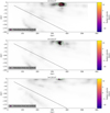 |
Fig. 12 Similar to Fig. 7 but for longitudes of less than 150° featuring clumps with an assigned velocity. |
 |
Fig. 13 Similar to Fig. 7 but for longitudes of less than 150° featuring clumps with an assigned velocity. |
Position and velocities for points coming from Galli et al. (2019).
Position and velocities for areas coming from Zucker et al. (2018).
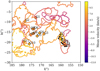 |
Fig. 14 Projection of clump contours, colored according to their assigned mean velocity (right scale). The map is in Galactic coordinates. The results of Zucker et al. (2018) and Galli et al. (2019) are superimposed as markers at their average direction and with the same color scale for their peak-reddening velocities. The areas investigated by Zucker et al. (2018) are designated using a Zx annotation, while the points of Galli et al. (2019) are marked out by aGx. |
Acknowledgements
We are grateful to our referee for their quick reading and thoughtful, constructive comments and criticisms. Q.D. and C.H. acknowledge the CNES Gaia support, with a funding under “identifiant action 6187”. J.-L.V. acknowledges support from the EXPLORE project. EXPLORE has received funding from the European Union’s Horizon 2020 research and innovation programme under grant agreement No 101004214. This work has made use of data from the European Space Agency (ESA) mission Gaia (https://www.cosmos.esa.int/gaia), processed by the Gaia Data Processing and Analysis Consortium (DPAC, https://www.cosmos.esa.int/web/gaia/dpac/consortium). Funding for the DPAC has been provided by national institutions, in particular the institutions participating in the Gaia Multilateral Agreement. This work also makes use of data products from the 2MASS, which is a joint project of the University of Massachusetts and the Infrared Processing and Analysis Center/California Institute of Technology, funded by the National Aeronautics and Space Administration and the National Science Foundation. This research has made use of the SIMBAD database, operated at CDS, Strasbourg, France.
Appendix A Restriction mask
The role of the restriction mask mentioned in section 3.1 is to eliminate from the 3D extinction distribution those volumes whose projections on the sky correspond to no CO emission. It must encompass all the features of the CO map, but our aim here is to avoid overly complex contours. Figure A.1 illustrates three approaches including the selected one. The easiest way would be to integrate the CO data over the full velocity range, to estimate the noise level for this integrated map, and to use it as a threshold value. This leads to a very noisy mask (shown in Fig. A.1:top), and some features, such as the cloud at l = 155° and b = −15°, do not appear clearly. We can go one step further by de-noising the CO map using ROHSA. This has the effect of maintaining isolated pixels with weak intensity in the exclusion process, which correspond to noisy data. However, there is a risk of also eliminating real weak features characterized by a very narrow velocity range. To avoid the loss of such narrow and weak features of the spectrum, we defined a threshold based on the standard deviation of the individual CO spectral cube elements, instead of using the velocity-integrated elements. This method is slightly better, but far from perfect, as shown in Fig. A.1:middle. We finally built a mask based on the output of the Fellwalker algorithm applied to the CO map, after preliminary de-noising by means of ROHSA. We used the same threshold value as the one used in the previous step (see also Part 3.1). The Fellwalker algorithm allows us to identify structures out of the noise. The mask based on the third method is also shown in Fig. 2.
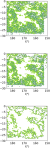 |
Fig. A.1 Restriction masks obtained with different methods.Top: restriction mask obtained by estimating the noise on the velocity-integrated Dame et al. (2001) CO data and keeping the lines where the integrated intensity is above the threshold (0.84K km s−1). Middle: mask obtained after de-noising the CO signal with ROHSA, then keeping all the lines that have a position-position-velocity of at least above the threshold used for Fellwalker, namely 0.20 K. Bottom: mask obtained by applying the Fellwalker algorithm to the post-ROHSA data. This is the mask we used in our search for velocity assignment. |
References
- Berry, D. S. 2015, Astron. Comput., 10, 22 [Google Scholar]
- Dame, T. M., Hartmann, D., & Thaddeus, P. 2001, ApJ, 547, 792 [Google Scholar]
- Galli, P. A. B., Loinard, L., Bouy, H., et al. 2019, A&A, 630, A137 [NASA ADS] [CrossRef] [EDP Sciences] [Google Scholar]
- Green, G. M., Schlafly, E. F., Finkbeiner, D., et al. 2018, MNRAS, 478, 651 [Google Scholar]
- Hottier, C., Babusiaux, C., & Arenou, F. 2021, A&A, 655, A68 [NASA ADS] [CrossRef] [EDP Sciences] [Google Scholar]
- Ivanova, A., Lallement, R., Vergely, J. L., & Hottier, C. 2021, A&A, 652, A22 [NASA ADS] [CrossRef] [EDP Sciences] [Google Scholar]
- Lallement, R., Babusiaux, C., Vergely, J. L., et al. 2019, A&A, 625, A135 [NASA ADS] [CrossRef] [EDP Sciences] [Google Scholar]
- Lallement, R., Vergely, J. L., Babusiaux, C., & Cox, N. L. J. 2022, A&A, 661, A147 [NASA ADS] [CrossRef] [EDP Sciences] [Google Scholar]
- Lewis, J. A., Lada, C. J., & Dame, T. M. 2022, ApJ, 931, 9 [NASA ADS] [CrossRef] [Google Scholar]
- Marchal, A., & Miville-Deschênes, M.-A. 2021, ApJ, 908, 186 [NASA ADS] [CrossRef] [Google Scholar]
- Marchal, A., Miville-Deschênes, M.-A., Orieux, F., et al. 2019, A&A, 626, A101 [NASA ADS] [CrossRef] [EDP Sciences] [Google Scholar]
- Marchal, A., Martin, P. G., & Gong, M. 2021, ApJ, 921, 11 [NASA ADS] [CrossRef] [Google Scholar]
- Peek, J. E. G., Tchernyshyov, K., & Miville-Deschenes, M.-A. 2022, ApJ, 925, 201 [NASA ADS] [CrossRef] [Google Scholar]
- Puspitarini, L., Lallement, R., Babusiaux, C., et al. 2015, A&A, 573, A35 [NASA ADS] [CrossRef] [EDP Sciences] [Google Scholar]
- Tchernyshyov, K., & Peek, J. E. G. 2017, AJ, 153, 8 [Google Scholar]
- Tchernyshyov, K., Peek, J. E. G., & Zasowski, G. 2018, AJ, 156, 248 [NASA ADS] [CrossRef] [Google Scholar]
- Vergely, J. L., Lallement, R., & Cox, N. L. J. 2022, A&A, 664, A174 [NASA ADS] [CrossRef] [EDP Sciences] [Google Scholar]
- Wenger, T. V., Balser, D. S., Anderson, L. D., & Bania, T. M. 2018, ApJ, 856, 52 [Google Scholar]
- Zucker, C., Schlafly, E. F., Speagle, J. S., et al. 2018, ApJ, 869, 83 [NASA ADS] [CrossRef] [Google Scholar]
All Tables
All Figures
|
Fig. 1 Target stars used to build the 3D extinction density map in the Taurus area. The locations of the stars are shown as dots colored according to their extinction (color scale to the right of the figure). White areas correspond to high-opacity central regions within the main dust clouds (extinctions above ≃4 to 5 mag) and mark the subsequent lack of targets with precise distances and photometry due to their faintness. The reconstructed dust distribution will reproduce the clouds but underestimate the corresponding high opacity of the cores. |
| In the text | |
|
Fig. 2 Restriction mask and clump obtained. Top: restriction mask determined from the CO spectra (see Sect. 3.1) and applied to the 3D extinction map before its Fellwalker decomposition step. Masked areas are in black and superimposed on an image of the cumulative extinction integrated between 0 and 1 kpc within the inverted 3D extinction density distribution. The yellow contour corresponds to an integrated CO intensity of 0.11 K.km s−1. The unmasked areas encompass all regions where CO is present,includingareas of very weak intensityclose to the measurement uncertainty level, except very close to the Galactic Plane due to the limited size of the 3D map (see text). Bottom: projection in the same area of the discrete extinction clouds issued from the Fellwalker decomposition. Cloud contours are colored according to their mean distance from the Sun (right scale). |
| In the text | |
|
Fig. 3 Median emission profiles integrated within the projected contours of three clumps, numbered 8, 104, and 114 (black curves), and their fit with a multi-Gaussian function (blue curves). Individual Gaussian components of the function are also detailed in red, orange, green, and gray. The noise level of the profile is indicated by a dashed horizontal line. Clump 114 has a smaller angular size than the two others, which explains its higher noise level. |
| In the text | |
|
Fig. 4 Integrated emission between the velocity bounds of each Gaussian component (central velocity ± the standard deviation) for clump 8 (central velocities 8.8, 11.5, 7.2 and 4.1 km s−1 respectively). The yellow upper limit of the color scale corresponds to the emission level at which the component is considered to be present in the line of sight. The CC clump contours are shown in green and the contours of the neighboring clouds constituting EC are shown in red. |
| In the text | |
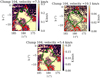 |
Fig. 5 Same as Fig. 4 but for clump 104 (velocities 7.5, 10.1, and 5.4 km s−1). |
| In the text | |
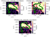 |
Fig. 6 Same as Fig. 4 but for clump 114 (velocities 7.5, 10.1, and 5.4 km s−1). |
| In the text | |
|
Fig. 7 Comparison between radial velocities assigned to clouds with our method (marked with crosses) and those derived from KI spectra and attributed by Ivanova et al. (2021) to dust structures located in the same region of 3D space (marked with circles). We show the results in vertical planes containing the Sun and oriented toward the longitude 1 indicated at the top of the figures. As in Paper I, all data points in the interval [l − 1.25°, l + 1.25°] are treated as if they were contained in the 1 plane. The extinction density map at the given longitude is shown in grayscale. Our points are positioned at the barycenter of the clumps in the considered lines of sight, and the mean velocities are reported via the color bar. Points based on interstellar KI and initially manually located by Ivanova et al. (2021) close to the assigned clouds are kept at the same positions. In blue are the contours of the Fellwalker clumps in the given slice that have an assigned velocity and show the presence product lower than 0.375, and in green are the ones with a presence product of greater than 0.375, while non-assigned clumps are in black. The dotted line marks the b = −28° limit of the CO emission spectral cube. In a given clump, the sampling is every 1.0° in b and 0.125° in l. Empty crosses are used where the Fellwalker clump is only 1 voxel deep, which means it is not possible to calculate a barycenter. |
| In the text | |
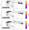 |
Fig. 8 Same as Fig. 7 but for longitudes between 161.25° and 168.75°. |
| In the text | |
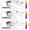 |
Fig. 9 Same as Fig. 7 but for longitudes between 168.75° and 176.25°. |
| In the text | |
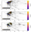 |
Fig. 10 Same as Fig. 7 but for longitudes of between 176.25° and 183.75°. |
| In the text | |
|
Fig. 11 Contours of the clumps in our map outside of the main Taurus region. The map is in Galactic coordinates. |
| In the text | |
|
Fig. 12 Similar to Fig. 7 but for longitudes of less than 150° featuring clumps with an assigned velocity. |
| In the text | |
|
Fig. 13 Similar to Fig. 7 but for longitudes of less than 150° featuring clumps with an assigned velocity. |
| In the text | |
|
Fig. 14 Projection of clump contours, colored according to their assigned mean velocity (right scale). The map is in Galactic coordinates. The results of Zucker et al. (2018) and Galli et al. (2019) are superimposed as markers at their average direction and with the same color scale for their peak-reddening velocities. The areas investigated by Zucker et al. (2018) are designated using a Zx annotation, while the points of Galli et al. (2019) are marked out by aGx. |
| In the text | |
|
Fig. A.1 Restriction masks obtained with different methods.Top: restriction mask obtained by estimating the noise on the velocity-integrated Dame et al. (2001) CO data and keeping the lines where the integrated intensity is above the threshold (0.84K km s−1). Middle: mask obtained after de-noising the CO signal with ROHSA, then keeping all the lines that have a position-position-velocity of at least above the threshold used for Fellwalker, namely 0.20 K. Bottom: mask obtained by applying the Fellwalker algorithm to the post-ROHSA data. This is the mask we used in our search for velocity assignment. |
| In the text | |
Current usage metrics show cumulative count of Article Views (full-text article views including HTML views, PDF and ePub downloads, according to the available data) and Abstracts Views on Vision4Press platform.
Data correspond to usage on the plateform after 2015. The current usage metrics is available 48-96 hours after online publication and is updated daily on week days.
Initial download of the metrics may take a while.