| Issue |
A&A
Volume 630, October 2019
|
|
|---|---|---|
| Article Number | A137 | |
| Number of page(s) | 23 | |
| Section | Galactic structure, stellar clusters and populations | |
| DOI | https://doi.org/10.1051/0004-6361/201935928 | |
| Published online | 07 October 2019 | |
Structure and kinematics of the Taurus star-forming region from Gaia-DR2 and VLBI astrometry⋆
1
Laboratoire d’Astrophysique de Bordeaux, Univ. Bordeaux, CNRS, B18N, Allée Geoffroy Saint-Hilaire, 33615 Pessac, France
e-mail: This email address is being protected from spambots. You need JavaScript enabled to view it.
2
Instituto de Radioastronomía y Astrofísica, Universidad Nacional Autónoma de México, Apartado Postal 3-72, Morelia 58089, Mexico
3
Instituto de Astronomía, Universidad Nacional Autónoma de México, Apartado Postal 70-264, 04510 Ciudad de México, Mexico
4
Depto. de Inteligencia Artificial, UNED, Juan del Rosal, 16, 28040 Madrid, Spain
5
Max Planck Institut für Radioastronomie, Auf dem Hügel 69, 53121 Bonn, Germany
6
Department of Astronomy, University of Massachusetts, Amherst, MA 01003, USA
7
Instituto de Astronomía, Universidad Nacional Autónoma de México, Unidad Académica en Ensenada, Ensenada 22860, Mexico
8
Department of Physics and Astronomy, Western Washington University, 516 High St, Bellingham, WA 98225, USA
Received:
20
May
2019
Accepted:
26
August
2019
Abstract
Aims. We take advantage of the second data release of the Gaia space mission and the state-of-the-art astrometry delivered from very long baseline interferometry observations to revisit the structure and kinematics of the nearby Taurus star-forming region.
Methods. We apply a hierarchical clustering algorithm for partitioning the stars in our sample into groups (i.e., clusters) that are associated with the various molecular clouds of the complex, and derive the distance and spatial velocity of individual stars and their corresponding molecular clouds.
Results. We show that the molecular clouds are located at different distances and confirm the existence of important depth effects in this region reported in previous studies. For example, we find that the L 1495 molecular cloud is located at d = 129.9+0.4−0.3 pc, while the filamentary structure connected to it (in the plane of the sky) is at d = 160.0+1.2−1.2 pc. We report B 215 and L 1558 as the closest (d = 128.5+1.6−1.6 pc) and most remote (d = 198.1+2.5−2.5 pc) substructures of the complex, respectively. The median inter-cloud distance is 25 pc and the relative motion of the subgroups is on the order of a few km s−1. We find no clear evidence for expansion (or contraction) of the Taurus complex, but signs of the potential effects of a global rotation. Finally, we compare the radial velocity of the stars with the velocity of the underlying 13CO molecular gas and report a mean difference of 0.04 ± 0.12 km s−1 (with rms of 0.63 km s−1) confirming that the stars and the gas are tightly coupled.
Key words: open clusters and associations: individual: Taurus / stars: formation / stars: distances / methods: statistical
Full Tables A.1 and A.3 are only available at the CDS via anonymous ftp to cdsarc.u-strasbg.fr (130.79.128.5) or via http://cdsarc.u-strasbg.fr/viz-bin/cat/J/A+A/630/A137
© P. A. B. Galli et al. 2019
 Open Access article, published by EDP Sciences, under the terms of the Creative Commons Attribution License (http://creativecommons.org/licenses/by/4.0), which permits unrestricted use, distribution, and reproduction in any medium, provided the original work is properly cited.
1. Introduction
The Taurus-Auriga star-forming region (or simply Taurus) is one of the most intensively studied regions of low-mass star formation and an ideal laboratory for observing young stellar objects (YSOs) from the most embedded sources at the early stages of evolution (i.e., protostars) to disk-free stars that are actively forming planets (see, e.g., Kenyon et al. 2008). Previous studies suggest that Taurus hosts a few hundred YSOs spread over a large area on the sky of about 15 × 15 deg (Esplin et al. 2014; Esplin & Luhman 2017). The sky-projected spatial distribution shows that the stars are not randomly distributed but clustered in small groups and overdense structures in and around the different star-forming clouds and filaments of the region (Gomez et al. 1993; Joncour et al. 2017, 2018). The morphology and kinematics of these gaseous clouds and filaments have been clearly characterized in recent years based on CO surveys and extinction maps (see, e.g., Ungerechts & Thaddeus 1987; Cambrésy 1999; Dame et al. 2001; Dobashi et al. 2005; Goldsmith et al. 2008), and increasing progress is being made to constrain the three-dimensional structure and stellar kinematics of the individual clouds. However, until recently many studies have been hampered by the lack of accurate data for a significant number of stars, in particular stellar distances and spatial velocities, which could provide us with valuable information about the star formation history in this region.
Distances to individual stars are, in general, derived from trigonometric parallaxes; until recently there were very few parallaxes for Taurus stars. Bertout et al. (1999) used the trigonometric parallaxes of 17 stars from the HIPPARCOS catalog (ESA 1997) and estimated the distances to three groups in this sample,  ,
,  , and
, and  pc, which are roughly associated with the central, northern, and southern clouds of the complex, respectively. The situation did not improve significantly with the first data release of the Gaia space mission (Gaia-DR1; Gaia Collaboration 2016). The Tycho-Gaia Astrometric Solution (TGAS; Lindegren et al. 2016) catalog provided trigonometric parallaxes for only 19 stars in Taurus that are obviously more precise than the HIPPARCOS results for the same stars, but still represent a small fraction of the sample of known members. This sample is restricted to the brightest stars (i.e., G < 12 mag) and the parallaxes were nevertheless affected by systematic errors on the order of 0.3 mas (see Lindegren et al. 2016).
A major effort to determine the distance to individual stars in the Taurus region was successfully undertaken using very long baseline interferometry (VLBI; Lestrade et al. 1999; Loinard et al. 2007; Torres et al. 2007, 2009, 2012). In recent years the Gould’s Belt Distances Survey (GOBELINS; Loinard et al. 2011) has targeted a number of YSOs in nearby star-forming regions to deliver state-of-the-art trigonometric parallaxes and proper motions (see Ortiz-León et al. 2017a,b, 2018; Kounkel et al. 2017). In one paper in this series, Galli et al. (2018) measured the trigonometric parallaxes of 18 stars in Taurus with precision ranging from 0.3% to 5%. The resulting distances suggest that the various molecular clouds of the complex are located at different distances and reveal the existence of significant depth effects in this region. For example, the Lynds 1531 and 1536 molecular clouds (hereafter L 1531 and L 1536) were reported to be the closest (d = 126.6 ± 1.7 pc) and most remote (d = 162.7 ± 0.8 pc) structures of the complex, respectively. The VLBI astrometry combined with published radial velocities yielded a one-dimensional velocity dispersion of about 2–3 km s−1 among the various clouds in Taurus. This is significantly lower than the value of 6 km s−1 used by Bertout & Genova (2006) to derive kinematic distances based on the convergent point method. Such a discrepancy could arise, for example from the internal motions within the complex, indicating that more study is clearly warranted in this regard.
The small number of sources with complete data in the sample (proper motion, parallax, and radial velocity) compared to the number of known members prevented Galli et al. (2018) from investigating in more detail the three-dimensional structure and kinematics of the various subgroups. In this context, the recently published second data release of the Gaia space mission (Gaia-DR2; Gaia Collaboration 2018a) offers a unique opportunity to revisit the previous analysis with a much more significant number of stars and the same level of astrometric precision obtained from VLBI observations. For example, Gaia-DR2 increases the number of Taurus stars with available astrometry by a factor of more than 20 compared to its predecessor Gaia-DR1 including the faintest members at G ≃ 20 mag and having smaller systematic errors on the trigonometric parallaxes of about 0.1 mas on global scales (Luri et al. 2018).
In a recent paper Luhman (2018) used Gaia-DR2 data to refine the census of Taurus stars, to identify new candidates with similar properties of known members, and to determine the shape of the initial mass function (IMF). The revised sample of members shows that the older population of stars (> 10 Myr) which was proposed to be associated with this region in other studies (see, e.g., Kraus et al. 2017; Zhang et al. 2018) has no physical relationship with the Taurus molecular clouds, and the Taurus IMF resembles other star-forming regions (e.g., IC 348 and the Orion Nebula Cluster). We incorporated this updated census of stars in our analysis and we present here our discussion of the structure and kinematics of the region.
This paper is organized as follows. In Sect. 2 we describe the sample of stars used in this study for our analysis and in Sect. 3 we compare the VLBI and Gaia-DR2 astrometry for the stars in common between the two projects in the Taurus region. In Sect. 4 we present our methodology based on hierarchical clustering for partitioning the stars in our sample into different groups with similar properties, for rejecting outliers in the sample, and for defining the subsamples of stars that are associated with the various molecular clouds of the Taurus complex. In Sect. 5 we present our results for the distance and spatial velocity of individual stars and subgroups derived from Bayesian inference using the most precise astrometric and spectroscopic data available to date and the existence of internal motions, expansion, and rotation effects in the complex, and we compare the stellar velocities with the kinematics of the underlying gaseous clouds. Finally, we summarize our results and conclusions in Sect. 6.
2. Sample
To construct our initial sample of Taurus stars, we begin by compiling known YSOs and new candidates associated with this region that have been previously identified in the literature. Several studies in the literature have proposed different lists of Taurus stars (see, e.g., Joncour et al. 2017; Kraus et al. 2017; Zhang et al. 2018; Luhman 2018), but the recent study performed by Luhman (2018) shows that the samples of stars proposed by Kraus et al. (2017) and Zhang et al. (2018) are older (> 10 Myr) and show kinematic properties that are inconsistent with membership in Taurus. We therefore restricted our sample of stars to the lists given by Joncour et al. (2017) and Luhman (2018). We combined the sample of 338 stars from Joncour et al. (2017) with the lists of known members (438 stars) and new candidates (62 stars) given by Luhman (2018). The resulting sample consists of 519 stars after removing the sources in common between the two surveys. Multiple systems are counted as one single source in our sample unless they were resolved in these studies or by the Gaia satellite (as described below).
We proceeded as follows to access the astrometric measurements in Gaia-DR2 for our targets and avoid erroneous cross-identifications. Gaia-DR2 provides cross-matched tables with a number of external catalogs. First, we use the unique source identifier from the 2MASS catalog (Cutri et al. 2003) given in the original tables used to construct our sample and cross-match our list of source identifiers with the TMASS_BEST_NEIGHBOUR table provided by the Gaia archive1. This procedure returns the unique Gaia-DR2 source identifier that corresponds to our target, the number of sources in the 2MASS catalog that match the Gaia source, and the number of Gaia sources that have the same source as best-neighbor. We find a direct one-to-one relationship for most sources in our sample, which confirms that they have been correctly identified. We note that three sources (2MASS J04210934+2750368, 2MASS J04400174+2556292, and 2MASS J05122759+2253492) which were not resolved in previous surveys have more than one counterpart in Gaia-DR2. In such cases, we retain the two components of the system and count them as independent stars. Then, we use the resulting list of Gaia-DR2 identifiers to search our targets in the main catalog table (GAIA_SOURCE) and retrieve the astrometric measurements that will be used in the forthcoming analysis. We repeated this procedure for the 492 stars with known 2MASS identifiers in our sample and searched the remaining sources in Gaia-DR2 using their stellar positions and a search radius of 1″. Doing so, we found proper motions and trigonometric parallaxes for 411 stars from our initial sample.
Radial velocities in Gaia-DR2 are available for only 34 stars in our sample, so we searched the CDS/SIMBAD databases (Wenger et al. 2000) to access more radial velocity measurements. Our search in the literature, which was as exhaustive as possible, was based on Wilson (1953), Hartmann et al. (1986, 1987), Herbig & Bell (1988), Reipurth et al. (1990), Duflot et al. (1995), Mathieu et al. (1997), Wichmann et al. (2000), White & Basri (2003), Muzerolle et al. (2003), Gontcharov (2006), Torres et al. (2006), Kharchenko et al. (2007), Scelsi et al. (2008), Nguyen et al. (2012), and Kraus et al. (2017). In addition, we also used the more recent measurements collected with the Apache Point Observatory Galactic Evolution Experiment (APOGEE) spectrograph (Kounkel et al. 2019). In the case of multiple radial velocity measurements in the literature we took the most precise result as our final estimate. By combining these external sources with Gaia-DR2 we found radial velocities for a total of 248 stars.
Table A.1 lists the 519 stars in our initial sample with the data collected from the literature and the membership status of each star as derived from our forthcoming analysis (see Sect. 4).
3. Gaia-DR2 and VLBI astrometry in Taurus
In a recent study, Galli et al. (2018) derived trigonometric parallaxes and proper motions of 18 YSOs in the Taurus region based on multi-epoch VLBI radio observations as part of the GOBELINS project (see Sect. 1). In the following we exclude V1110 Tau from the discussion because it is more likely to be a foreground field star (see discussion in Sect. 4.10 of Galli et al. 2018) and we count the V1096 Tau A-B binary system as one source. We note that 12 YSOs from their sample are also included in Gaia-DR2. Figures 1 and 2 illustrate the comparison of trigonometric parallaxes and proper motions for the stars in common. The mean difference (Gaia-DR2 minus VLBI) and rms of the trigonometric parallaxes between the two projects are 0.035 ± 0.152 mas and 0.526 mas, respectively. The same comparison in proper motions yields a mean difference of 0.455 ± 0.682 mas yr−1 and −0.382 ± 1.194 mas yr−1, and the rms of 2.410 mas yr−1 and 4.154 mas yr−1, respectively, in right ascension and declination.
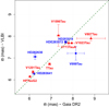 |
Fig. 1. Comparison of the trigonometric parallaxes obtained from the GOBELINS project (Galli et al. 2018) and Gaia-DR2. Blue circles and red triangles indicate the stars that have been modeled as single and binary (multiple) sources for the VLBI astrometry, respectively. The green dashed line indicates perfect correlation between the measurements. |
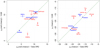 |
Fig. 2. Comparison of the proper motions in right ascension (left panel) and declination (right panel) obtained from the GOBELINS project (Galli et al. 2018) and Gaia-DR2. Blue circles and red triangles indicate the stars that have been modeled as single and binary (multiple) sources for the VLBI astrometry, respectively. The green dashed line indicates perfect correlation between the two measurements. |
Although these numbers provide valuable information for evaluating the consistency (or discrepancy) between VLBI and Gaia-DR2 results, two points are worth mentioning here regarding this comparison. First, the trigonometric parallaxes and proper motions derived from VLBI astrometry for two stars in common with Gaia-DR2 (V999 Tau and HD 282630) have been determined based on a small number of observational epochs. These results are therefore less precise and accurate compared to the other stars in the VLBI sample (see Sect. 4.3 of Galli et al. 2018). Second, the astrometric solutions delivered by Gaia-DR2 assume a model with uniform space motion of the stars so that non-linear motions caused by binarity (and multiplicity) of the source have not been taken into account. Galli et al. (2018) performed a dedicated analysis of the binaries in the VLBI sample and solved for the full orbital motion of these systems with a sufficient number of detections. This explains the discrepancy observed between the two projects for such systems (see also Figs. 1 and 2).
For the reasons discussed above we decided to prioritize the trigonometric parallaxes and proper motions based on VLBI astrometry for both single stars and binaries. In the specific cases of V999 Tau, HD 282630, and the V1096 Tau A-B binary system we prefer to use Gaia-DR2 data because of the small number of observations and the large errors produced in the VLBI solution for these specific sources (see also Sects. 4.1 and 4.3 of Galli et al. 2018). Thus, if we exclude V999 Tau, HD 282630, and V1096 Tau A-B from the comparison, the mean difference and rms of the trigonometric parallaxes between the two projects becomes 0.111 ± 0.115 mas and 0.365 mas, respectively. The former is consistent with the systematic errors of about 0.1 mas that exist in the trigonometric parallaxes of the Gaia-DR2 catalog (see Lindegren et al. 2018). One possibility to explain this discrepancy for the sample of stars under analysis is indeed the different source modeling used in each project. For example, if we remove binaries and multiple systems from this comparison the mean difference between VLBI and Gaia-DR2 results drops to −0.069 ± 0.010 mas (with rms of 0.086 mas).
By combining the recently published Gaia-DR2 catalog with the state-of-the-art VLBI astrometry delivered by the GOBELINS project in the Taurus region, we have a sample of 415 stars with measured trigonometric parallaxes and proper motions. We use the VLBI results obtained by Galli et al. (2018) for 13 stars and Gaia-DR2 data for the remaining 402 stars in this list. The astrometry reference used for each star in this study is indicated in Table A.1.
One important point to mention about Gaia-DR2, which is the main source of data used in our study, is the presence of systematic errors in the catalog. They depend on the position, magnitude, and color of each source, but they are believed to be limited on global scales to 0.1 mas in parallaxes and 0.1 mas yr−1 in proper motion (see, e.g., Luri et al. 2018). We added these numbers in quadrature to the random errors given in the Gaia-DR2 catalog for each star. This procedure is likely to overestimate the parallaxes and proper motion uncertainties for some stars in our sample, but the parameters that result from these observables (e.g., distance and spatial velocity) will take this effect into account when propagating the errors. We also corrected the Gaia-DR2 parallaxes by the zero-point shift of −0.030 mas that is present in the published data, as reported by the Gaia collaboration (see, e.g., Lindegren et al. 2018), although the final impact of this correction in our distances is not significant due to the close proximity of the Taurus star-forming region.
4. Analysis
One of the main objectives of the current study is to compare the properties of the various star-forming clouds in Taurus. In the following we describe our methodology for partitioning the stars in our sample into different groups that roughly define the clouds in the complex. We use the term “cluster” throughout this section to refer to the grouping of stars with similar properties that result from our clustering analysis, and we warn the reader that the terminology used here is not related to the astronomical context (i.e., star clusters).
4.1. Selection criteria
Our sample of YSOs in Taurus compiled from the literature contains 415 stars with measured trigonometric parallaxes and proper motions. However, some of these sources are spread well beyond the molecular clouds of the complex. Thus, we restrict our sample to the general region of the main star-forming clouds in Taurus which roughly spans the following range of Galactic coordinates: 166 ° ≤ l ≤ 180°, −18 ° ≤ b ≤ −6° for the central and northern clouds, and 176 ° ≤ l ≤ 183°, −22 ° ≤ b ≤ −17° for the southernmost clouds of the complex. This reduces our sample to 388 stars.
As explained in the previous section, we are using the astrometric solution from Gaia-DR2 for most sources in this study. The Gaia-DR2 catalog is unprecedented for the quality and quantity of astrometric measurements, but it still contains some spurious solutions that need to be filtered for an optimal usage of the data (see, e.g., Arenou et al. 2018). We proceeded as follows to obtain an astrometrically clean sample of stars. First, we select only the sources with visibility_periods_used > 8, as suggested by Gaia Collaboration (2018b). This removes ten stars from the sample with observations that are not spread out in time and result in poor astrometric solutions. Second, we adopt the renormalized unit weight error (RUWE) of the source as a goodness-of-fit statistic to remove poor astrometric solutions (i.e., RUWE > 1.4)2 This procedure flags 94 sources in our sample, and rejecting them yields the astrometrically clean sample of 284 stars that we use in the forthcoming analysis.
4.2. Clustering analysis
Mode association clustering is a non-parametric statistical approach used for clustering analysis that finds the modes of a kernel-based estimate of the density of points in the input space and groups the data points associated with the same modes into one cluster with arbitrary shape (see Li et al. 2007, for more details). Clustering by mode identification requires only the bandwidth σ of the kernel to be defined. When the bandwidth increases, the density of points becomes smoother and more points are assigned to the same cluster. Thus, a hierarchy of clusters can be constructed in a bottom-up manner by gradually increasing the bandwidth of the kernel functions and treating the modes acquired from the preceding (smaller) bandwidths as new input to be clustered. Hierarchical Mode Association Clustering (HMAC) has the advantage of elucidating the relationship (and hierarchy) among the various clusters in the sample when compared to other commonly used clustering algorithms, for example k-means (MacQueen 1967) and DBSCAN (Ester et al. 1996). It is used in this study to investigate the structure of the Taurus molecular cloud complex and to reveal important clues to the star formation process in this region.
In the forthcoming analysis we use the Modalclust package (Cheng & Ray 2014) which implements the HMAC algorithm in R programming language. We run HMAC from the phmac routine using a number of smoothing levels (i.e., bandwidths) defined as described below, and use the hard.hmac function to access the cluster membership of each star at a given clustering level. We construct our dataset for the clustering analysis with HMAC using only the five astrometric parameters (α, δ, μα cos δ, μδ, ϖ). Many stars in our sample are still lacking radial velocity measurements, thus they will be included only in a subsequent discussion (see Sect. 5) to refine our results. In the first step of our analysis we rescaled the five astrometric parameters so that the resulting distributions have zero mean and unit variance. We obtain the same results using rescaled and non-rescaled parameters, and we therefore decided to work with the non-rescaled astrometry as given in the original sources.
The hierarchical clustering is performed in a bottom-up manner using a sequence of bandwidths σ1 < σ2 < … < σL (in all dimensions) that need to increase by a sufficient amount to drive the merging of the existing clusters at level l with l = 1, 2, …, L, where L is the highest level and merges the full sample into a single cluster. We construct the sequence of bandwidths σl as described below. The smallest bandwidth σ1 that is associated with the lowest level is defined based on the uncertainties of the astrometric parameters used in our analysis. The median errors in the stellar positions (right ascension and declination), proper motions (right ascension and declination), and parallax for the sample of 284 stars are, respectively, 0.093 mas, 0.054 mas, 0.224 mas yr−1, 0.162 mas yr−1, and 0.142 mas. We take the maximum value among the median uncertainties listed before as the bandwidth for the lowest level (i.e., σ1 = 0.224). Then, we proceed as follows for the higher levels (l > 1). We compute the covariance matrix of the clusters at level l (after removing the outliers, see Sect. 4.3), and take the smallest variance observed among all clusters in this level as the bandwidth for the following level. If the new bandwidth does not produce cluster mergers in the next level, we use the second smallest variance and repeat the procedure until at least one merger is produced. This procedure is repeated for all clustering levels until all clusters (and outliers) are clustered into the only existing mode at level L.
Figure 3 shows the resulting hierarchical tree (or dendrogram) obtained with HMAC for the sample of 284 stars. It reveals the existence of 21 clusters at the lowest clustering level which we discuss in more detail in Sect. 4.4 (see cluster membership for each star in Table A.1). We also note the existence of 48 clusters with one single data point, which we consider to be extreme outliers because they exhibit different (unique) properties compared to the other clusters in this level. Table 1 summarizes the results obtained in each clustering level. In Fig. 4 we show that the various clusters obtained from HMAC are indeed associated with different molecular clouds of the Taurus complex. Although the existence of a few additional outliers that could not be identified by the current methodology is still apparent, HMAC has proven to be a useful tool to separate the stars that belong to the several molecular clouds which often exhibit arbitrary shapes and unclear boundaries. The robustness of our clustering results obtained with HMAC is tested in Appendix B based on synthetic data and confirms the results presented in this section.
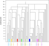 |
Fig. 3. Hierarchical tree (or dendrogram) obtained with HMAC for the sample of 284 stars. The different colors indicate the various clusters at the lowest clustering level of the tree. Outliers that result directly from the HMAC analysis are shown in black. |
Results obtained with HMAC for each clustering level.
4.3. Removing outliers in the individual clusters
HMAC has shown to be able to detect the most extreme outliers in our sample which have been grouped into clusters of one single data point. However, we still note the existence of a more dispersed population of stars in some clusters that clearly extends beyond the limits of the molecular clouds (see, e.g., cluster 7 in Fig. 4). In this section we revise the membership status of these sources and reject potential outliers in the individual clusters. In this context, we use the minimum covariance determinant (MCD; Rousseeuw & Driessen 1999) method that is a robust estimator of multivariate location and scatter efficient in outlier detection.
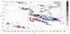 |
Fig. 4. Location of the 284 stars in our sample overlaid on the extinction map from Dobashi et al. (2005) in Galactic coordinates. The different colors represent the sources that belong to the 21 clusters identified at the lowest level of the hierarchical tree obtained with HMAC. Outliers that result directly from the HMAC analysis are shown as black asteriks. The position of the most prominent clouds (Barnard 1927; Lynds 1962) are indicated in the diagram with black triangles. |
Our dataset used for the clustering analysis is stored in an n × p data matrix X = (x1, x2, …, xn)t with xi = (xi1, xi2, …, xip)t for the ith observation, where n is the number of stars in the sample and p is the number of dimensions (variables) used in our analysis (p = 5). The MCD estimator searches the subset of h observations (out of n) that returns the covariance matrix with the lowest determinant. The tolerance ellipse is defined based on the set of p-dimensional points whose MCD-based robust distances
 (1)
(1)
equals  . We denote μ as the MCD estimate of location, Σ as the MCD covariance matrix, and
  as the α-quantile of the
  distribution. Here we use the value of α = 0.975 to construct the tolerance ellipse and identify outliers following the procedure described by Hubert & Debruyne (2010).
We compute the robust distance of the stars in the clusters derived from the HMAC analysis and remove the outliers based on the cutoff threshold  . This procedure is applied to all clusters in our sample with h > p and repeated at each level of the hierarchical tree. The final membership status of each star is given in Table A.1.
4.4. Notes on the individual clusters
In the following we discuss the individual clusters obtained with HMAC at the lowest level of the hierarchical tree. We present the clusters in order of ascending longitude and start with the northernmost clusters, as shown in Fig. 4. Figure 5 shows the proper motions and parallaxes of the stars in the various clusters, and Table A.2 summarizes the cluster properties.
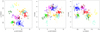 |
Fig. 5. Clustering of the stars in the space of proper motions and parallaxes for the 21 clusters obtained with HMAC (after removing the outliers). |
Cluster 1 is projected towards the northernmost molecular clouds of the complex, L 1517 and L 1519 (see Fig. 6). It is interesting to note the existence of a more dispersed population of stars around these clouds with similar properties of the “on-cloud” population. We confirm that the mean parallax of the more dispersed stars (ϖ = 6.253 ± 0.088 mas) is in good agreement with the mean parallax of the on-cloud stars (ϖ = 6.302 ± 0.046 mas), and both values are consistent with the mean parallax of all stars in the cluster (ϖ = 6.281 ± 0.045 mas, see Table A.2). The proper motions of the two populations are also consistent within 1 mas yr−1 in both components.
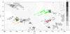 |
Fig. 6. Location of the sources in clusters 1, 2, 3, 4, and 5 overlaid on the extinction map of Dobashi et al. (2005) in Galactic coordinates. The size of the symbols has been rescaled between the minimum and maximum parallaxes observed in each cluster to better distinguish between the closest (big symbols) and most remote (small symbols) members within each cluster. Filled and open symbols indicate, respectively, cluster members and outliers that have been removed in our analysis (see Sect. 4.3). The vectors indicate the stellar proper motions converted to the Galactic reference system (not corrected for solar motion). The position of the most prominent clouds (Barnard 1927; Lynds 1962) is indicated in the diagram with black triangles. |
Clusters 2 and 3 overlap in the same sky region and they are not projected towards any cloud of the complex, as shown in Fig. 6. Their parallaxes differ significantly (see Fig. 5 and Table A.2) which explains the clustering in separate groups.
Cluster 4 is a grouping of seven sources located in the northern part of the Taurus complex. Three of them (V836 Tau, CIDA 8, and CIDA 9B) are projected towards the molecular cloud L 1544 (see Fig. 6), and their mean parallax (ϖ = 5.812 ± 0.095 mas) is consistent with the mean parallax (ϖ = 5.837 ± 0.139 mas) of the more dispersed cluster members (RX J0507.2+2437, CIDA 12 and 2MASS J05080709+2427123).
Cluster 5 contains only two stars (2MASS J05010116+2501413 and 2MASS J05023985+2459337), which are located south of L 1544 (see Fig. 6). Despite the close proximity (in the plane of the sky) to cluster 4, the sources in the two groups exhibit different proper motions (see also Fig. 5), which justifies the clustering in separate groups. Cluster 5 is therefore not associated with any molecular cloud of the complex.
Cluster 6 consists of only three stars (2MASS J04154131+2915078, 2MASS J04154269+2909558, and 2MASS J04154278+2909597) projected towards a molecular cloudlet located northwest of L 1495 (hereafter L 1495 NW). Their parallaxes and proper motions differ significantly from the sources in L 1495 (i.e., cluster 7, see below) despite the close proximity in the plane of the sky (see Figs. 5 and 7). This suggests that L 1495 NW and L 1495 are different structures of the Taurus region.
Cluster 7 is the most populated cluster in our analysis (39 sources) and it is associated with the most prominent molecular cloud of the complex, namely L 1495. The vast majority of stars in this cluster are located in the direction of the dense core B 10 of the cloud and many of the more dispersed sources in the vicinity of L 1495 have been flagged as outliers by the MCD estimator, as illustrated in Fig. 7.
Cluster 8 is associated with the filamentary structure connected (in the plane of the sky) to the central part of the L 1495 molecular cloud. Schmalzl et al. (2010) divided the filament into five clumps (B 211, B 213, B 216, B 217, and B 218) with ranges of 169 ° < l < 172° and −16.2 ° < b < −15.2° (see Fig. 5 of their paper). Most of our sources in this cluster are located between B 213 and B 216 (see Fig. 7), and we detect hints of a gradient in parallaxes along the filament from l = 170.1° (ϖ = 5.900 ± 0.210 mas) to l = 171.0° (ϖ = 6.557 ± 0.162 mas). Figure 5 and Table A.2 show that the parallaxes and proper motions of the sources in the filament and central part of L 1495 (i.e., cluster 7) are significantly different, which confirms them as independent structures. This is also confirmed by the late merging of the two clusters in the hierarchical clustering, as shown in Fig. 3. Interestingly, the stars in the filament exhibit parallaxes and proper motions that are more consistent with the sources in the L 1495 NW cloudlet despite the angular separation of a few degrees on the sky.
Cluster 9 includes two sources (FU Tau A and FF Tau) which are projected towards the B 215 star-forming clump (see Fig. 7). Their parallaxes are still consistent with the sources in L 1495 (cluster 7), but the proper motions are shifted by about 4 mas yr−1 in declination (see also Table A.2).
Clusters 10 has the two stars with the largest proper motions (in right ascension) in the sample (2MASS J04312669+2703188 and 2MASS J04322873+2746117). They are separated by about 1° in the plane of the sky (see Fig. 8) and they are not associated with any star-forming clump. The closest clusters in terms of similarity are clusters 6 and 8. Figure 3 shows that the tree clusters merge at level 11 of the hierarchical tree to form one single group.
Clusters 11 and 12 are spread over 2° in Galactic longitude and each of them contains two stars (see Fig. 8). The two clusters exhibit similar proper motions and parallaxes to the sources in cluster 7 (see Fig. 5). This is confirmed by the early merging of these two clusters with cluster 7 at level 2 of the hierarchical tree to form one single group (see Fig. 3).
Cluster 13 includes only two sources (DL Tau and IT Tau A). Their positions, proper motions, and parallaxes differ from the other clusters in the central region of the complex which justifies the clustering into a different group. IT Tau is projected towards the molecular cloud L 1521 and DL Tau is located in a different cloudlet separated by about 1° in the plane of the sky (see Fig. 8), making it unclear whether this cluster is associated with any cloud of the complex. The small number of sources and their somewhat different sky positions led us to the decision to exclude it from our forthcoming discussion about the properties of the molecular clouds.
Clusters 14 and 15 are collectively discussed because they are both located in the Heiles Cloud 2 and overlap in the plane of the sky (see Fig. 8). The sources in these two clusters are spread over the star-forming clumps L 1527, L 1532, L 1534, and B 220. Their parallax and proper motion values are somewhat different (see Table A.2) and define a different locus in Fig. 5. This indicates the existence of substructures in this cloud that we discuss in our forthcoming analysis using the three-dimensional spatial distribution of the stars (see Sect. 5).
Cluster 16 contains 11 stars spread over the molecular clouds L 1535, L 1529, L 1531, and L 1524 (see Fig. 8). We note that the sources projected towards the various clouds associated with this cluster exhibit similar properties. For example, the sources projected towards the L 1535, L 1529, L 1531, and L 1524 molecular clouds have a mean parallax of ϖ = 7.922 ± 0.105 mas, ϖ = 7.743 ± 0.052 mas, and ϖ = 7.656 ± 0.182 mas, respectively, and they are consistent among themselves. The proper motions of the various sources are consistent within 1–2 mas yr−1. Thus, we discuss their properties collectively under the same group.
Cluster 17 is a grouping of eight sources located north of L 1536 (cluster 18, see below) that is not projected towards any cloud in the complex (see Fig. 8). Despite the close proximity (in the plane of the sky) to the L 1536 molecular cloud, we note that the two clusters define a different locus in the proper motion vector diagram (see Fig. 5).
Cluster 18 is one of the most populated clusters in our sample and it contains 17 stars spread in and around the L 1536 molecular cloud. The most dispersed sources in this cluster have been flagged as outliers by the MCD estimator, as illustrated in Fig. 8.
Cluster 19 hosts four sources (T Tau, IRAS 04187+1927, RX J0422.1+1934, and 2MASS J04221332+1934392) in a small cloud (hereafter the T Tau cloud) in the southern region of the Taurus complex (see Fig. 9). We note in Fig. 5 that the sources in this cluster exhibit the smallest values for the proper motion component in declination among all the clusters in our sample.
Cluster 20 is the second most populated cluster in our analysis. It includes 25 sources that are spread in and around the L 1551 molecular cloud (see Fig. 9). The late merging of clusters 19 and 20 in the hierarchical tree (level 13, see Fig. 3) and the different proper motions (see Fig. 5) suggest that L 1551 and the T Tau cloud are indeed independent structures of the southern region of the Taurus complex.
Cluster 21 includes five sources projected towards the L 1558 molecular cloud (see Fig. 9). As shown in Fig. 5 the sources in this cluster exhibit the smallest parallaxes making it the most distant cluster in our sample (see also discussion in Sect. 5).
4.5. Comparison of our results with those of Luhman (2018)
In a recent study Luhman (2018) divided a sample of Taurus stars into four populations with similar properties of proper motions, parallaxes, and photometry. Two points are worth mentioning here before comparing our results with that study. First, the two studies had distinct objectives which explains the different strategy employed to explore the Gaia-DR2 data in the Taurus region. Luhman (2018) performed an extensive analysis to improve the census of Taurus stars by refining the sample of known members and identifying new candidates. In this context, the sources were not filtered (as done in the present study) to minimize as much as possible the rejection of potential members of the Taurus region. On the other hand, we decided to apply the RUWE selection criterion in the present study, which is a more conservative approach to filter the stars in the sample. This procedure is likely to remove some bona fide members of the Taurus region, but at the same time it minimizes the number of stars with discrepant measurements in the sample due to a poor fit of the Gaia-DR2 astrometric solution or to non-membership. This was made necessary to derive more accurate distances and spatial velocities for the subgroups, as we discuss in more detail in Sect. 5. Second, the methodology used by Luhman (2018) to identify the four populations of stars is based on a manual selection of the sources with similar properties rather than a clustering algorithm. For these reasons, the number of sources and the subgroups themselves identified in the two studies differ from each other, and the comparison between the two solutions is not straightforward. We proceeded as follows to compare the results given by the two studies.
To begin with, we cross-matched our sample of cluster members with the list of stars from Luhman (2018). Figure 10 shows the distribution of Taurus stars in the four populations classified by Luhman (2018) among the various clusters obtained in our clustering analysis with HMAC. We note that the HMAC clusters obtained in our analysis group only stars from one of the four populations discussed by Luhman (2018) (i.e., we do not see a mix of populations in the various clusters). The clusters derived from the HMAC analysis that contain only a subset of the sample of stars given by Luhman (2018), due to the different selection criteria used to filter the Gaia-DR2 sources in each study, as explained before.
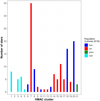 |
Fig. 10. Comparison of the HMAC clustering results obtained in this study with the four populations of Taurus stars (blue, red, green, and cyan) identified by Luhman (2018) from the sample of known Taurus members (Table 1 of that paper). The bar chart indicates the number of stars of each population that are in common with the HMAC clusters. |
Another interesting point to mention is that the four populations of Luhman (2018) are closely related to the HMAC clustering results that we obtained at level 12 of the hierarchical tree (see Fig. 3), as explained below. At this level we have six groups of clusters that include all 21 clusters discussed in Sect. 4.4 (see also Table 1). We label them as follows (from the left to right in Fig. 3): Group A (includes clusters 6, 8, 10, 13, and 18), Group B (includes cluster 20), Group C (includes clusters 1, 2, 3, 4, and 5), Group D (includes cluster 19), Group E (includes cluster 21), and Group F (includes clusters 7, 9, 11, 12, 14, 15, 16, and 17). We note from Fig. 10 that groups A, B and groups D, F correspond to the blue and red populations, respectively. The position of the stars was not used by Luhman (2018) to define the various populations, which explains why the red and blue populations are separated into several groups in the HMAC analysis. Group C represents the cyan population (i.e., the northern clouds) and Group E is associated with the green population.
We note that 51 stars from the sample of 62 new candidate members given in Table 6 of Luhman (2018) have been retained for the clustering analysis after applying the selection criteria described in Sect. 4.1. Twenty-six of them were selected in our analysis and assigned to clusters 1, 2, 3, 5, 7, 10, 11, 12, 17, 20, and 21. In particular, we note that cluster 2 is formed exclusively by new candidate members, which explains in Figure 10 the absence of known Taurus members of the four populations identified by Luhman (2018). In addition, we find 16 stars in the sample of Joncour et al. (2017) that are not included in the list of known members given by Luhman (2018). Only five of them satisfy our selection criteria described in Sect. 4.1, and all of them have been identified as outliers in the HMAC clustering analysis. Table A.1 lists the membership status of each star in our sample given by Joncour et al. (2017) and Luhman (2018) compared to the results obtained in this study.
Thus, we conclude that our methodology based on the HMAC analysis is able to recover the four populations of Taurus stars that were previously identified by Luhman (2018), and that the two studies return consistent results with respect to the clustering of the stars in several substructures across the Taurus complex.
5. Discussion
5.1. Distance and spatial velocity of Taurus stars
In this section we convert the observables used in our clustering analysis (positions, proper motions, and parallaxes) into distances, three-dimensional positions, and spatial velocities to discuss the properties of the stars projected against the various molecular clouds in this region. The forthcoming discussion will be restricted to the 13 clusters listed in Table A.2 that are associated with a molecular cloud of the complex, and hereafter we use the molecular cloud identifiers when refering to the individual clusters rather than the cluster numbering from the HMAC terminology.
First, we convert the trigonometric parallaxes and proper motions of individual stars into distances and two-dimensional tangential velocities using Bayesian inference and following the online tutorials available in the Gaia archive (see Luri et al. 2018). This procedure uses an exponentially decreasing space density prior for the distance with length scale L = 1.35 kpc (Bailer-Jones 2015; Astraatmadja & Bailer-Jones 2016) and a beta function for the prior over speed3. This methodology takes the full covariance matrix of the observables into account to estimate our uncertainties on the final distances and tangential velocities of the stars. Then we use the resulting distances to compute the three-dimensional position XYZ of the stars in a reference system that has its origin at the Sun, where X points to the Galactic center, Y points in the direction of Galactic rotation, and Z points to the Galactic north pole to form a right-handed system.
Second, we combine the resulting two-dimensional tangential velocities with the radial velocities collected from the literature (see Sect. 2) to derive the UVW spatial velocity of the stars in the same reference system as described above and following the transformation outlined by Johnson & Soderblom (1987). We note that 102 stars among those that were confirmed as cluster members in our previous analysis have published radial velocity measurements in the literature. Figure 11 shows the distribution of radial velocities in our sample. We flag the radial velocities for ten stars as outliers based on the interquartile range (IQR) criterium. These measurements lie over 1.5 * IQR below the first quartile (Q1) or above the third quartile (Q3) of the distribution, and in many cases they are likely to be affected by binarity. Thus, we discard the radial velocities of LkCa 1, Anon 1, XEST 20-066, LkCa 3 (V1098 Tau), Hubble 4 (V1023 Tau), MHO 5, HD 28867, DQ Tau, 2MASS J04482128+2927120, and AB Aur when computing the UVW spatial velocities (but we still retain them as cluster members in the forthcoming discussion based on our previous results from Sect. 4).
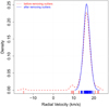 |
Fig. 11. Kernel density estimate (for a kernel bandwidth of 1 km s−1) of the distribution of radial velocity measurements collected from the literature for 102 stars in the sample of cluster members obtained in our clustering analysis with HMAC. The tick marks in the horizontal axis indicate the individual measurements of each star. |
Table A.3 lists the individual distances, three-dimensional positions and spatial velocities for the 174 stars that were confirmed as cluster members (i.e., Member = 1 in Table A.1). We also provide in this table the spatial velocities uvw corrected for the velocity of the Sun relative to the local standard of rest (LSR) using the solar motion of  km s−1 from Schönrich et al. (2010). The formal uncertainties on the distances and spatial velocities provided in this paper are computed from the 16% and 84% quantiles of the corresponding distributions, which roughly provide us with a 1σ standard deviation. Although recent studies based on Bayesian inference (e.g., Bailer-Jones 2015) recommend using a 90% confidence interval (e.g., 5% and 95% quantiles) we decided to proceed as explained above to better compare our results with previous studies that only present the 1σ uncertainty on their results.
We provide in Tables 2 and 3 the distance estimate and the mean spatial velocity of the stars projected towards the molecular clouds represented in our sample. The Bayesian distance for each cloud is computed from the individual parallaxes and their uncertainties based on the online tutorials for inference of cluster distance available in the Gaia archive (see also Luri et al. 2018) and using the same prior over the distance as before. We also list the distances obtained by the more common approach of simply inverting the mean parallax of each molecular cloud. In the latter case it is important to take into account the possible systematic errors in the Gaia-DR2 parallaxes that largely dominate our sample. Although we have already included the systematic errors of 0.1 mas in the uncertainties of Gaia-DR2 parallaxes (as described in Sect. 3), this effect is still present in the mean parallaxes listed in Table A.2 in the sense that averaging the individual parallaxes of cloud members will not reduce the final uncertainties below the 0.1 mas level. We note that the uncertainties on the mean parallaxes given in Table A.2 are much smaller than the the systematic error of 0.1 mas for most clusters (i.e., molecular clouds) in our sample. In these cases we used 0.1 mas as the uncertainty for the mean parallax to estimate the (asymmetric) uncertainties in the distances derived from the inversion method.
Distance of the Taurus molecular clouds.
Spatial velocity of the Taurus molecular clouds.
Figure 12 shows the posterior probability density function obtained for each sample of stars associated with a molecular cloud together with the distance estimates given in Table 2. Interestingly, we note that the posterior probability distribution of the various clouds exhibit somewhat different shapes. For example, L 1495, the most populated cloud in the sample, has a very narrow distribution (e.g., compared with L 1495 NW), which indeed gives the most precise distance estimate in our analysis. Here we report the Bayesian estimates given in Table 2 as our final results for the distance, because this methodology allows for a proper handling of the uncertainties in our data.
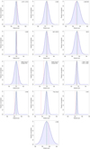 |
Fig. 12. Posterior probability density function of the distance to the various molecular clouds of the Taurus complex. The solid and dashed lines indicate, respectively, the distances obtained from the Bayesian approach (see Sect. 5) and by inverting the mean parallax. |
Our results show that the complex of clouds formed by L 1535, L 1529, L 1531, L 1524 and the B 215 clump are the closest structures to the Sun in the Taurus region ( and
and  pc, respectively). This is consistent with the distance of
  pc obtained previously by Galli et al. (2018) for L 1531 based on the VLBI trigonometric parallax of V807 Tau. The GOBELINS survey in Taurus targeted the central and southern clouds of the complex, so Galli et al. (2018) presented L 1536 as the farthest cloud in the region based on the VLBI parallax of HP Tau G2
  . This distance estimate is in very good agreement with the result of
  pc that we derive in this study for L 1536, but our current analysis in this paper suggests that L 1558
  should hereafter be considered as the most remote molecular cloud in Taurus. In general, we see a good agreement between the results reported in the two studies. The only exception is L 1519 for which Galli et al. (2018) used the Gaia-DR1 parallaxes of three stars and the VLBI parallax of HD 282630 (see discussion of this source in Sect. 3) to estimate the distance to the cloud. The reported distance of
  pc is not consistent with the new result that we derive in this paper using the more accurate and precise Gaia-DR2 parallaxes. The molecular cloud L 1513 listed in Table 10 of that study is not discussed here, because the only source projected towards this cloud (namely UY Aur) was flagged as a potential outlier in our clustering analysis presented in Sect. 4.
5.2. Internal motions, expansion, and rotation
In the following we investigate the internal and relative motions of the stars projected towards the various molecular clouds in the complex. Figure 13 shows the spatial velocity of the stars projected onto the XZ, YZ, and ZX planes after correcting for the solar motion. The stellar motions appear less organized when we remove the velocity of the Sun relative to the LSR, but a bulk motion for the various clouds in the complex is still apparent, as illustrated in Fig. 13. It is interesting to note that the peculiar velocities of the stars projected onto the XY, YZ, and ZX planes reveal the existence of two groups of molecular clouds with velocity vectors pointing towards different directions. One of these groups is formed by L 1495, L 1535, L 1529, L 1531, L 1524, B 215, and Heiles Cloud 2 where the velocity vectors point towards the bottom left corner of the ZX plane, for example. Not surprisingly, these clouds (i.e., clusters) are clustered under the same group in the HMAC hierarchical tree at level 12 (see Fig. 3). This suggests a potentially different formation episode for the various clouds in the complex. Interestingly, this effect is also apparent in the three-dimensional space of velocities (see Fig. 14). The Taurus subgroups listed above exhibit W velocities that are lower by about 2–3 km s−1 compared to the stars in L 1551, L 1536, B 213, and B 216, among others, whose velocity vectors point towards a different direction.
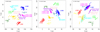 |
Fig. 13. Peculiar velocity of the stars in the various clouds of the Taurus complex projected onto the XY, YZ, and ZX planes. |
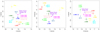 |
Fig. 14. Mean spatial velocity of the stars projected towards the various molecular clouds of the Taurus complex. |
We present in Table 4 the relative motion of the various clouds in the complex. The T Tau cloud is not included in this discussion to avoid a biased result based on only one source with measured radial velocity. The relative motion among the various clouds range from about 1 to 5 km s−1. The highest value that we observe (5.4 ± 0.5 km s−1) occurs between L 1551 and the B 215 clump. The relative motion between the northernmost cloud (i.e., L 1517 and L 1519) and the southernmost cloud (i.e., L 1551) is only 3.2 ± 0.5 km s−1. We measure a significant relative bulk motion of 4.3 ± 0.2 km s−1 between the core of L 1495 and its filament (i.e., B 213 and B 216) confirming that they are indeed independent structures. It is also interesting to note that they exhibit diverging motions in the Z direction (see also Fig. 13). In addition, we also measure a significant non-zero relative motion of Δv = −1.5 ± 0.3 km s−1 in the v component of the peculiar velocity of the stars in the two subgroups of the Heiles Cloud 2 (i.e., clusters 14 and 15), which justifies our decision to discuss them separately throughout this paper. The high values that we find here for the relative motions between some clouds of the complex (see also Luhman 2018) are consistent with the velocity difference among Taurus subgroups reported in the past by Jones & Herbig (1979) and the velocity dispersion of 6 km s−1 used by Bertout & Genova (2006) in the convergent point search method under the assumption that all stars (independent of the molecular cloud to which they belong) are comoving.
Relative space motion among the various clouds of the Taurus complex.
Let us now assess the quantitative importance of random and organized motions within the complex. We investigate the potential expansion and rotation effects in the Taurus region following the procedure described by Rivera et al. (2015). First, we compute the unit position vector  for each star that represents the distance of a given star with respect to the center of the corresponding molecular cloud to which it belongs. Second, we compute the velocity δv* of each star relative to its molecular cloud. The dot product between the two quantities (
 ) is large and positive (negative) if the group is undergoing expansion (contraction). Analogously, the cross product (
 ) stands as a proxy for the angular momentum of the group and it is large (small) in the case of significant (negligible) rotation effects. We compute the dot and cross product for all stars in our sample with respect to the molecular clouds to which they belong and take the mean of the resulting values as a proxy for the expansion (contraction) and rotation velocities of each group. We run these calculations for all molecular clouds with a minimum of three representative stars with known spatial velocities (i.e., with measured radial velocities). The results of our analysis are presented in Table 5. We note that the resulting quantities are consistent with zero (within 5σ of the corresponding uncertainties) suggesting that the expansion and rotation effects in the individual molecular clouds are negligible.
Results for the expansion and rotation velocity of each molecular cloud and the entire complex.
We repeat the same experiment as described above but using the full sample of cluster members with measured radial velocities (92 stars, see Sect. 5.1) to detect large-scale expansion and rotation effects in the Taurus complex. The resulting expansion (contraction) velocity of 0.0 ± 0.1 km s−1 for the entire complex is consistent with zero. This implies that the internal motions in the radial direction of the complex are dominated by random motions rather than an organized expansion or contraction pattern. On the other hand, the non-zero rotational velocity that we derive here ( km s−1, see Table 5) suggests the existence of possible rotation effects in the Taurus complex as a whole. The rotation rate that we derive is nevertheless lower than the result of vrot ≃ 2 km s−1 obtained previously by Rivera et al. (2015) using a sample of only seven stars with VLBI astrometry. However, it is important to mention that this number is still smaller than the observed three-dimensional velocity dispersion of the stars in our sample (
 km s−1, see Table 2). This value suggests that the rotation contributes significantly to the velocity dispersion, but there is also an important contribution from random motions within the complex.
The relative distances between the Taurus subgroups range from about 4 to 50 pc with a median inter-cloud distance of 25 pc (see Table 4). The crossing time between the various subgroups in this region is on the order of several Myr. For example, if we assume a common origin and birthplace for L 1495 and L 1544, a timescale of about 20 Myr is necessary to explain their present-day positions given their relative distance of 50.9 ± 2.1 pc and bulk motion of 2.3 ± 0.4 km s−1. This number greatly exceeds the median age of Taurus stars (∼5 Myr, see, e.g., Bertout et al. 2007).
5.3. Stellar and molecular gas kinematics
In this section we compare the radial velocities of the stars in our sample with the kinematics of the underlying gaseous clouds. We used the large-scale survey of the Taurus molecular clouds in 12CO and 13CO performed by Goldsmith et al. (2008) using the Five College Radio Astronomy Observatory (FCRAO) telescope. The northernmost and southernmost clouds are not included in the surveyed region, so the analysis is restricted to the molecular clouds in the central region of the Taurus complex that fall into the FCRAO maps.
We proceeded as follows to compare the stellar velocities with the kinematics of the molecular gas. First, we convert the (heliocentric) radial velocities of the stars collected from the literature to the LSR. For consistency with our FCRAO data, we deduce the velocity of the Sun with respect to the LSR computed from the solar apex of (α⊙, δ⊙)=(271 ° ,30 ° ) and V⊙ = 20 km s−1 (see Jackson et al. 2006) rather than the solar motion used in Sect. 5.1. The corrected radial velocities of individual stars are listed in Table A.3. Second, we extract the 12CO and 13CO spectra from the FCRAO maps at the position of each star in our sample in a velocity interval from −2 to 14 km s−1 which conservatively includes the range of observed velocities (with respect to the LSR) in Taurus (see, e.g., Fig. 12 of Goldsmith et al. 2008). Then, we compute the centroid velocity and estimate its uncertainty from the rms of the spectrum as described by Dickman & Kleiner (1985).
Two points are worth mentioning here before comparing the stellar radial velocities with the CO velocity. First, the fraction of binaries and multiple systems in Taurus is high (see, e.g., Leinert et al. 1993; Duchêne 1999) and a complete census of these systems with their properties (e.g., orbital period, angular separation, and mass ratio) is still lacking in the literature. We reject all known binaries and multiple systems for the current analysis (many of them have been flagged by Joncour et al. 2017) to avoid comparing the velocity of the gas with a radial velocity measurement that is variable in time. Second, a visual inspection of the extracted spectra for the 12CO molecule reveals that the emission often exhibits complex structures and self-absorbed spectral profiles (see also Urquhart et al. 2007) making it difficult to compute a velocity centroid in such cases. Although the 12CO molecule is more abundant than its isotopolog 13CO, the latter is more optically thin giving access to the full column density that produces the emission (see, e.g., Cormier et al. 2018) and these absorption features are less common in our spectra. We therefore decided to work with the 13CO emission to determine the velocity of the molecular gas along the line of sight. Another interesting feature that we observe in some of our spectra is the existence of multiple (overlapping) components for the velocity of the gas as reported previously by Hacar et al. (2013). It is possible in principle to compare the stellar radial velocities with the closest component of the gas velocity, but we decided to discard these spectra from our analysis to avoid a biased correlation between the two velocities.
Table 6 lists the individual measurements for the velocity of the stars and the 13CO molecular gas used in our comparison. This analysis is restricted to 28 stars in our sample that satisfy the conditions described above. We note that three stars (CW Tau, 2MASS J04213459+2701388, and 2MASS J04414825+2534304) have radial velocities that differ by more than 1 km s−1 with respect to the 13CO molecular gas velocity. One possibility to explain the different velocities for these sources is the existence of undetected binaries because their proper motions and parallaxes are consistent with membership in the corresponding clouds (as discussed in Sect. 4). In particular, we found three heliocentric radial velocity measurements in the literature for CW Tau: 14.5 ± 2.0 km s−1 (Hartmann et al. 1986; Herbig & Bell 1988), 13.60 ± 0.10 km s−1 (Nguyen et al. 2012), and 16.39 ± 0.42 km s−1 (Kounkel et al. 2019). As explained in Sect. 2, we used the most precise measurement throughout our analysis. The difference between the radial velocity of CW Tau and the 13CO molecular gas would still be at the 1 km s−1 level if, for example, we used the most recent measurement of Vr = 16.39 ± 0.42 km s−1 in our comparison. In the case of 2MASS J04213459+2701388 and 2MASS J04414825+2534304 we found only one radial velocity measurement in the literature.
Comparison of the velocity of the stars and the 13CO molecular gas.
As illustrated in Fig. 15 the correlation between the radial velocity of the stars and the velocity of the 13CO molecular gas along the line of sight is clearly evident. Here, we report a mean difference between the two velocities of 0.04 ± 0.12 km s−1 (in the sense stars minus gas) and rms of 0.63 km s−1. Previous studies in this region performed by Herbig (1977) and Hartmann et al. (1986) reported a mean difference of 0.4 ± 0.5 km s−1 (with rms of 3.9 km s−1) and 0.2 ± 0.4 km s−1 (with rms of 1.7 km s−1), respectively. Our results obtained in this paper reveal that the stars and the gas are even more tightly coupled than previously thought. One reason to explain this result comes from the more precise and accurate radial velocity measurements available to date that have been incorporated in our analysis. In addition, it should also be noted that the sample of Taurus stars used in each study is not the same.
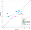 |
Fig. 15. Comparison of the radial velocity of the stars (with respect to the LSR) with the centroid velocity of the 13CO emission extracted from the FCRAO maps at the position of each star. The black dashed line indicates a perfect correlation between the two measurements, and the colors respresent the various molecular clouds to which the stars belong. |
Our results in this section are consistent with the stars being at the same velocity of the neighboring molecular gas. This finding confirms that the stars in our sample are indeed associated with the various substructures of the complex, and supports our results for the existence of multiple populations, significant depth effects, and internal motions in the Taurus region.
6. Conclusions
We used in this study the best astrometry available to date by combining Gaia-DR2 data with the VLBI results delivered by the GOBELINS project to investigate the three-dimensional structure and kinematics of the Taurus star-forming region. Both projects return consistent results for the targets in common and complement each other in this region of the sky.
We applied a hierarchical clustering algorithm for partitioning the stars in our sample into groups with similar properties based on the stellar positions, proper motions, and parallaxes. Our methodology allowed us to identify the various substructures of the Taurus region and discuss their relationship (i.e., hierarchy). We found 21 clusters in our sample at the lowest level of the hierarchical tree and a number of outliers that exhibit discrepant properties. Thirteen of these clusters are associated with one molecular cloud of the Taurus complex and have been used to derive the distance and spatial velocity of the corresponding clouds providing the most complete and precise scenario of the six-dimensional structure of this region.
We confirmed the existence of significant depth effects along the line of sight. The median inter-cloud distance among the various subgroups of the Taurus region is about 25 pc. We report B 215 and L 1558 as the closest  and most remote
  substructures of the complex, respectively. In addition, we show that the core of the most prominent molecular cloud of the complex L 1495 and the filament connected to it in the plane of the sky are located at significantly different distances (
 pc and
  pc, respectively) and diverge from each other in the velocity space.
In a subsequent analysis, we computed the spatial velocities of the stars and the relative bulk motion among the various clouds. The highest values that we derive for the relative motion among the various substructures occur between the B 215 clump in the central region of the complex with the northernmost and southernmost clouds (L 1517, L 1519 and L 1551, respectively) and they reach about 5 km s−1. The one-dimensional velocity dispersion that we obtain from the full sample of Taurus stars with known spatial velocities is on the order of 2 km s−1. In addition, we have also investigated the existence of expansion, contraction, and rotation effects. We concluded that these effects are too small (if present at all) in the individual molecular clouds represented in our sample of stars. We do not detect any significant expansion pattern for the Taurus complex as a whole, but we find evidence of potential rotation effects that will require further investigation with different methodologies.
Finally, we compared the radial velocity of the stars in our sample with the velocity of the underlying gaseous clouds derived from the emission of the 13CO molecular gas, and showed that they are consistent among themselves. We find a mean difference of 0.04 ± 0.12 km s−1 (with rms of 0.63 km s−1), which suggests that the stars are indeed following the velocity pattern of the gas in this region.
See technical note GAIA-C3-TN-LU-LL-124-01 for more details.
See also GAIA-C8-TN-LU-MPIA-CBJ-081 for more details.
Acknowledgments
We thank Alvaro Hacar, Estelle Moraux, and Isabelle Joncour for helpful discussions that improved the manuscript. This research has received funding from the European Research Council (ERC) under the European Union’s Horizon 2020 research and innovation program (grant agreement No. 682903, P.I. H. Bouy), and from the French State in the framework of the “Investments for the future” Program, IdEx Bordeaux, reference ANR-10-IDEX-03-02. L. L. acknowledges the financial support from PAPIIT-UNAM project IN112417, and CONACyT. G. N. O.-L. acknowledges support from the von Humboldt Stiftung. This research has made use of the SIMBAD database, operated at CDS, Strasbourg, France. This work has made use of data from the European Space Agency (ESA) mission Gaia (https://www.cosmos.esa.int/gaia), processed by the Gaia Data Processing and Analysis Consortium (DPAC, https://www.cosmos.esa.int/web/gaia/dpac/consortium). Funding for the DPAC has been provided by national institutions, in particular the institutions participating in the Gaia Multilateral Agreement.
References
- Arenou, F., Luri, X., Babusiaux, C., et al. 2018, A&A, 616, A17 [Google Scholar]
- Astraatmadja, T. L., & Bailer-Jones, C. A. L. 2016, ApJ, 832, 137 [NASA ADS] [CrossRef] [Google Scholar]
- Bailer-Jones, C. A. L. 2015, PASP, 127, 994 [NASA ADS] [CrossRef] [Google Scholar]
- Barnard, E. E. 1927, VizieR On-line Data Catalog: VII/220A [Google Scholar]
- Bertout, C., & Genova, F. 2006, A&A, 460, 499 [NASA ADS] [CrossRef] [EDP Sciences] [Google Scholar]
- Bertout, C., Robichon, N., & Arenou, F. 1999, A&A, 352, 574 [NASA ADS] [Google Scholar]
- Bertout, C., Siess, L., & Cabrit, S. 2007, A&A, 473, L21 [NASA ADS] [CrossRef] [EDP Sciences] [Google Scholar]
- Cambrésy, L. 1999, A&A, 345, 965 [NASA ADS] [Google Scholar]
- Cheng, Y., & Ray, S. 2014, Open J. Stat., 4, 826 [CrossRef] [Google Scholar]
- Cormier, D., Bigiel, F., Jiménez-Donaire, M. J., et al. 2018, MNRAS, 475, 3909 [NASA ADS] [CrossRef] [Google Scholar]
- Cutri, R. M., Skrutskie, M. F., van Dyk, S., et al. 2003, 2MASS All Sky Catalog of Point Sources [Google Scholar]
- Dame, T. M., Hartmann, D., & Thaddeus, P. 2001, ApJ, 547, 792 [NASA ADS] [CrossRef] [Google Scholar]
- Dickman, R. L., & Kleiner, S. C. 1985, ApJ, 295, 479 [NASA ADS] [CrossRef] [Google Scholar]
- Dobashi, K., Uehara, H., Kandori, R., et al. 2005, PASJ, 57, S1 [NASA ADS] [CrossRef] [Google Scholar]
- Duchêne, G. 1999, A&A, 341, 547 [NASA ADS] [Google Scholar]
- Duflot, M., Figon, P., & Meyssonnier, N. 1995, A&AS, 114, 269 [Google Scholar]
- ESA 1997, ESA SP, 1200 [Google Scholar]
- Esplin, T. L., & Luhman, K. L. 2017, AJ, 154, 134 [NASA ADS] [CrossRef] [Google Scholar]
- Esplin, T. L., Luhman, K. L., & Mamajek, E. E. 2014, ApJ, 784, 126 [NASA ADS] [CrossRef] [Google Scholar]
- Ester, M., Kriegel, H. P., Sander, J., & Xu, X. 1996, A Density-based Algorithm for Discovering Clusters in Large Spatial Databases with Noise (AAAI Press), 226 [Google Scholar]
- Gaia Collaboration (Brown, A. G. A., et al.) 2016, A&A, 595, A2 [NASA ADS] [CrossRef] [EDP Sciences] [Google Scholar]
- Gaia Collaboration (Brown, A. G. A., et al.) 2018a, A&A, 616, A1 [NASA ADS] [CrossRef] [EDP Sciences] [Google Scholar]
- Gaia Collaboration (Babusiaux, C., et al.) 2018b, A&A, 616, A10 [NASA ADS] [CrossRef] [EDP Sciences] [Google Scholar]
- Galli, P. A. B., Loinard, L., Ortiz-Léon, G. N., et al. 2018, ApJ, 859, 33 [NASA ADS] [CrossRef] [Google Scholar]
- Goldsmith, P. F., Heyer, M., Narayanan, G., et al. 2008, ApJ, 680, 428 [NASA ADS] [CrossRef] [Google Scholar]
- Gomez, M., Hartmann, L., Kenyon, S. J., & Hewett, R. 1993, AJ, 105, 1927 [NASA ADS] [CrossRef] [Google Scholar]
- Gontcharov, G. A. 2006, Astron. Lett., 32, 759 [NASA ADS] [CrossRef] [Google Scholar]
- Hacar, A., Tafalla, M., Kauffmann, J., & Kovács, A. 2013, A&A, 554, A55 [NASA ADS] [CrossRef] [EDP Sciences] [Google Scholar]
- Hartmann, L., Hewett, R., Stahler, S., & Mathieu, R. D. 1986, ApJ, 309, 275 [NASA ADS] [CrossRef] [Google Scholar]
- Hartmann, L. W., Soderblom, D. R., & Stauffer, J. R. 1987, AJ, 93, 907 [NASA ADS] [CrossRef] [Google Scholar]
- Herbig, G. H. 1977, ApJ, 214, 747 [NASA ADS] [CrossRef] [Google Scholar]
- Herbig, G. H., & Bell, K. R. 1988, Third Catalog of Emission-Line Stars of the Orion Population, 3 [Google Scholar]
- Hubert, M., & Debruyne, M. 2010, Wiley Interdiscip. Rev.: Comput. Stat., 2, 36 [CrossRef] [Google Scholar]
- Jackson, J. M., Rathborne, J. M., Shah, R. Y., et al. 2006, ApJS, 163, 145 [NASA ADS] [CrossRef] [Google Scholar]
- Johnson, D. R. H., & Soderblom, D. R. 1987, AJ, 93, 864 [NASA ADS] [CrossRef] [Google Scholar]
- Joncour, I., Duchêne, G., & Moraux, E. 2017, A&A, 599, A14 [NASA ADS] [CrossRef] [EDP Sciences] [Google Scholar]
- Joncour, I., Duchêne, G., Moraux, E., & Motte, F. 2018, A&A, 620, A27 [NASA ADS] [CrossRef] [EDP Sciences] [Google Scholar]
- Jones, B. F., & Herbig, G. H. 1979, AJ, 84, 1872 [NASA ADS] [CrossRef] [Google Scholar]
- Kenyon, S. J., Gomez, M., & Whitney, B. A. 2008, in Low Mass Star Formation in the Taurus-Auriga Clouds, ed. B. Reipurth (ASP Press), 405 [Google Scholar]
- Kharchenko, N. V., Scholz, R.-D., Piskunov, A. E., Röser, S., & Schilbach, E. 2007, Astron. Nachr., 328, 889 [NASA ADS] [CrossRef] [Google Scholar]
- Kounkel, M., Hartmann, L., Loinard, L., et al. 2017, ApJ, 834, 142 [NASA ADS] [CrossRef] [Google Scholar]
- Kounkel, M., Covey, K., Moe, M., et al. 2019, AJ, 157, 196 [NASA ADS] [CrossRef] [Google Scholar]
- Kraus, A. L., Herczeg, G. J., Rizzuto, A. C., et al. 2017, ApJ, 838, 150 [NASA ADS] [CrossRef] [Google Scholar]
- Leinert, C., Zinnecker, H., Weitzel, N., et al. 1993, A&A, 278, 129 [NASA ADS] [Google Scholar]
- Lestrade, J.-F., Preston, R. A., Jones, D. L., et al. 1999, A&A, 344, 1014 [NASA ADS] [Google Scholar]
- Li, J., Ray, S., & Lindsay, B. G. 2007, J. Mach. Learn. Res., 8, 1687 [Google Scholar]
- Lindegren, L., Lammers, U., Bastian, U., et al. 2016, A&A, 595, A4 [NASA ADS] [CrossRef] [EDP Sciences] [Google Scholar]
- Lindegren, L., Hernandez, J., Bombrun, A., et al. 2018, A&A, 616, A2 [NASA ADS] [CrossRef] [EDP Sciences] [Google Scholar]
- Loinard, L., Torres, R. M., Mioduszewski, A. J., et al. 2007, ApJ, 671, 546 [NASA ADS] [CrossRef] [Google Scholar]
- Loinard, L., Mioduszewski, A. J., Torres, R. M., et al. 2011, Rev. Mex. Astron. Astrofis., 40, 205 [Google Scholar]
- Luhman, K. L. 2018, AJ, 156, 271 [NASA ADS] [CrossRef] [Google Scholar]
- Luri, X., Brown, A. G. A., Sarro, L. M., et al. 2018, A&A, 616, A9 [NASA ADS] [CrossRef] [EDP Sciences] [Google Scholar]
- Lynds, B. T. 1962, ApJS, 7, 1 [NASA ADS] [CrossRef] [Google Scholar]
- MacQueen, J. 1967, Proceedings of the Fifth Berkeley Symposium on Mathematical Statistics and Probability, Volume 1: Statistics (Berkeley, CA: University of California Press), 281 [Google Scholar]
- Mathieu, R. D., Stassun, K., Basri, G., et al. 1997, AJ, 113, 1841 [NASA ADS] [CrossRef] [Google Scholar]
- Muzerolle, J., Hillenbrand, L., Calvet, N., Briceño, C., & Hartmann, L. 2003, ApJ, 592, 266 [NASA ADS] [CrossRef] [Google Scholar]
- Nguyen, D. C., Brandeker, A., van Kerkwijk, M. H., & Jayawardhana, R. 2012, ApJ, 745, 119 [Google Scholar]
- Ortiz-León, G. N., Dzib, S. A., Kounkel, M. A., et al. 2017a, ApJ, 834, 143 [NASA ADS] [CrossRef] [Google Scholar]
- Ortiz-León, G. N., Loinard, L., Kounkel, M. A., et al. 2017b, ApJ, 834, 141 [NASA ADS] [CrossRef] [Google Scholar]
- Ortiz-León, G. N., Loinard, L., Dzib, S. A., et al. 2018, ApJ, 865, 73 [NASA ADS] [CrossRef] [Google Scholar]
- Reipurth, B., Lindgren, H., Nordstrom, B., & Mayor, M. 1990, A&A, 235, 197 [NASA ADS] [Google Scholar]
- Rivera, J. L., Loinard, L., Dzib, S. A., et al. 2015, ApJ, 807, 119 [NASA ADS] [CrossRef] [Google Scholar]
- Rousseeuw, P. J., & Driessen, K. V. 1999, Technometrics, 41, 212 [CrossRef] [Google Scholar]
- Scelsi, L., Sacco, G., Affer, L., et al. 2008, A&A, 490, 601 [NASA ADS] [CrossRef] [EDP Sciences] [Google Scholar]
- Schmalzl, M., Kainulainen, J., Quanz, S. P., et al. 2010, ApJ, 725, 1327 [NASA ADS] [CrossRef] [Google Scholar]
- Schönrich, R., Binney, J., & Dehnen, W. 2010, MNRAS, 403, 1829 [NASA ADS] [CrossRef] [Google Scholar]
- Torres, C. A. O., Quast, G. R., da Silva, L., et al. 2006, A&A, 460, 695 [NASA ADS] [CrossRef] [EDP Sciences] [Google Scholar]
- Torres, R. M., Loinard, L., Mioduszewski, A. J., & Rodríguez, L. F. 2007, ApJ, 671, 1813 [NASA ADS] [CrossRef] [Google Scholar]
- Torres, R. M., Loinard, L., Mioduszewski, A. J., & Rodríguez, L. F. 2009, ApJ, 698, 242 [NASA ADS] [CrossRef] [Google Scholar]
- Torres, R. M., Loinard, L., Mioduszewski, A. J., et al. 2012, ApJ, 747, 18 [NASA ADS] [CrossRef] [Google Scholar]
- Ungerechts, H., & Thaddeus, P. 1987, ApJS, 63, 645 [NASA ADS] [CrossRef] [Google Scholar]
- Urquhart, J. S., Busfield, A. L., Hoare, M. G., et al. 2007, A&A, 474, 891 [NASA ADS] [CrossRef] [EDP Sciences] [Google Scholar]
- Wenger, M., Ochsenbein, F., Egret, D., et al. 2000, A&AS, 143, 9 [NASA ADS] [CrossRef] [EDP Sciences] [Google Scholar]
- White, R. J., & Basri, G. 2003, ApJ, 582, 1109 [NASA ADS] [CrossRef] [Google Scholar]
- Wichmann, R., Torres, G., Melo, C. H. F., et al. 2000, A&A, 359, 181 [NASA ADS] [Google Scholar]
- Wilson, R. E. 1953, General Catalogue of Stellar Radial Velocities (Washington: Carnegie Institution of Washington) [Google Scholar]
- Zhang, Z., Liu, M. C., Best, W. M. J., et al. 2018, ApJ, 858, 41 [NASA ADS] [CrossRef] [Google Scholar]
Appendix A: Additional tables
Identifiers, positions (epoch = 2000), proper motions, trigonometric parallaxes, and radial velocities for the 519 stars in our initial sample.
Properties of the clusters obtained with HMAC.
Distance and spatial velocity for the 174 confirmed cluster members.
Appendix B: Performance assessment of the clustering analysis with simulations
Our clustering analysis with HMAC has identified 21 clusters which group 236 stars in our sample, and another 48 outliers with unique properties (see Sect. 4.2). In this section we analyze the robustness and dependence of our previous results on the uncertainties of the astrometric parameters used in the clustering analysis. We investigate the capability of the HMAC algorithm to distinguish between cluster members and outliers in our sample of stars, and we evaluate the clustering of our sample into the 21 clusters derived in our analysis presented in Sect. 4.2 (hereafter the true run). The analysis discussed throughout this section refers to the clustering results obtained at the lowest level of the HMAC hierarchical trees that we derived from our simulations, as explained below.
First, we constructed 1000 synthetic samples of the Taurus association by resampling the five astrometric parameters (α, δ, μα cos δ, μδ, ϖ) of each star in the true run from a multivariate normal distribution, where mean and standard deviation correspond to the individual measurements and their uncertainties. We used the full 5 × 5 covariance matrix for Gaia-DR2 sources to generate the synthetic data. Then, we ran HMAC on each synthetic sample of the Taurus association using the same sequence of bandwidths as used in the true run (see also Table 1), and obtained the cluster membership for the synthetic stars. It is important to mention that the clusters obtained in each realization of this process do not perfectly match the clusters from the true run in regard to the number of stars and their somewhat different location in the five-dimensional parameter space. Thus, to identify the various clusters from the true run in our simulations we first computed their distances to the simulated counterparts, and then assigned the closest cluster in our simulations to each cluster in the true run using Euclidean distances in the five-dimensional space defined by the observables.
Second, we evaluated the robustness of the clustering analysis in the true run in terms of the reproducibility of these results in our simulations using synthetic data. In each run of our simulations we tracked the membership status (member vs. outlier) and the cluster membership of the synthetic stars produced in our simulations to compare it with the result given in the true run for each star. In this context, we assigned the classes “member” (positive) and “outlier” (negative) to describe the membership status of the stars in the true run and in our simulations. It should be noted that the terminology “outlier” used throughout the paper refers to the sources that do not belong to any cluster of members with similar properties identified in this study even though they have been identified as YSOs in previous studies and are likely to be associated with the Taurus region. We computed the number of true positives (TP), false positives (FP), false negatives (FN), and true negatives (TN) to quantitatively address the comparison between the actual and predicted classes, which refer to the true run and our simulations, respectively.
Our simulations allow us to investigate two important points regarding the clustering analysis with HMAC: (i) the dichotomy between cluster members and outliers, and (ii) the possibility of stars being assigned to different clusters in our simulations. In the first case, we do not distinguish between the members that have been assigned to different clusters in our simulations and in the true run, but we investigate the capability of the HMAC algorithm to distinguish between the two classes. In this context, we define the true positive rate (TPR) and the true negative rate (TNR) as follows:
 (B.1)
(B.1)
 (B.2)
(B.2)
The mean values of TPR and TNR that we obtain after running HMAC for the 1000 synthetic samples as described above are 0.889 ± 0.054 and 0.903 ± 0.042, respectively. The former confirms that a high fraction of the cluster members in the true run are identified as cluster members in our simulations, and the latter shows that a high fraction of the outliers in the true run are also identified as outliers in our simulations. The relatively high values that we obtain for both TPR and TNR show that the contamination rate is low, and we therefore confirm the membership status of the sources in the true run.
We repeated the procedure described above with the individual clusters identified in the true run to investigate the second point of our performance assessment. In this case, we defined the classes “member” (positive) and “non-member” (negative), which refer to the specific cluster under analysis. In addition to the values of TPR and TNR, we also derived the positive predictive value (PPV) and the negative predictive value (NPV) as follows:
 (B.3)
(B.3)
 (B.4)
(B.4)
The PPV shows whether the sample of members in one cluster obtained from our simulations is contaminated by sources identified as non-members in the true run. Analogously, the NPV measures whether our list of non-members (with respect to a given cluster) obtained in the simulations is polluted by sources identified as cluster members in the true run. In addition, we also computed the F1 score for the clustering performance within individual clusters which returns the harmonic mean between TPR and PPV. It is given by
 (B.5)
(B.5)
The results of this analysis are shown in Table B.1. We note in particular that clusters 10, 11, and 12 exhibit the lowest performance of all the clusters (see, e.g., the results for the F1 score). However, these numbers are affected by small number statistics (i.e., only two stars in each cluster). The early merging of clusters 11 and 12 with cluster 7 (see Fig. 3) also explains that these stars are often associated with different clusters in our simulations. In the specific case of cluster 10 we note that one of its members, namely 2MASS J04312669+2703188, is often classified as an outlier in our simulations due to the large parallax uncertainty (ϖ = 7.019 ± 0.893 mas, see Table A.1) that is used in the resampling procedure described above to generate synthetic stars. Altogether, the results that we obtain in our simulations for the TPR, TNR, PPV, and NPV support the stability and robustness of the clustering results presented in Sect. 4.2 for the true run with respect to the measurement uncertainties.
Mean values for the TPR, TNR, PPV, NPV, and F1 score obtained for each cluster from our simulations (after 1000 realizations).
All Tables
Results for the expansion and rotation velocity of each molecular cloud and the entire complex.
Identifiers, positions (epoch = 2000), proper motions, trigonometric parallaxes, and radial velocities for the 519 stars in our initial sample.
Mean values for the TPR, TNR, PPV, NPV, and F1 score obtained for each cluster from our simulations (after 1000 realizations).
All Figures
|
Fig. 1. Comparison of the trigonometric parallaxes obtained from the GOBELINS project (Galli et al. 2018) and Gaia-DR2. Blue circles and red triangles indicate the stars that have been modeled as single and binary (multiple) sources for the VLBI astrometry, respectively. The green dashed line indicates perfect correlation between the measurements. |
| In the text | |
|
Fig. 2. Comparison of the proper motions in right ascension (left panel) and declination (right panel) obtained from the GOBELINS project (Galli et al. 2018) and Gaia-DR2. Blue circles and red triangles indicate the stars that have been modeled as single and binary (multiple) sources for the VLBI astrometry, respectively. The green dashed line indicates perfect correlation between the two measurements. |
| In the text | |
|
Fig. 3. Hierarchical tree (or dendrogram) obtained with HMAC for the sample of 284 stars. The different colors indicate the various clusters at the lowest clustering level of the tree. Outliers that result directly from the HMAC analysis are shown in black. |
| In the text | |
|
Fig. 4. Location of the 284 stars in our sample overlaid on the extinction map from Dobashi et al. (2005) in Galactic coordinates. The different colors represent the sources that belong to the 21 clusters identified at the lowest level of the hierarchical tree obtained with HMAC. Outliers that result directly from the HMAC analysis are shown as black asteriks. The position of the most prominent clouds (Barnard 1927; Lynds 1962) are indicated in the diagram with black triangles. |
| In the text | |
|
Fig. 5. Clustering of the stars in the space of proper motions and parallaxes for the 21 clusters obtained with HMAC (after removing the outliers). |
| In the text | |
|
Fig. 6. Location of the sources in clusters 1, 2, 3, 4, and 5 overlaid on the extinction map of Dobashi et al. (2005) in Galactic coordinates. The size of the symbols has been rescaled between the minimum and maximum parallaxes observed in each cluster to better distinguish between the closest (big symbols) and most remote (small symbols) members within each cluster. Filled and open symbols indicate, respectively, cluster members and outliers that have been removed in our analysis (see Sect. 4.3). The vectors indicate the stellar proper motions converted to the Galactic reference system (not corrected for solar motion). The position of the most prominent clouds (Barnard 1927; Lynds 1962) is indicated in the diagram with black triangles. |
| In the text | |
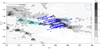 |
Fig. 7. Same as Fig. 6, but for clusters 6, 7, 8, and 9. |
| In the text | |
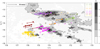 |
Fig. 8. Same as Fig. 6, but for clusters 10, 11, 12, 13, 14, 15, 16, 17, and 18. |
| In the text | |
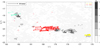 |
Fig. 9. Same as Fig. 6, but for clusters 19, 20, and 21. |
| In the text | |
|
Fig. 10. Comparison of the HMAC clustering results obtained in this study with the four populations of Taurus stars (blue, red, green, and cyan) identified by Luhman (2018) from the sample of known Taurus members (Table 1 of that paper). The bar chart indicates the number of stars of each population that are in common with the HMAC clusters. |
| In the text | |
|
Fig. 11. Kernel density estimate (for a kernel bandwidth of 1 km s−1) of the distribution of radial velocity measurements collected from the literature for 102 stars in the sample of cluster members obtained in our clustering analysis with HMAC. The tick marks in the horizontal axis indicate the individual measurements of each star. |
| In the text | |
|
Fig. 12. Posterior probability density function of the distance to the various molecular clouds of the Taurus complex. The solid and dashed lines indicate, respectively, the distances obtained from the Bayesian approach (see Sect. 5) and by inverting the mean parallax. |
| In the text | |
|
Fig. 13. Peculiar velocity of the stars in the various clouds of the Taurus complex projected onto the XY, YZ, and ZX planes. |
| In the text | |
|
Fig. 14. Mean spatial velocity of the stars projected towards the various molecular clouds of the Taurus complex. |
| In the text | |
|
Fig. 15. Comparison of the radial velocity of the stars (with respect to the LSR) with the centroid velocity of the 13CO emission extracted from the FCRAO maps at the position of each star. The black dashed line indicates a perfect correlation between the two measurements, and the colors respresent the various molecular clouds to which the stars belong. |
| In the text | |
Current usage metrics show cumulative count of Article Views (full-text article views including HTML views, PDF and ePub downloads, according to the available data) and Abstracts Views on Vision4Press platform.
Data correspond to usage on the plateform after 2015. The current usage metrics is available 48-96 hours after online publication and is updated daily on week days.
Initial download of the metrics may take a while.