The scale-free theory of stellar convection

C. Chiosi; S. Pasetto; E. Chiosi; D. Crnojević

doi:10.1051/0004-6361/202245321

Home

All issues

Volume 677 (September 2023)

A&A, 677 (2023) A85

Full HTML

Open Access

Issue		A&A Volume 677, September 2023


Article Number		A85
Number of page(s)		34
Section		Stellar structure and evolution
DOI		https://doi.org/10.1051/0004-6361/202245321
Published online		08 September 2023

A&A 677, A85 (2023)

A critical review and new results

C. Chiosi¹, S. Pasetto², E. Chiosi³ and D. Crnojević⁴

¹ Department of Physics & Astronomy, “Galileo Galilei”, University of Padua, Vicolo dell’Osservatorio 3, 35122 Padova, Italy
e-mail: cesare.chiosi@unipd.it
² H. Lee Moffitt Cancer Center & Research Institute, 12902 USF Magnolia Dr. SRR-4, Tampa, FL 33612, USA
³ INAF-Astronomical Observatory of Padua, Vicolo dell’Osservatorio 5, Padua, Italy
⁴ Department of Physics, University of Tampa, 401 West Kennedy Boulevard, Tampa, FL 33606, USA

Received: 28 October 2022
Accepted: 11 May 2023

Abstract

Context. A new, self-consistent, scale-free theory of stellar convection was recently developed (SFCT) in which velocities, dimensions, and energy fluxes carried by the convective elements are defined in a rest frame co-moving with the convective element itself. As the dynamics of the problem is formulated in a different framework with respect to the mixing length theory (MLT), the SFCT equations are sufficient to determine all the properties of stellar convection in accordance with the physics of the environment alone, with no need for the mixing length parameter (MLP). Subsequently, the SFCT was improved by introducing suitable boundary conditions at the surface of the external convective zones of the stars, and the first stellar models and evolutionary tracks on the Hertzsprung–Russell diagram were calculated.

Aims. The SFCT received alternatively positive and negative attention that spurred us to reconsider the whole problem. In this work, we aim to re-examine the physical foundations and results of the SFCT, elucidate some misconceptions on its physical foundations, reply to reported criticisms, and present some recent improvements to the SFCT.

Methods. The analysis was done using the same formalism of the previous studies, but novel arguments and demonstrations are added to better justify the controversial points, in particular the relaxation of instantaneous hydrostatic equilibrium between a convective element and the surrounding medium.

Results. The main results include (i) a novel detailed discussion of the boundary conditions to ensure that the temperature gradients in the outermost regions of a star are adequate for analyses of stability or instability in asteroseismology; (ii) a quantitative comparison with the MLT; and, finally, (iii) the recovery of the MLT as a particular case of the SFCT, but also in this case with no need for the MLP.

Conclusions. In conclusion, the SFCT is a step forward with respect to the classical MLT.

Key words: convection / stars: interiors / stars: evolution / stars: atmospheres / Sun: interior

© The Authors 2023

Open Access article, published by EDP Sciences, under the terms of the Creative Commons Attribution License (https://creativecommons.org/licenses/by/4.0), which permits unrestricted use, distribution, and reproduction in any medium, provided the original work is properly cited.

This article is published in open access under the Subscribe to Open model. Subscribe to A&A to support open access publication.

1. Introduction

Convection is one of the most studied energy-transport phenomena, and all the attempts to model it have their origin in studies of turbulence, starting from the pioneering work of Kolmogorov (e.g., Kolmogorov 1941) up to the most recent computational simulations in physics (e.g., Ishihara et al. 2009; Lohse & Xia 2010; Bec et al. 2010; Benzi et al. 2010; Rieutord & Rincon 2010; Meneveau 2011; Schmidt & Federrath 2011; da Silva et al. 2014; Schumacher et al. 2014) and astrophysics (e.g., Rempel & Cheung 2014; Hotta et al. 2015; Couch et al. 2015; Arnett et al. 2015; Gastine et al. 2015; Jiang et al. 2015; Kitiashvili et al. 2016; Lecoanet et al. 2016; Cristini et al. 2017). Excellent reviews can be found in Frisch (1998), Glatzmaier (2013), and Kupka & Muthsam (2017).

Stellar convection is customarily described by mixing-length theory (MLT), a simplified analytical formulation of the energy transport by convection, developed long ago by Böhm-Vitense (1958). The MLT stands on previous studies by Prandtl (1925), Biermann (1932, 1951), and Vitense (1953). In the literature, there are many versions of the MLT (see e.g., Cox & Giuli 1968; Kippenhahn & Weigert 1994; Weiss et al. 2004, and Kippenhahn et al. 2012), but all of them agree on the main points (see also Joyce & Tayar 2023 for a recent review of the subject).

The MLT stands on the basic assumption that the convective elements, during their existence and motion, are in strict hydrostatic equilibrium with the surrounding medium. This assumption is used to derive an elementary equation of motion for convective elements under the buoyancy and gravity forces to evaluate the kinetic energy and velocity of these elements, to evaluate the total amount of energy stored by a convective element when coming into existence, the energy lost by radiative losses to the medium during the element lifetime, and, finally, the net amount of energy released to the medium when the element dissolves in it (see Kippenhahn et al. 2012, Chap. 6, Sect. 6.1).

The MLT requires the computation of a scale length l_m to derive the dissipation rate of kinetic energy and to estimate a turbulent viscosity that is used in the computation of the convective flux and velocity (Pope 2000). The task is easy in the case of the pipe flow considered by Prandtl (1925) in which the length Λ is the pipe diameter itself (Pope 2000), much more difficult and uncertain in the case of stellar convection (see Canuto 2007a,b). To cope with the intrinsic uncertainty affecting the mixing length, this is assumed to be proportional to the local pressure scale height, l_m = Λ_m h_p, and the proportionality factor Λ_m (the mixing-length parameter, MLP) is tuned by comparing the stellar models to a calibrator, usually the Sun. No argument exists that the mixing-length parameter is the same in all stars and all evolutionary phases. Indeed, Λ_m is not constant in any sense: neither for a star of a given mass throughout its evolution nor for stars with different masses at the same age. This has been demonstrated by 3D-RHD simulations (see, e.g., Magic et al. 2015; Trampedach et al. 2013) or models of stellar convection related to these (Salaris & Cassisi 2015; Mosumgaard et al. 2020; Spada et al. 2021). Nevertheless, with the exception of new grids of stellar models made for use in asteroseismology, the vast majority of stellar models in the literature with multidisciplinary applications (analysis of star clusters, population synthesis, etc.) are affected by this significant drawback, that is, the calibration of the MLP and its consistency throughout the stellar masses and evolutionary phases.

To overcome these limits, several approaches have been proposed over the years. The simplest one (i) is the already mentioned fit of results obtained with an ML parameter to observations of different stars in the Hertzsprung–Russell diagram (HRD). The ML parameter in turn is assumed to be constant in stars of different masses and/or evolutionary stages (the standard view). Other alternative formulations allow the ML parameter to change with the position in the HRD (e.g., Pinheiro & Fernandes 2013). This approach is an extension of the original idea by Böhm-Vitense (1958) of the fit to the Sun. Helioseismology and/or asteroseismology (Brown & Gilliland 1994; Christensen-Dalsgaard 2002; Chaplin 2013; Chaplin & Miglio 2013) and much better data on the Sun produced by the Solar Heliospheric Observatory (SOHO) offer independent ways of testing stellar convection and constraining the ML theory in turn (e.g., Ulrich & Rhodes 1977; Kueker et al. 1993; Grossman 1996).

Time- dependent theories (ii) have been proposed by Kuhfuß (1986, 1987), Wuchterl & Feuchtinger (1998), and Flaskamp (2003), but they contain free parameters that must be calibrated.

Non-local theories (iii) are by Deng et al. (2006), Deng & Xiong (2008), and Canuto (2011e); however, they are difficult to use in stellar models because of their complexity and limited accuracy (Xiong 1986; Weiss & Flaskamp 2007). In general, non-local theories need several parameters to be fixed.

In a series of studies Canuto (2011a),b,c,d),e) elaborated a very general framework for the treatment of stellar convection and associated mixing processes (iv). The complex equations on which Canuto’s theory is grounded cannot be easily included in stellar models. To our knowledge, no attempt has been made so far by stellar evolutionists.

Next we have MLP-free (or scale-free) theories (v) by construction. It is worth mentioning a few examples such as Lydon et al. (1992), Balmforth (1992), or Canuto & Mazzitelli (1991), where other free parameters have been used instead of the mixing length. The turbulent scale length in Canuto & Mazzitelli (1991) is the most popular case.

Finally, in recent times sophisticated fully 3D-hydrodynamic simulations (vi) have been used to model and test convection. This approach requires large, time-consuming computational facilities to integrate the 3D-Navier-Stokes equations. In addition to the studies already mentioned above, we recall those of Ludwig et al. (1994, 1999), Bazán & Arnett (1998), Meakin & Arnett (2007), Collet et al. (2011), Chiavassa et al. (2011), Magic et al. (2013b, 2015), and Salaris & Cassisi (2015). The advantage here is that, unlike in the 1D integrations, parameter-free models of convection can be used. However, it has a very poor interpretative power: to extract a theoretical model from a simulation is not any simpler than writing a new one from scratch. To our knowledge, no full 1D theory based on these numerical approaches and suited to be included in stellar models has been derived.

Pasetto et al. (2014) developed the first self-consistent and scale-free theory of stellar convection, hereafter referred to as SFCT. Starting from the same physical context in which the classical MLT is developed, Pasetto et al. (2014) looked for a theory as simple as the MLT, but where no free parameter such as the MLP is present. The SFCT is formulated starting from a conventional solution of the Navier-Stokes/Euler equations, i.e., the Bernoulli equation for a perfect fluid, but expressed in a non-inertial reference frame comoving with the convective elements. In their formalism, the motion of stellar convective cells inside convectively unstable layers is entirely determined by a new system of equations that provide the subsonic solution for the convective energy transport that does not depend on any free parameter. The new theory is local in the usual sense of stellar convection as the equations are solved for a given mass shell, and the varying conditions at adjacent layers do not enter those equations: the various gradients refer to each mass shell. The equations contain the variable time, so in principle the solutions are time-dependent. In reality, what enters an SFCT-based stellar model is the result of an asymptotic limit configuration. All processes modeled by the dynamical equations occur on much shorter timescales. Therefore, in this respect, the SFCT is local and time independent, as is the classical MLT. In the SFCT, the convective elements can move radially and expand or contract simultaneously. In addition to the buoyancy force, the inertia of the fluid displaced by the convective elements and the effect of the convective element expansion or contraction on the buoyancy force is taken into account. Furthermore, the dynamical aspect of the problem is formulated in a reference frame comoving with the convective cells, and hence not requiring us to specify the path travelled by a cell. The resulting equations are sufficient to determine the radiative and convective fluxes together with the medium and element temperature gradients and the mean velocity and dimensions of the convective elements as a function of the environment physics (temperature density, chemical composition, opacity, etc.). Pasetto et al. (2014) applied the new theory to the case of the external layers of a stellar model representing the Sun calculated with the calibrated MLT by Bertelli et al. (2008). They described the outer convective zones of solar type stars and stars of different masses on the main-sequence band nicely. The predictions of the new theory are compared with those from the standard mixing-length paradigm for the most accurate calibrator, the Sun, with satisfactory results.

Subsequently, Pasetto et al. (2016) presented the first stellar models and companion evolutionary tracks on the HRD. The authors highlighted the role played by the boundary conditions at the surface of the external convective zone (in the regions where ionization of dominant elements including H, He, C, N, and O occurs) in determining the correct temperature gradient of the medium and the effective temperature of the star on the HRD. Keeping in mind that the SFCT to be applied needs to follow the temporal evolution of the size and displacement of the convective elements and therefore requires the time integration of the basic equations providing the velocity, the temperature gradients of the elements and medium, and the convective flux, Pasetto et al. (2016) derived suitable boundary conditions at the surface thus completing the set of fundamental equations. They also showed that the new SFCT yields stellar models as good as those based on the classical MLT with no need for the MLP.

Among the publications that have cited the SFCT in the meantime (e.g., Jin et al. 2015; Salaris & Cassisi 2015; Arnett et al. 2015; Rampazzo et al. 2016; Stancliffe 2016; Cassisi et al. 2016; Stancliffe et al. 2016; Muthsam & Kupka 2016; Moravveji et al. 2016; Kupka & Muthsam 2017; Cassisi 2017), the paper by Miller Bertolami et al. (2016) differs from other studies by clearly opposing the new model. The major controversial issues raised by these authors are (i) the assumption that convective elements and surrounding medium locally depart from mutual mechanical equilibrium; (ii) the intuitive argument that the radial upward or downward motion of convective elements occurs at a velocity significantly smaller than the expansion or contraction rate, and the use of the ratio of the vertical to expansion velocity as a convenient parameter to linearize the SFCT equations; (iii) the range of applicability of the SFCT that was claimed not to be of interest in astrophysical applications, actually in any physical regime; and other issues of minor relevance here. Surprisingly enough, after all these criticisms, they reached the same conclusions as us about the acceleration of the convective elements. Although the first issue raised by the criticism of Miller Bertolami et al. (2016) was already confuted in the paper by Pasetto et al. (2016, see their Section 3.3), the various issues were formally addressed by Pasetto et al. (2019) who clarified that the common assumption of the MLT that pressure balance is instantaneously achieved by the convective elements engenders misunderstanding of the mixing length itself and leads to results that contradict basic fluid dynamics. Finally, they showed how and why the study by Miller Bertolami et al. (2016) is essentially standing on misconceptions of the fundamentals of the basic fluid dynamics and leading to results that violate the Bernoulli equation.

Owing to the importance of the whole subject and the implications for the theory of stellar structure and evolution, in this paper we critically summarize the studies of Pasetto et al. (2014, 2016) and Pasetto et al. (2019), show that the hypothesis of strict pressure equilibrium between a convective element and its surroundings contradicts some basic principles of fluid dynamics, try to argue against the criticism of Miller Bertolami et al. (2016), and present some new results. More precisely, we carefully analyzed the physical meaning of the boundary conditions, focusing on the critical layer located just below the surface of a star in which the adiabatic temperature gradient suddenly drops as a result of the effects of incipient ionization. What happens in this critical region essentially determines the effective temperature. We propose a new set of boundary conditions that, applied to evolutionary models of low and intermediate mass stars, yield satisfactory results. The new boundary conditions confirm that the temperature stratification in the outermost convective zone of stars is better suited to asteroseismology studies. In this context, we introduce the analog of the MLP to read the results of the SFCT with the same language of the classical MLT so that vis-à-vis comparison is possible. Finally, we demonstrate that the MLT is a particular case of the SFCT when the strict pressure equilibrium between convective elements and their environment is introduced by hand. In such a case, the SFCT strictly yields the same results of the MLT, but without using any MLP to be calibrated.

In Sect. 2, we briefly present the main assumptions and fundamental equations of the SFCT; the algebraic numerical procedure to solve the equations of convection, in particular the quintic equation for the velocity of the convective element (the analog of the cubic equation of the MLT); the criteria to select the physically reasonable solutions for the velocity; and, finally, the boundary conditions at the very external layers of a convective region. In Sect. 3, we thoroughly discuss the issue of the pressure balance between the generic convective element and its surrounding medium, showing that this is not possible by first principles. While, on the average, a layer containing convective elements is in mechanical equilibrium with the rest of the star, the correct formulation of the physics of convection requires the pressure difference at the surface of a convective element and the medium in which it is embedded to be taken into account. In Sect. 4, we elucidate the relevance of correct temporal treatment of the pressure readjustment of the average convective element and its relation to the (always true) hydrostatic equilibrium of the whole star and provide a convincing demonstration of it. In Sect. 5, we discuss the boundary conditions at the surface of the external convective zone and present a few stellar models and evolutionary sequences calculated with the SFCT. The analysis is carried out in two steps; the first one adopts simple boundary conditions and presents the first stellar models; the second one refines the boundary conditions and presents the companion evolutionary sequence. In the second step, the temperature and velocity profiles in the region of ionization are much improved with respect to those of the first method in view of possible applications of the SFCT to problems of asteroseismology. In Sect. 6, with a simple numerical case, we check the SFCT and the limits of the so-called uniqueness theorem of Pasetto et al. (2014). In Sect. 7, we try to estimate the approximation introduced on the SFCT by neglecting the presence of turbulence. In Sect. 8, we briefly comment on the study by Miller Bertolami et al. (2016), highlighting some points of contradiction and inconsistency. In Sect. 9, we show that the MLT is part of the SFCT and present an approximate but very efficient algorithm for the calculation of the temperature gradients and convective flux in stellar models for the MLT-like version of the SFCT that does not require the mixing length parameter to be specified. The stellar models are indistinguishable from the standard ones with the canonical MLT. The algorithm can be easily implemented in any stellar evolution code. Finally, in Sect. 10 we comment on the new results, highlight the relevance of the correct physical treatment of the dynamics in the convective layers of a star, and draw some general conclusions.

2. The SFC theory in a nutshell

To ensure a better level of understanding, we briefly outline the SFCT by Pasetto et al. (2014, 2016) highlighting the main hypotheses, fundamental equations, and key results. No demonstration is given; they can be found in the original papers. The key idea of the new theory of stellar convection by Pasetto et al. (2014) is straightforward. Let us consider a rising convective element. In a 1D model of a star, because of the spherical symmetry, the motion occurs in the radial direction, while at the same time, the element increases its dimension. The opposite happens for an element sinking into the medium: radial motion and shrinkage. The upward (downward) motion and expansion (shrinkage) of the element are intimately related (indeed, the element rises because it expands and sinks because it shrinks). We remind the reader that only the radial motion is explicitly considered in the classical MLT, whereas expansion and shrinkage, although implicitly present, are not taken into account. Therefore, the trail to develop an alternative theory of convection is to look at the expansion (contraction), the radial motion being physically connected.

2.1. Formulation of the problem: General consideration

As already said, the theory we intend to develop is framed in the same physical context of the classical MLT; however, it contains a few differences: (i) the inclusion of both radial motion and expansion of convective elements, (ii) the relaxation of the instantaneous pressure equilibrium between a convective element and the surrounding medium, (iii) the presence of boundary conditions in the convective layers close to the surface. Common hypotheses are perfect fluid, no viscosity, no other forces but gravity and those due to pressure gradients, and zero vorticity and no turbulence. Finally, the SFCT derives the element velocity from the theory of potential flow (velocity potential).

Before presenting the founding hypotheses of the SFCT in more detail, it may be useful to summarize the many state-of-the-art numerical hydrodynamical simulations of convection that have been developed recently (see references in Sect. 1 and below), which help us to understand the physical nature and behavior of real convection in stars. To explain the extent to which they correspond to the convection envisaged by the MLT and shared by the SFCT, we provide the following summary.

Firstly, we have the assumption of zero vorticity and no turbulence. The necessity of accounting for turbulence when modeling stellar convection has been demonstrated, among others, in the following contexts. (i) Solar differential rotation for a star of solar type with a solar rotation rate can only be recovered in 3D global numerical simulations of solar convection at very high numerical resolution; hence, the simulation effectively has to be close enough to the “turbulent regime” (see e.g., Warnecke et al. 2021; Käpylä 2023). (ii) The turbulent pressure, P_t, contributes up to 12%–15% of total pressure in the superadiabatic layer (see e.g., Rosenthal et al. 1999) and also many other 3D-RHD simulations of solar granulation. This changes the frequencies of solar p modes compared to MLT models without turbulent pressure. Indeed, there are even several effects caused by the turbulence pressure P_t in this context (Houdek & Dupret 2015). Thus, P_t also has a key role in mode driving and damping for earlier type stars (see again Houdek & Dupret 2015) such as suppressing kappa-mechanism oscillations in stars of solar type while driving oscillations in late A- and early F-type main sequence stars. (iii) Stein & Nordlund (2000) and Kupka & Muthsam (2017) demonstrated the turbulent nature of solar surface convection. (iv) With regard to stellar mixing and overshooting, the role of turbulence is currently unknown in the context of stellar convective overshooting, since existing 3D hydrodynamical simulations have limited resolution (e.g., Käpylä 2019, 2021, and references therein).

Secondly, we have rising and sinking bubbles. State-of-the-art direct numerical simulations of convection in the Boussinesq approximation demonstrate that the “traditional picture” of convection being caused by rising and sinking bubbles cannot hold (see, e.g., Vincent & Yuen 1999, 2000; Johnston & Doering 2009; Goluskin & van der Poel 2016; Zhu et al. 2018; Stevens et al. 2018; Pandey et al. 2018, and others). These simulations show that plume-like features form, rise, or sink, and are “peeled off” due to local shear, that is, the Kelvin-Helmholtz instability. In 2D, vortices form. They usually grow through mergers more efficiently than by expansion. This holds for any range of Rayleigh numbers and Prandtl numbers currently accessible to direct numerical simulations including those typical for stellar surface convection. Thus, on the level of the Boussinesq approximation the physical picture of expanding bubbles (or other features) causing the convective flow does not hold, at least not on the scales with dominant contributions to (turbulent) kinetic energy, i.e., the scale of plume sizes and diameters. When density stratification is added to this picture, only a few things change (see, e.g., Porter & Woodward 2000; Cantin et al. 2000; Rogers et al. 2003; Zingale et al. 2015; Horst et al. 2020, and Kupka & Muthsam 2017).

Given these premises, there is no room left for theories such as the MLT and the SFCT, which obviously cannot compete with the results and details reached by numerical simulations. So, the major assumptions of zero-vorticity, radial motion combined with expansion of the convective elements, and potential flow are not adequate to represent the complexity of real convection. We are fully aware of these limitations of the MLT and SFCT in turn. However, since the MLT is still largely used in stellar model calculations (with a few exceptions), we are convinced that a refinement of the MLT is still worth undertaking. We do not intend to model effects that are out of reach for the present theory (e.g., turbulence and associated P_t, plume-like features, etc.), but we only aim to establish a model that, at least in the sense of a statistical average, predicts stratification of key physical quantities close enough to those present in real stars and satisfies the constraints imposed by observations. Furthermore, concerning the movements of convective elements, adding the expansion component to the vertical motion we hope to go closer to the real situations in which convective elements are found to continuously change their motion (velocity and direction), shape, and size. However, for detailed flow predictions the rising and sinking bubble picture is certainly incorrect. There remains the assumption of the flow potential and velocity potential that is strictly only possible in the absence of vorticity. Since no vorticity is one of the assumptions, the use of the flow potential is at least consistent with it.

2.2. Formulation of the problem: Main hypotheses

Main assumptions of the SFCT are those outlined hereafter. (i) The stellar medium is a perfect fluid governed by a suitable equation of state (EoS) that can change with time t and position cx (and in which the presence of viscosity can be neglected). A perfect fluid is intrinsically unstable and turbulent; therefore, the higher the Reynolds number, the better the above approximation of neglecting the viscous terms holds. On macroscopic scales, the stellar interiors are in mechanical and thermodynamical equilibrium; all other forces (due to viscosity, rotation, and magnetic fields) are neglected, except those due to gravity and pressure gradients.

(ii) The fluid is of course compressible, a requisite that is essential for the stacking of structures (Porter & Woodward 2000); however, in order to make use of the flow potential (or velocity potential) we suppose that on a suitable local distance scale the fluid can be considered as incompressible. The concept of a local distance scale is defined here from a heuristic point of view. This length should be long enough to contain a significant number of convective elements so that a statistical formulation is possible when describing the mean convective flux of energy, but small enough so that the distance traveled by the convective element is short compared to the typical distance over which significant gradients in temperature, density, pressure, and so on can develop (i.e., those gradients are locally small).

(iii) Using the concept of velocity potential also requires the fluid to be describable neglecting turbulence. This is rather difficult to achieve, and, at first sight, it goes against common sense because of the turbulent nature of the convective phenomenon. However, the example of the roaring water flowing downhill in a mountain torrent comes to our aid. Water always flows downhill despite the many vortices of different sizes; therefore, as long as we are interested in water’s bulk velocity, the presence of turbulence can be ignored. The same applies to stellar convection, provided we limit ourselves to obtaining a first-order velocity estimate.

To support this view, we evaluated the flux of total kinetic energy associated to the motion of convective elements and compared it to the radiative luminosity. The analysis is limited to the Sun. The numerical simulations show that the turbulent pressure contributes to the total pressure by about 15%, i.e., P_t/P ≃ 0.15; the ratio P_t/P is in turn expressed as $P_{t} / P = (1 / 3) Γ_{1} {(\bar{u} / u_{s})}^{2}$ $P_{\mathrm{t}}/P = (1/3) \Gamma_1 (\bar{u} /u_{\mathrm{s}})^2$ , where Γ₁ is the first adiabatic exponent (or gamma), $\bar{u}$ $\bar{u}$ the mean velocity of convective elements, and u_s the sound velocity (for the formalism, see Cox & Giuli 1968). Using Γ₁ = 5/3 for a perfect gas, we obtain $P_{t} / P = (5 / 9) {(\bar{u} / u_{s})}^{2}$ $P_{\mathrm{t}}/P = (5/9) (\bar{u} /u_{\mathrm{s}})^2$ , which, when inverted, yields ${\bar{u}}^{2} = (9 / 5) u_{s}^{2} (P_{t} / P)$ $\bar{u}^2 = (9/5)u_{\mathrm{s}}^2 (P_{\mathrm{t}} / P)$ . Let us now pose β = (P_t/P); therefore, ${\bar{u}}^{2} = (9 / 5) u_{s}^{2} β$ $\bar{u}^2 = (9/5)u_{\mathrm{s}}^2 \beta$ .

The flux per unit area of kinetic energy and total kinetic luminosity L_k are

$\begin{matrix} F_{k} = \frac{1}{2} ρ_{c} {\bar{u}}^{3} L_{k} = 4 π R_{e}^{2} F_{k}, \end{matrix}$ $\begin{aligned} F_{\rm k} = \frac{1}{2} \rho _{\rm c} \bar{u}^3\, \quad L_{\rm k} = 4\pi R_{\rm e}^2 F_{\rm k}, \end{aligned}$

where ρ_c is the mean density of the convective region. The demonstration of F_k is straightforward.

Assuming typical values for each variable entering the above expressions, we were able to proceed to numerical evaluations. In the case of Sun, we may adopt R_e = 7 × 10¹⁰ cm, $\bar{u} ≃ 1.5$ $\bar{u} \simeq 1.5$ km s⁻¹, u_s ≃ 17 km s⁻¹, ρ_c ≃ 10⁻⁶ gr cm⁻³, and lifetime of convective elements t_c in the range of 1–100 min (Cox & Giuli 1968).

Let us now derive F_k in two limit cases. In the first case, there is no turbulence; hence, $\bar{u} ≃ 1.5$ $\bar{u} \simeq 1.5$ km s⁻¹, F_k = 1.688 × 10⁹ erg s⁻¹ cm⁻², which, multiplied by the area of the stellar surface (6.15 × 10²² cm²), yields the kinetic luminosity L_k ≃ 1.038 10³² erg s⁻¹ to be compared to the luminosity of the Sun L_⊙ ≃ 4 × 10³³ erg s⁻¹, i.e., L_k/L_⊙ ≃ 0.026. The kinetic luminosity associated with the motion of convective elements is negligible compared to the optical luminosity.

In the second case, there is turbulence, and hence ${\bar{u}}^{2} = (9 / 5) u_{s}^{2} β$ $\bar{u}^2 = (9/5)u_{\mathrm{s}}^2 \beta$ . Assuming β = 0.15 and u_s ≃ 17 km s⁻¹, we obtain F_k = 17.797 × 19⁹ erg s⁻¹ cm⁻², which, multiplied by the area of the stellar surface (6.15 × 10²² cm²), yields the kinetic luminosity L_k ≃ 1.095 × 10³³ erg s⁻¹, i.e., L_k/L_⊙ ≃ 0.27. The ratio is about ten times higher than in the previous case. The effect of turbulence cannot be neglected. Part of the energy carried by the luminosity (built deep inside a star) goes into turbulent kinetic energy to be dissipated. However, the estimate for L_k can be lowered considering that we have taken an upper limit for P_t/P and ρ_c (it can be lower by a certain factor in the regions of interest, i.e., the most external ones where the MLT and SFCT are at work). Therefore, most likely L_k < L_⊙. If so, it would allow us to say that turbulence can be neglected as a first approximation. This may not hold in the case of the very bright, extended RGB stars where P_t/P can be close or even higher than our limit; however, at the same time the mean density is much lower, so a simple evaluation is not possible. This is a point to keep in mind.

In conclusion, the approximation of neglecting turbulence in the SFCT has some justification. Certainly, this approximation is not worse than the estimate made in the MLT by converting an arbitrary fraction of the work done by the buoyancy force into kinetic energy of the fluid and estimating from it the typical value of the velocity. In any case, in Sect. 7 we go over this again, presenting an estimate of the uncertainty on the velocity induced by neglecting turbulence.

The same assumptions are usually made in the case of the classical MLT. In this context, the concept of potential flow can be used, that is, a generic velocity field can be derived from the gradient of a suitable potential (see Landau & Lifshitz 1959, Chap. 1).

2.3. Pressure equilibrium between elements and medium

The motion of a generic convective element can be described by the integral of the Navier-Stokes equations, that is, the Bernoulli equation, in which we neglect magnetic fields and viscous terms (typical of high-Reynold-number fluids in which viscous terms are small compared to inertial terms). We also neglect the terms of kinetic energy dissipation, and the velocity field is derived from the velocity potential formalism.

In addition to this, the theory of convection of Pasetto et al. (2014, 2016) is based on the notion that a convective element cannot be in strict mechanical equilibrium with its surrounding medium and hence takes local deviations from rigorous hydrostatic equilibrium into account. In other words, the stellar plasma is not in mechanical equilibrium on the surface of the expanding or contracting convective element, while the latter is moving outward or inward. A convective element coming into existence for whatever reason and expanding into the medium represents a perturbation of the local pressure that cannot instantaneously recover the pressure balance with the surrounding. The condition of rigorous pressure equilibrium with the stellar medium is only met “far away” from the surface of a convective element. This means that from a macroscopic point of view each layer of a convective zone is in rigorous mechanical equilibrium (gravity is balanced by the forces generated by pressure gradients), but the equations governing the onset and motion of convective elements take this virtual deviation from pressure balance into account. This more general description of the physical conditions in which convective elements form and move leads to a better description of the motion of convective elements compared to the simple assumption of instantaneous pressure equilibrium based on the high value of the sound velocity, as is commonly written in many textbooks on stellar astrophysics (e.g., Cox & Giuli 1968; Kippenhahn et al. 2012). This issue has been examined in great detail by Pasetto et al. (2019), to which the reader should refer, showing that by first principles, no instantaneous pressure equilibrium is possible at the surface of a convective element and its surroundings. Owing to its relevance, we reconsider this key point in detail in Sect. 3.

For the reasons amply illustrated by Pasetto et al. (2014, 2016), the mathematical formulation of the whole problem becomes easy to handle if instead of using an inertial reference frame S₀ centered on a star’s center we use a non-inertial lagrangian frame of reference S₁ centered on and co-moving with the generic convective element. The two reference frames are schematically shown in Fig. 1. In S₁, the element is at rest with respect to the surrounding medium while it expands or contracts into it.

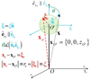Fig. 1.

Schematic representation of a convective element seen in the inertial frame S_O (origin at the point O) and in the co-moving frame S₁ (origin at the point O′). The element is represented as a spherical body for simplicity. The center of the sphere indicated as O′ also corresponds to the position of the element in S₀. The generic dimension of the convective element as seen in S₁ is indicated by ξ_e. Reproduced from Pasetto et al. (2016).

2.4. Bernoulli equation in frames S₀ and S₁

With the physical assumptions made above for the stellar fluid and the forces in action, Euler’s equation

$\begin{matrix} \frac{\partial ρ v_{0}}{\partial t} + 〈 \nabla_{x}, P + ρ v_{0} v_{0} 〉 - ρ \sum_{i}^{n_{i} F_{i}} = 0, \end{matrix}$ $\begin{aligned} \frac{{\partial \rho {{\boldsymbol{v}}_0}}}{{\partial t}} + \left\langle {{\nabla _{\boldsymbol{x}}},{\boldsymbol{P}} + \rho {{\boldsymbol{v}}_0}{{\boldsymbol{v}}_0}} \right\rangle - \rho \sum \limits _i^ {{n_i}{{\boldsymbol{F}}_i}} = 0, \end{aligned}$ (1)

the continuity equation

$\begin{matrix} \frac{\partial ρ}{\partial t} + 〈 \nabla_{x}, ρ v_{0} 〉 = 0, \end{matrix}$ $\begin{aligned} \frac{{\partial \rho }}{{\partial t}} + \left\langle {\nabla _{\boldsymbol{x}} ,\rho {{\boldsymbol{v}}_0}} \right\rangle = 0, \end{aligned}$ (2)

and the identity

$\begin{matrix} 〈 \nabla_{x}, ρ v_{0} v_{0} 〉 = v_{0} ρ ⟨ \nabla_{x}, v_{0} ⟩ + ρ ⟨ v_{0}, \nabla_{x} v_{0} ⟩ \end{matrix}$ $\begin{aligned} \left\langle {\nabla _{\boldsymbol{x}} ,\rho {{\boldsymbol{v}}_0}{{\boldsymbol{v}}_0}} \right\rangle = {{\boldsymbol{v}}_0}\rho \langle {\nabla _{\boldsymbol{x}}, {{\boldsymbol{v}}_0}} \rangle + \rho \langle { {{\boldsymbol{v}}_0}, \nabla _{\boldsymbol{x}} {{\boldsymbol{v}}_0}} \rangle \end{aligned}$ (3)

yield

$\begin{matrix} ρ \frac{\partial v_{0}}{\partial t} + 〈 \nabla_{x}, P 〉 + 〈 ρ v_{0}, \nabla_{x} v_{0} 〉 - \sum_{i}^{n_{i} F_{i}} = 0 . \end{matrix}$ $\begin{aligned} \rho \frac{{\partial {{\boldsymbol{v}}_0}}}{{\partial t}} + \left\langle {{\nabla _{\boldsymbol{x}}},{\boldsymbol{P}}} \right\rangle + \left\langle {\rho {{\boldsymbol{v}}_0},{\nabla _{\boldsymbol{x}}}{{\boldsymbol{v}}_0}} \right\rangle - \sum \limits _i^ {{n_i}{{\boldsymbol{F}}_i}} = 0. \end{aligned}$ (4)

In Eq. (4), P is the pressure tensor, F the force acting on every particle of the fluid, n_i the number density of every type of fluid particle, and the term ⟨*,*⟩ denote the inner product. With the above assumption, no electric field E is present. This is a partial differential equation (PDE) where the quantities involved are functions of time t and position x in the given inertial reference frame S₀(O,x) centered in O. Hereafter, we omit writing this dependence explicitly to simplify the notation (unless specified otherwise for the sake of better understanding).

Stellar interiors are well represented by a perfect fluid in local thermodynamical equilibrium (LTE), that is, each elemental component, n_i of the fluid is isotropic, homogeneous, in mechanical equilibrium, and obeys the conditions of detailed balance with any other component n_j. Therefore, we can simplify ⟨∇_x,P⟩ = ∇_xP. Furthermore, as the force acting on the fluid particle is non-diffusive, i.e., in our case the gravity F_i = m_ig on the particles of the ith species, we can assume that $\sum_{i}^{n_{i} F_{i}} = \sum_{i}^{m_{i} n_{i} g} = (\sum_{i}^{m_{i} n_{i}}) g = ρ g$ $\sum\limits_i^ {{n_i}{\boldsymbol{F_i}}} = \sum\limits_i^ {{m_i}{n_i}{\boldsymbol{g}}} = \left( {\sum\limits_i^ {{m_i}{n_i}} } \right){\boldsymbol{g}} = \rho {\boldsymbol{g}}$ . With these simplifications, Eq. (4) becomes

$\begin{matrix} ρ \frac{\partial v_{0}}{\partial t} + \nabla_{x} P + 〈 ρ v_{0}, \nabla_{x} v_{0} 〉 - ρ g = 0 . \end{matrix}$ $\begin{aligned} \rho \frac{{\partial {{\boldsymbol{v}}_0}}}{{\partial t}} + {\nabla _{\boldsymbol{x}}}P + \left\langle {\rho {{\boldsymbol{v}}_0},{\nabla _{\boldsymbol{x}}}{{\boldsymbol{v}}_0}} \right\rangle - \rho {\boldsymbol{g}} = 0. \end{aligned}$ (5)

We now introduce the concept of a potential flow (e.g., Landau & Lifshitz 1959, Chap. 1):

$\begin{matrix} \nabla_{x} \times v_{0} = 0 \Leftrightarrow \exists Φ_{v_{0}} | v_{0} = \nabla_{x} Φ_{v_{0}}, \end{matrix}$ $\begin{aligned} {\nabla _{\boldsymbol{x}}} \times {{\boldsymbol{v}}_0} = 0 \Leftrightarrow \exists {\Phi _{{{\boldsymbol{v}}_0}}}\, | \, \, \,{{\boldsymbol{v}}_0} = {\nabla _{\boldsymbol{x}}}{\Phi _{{{\boldsymbol{v}}_0}}}, \end{aligned}$

with Φ_v₀ being the velocity potential. In particular, with the help of the vector relation

$\begin{matrix} 〈 v_{0}, \nabla_{x} v_{0} 〉 = \frac{1}{2} \nabla_{x} 〈 v_{0}, v_{0} 〉 - v_{0} \times (\nabla_{x} \times v_{0}) \end{matrix}$ $\begin{aligned} \left\langle {{{\boldsymbol{v}}_0},{\nabla _{\boldsymbol{x}}}{{\boldsymbol{v}}_0}} \right\rangle = \frac{1}{2}{\nabla _{\boldsymbol{x}}}\left\langle {{{\boldsymbol{v}}_0},{{\boldsymbol{v}}_0}} \right\rangle - {{\boldsymbol{v}}_0} \times \left( {{\nabla _{\boldsymbol{x}}} \times {{\boldsymbol{v}}_0}} \right) \end{aligned}$

and remembering that the curl of a gradient is null,

$\begin{matrix} \nabla_{x} \times v_{0} = \nabla_{x} \times \nabla_{x} Φ_{v_{0}} = 0, \end{matrix}$ $\begin{aligned} {\nabla _{\boldsymbol{x}}} \times {{\boldsymbol{v}}_0} = {\nabla _{\boldsymbol{x}}} \times {\nabla _{\boldsymbol{x}}}{\Phi _{{{\boldsymbol{v}}_0}}} = 0, \end{aligned}$

we are able to write Eq. (5) as

$\begin{matrix} \nabla_{x} (\frac{\partial Φ_{v_{0}}}{\partial t} + \frac{P}{ρ} + \frac{{∥ v_{0} ∥}^{2}}{2} + Φ_{g}) = 0, \end{matrix}$ $\begin{aligned} {\nabla _{\boldsymbol{x}}}\left( {\frac{{\partial {\Phi _{{{\boldsymbol{v}}_0}}}}}{{\partial t}} + \frac{P}{\rho } + \frac{{{{\left\Vert {{{\boldsymbol{v}}_0}} \right\Vert}^2}}}{2} + {\Phi _{\boldsymbol{g}}}} \right) = 0, \end{aligned}$

where the relation between gravitational force and gravitational potential g = −∇_xΦ_g has been adopted. The symbol ∥…∥ indicates the standard Euclidean norm of a generic vector. Finally, the integration of the previous equation leads to Bernoulli’s equation in an inertial reference system S₀ centered at the center of the star. With the formalism developed here,

$\begin{matrix} \frac{\partial Φ_{v_{0}}}{\partial t} + \frac{P}{ρ} + \frac{{∥ v_{0} ∥}^{2}}{2} + Φ_{g} = f (t) . \end{matrix}$ $\begin{aligned} \frac{{\partial {\Phi _{{{\boldsymbol{v}}_0}}}}}{{\partial t}} + \frac{P}{\rho } + \frac{{{{\left\Vert {{{\boldsymbol{v}}_0}} \right\Vert}^2}}}{2} + {\Phi _{\boldsymbol{g}}} = f\left( t \right). \end{aligned}$ (6)

This equation is one describing the stellar plasma in which convection is at work. In this particular form it stands on the use of the potential flow. It could be extended to include diffusion and turbulence. However, as the primary goal here is to derive the mechanics of convection from simple principles, the current approach is adequate for our aims. Diffusion and turbulence can eventually be included using the same formalism in a future study. In the context of thermal convection, it is worth recalling that the Boussinesq (Spiegel & Veronis 1960) and inelastic (Gough 1969) approximations would be more valuable alternatives worthy of being investigated. Nevertheless, for the aims of this study, the potential flow approximation turns out to be satisfactory, as confirmed by our numerical investigation described in Sect. 6.

After these preliminary remarks, we are now in the position to state the queries that we intend to address as follows: the main target of stellar convection is to find a solution of Eq. (6) linking the physical quantities characterizing the stellar interiors such as pressure, density, temperature, velocities, and so on, and the mechanics governing the motion of the convective elements as functions of the fundamental temperature gradients to pressure, i.e., the radiative gradient ∇_rad, the adiabatic gradient ∇_ad, the local gradient of the star $\nabla \equiv | \frac{d ln T}{d ln P} |$ $\nabla \equiv \left| {\frac{{\mathrm{d}\ln T}}{{\mathrm{d}\ln P}}} \right|$ , the convective element gradient ∇_e, and the molecular weight gradient $\nabla_{μ} \equiv | \frac{d ln μ}{d ln P} |$ ${\nabla _\mu } \equiv \left| {\frac{{\mathrm{d}\ln \mu }}{{\mathrm{d}\ln P}}} \right|$ .

The task is difficult because of the large number of variables involved to describe the convective element’s physics and the stellar interiors, both of which are poorly known. Mathematically, the problem translates into a system of algebraic-differential equations (ADEs). In the MLT, the solution of this ADE is simplified to an algebraic system of equations by introducing a statistical description of the motion, size, lifetime, and so on, of the convective elements. In this way, the complicated pattern of possible convective elements is reduced to a mean element whose dimensions and path are simply supposed to be l_m = Λ_mh_p, where Λ_m is a parameter to be fixed by comparing real stars (the Sun) to stellar models. Once Λ_m is calibrated in this way, it is assumed to be the same for all stars of any mass, chemical composition, and evolutionary stage. This is indeed a strong assumption. The majority of stellar models in the literature are calculated with this assumption. However, it is worth recalling that a few new grids of stellar models, in particular those made for the use in asteroseismology, are constructed by calibrating Λ_m with 3D-RHD simulations of stellar surface convection (Salaris & Cassisi 2015; Mosumgaard et al. 2020; Spada et al. 2021).

The solution of the Bernoulli equation establishes the dependence of the mechanics governing the motion of convective elements, acceleration, and velocities on the fundamental temperature gradients to pressure, i.e., the radiative gradient ∇_rad, the adiabatic gradient ∇_ad, the ambient gradient ∇, the convective element gradient ∇_e, and the gradient in molecular weight $\nabla_{μ} = {| \frac{\partial ln μ}{\partial ln P} |}_{t}$ $\nabla _{\mu }= \left| \frac{\partial \ln \mu} {\partial \ln P} \right|_{\mathrm{t}}$ , which in turn are all functions of the physical quantities characterizing the stellar medium such as pressure, density, temperature, and so on. The problem, however, can be tackled in a relatively straightforward fashion making use of the concept and formalism of the velocity potential.

2.5. Velocity potential in the accelerated frame S₁

Having set the physical background of our equations, we go back to the lagrangian reference frame S₁ : (O′,ξ) co-moving with and centered on the center of the generic eddy. From the geometry shown in Fig. 1, the radius of a generic convective element of spherical shape is indicated as |x_e − x_O′| = r_e in S₀ and |x_e − x_O′| = ξ_e in S₁. In this reference frame, the Bernoulli Eq. (6) reads

$\begin{matrix} \frac{\partial Φ_{{v^{'}}_{0}}^{'}}{\partial t} + \frac{P}{ρ} + \frac{{∥ {v^{'}}_{0} ∥}^{2}}{2} + Φ_{g} = f (t) - 〈 A, ξ 〉, \end{matrix}$ $\begin{aligned} \frac{{\partial {\Phi ^{\prime } _{{{\boldsymbol{v^\prime }}_0}}}}}{{\partial t}} + \frac{P}{\rho } + \frac{{{{\left\Vert {{{\boldsymbol{v^\prime }}_0}} \right\Vert}^2}}}{2} + {\Phi _{\boldsymbol{g}}} = f\left( t \right) -\left\langle {{\boldsymbol{A}},{\boldsymbol{\xi }}} \right\rangle ,\end{aligned}$ (7)

where the relative acceleration of the two reference frames is indicated with A. Pasetto et al. (2014) demonstrated that in S₁ the total potential flow outside the surface of a moving and expanding/contracting element is given by

$\begin{matrix} Φ^{'} = - 〈 v, ξ 〉 (1 + \frac{1}{2} \frac{ξ_{e}^{3}}{{∥ ξ ∥}^{3}}) - \frac{{\dot{ξ}}_{e} ξ_{e}^{2}}{∥ ξ ∥}, \end{matrix}$ $\begin{aligned} \Phi ^\prime = - \left\langle {{\boldsymbol{v}},{\boldsymbol{\xi }}} \right\rangle \left( {1 + \frac{1}{2} \frac{{\xi _{\rm e}^3}}{{{{\left\Vert {\boldsymbol{\xi }} \right\Vert}^3}}}} \right) - \frac{{{{\dot{\xi }}_{\rm e}}\xi _{\rm e}^2}}{{\left\Vert {\boldsymbol{\xi }} \right\Vert}}, \end{aligned}$ (8)

so that the corresponding velocity in S₁ can be written as

$\begin{matrix} {v^{'}}_{0} = {\frac{3}{2} (〈 v, \hat{n} 〉 \hat{n} - v) + {\dot{ξ}}_{e} \hat{n} |}_{∥ ξ ∥ = ξ_{e}}, \end{matrix}$ $\begin{aligned} {{{\boldsymbol{v^\prime }}}_0} = {\left. {\frac{3}{2}\left( {\left\langle {{\boldsymbol{v}}, {\boldsymbol{\hat{n}}}} \right\rangle {\boldsymbol{\hat{n}}} - {\boldsymbol{v}}} \right) + {{\dot{\xi }}_{\rm e}}{\boldsymbol{\hat{n}}}} \right|_{\left\Vert {\boldsymbol{\xi }} \right\Vert = {\xi _{\rm e}}}}, \end{aligned}$ (9)

where $\hat{n} \equiv ξ / ∥ ξ ∥$ ${\boldsymbol{\hat n}} \equiv {\boldsymbol{\xi }}/\left\| {\boldsymbol{\xi }} \right\|$ and the meaning of the symbols is read out from Fig. 1. The above expression is evaluated at the surface of the convective element. It is also easy to show that this equation yields correct results at the surface of the element once written in spherical coordinates where θ is the angle between the unitary vectors ${\hat{e}}_{z}$ ${\boldsymbol{\hat e}_z}$ and $\hat{n}$ $\boldsymbol{\hat{n}}$ . Therefore, Eq. (7) reads

$\begin{matrix} {\frac{\partial Φ^{'}}{\partial t} |}_{∥ ξ ∥ = ξ_{e}} = - \frac{3}{2} ξ_{e} 〈 A, \hat{n} 〉 - \frac{3}{2} {\dot{ξ}}_{e} 〈 v, \hat{n} 〉 - {\ddot{ξ}}_{e} ξ_{e} - 2 {\dot{ξ}}_{e}^{2} . \end{matrix}$ $\begin{aligned} {\left. {\frac{{\partial \Phi^\prime }}{{\partial t}}} \right|_{\left\Vert {\boldsymbol{\xi }} \right\Vert={\xi _{\rm e}}}} = - \frac{3}{2}{\xi _{\rm e}}\left\langle {{\boldsymbol{A}},{\boldsymbol{\hat{n}}}} \right\rangle - \frac{3}{2}{\dot{\xi }_{\rm e}} \left\langle {{\boldsymbol{v}},{\boldsymbol{\hat{n}}}} \right\rangle - {\ddot{\xi }_{\rm e}}{\xi _{\rm e}} - 2\dot{\xi }_{\rm e}^2. \end{aligned}$ (10)

Finally, by adjusting the PDE boundary conditions we can prove that $f (t) = \frac{‖ v ‖}{2}$ $f(t) = \frac{\|{\boldsymbol{v}\|}} {2}$ , and by inserting Eqs. (8), (9), and (10) into Eq. (7), we are led to the general relation

$\begin{matrix} \frac{v^{2}}{2} (\frac{9}{4} {sin}^{2} θ - 1) - v {\dot{ξ}}_{e} \frac{3}{2} cos θ + (\frac{P}{ρ} + Φ_{g}) = \\ + a ξ_{e} (\frac{3}{2} cos θ - cos ϕ) + {\ddot{ξ}}_{e} ξ_{e} + \frac{3}{2} {\dot{ξ}}_{e}^{2}, \end{matrix}$ $\begin{aligned}&\frac{{{{ v}^2}}}{2}\left( {\frac{9}{4}{{\sin }^2}\theta - 1} \right)- { v}{{\dot{\xi }}_{\rm e}} \frac{3}{2}\cos \theta + \left( {\frac{P}{\rho } + {\Phi _{\boldsymbol{g}}}} \right) = \nonumber \\&+ a{\xi _{\rm e}}\left( {\frac{3}{2}\cos \theta - \cos \phi } \right) + {{\ddot{\xi }}_{\rm e}}{\xi _{\rm e}} + \frac{3}{2}\dot{\xi }_{\rm e}^2, \end{aligned}$ (11)

where a = ∥A∥ is the norm of the acceleration, ϕ the angle between the direction of motion of the fluid as seen from S₁ and the acceleration direction, and θ the angle between the radius ξ in S₁ and the velocity v (hereafter v = ∥v∥).

2.6. The relationship between radial motion and expansion-contraction

In order to obtain equations that can be analytically dealt with, Pasetto et al. (2014) limited their analysis to the linear regime. To this aim, we need a parameter whose value remains small enough to ensure that the linearization of the fundamental equations is possible. Furthermore, we limit ourselves to the case of subsonic stellar convection.

In our picture, the motion of a generic convective element can be described by a radial upward or downward displacement with velocity v and, at each position, by expansion or contration at rate ${\dot{ξ}}_{e}$ $\boldsymbol{\dot \xi_{\mathrm{e}}}$ . In the limit t → ∞, the two motions satisfy the relation

$\begin{matrix} ∥ v ∥ ≪ ∥ {\dot{ξ}}_{e} ∥ . \end{matrix}$ $\begin{aligned} \left\Vert {\boldsymbol{v}} \right\Vert \ll \left\Vert {{{{\boldsymbol{\dot{\xi }}}}_{\rm e}}} \right\Vert . \end{aligned}$ (12)

This approach turns out to be a convenient assumption for a number of reasons. The upward or inward displacement of an element must oppose gravity and density increase, respectively, both concurring to slow down its motion. The expansion of a convective element also occurs throughout gradients of gravity and density. Over the short lifetime of a convective eddy, we can envisage the expansion as preferentially occurring toward regions of lower or nearly constant density and regions of nearly constant gravity. It is intuitive to imagine that this would occur faster than the vertical displacement of the whole convective element. Finally, the velocities of both motions are supposed to always remain smaller than the local sound velocity.

We are aware of the limitations imposed by this naive approximation to the real description of a convective element before dissolving into the surrounding medium. Indeed, it is not supported by observations because such expansion or contraction processes would leave their fingerprints on the kinetic energy spectra that, in contrast, are not detected and by the numerical simulations in which motions and shapes of fluid elements are far more chaotic and unpredictable. The only thing we can claim is that in comparison with the MLT with its instantaneous adjustment to the ever changing situations, in the SFCT the fluid motion is modeled by taking into account that such processes require a finite time to occur. Since over the length scales of interest this occurs on shorter timescales than the vertical enthalpy flux, the associated velocities have to be faster. In the MLT, with its spontaneous and instantaneous adjustment, they are infinite.

Thanks to this assumption, we may take the ratio $ε \equiv \frac{∥ v ∥}{∥ {\dot{ξ}}_{e} ∥} ≪ 1$ $\varepsilon \equiv \frac{{\left\| {\boldsymbol{\mathit{v}}} \right\|}}{{\left\| {{{{\boldsymbol{\dot \xi }}}_{\mathrm{e}}}} \right\|}} \ll 1$ in the limit t → ∞ as the parameter used to develop a linear theory. In such a case, Eq. (11) becomes

$\begin{matrix} {\ddot{ξ}}_{e} ξ_{e} + \frac{3}{2} {\dot{ξ}}_{e}^{2} + \frac{a ξ_{e}}{2} = 0, \end{matrix}$ $\begin{aligned} {{{\ddot{\xi }}_{\rm e}}{\xi _{\rm e}} + \frac{3}{2}\dot{\xi }_{\rm e}^2 + \frac{{a{\xi _{\rm e}}}}{2} = 0}, \end{aligned}$ (13)

which determines the temporal evolution of the expansion rate of a convective element and where, differently from Eq. (10), a is constant. The straight solution of this equation is difficult but feasible. We refer the reader to Pasetto et al. (2014) for all mathematical details.

Posing χ ≡ ξ_e/ξ_e0 and τ ≡ t/t₀ (ξ_e0 and t₀ two arbitrary small normalization factors), one obtains a second order differential equation in χ(τ) from Eq. (13), the solution of which yields the dimensionless size of a generic convective element as a function of a dimensionless time. The solution χ(τ) is

$\begin{matrix} χ (τ) = \frac{1}{4} τ^{2} + \frac{\sqrt{π} Γ (7 / 8)}{Γ (3 / 8)} τ + \frac{π Γ {(7 / 8)}^{2}}{Γ {(3 / 8)}^{2}}, \end{matrix}$ $\begin{aligned} \chi \left( \tau \right) = \frac{1}{{{4}}}{\tau ^2} + \frac{{\sqrt{\pi }\Gamma \left( 7/8 \right)}}{{\Gamma \left( 3/8 \right)}}\tau + \frac{{\pi \Gamma {{\left( 7/8 \right)}^2}}}{{\Gamma {{\left( 3/8 \right)}^2}}}, \end{aligned}$ (14)

whose asymptotic dependence is ∼τ² plus lower order correction terms. As a consequence, the time-averaged value $χ (τ) = \frac{1}{τ} \int_{0}^{τ} χ (τ^{'}) d τ^{'}$ $\chi \left( \tau \right) = \frac{1}{\tau }\int_0^\tau {\chi \left( {\tau^\prime} \right)\mathrm{d}\tau^\prime}$ will also grow with the same temporal proportionality:

$\begin{matrix} χ (t) = \frac{τ^{2}}{12} + \frac{\sqrt{π} τ Γ (7 / 8)}{2 Γ (3 / 8)} + \frac{π Γ {(7 / 8)}^{2}}{Γ {(3 / 8)}^{2}}, \end{matrix}$ $\begin{aligned} \chi \left( t \right) = \frac{{{\tau ^2}}}{{12}} + \frac{{\sqrt{\pi }\tau \Gamma \left( 7/8 \right)}}{{2\Gamma \left( 3/8 \right)}} + \frac{{\pi \Gamma {{\left( 7/8 \right)}^2}}}{{\Gamma {{\left( 3/8 \right)}^2}}} , \end{aligned}$ (15)

where we indicated with the same symbol χ both the solution χ(τ), (14), and its time-averaged value χ(t), (15)¹. It is worth noting that the starting Eq. (11) contains the relative acceleration and has been expressed in S₁, where the expanding contracting or convective element is at rest. As expected from Eq. (13), the expansion or contraction of the element is governed by a law similar to that of the trajectory of a falling body under a certain acceleration.

2.7. Motion of the barycenter of a convective element

We can gain better insight into our theory approximations and relation to the MLT if we consider the pressure above and below the convective element to be approximately equal, and we can use Eq. (11) to obtain a relation for the motion of the barycenter of the convective element. Inserting condition (12), we obtain

$\begin{matrix} \frac{v^{2}}{2} (\frac{9}{4} {sin}^{2} θ - 1) = \frac{A ξ_{e}}{2} cos ϕ \\ - \frac{v^{2}}{2} = \pm \frac{A ξ_{e}}{2} \\ v^{2} = \mp A ξ_{e}, \end{matrix}$ $\begin{aligned}&\frac{{{{ { v}}^2}}}{2}\left( {\frac{9}{4}{{\sin }^2}\theta - 1} \right) = \frac{{A{{ \xi }_{\rm e}}}}{2}\cos \phi \nonumber \\&- \frac{{{{ { v}}^2}}}{2} = \pm \frac{{A{{ \xi }_{\rm e}}}}{2} \\&{{ { v}}^2} = \mp A{{ \xi }_{\rm e}}, \nonumber \end{aligned}$ (16)

where, taking into account the definition of the angles θ and ϕ, we used sin²θ = 0 and cos ϕ = ±1. This equation is the analog of the standard derivation of the velocity of convective elements from the work done by the buoyancy forces over a certain distance that is usually taken to be proportional to the local pressure scale height h_p (Λh_p, with Λ ≃ 1).

2.8. The acceleration of convective elements

In S₀ the motion of an element of mass m_e follows the Newton Law $F_{tot} = F_{g} + F_{p} = m_{e} \ddot{x,}$ ${\boldsymbol{F}}_{\mathrm{tot}}= {\boldsymbol{F}}_{\mathrm{g}} + {\boldsymbol{F}}_{\mathrm{p}} = m_{\mathrm{e}} \ddot{\boldsymbol{ x},}$ where F_g is the gravitational force and F_p the force due to the pressure exerted by the surrounding medium, and the total force F_t is acting on the barycenter imposing an acceleration $\ddot{x} \equiv {A_{x}, A_{y}, A_{z}}$ ${\boldsymbol{\ddot x}} \equiv \left\{ {{A_x},{A_{\mathit{y}}},{A_z}} \right\}$ to the convective element. In S₁ summing up all the contributions to the pressure on the element surface exerted by the medium from all directions (represented by the normal $\hat{n}$ ${\boldsymbol{\hat n}}$ and the solid angle dΩ), we obtain

$\begin{matrix} - \int P \hat{n} d Ω = F_{p} = - (\frac{2}{3} π A ρ ξ_{e}^{3} + \frac{4}{3} π g ρ ξ_{e}^{3} + 2 π ρ v {\dot{ξ}}_{e} ξ_{e}^{2}) . \end{matrix}$ $\begin{aligned} {-}\!\int {P{\boldsymbol{\hat{n}}}\mathrm{d}\Omega } = {\boldsymbol{F}}_{\rm p} = - \left( {\frac{2}{3}\pi A\rho \xi _{\rm e}^3 + \frac{4}{3}\pi \boldsymbol{g}\rho \xi _{\rm e}^3 + {2}\pi \rho \boldsymbol{v}{{\dot{\xi }}_{\rm e}}\xi _{\rm e}^2} \right). \end{aligned}$ (17)

The RHS of this equation contains three terms: the buoyancy force on the convective element, $\frac{4}{3} π ξ_{e}^{3} ρ g$ $\frac{4}{3}\pi \xi _{\mathrm{e}}^3\rho {\boldsymbol{g}}$ , the inertial term of the fluid displaced by the movement of the convective cell, that is, the reaction mass, $\frac{1}{2} \frac{4}{3} π ξ_{e}^{3} ρ \equiv \frac{M}{2}$ $\frac{1}{2}\frac{4}{3}\pi \xi _{\mathrm{e}}^3\rho \equiv \frac{M}{2}$ , and a new extra term, $2 π ξ_{e}^{2} ρ v {\dot{ξ}}_{e}$ ${2} \pi \xi _{\mathrm{e}}^2\rho {\boldsymbol{v}}{\dot \xi _{\mathrm{e}}}$ , arising from the changing size of the convective element; the larger the convective element, the stronger the buoyancy effect and the larger is the velocity acquired by the convective element. Therefore, from the equation of motion, we obtain the vertical acceleration of the convective eddy as

$\begin{matrix} A_{z} = - g \frac{m_{e} - M}{m_{e} + \frac{M}{2}} - 2 \frac{π ρ}{m_{e} + \frac{M}{2}} v {\dot{ξ}}_{e} ξ_{e}^{2}, \end{matrix}$ $\begin{aligned} {A_z} = - g\frac{{{m_{\rm e}} - M}}{{{m_{\rm e}} + \frac{M}{2}}} - {2 }\frac{{\pi \rho }}{{{m_{\rm e}} + \frac{M}{2}}} { v}{{\dot{\xi }}_{\rm e}}\xi _{\rm e}^2 ,\end{aligned}$ (18)

which can be approximated to

$\begin{matrix} A_{z} = - g \frac{m_{e} - M}{m_{e} + \frac{M}{2}}, \end{matrix}$ $\begin{aligned} {A_z} = - g\frac{{{m_{\rm e}} - M}}{{{m_{\rm e}} + \frac{M}{2}}}, \end{aligned}$ (19)

for t → ∞. Finally, we work out the vertical component of the acceleration A_z as a function of the temperature gradients ∇ (ambient medium), ∇_e (convective element), and ∇_μ (effect of varying the molecular weight). Using the above expression for A_z and taking into account how the densities of the medium and convective element vary with the position, we obtain the result

$\begin{matrix} A_{z} ≃ g \frac{\nabla_{e} - \nabla + \frac{φ}{δ} \nabla_{μ}}{\frac{3 h_{p}}{2 δ Δ z} + (\nabla_{e} + 2 \nabla - \frac{φ}{2 δ} \nabla_{μ})}, \end{matrix}$ $\begin{aligned} {A_z} \simeq g\frac{{{\nabla _{\rm e}} - \nabla + \frac{\varphi }{\delta }{\nabla _\mu }}}{{\frac{{3{h_{\rm p}}}}{{2\delta \Delta z}} + \left( {{\nabla _{\rm e}} + 2\nabla - \frac{\varphi }{{2\delta }}{\nabla _\mu }} \right)}}, \end{aligned}$ (20)

with $α = - {(\frac{\partial ln ρ}{\partial ln P})}_{t}$ $\alpha = - {\left( {\frac{{\partial \ln \rho }}{{\partial \ln P}}} \right)_{\mathrm{t}}}$ , $δ = - {(\frac{\partial ln ρ}{\partial ln T})}_{p}$ $\delta = - {\left( {\frac{{\partial \ln \rho }}{{\partial \ln T}}} \right)_{\mathrm{p}}}$ and $φ \equiv \frac{\partial ln ρ}{\partial ln μ}$ $\varphi \equiv \frac{{\partial \ln \rho }}{{\partial \ln \mu }}$ . The quantity Δz at the denominator of Eq. (20) is vt₀τ, i.e., the distance traveled by the convective element with velocity v in the time interval t₀τ. It is evident that Eq. (20) contains the Schwarszschild or Ledoux criteria for (in)stability against convection as particular case.

Particularly interesting is the case of a homogeneous medium (∇_μ = 0) in which

$\begin{matrix} A_{z} ≃ g \frac{\nabla_{e} - \nabla}{\frac{3 h_{p}}{2 δ Δ z} + (\nabla_{e} + 2 \nabla)} . \end{matrix}$ $\begin{aligned} A_z \simeq g\frac{{{\nabla _{\rm e}} - \nabla }}{{\frac{{3{h_{\rm p}}}}{{2\delta \Delta z}} + \left( {{\nabla _{\rm e}} + 2\nabla } \right)}}. \end{aligned}$ (21)

If we reduce the equation to the leading order in $\frac{h_{p}}{Δ r} \to \infty$ $\frac{{{h_{\mathrm{p}}}}}{{\Delta r}} \to \infty$ , in a chemically homogeneous convective layer we recover the well-known result of the MLT,

$\begin{matrix} A_{z} ≃ - g \frac{2}{3} \frac{δ}{h_{p}} (\nabla_{e} - \nabla) Δ r, \end{matrix}$ $\begin{aligned} A_z \simeq - g\frac{2}{3}\frac{\delta }{{{h_{\rm p}}}}\left( {{\nabla _{\rm e}} - \nabla } \right)\Delta r, \end{aligned}$ (22)

as an asymptotic approximation. It soon becomes evident that this expression contains the Schwarzschild criterion for convective instability (∇_e − ∇ < 0) as the denominator of Eq. (21) is always positive by definition. This is a very important result because it allows us to recover the Schwarzschild and or Ledoux criteria for instability; even with the SFCT, the convective zones occur exactly in the same regions predicted by the Schwarzschild criterion.

2.9. The final basic equations of the SFC theory

The SFCT of Pasetto et al. (2014) is represented by a system of equations whose solution yields all physical quantities describing a convectively unstable region (the one in the atmosphere, in particular). These are the logarithmic temperature gradients of the medium, ∇, the mean velocity, size, and logarithmic temperature gradient of convective elements, v_e, ξ_e, and ∇_e, respectively, and the convective φ_cnv and radiative φ_rad fluxes. The key input quantities of the layer under consideration are the temperature T, the opacity κ, the density ρ, the gravity g, the specific heat c_p, the fictitious radiative gradient ∇_rad, and the adiabatic temperature gradient ∇_ad. These quantities are considered averaged quantities over infinitesimal space and time intervals, dr and dt, respectively, meaning that the timescale over which these quantities vary is supposed to be much larger than the time over which the results of the temporal integration of the system of equations for convection are achieved. Under these approximations, the system of equations found by Pasetto et al. (2014) is

$\begin{matrix} {\begin{matrix} φ_{rad} & = \frac{4 a c}{3} \frac{T^{4}}{κ h_{p} ρ} \nabla \\ φ_{rad} + φ_{cnv} & = \frac{4 a c}{3} \frac{T^{4}}{κ h_{p} ρ} \nabla_{rad} \\ \frac{v^{2}}{ξ_{e}} & = \frac{\nabla - \nabla_{e} - \frac{φ}{δ} \nabla_{μ}}{\frac{3 h_{p}}{2 δ v t_{0} τ} + (\nabla_{e} + 2 \nabla - \frac{φ}{2 δ} \nabla_{μ})} g \\ φ_{cnv} & = \frac{1}{2} ρ c_{p} T (\nabla - \nabla_{e}) \frac{v^{2} t_{0} τ}{h_{p}} \\ \frac{\nabla_{e} - \nabla_{ad}}{\nabla - \nabla_{e}} & = \frac{4 a c T^{3}}{κ ρ^{2} c_{p}} \frac{t_{0} τ}{ξ_{e}^{2}} \\ ξ_{e} & = {(\frac{t_{0}}{2})}^{2} \frac{\nabla - \nabla_{e} - \frac{φ}{δ} \nabla_{μ}}{\frac{3 h_{p}}{2 δ v t_{0} τ} + (\nabla_{e} + 2 \nabla - \frac{φ}{2 δ} \nabla_{μ})} g χ (τ), \end{matrix} \end{matrix}$ $\begin{aligned} \left\{ \begin{array}{rcl} {\varphi _{\mathrm{{rad}}}}&= \frac{{4ac}}{3}\frac{{{T^4}}}{{\kappa {h_{\rm p}}\rho }}\nabla \\ {\varphi _{\mathrm{{rad}}}} + {\varphi _{\mathrm{{cnv}}}}&= \frac{{4ac}}{3}\frac{{{T^4}}}{{\kappa {h_{\rm p}}\rho }}{\nabla _{\mathrm{{rad}}}}\\ \frac{{{{ { v}}^2}}}{{{{ \xi }_{\rm e}}}}&= \frac{{\nabla - {\nabla _{\rm e}} - \frac{\varphi }{\delta }{\nabla _\mu }}}{{\frac{{3{h_{\rm p}}}}{{2\delta {{{ { v}}}{t_0}\tau }}} + \left( {{\nabla _{\rm e}} + 2\nabla - \frac{\varphi }{{2\delta }}{\nabla _\mu }} \right)}}g\\ {\varphi _{\mathrm{{cnv}}}}&= \frac{1}{2}\rho {c_{\rm p}}T\left( {\nabla - {\nabla _{\rm e}}} \right) \frac{{{{ { v}}^2}{t_0}\tau }}{{{h_{\rm p}}}}\\ \frac{{{\nabla _{\rm e}} - {\nabla _{\mathrm{{ad}}}}}}{{\nabla - {\nabla _{\rm e}}}}&= \frac{{4ac{T^3}}}{{\kappa {\rho ^2}{c_{\rm p}}}}\frac{{{t_0}\tau }}{{ \xi _{\rm e}^2}}\\ {{ \xi }_{\rm e}}&= {\left( {\frac{{{t_0}}}{2}} \right)^2}\frac{{\nabla - {\nabla _{\rm e}} - \frac{\varphi }{\delta }{\nabla _\mu }}}{{\frac{{3{h_{\rm p}}}}{{2\delta {{{ { v}}}{t_0}\tau }}} + \left( {{\nabla _{\rm e}} + 2\nabla - \frac{\varphi }{{2\delta }}{\nabla _\mu }} \right)}}g \chi \left( \tau \right), \end{array} \right. \end{aligned}$ (23)

where all the symbols retain the meaning introduced above. The form taken by the above equations in the case of chemically homogeneous layers is straightforwardly derived from setting ∇_μ = 0. The physical meaning of the various equations has already been amply described by Pasetto et al. (2014, 2016), to which the reader should refer for all details.

In this set of equations, the first two represent the radiative plus conductive fluxes φ_rad|cond, and the total flux φ_rad|cond + φ_conv, which defines the fictitious radiative gradient ∇_rad. The third equation introduces one of the new elements of the theory: i.e., the average velocity of the convective elements at a given location within the stars. Compared to the MLT, the velocity is derived from an acceleration that contains the inertia of the displaced fluid. The important point of this equation is that for chemically homogeneous layers (∇_μ = 0) it agrees precisely with the Schwarzschild criterion for stability against convection. This result is a kind of consistency test taken by the model. It is indeed a consequence of the fact that the SFCT, the MLT and the Schwarzschild criterion, are based on a linearization of the hydrodynamical conservation laws.

The fourth equation represents the convective flux; although the overall formulation is the same as in the MLT, now the velocity is corrected for the effects of the inertia of the displaced fluid. Below, we discuss the asymmetry of the velocity field.

The fifth equation greatly differs from its analog of the MLT. It measures the radiative exchange of energy between the average convective element and the surrounding medium taking into account that the element changes the dimension, volume, and area of the radiating surface as a function of time because of its expansion or contraction. In the present theory, the energy transfer is evaluated at each instant, whereas in the classical MLT, all this is neglected because the mean size volume and the emitting surface of the convective element are kept constant. The dependence of the energy feedback of the convective element with its surrounding is the heart of the convection process.

The last equation yields the mean size of the convective elements as a function of time. This equation is needed to parallel the number of freedom degrees of the problem and to close the system of basic equations. Its presence is particularly important because it replaces the MLT assumption about the dimension of the convective elements and also the distance traveled by these during their lifetime.

It is worth noting that even if the theory has been developed in spherical coordinates, in reality it is not limited to spherical bodies, but it can be applied to convective elements of any geometrical shape. In addition, there is no sharp separation between a convective element and its surroundings; in other words, there is no real surface enclosing a convective element. Therefore, the Young-Laplace treatment of the surface tension is superfluous here. This approach differs from the classical literature on fluids in which the surface tension is taken into account, see for instance Tuteja et al. (2010) and references therein.

Our description of convection is first formulated in the Lagrangian reference frame comoving with the generic element and then translated to the Eulerian reference centered on the star center. Therefore, direct comparison with 3D simulations in the context of stellar convection is not easy because the latter are almost always set up in the Eulerian reference frame. In any case, the results of both descriptions are mutually compatible.

This system of equations can be proved to be closed, i.e., self-consistently determined. A unique manifold of solutions exists (see the uniqueness theorem in Pasetto et al. 2014, and below), which represents the manifold of all the possible solutions. This is much different to the MLT, where the same solution depends on an adjustable free parameter (i.e., the mixing length). In our theory, there is no degree of freedom because the dimensions of convective elements are obtained as part of the overall solution.

2.10. The uniqueness theorem

Because of the time dependence that Eq. (23) shows, one might conclude that a characteristic scale is required, and, therefore, in our case the solution also depends on free parameters. Fortunately, this is not the case, as formally demonstrated by Pasetto et al. (2014). Considering the homogeneous case for simplicity and recalling that for τ → ∞ the ratio $\bar{χ} / τ^{2} \to const$ $\bar \chi / \tau^2 \to \mathrm{const}$ , the system of Eq. (23) reduce to

$\begin{matrix} \frac{{(\nabla - \nabla_{e})}^{2}}{(\nabla_{rad} - \nabla) (\nabla_{e} - \nabla_{ad})} = const . \end{matrix}$ $\begin{aligned} \frac{ (\nabla - \nabla _{\rm e} )^2}{ \left( \nabla _{\rm rad} - \nabla \right) \left( \nabla _{\rm e} - \nabla _{\rm ad} \right)}\mathrm{{ = const}}. \end{aligned}$ (24)

This equation describes a surface containing the manifold of all possible solutions. At each layer, ∇_rad and ∇_ad are always known. Therefore, ∇ and ∇_e are asymptotically related by a unique relation. There is no arbitrary scale length to be fixed. For more details, we invite the reader to consult Pasetto et al. (2014).

2.11. The quintic equation

We recall that (i) the average size ξ_e of a convective element is by construction a positive quantity; (ii) ξ_e is in bijective relation with the time; and (iii) the SFCT is valid only after some time interval has elapsed since the birth of a convective element (the time interval is, however, small compared to any typical evolutionary time-scale of a star). Therefore, τ, ξ_e, and the velocity v, in turn are equally helpful independent variables over which to solve our equations. Limiting ourselves to the homogeneous case ∇_μ = 0 and defining $g_{4} = \frac{g}{4}$ $g_4 = \frac {g}{4}$ and $α = \frac{a c T^{3}}{κ ρ^{2} c_{p}}$ $\alpha = \frac {a c T^3}{\kappa \rho^2 c_{\mathrm{p}}}$ (where all the symbols have their usual meaning), after lengthy algebraic manipulations, Eq. (23) reduce to the solution of

$\begin{matrix} \begin{matrix} \sum_{i = 0}^{5} c_{i} v^{i} = 0 \\ {\begin{matrix} c_{5} = 1 \\ c_{4} = \frac{h_{p}}{2 δ t_{0} \nabla_{ad} τ} \\ c_{3} = \frac{4 α (\nabla_{ad} + 2 \nabla_{rad})}{9 t_{0} \nabla_{ad} τ} \\ c_{2} = - \frac{α (\pm δ g_{4} t_{0}^{2} τ \sqrt{χ} (\nabla_{rad} - \nabla_{ad}) - 12 h_{p})}{18 δ t_{0}^{2} \nabla_{ad} τ^{2}} \\ c_{1} = \frac{64 α^{2} \nabla_{rad}}{3 t_{0}^{2} \nabla_{ad} χ} \\ c_{0} = \frac{32 α^{2} h_{p}}{3 δ t_{0}^{3} \nabla_{ad} τ χ} . \end{matrix} \end{matrix}, \end{matrix}$ $\begin{aligned} \begin{array}{l} \sum \limits _{i = 0}^5 {{c_i} { v}^i} = 0\\ \left\{ \begin{array}{l} {c_5} = 1 \\ {c_4} = \frac{h_{\rm p}}{2 \delta t_0 \nabla _{\text{ ad}} \tau } \\ {c_3} = \frac{4 \alpha (\nabla _{\text{ ad}}+2 \nabla _{\text{ rad}})}{9 t_0 \nabla _{\text{ ad}} \tau } \\ {c_2} = -\frac{\alpha \left(\pm \delta g_4 t_0^2 \tau \sqrt{\chi } (\nabla _{\text{ rad}}-\nabla _{\text{ ad}})-12 h_{\rm p}\right)}{18 \delta t_0^2 \nabla _{\text{ ad}} \tau ^2} \\ {c_1} = \frac{64 \alpha ^2 \nabla _{\text{ rad}}}{3 t_0^2 \nabla _{\text{ ad}} \chi }\\ {c_0} = \frac{32 \alpha ^2 h_{\rm p}}{3 \delta t_0^3 \nabla _{\text{ ad}} \tau \chi }. \end{array} \right. \end{array} ,\end{aligned}$ (25)

where v and ξ_e (a positive quantity by construction) are related by

$\begin{matrix} ξ_{e} = \frac{v \sqrt{χ}}{2} . \end{matrix}$ $\begin{aligned} { \xi _{\rm e}} = \frac{{{ v} \sqrt{\chi }}}{2} \, . \end{aligned}$ (26)

Even though we imagined a convective region as a set of expanding or contracting, rising or falling convective elements, in reality the scene can be drastically simplified. In view of the main task of convection, that is, the transfer of energy from the interior to the exterior of a star, what matters here is the ascending component carrying and radiating energy during their motion and releasing its final energy content when dissolving. In other words, the scene is reduced to a single ascending component whose mean radial velocity v and mean dimension are related by relation Eq. (26). From this reasoning, it follows that at each layer of convective regions (which means at assigned input physics: density, temperature, etc.), the velocity we are interested in is the solution of the quintic equation satisfying the following condition at each time step $\hat{t}$ $\hat t$ of the iteration procedure: to be a real, positive number increasing with time until the ratio of its previous value to the current one is lower than a certain value. In other words, the quintic is numerically solved and the following relations are tested at each time $\hat{t} :$ $\hat t:$

$\begin{matrix} {\begin{matrix} Im [v] = 0 \\ ξ_{e} (\hat{t}) > ξ_{e} (\hat{t} - d t) \\ v (\hat{t}) > v (\hat{t} - d t) \\ \frac{v (\hat{t} - d t)}{v (\hat{t})} > Π, \end{matrix} \end{matrix}$ $\begin{aligned} \left\{ \begin{array}{l} {\text{ Im}} \left[ { { v}} \right] = 0 \\ {{ \xi }_{\rm e}}\left( {\hat{t}} \right) > {{ \xi }_{\rm e}}\left( {\hat{t} - dt} \right) \\ { v}\left( {\hat{t}} \right) > { v}\left( {\hat{t} - dt} \right) \\ \frac{{ { v}\left( {\hat{t} - dt} \right)}}{{ { v}\left( {\hat{t}} \right)}} > \Pi \, , \\ \end{array} \right. \end{aligned}$ (27)

where Π is a suitable percentage of the asymptotic value to be reached, for instance 98% (i.e., Π = 0.98 in our notation), until the asymptotic regime is reached. When this occurs, the velocity has reached its asymptotic value and the solution is determined. The time scanning is done according to the relation t = 10^e + Δes where, for instance, e = 1, 2, …, 15 in steps of Δe. Δe is suitably chosen according to the desired time space and accuracy level. Typical values Δe ∈ [0.01,0.05] produce fine resolution for our purposes. Finally, the quintic is solved by means of the robust numerical algorithm developed by Jenkins (1970).

In general (but only for the very first steps of the time integration), of the five solutions of the quintic equation, two are complex-conjugates and three are real, two of these being positive and one negative. The complex solutions are discarded, while the three real ones are retained and passed through the selection scrutiny. Let us indicate with r₁, r₂ and r₃ the real solutions in decreasing order of their absolute value. Moving outwards in the outer convective region (i.e., at decreasing pressure, temperature, and density), the solutions r₁ and r₂ start small, increase to a peak value and then decline. The opposite is true for solution r₃. On the basis of the calculated models, the three solutions roughly satisfy the ratios r₁/r₂ = r₂/|r₃|≃10. Looking at the peak value, they go from about 2000 m s⁻¹ for r₁ to −20 m s⁻¹ for r₃. The negative solution is soon discarded by the selection conditions because it would predict a negative value for ξ_e that is positive by construction. The same happens to solution r₂, which does not pass the selection criteria as it remains close to zero over the whole convective zone except for the peak region. There remains a solution, r₁, that represents the mean ascending motion of convective elements as carrier of energy from the inner regions to the external ones. This solution yields velocities in good agreement with the current evaluation of the convective velocities in external convection (see, i.e., Cox & Giuli 1968). The physical meaning of solution r₂ corresponding to a slow upward motion of convective elements is not clear. As far as solution r₃ is concerned, it would correspond to a downward motion (negative sign) with velocities near to zero close to the surface, reaching their minimum near the peak, and then going back to very low but negative values moving further down. Owing to the odd velocity dependence of Eq. (25), the average velocities for upward and downward motions of convective elements are expected to be different. This effect has been noted and investigated in meteorology, oceanography, stellar envelopes, and numerical simulations of convection (see, i.e., Berge & Dubois 1984; Wyngaard 1987; Moeng & Rotunno 1990; Wyngaard & Weil 1991; Schumann 1993; Piper et al. 1995; Bodenschatz et al. 2000). Even for the Boussinesq (incompressible) Rayleigh-Bénard convection between two plates at different temperatures (the hotter at the bottom), the velocity and temperature fields eventually become skewed for high enough Rayleigh numbers, but the skewness changes sign roughly in the middle of the zone. This leads to plume-like up drafts and down drafts. Whether all of this applies to the present SFCT models is unclear. The issue deserves further investigation.

Once the velocity v of the mean convective element is known, one can immediately calculate its dimension ξ_e, the temperature gradient ∇ of the medium,

$\begin{matrix} \nabla = \frac{8 α δ \nabla_{rad} (v^{2} + 4 g_{4} ξ_{e}) - 9 v^{3} h_{p} t_{0}}{18 δ v^{4} t_{0} τ + 8 α δ (v^{2} + 4 g_{4} ξ_{e})}, \end{matrix}$ $\begin{aligned} \nabla = \frac{{8\alpha \delta {\nabla _{\mathrm{{rad}}}}\left( {{{ { v}}^2} + 4{g_4}{{ \xi }_{\rm e}}} \right) - 9{{ { v}}^3}{h_{\rm p}}{t_0}}}{{18\delta {{ { v}}^4}{t_0}\tau + 8\alpha \delta \left( {{{ { v}}^2} + 4{g_4} {{ \xi }_{\rm e}}} \right)}}, \end{aligned}$ (28)

the temperature gradient of the element ∇_e,

$\begin{matrix} \nabla_{e} = \frac{4 α (\nabla - \nabla_{rad})}{3 v^{2} t_{0} τ} + \nabla, \end{matrix}$ $\begin{aligned} \nabla _{\rm e}= \frac{4 \alpha (\nabla -\nabla _{\text{ rad}})}{3 {{ v}}^2 t_0 \tau }+\nabla , \end{aligned}$ (29)

the convective flux φ_cnv, and, finally, the radiative flux φ_rad|cnd; the latter come from their definitions given by the first two equations of the system of Eq. (23). As the quintic equation contains the integration time τ, all these quantities vary with time until they reach their asymptotic value.

3. Pressure balance or the lack thereof

Among the various assumptions made to formulate the SFCT, perhaps the most critical one concerns the lack of pressure equilibrium between the generic convective element and its surroundings. However, it is worth stressing that this does not imply the lack of mechanical equilibrium at each layer of a star but is simply a more general description of the mechanical equilibrium between convective elements and medium in which they form, move, and dissolve. Starting from this general situation, the total number of equations suffices to fully determine the dynamical and kinematic behavior of the convective elements, i.e., to determine size, acceleration, and velocity as functions of time and position. Popular textbooks always define a star as a system in which all parts are in rigorous hydrostatic equilibrium, including the convective zones in which the convective elements are supposed to originate, move and dissolve always in perfect pressure equilibrium with the surrounding medium. Nevertheless, each convective cell (the fundamental carrier of convection) is always born, lives, and dies in conditions far from equilibrium, including the one of pressure equilibrium. In contrast, the MLT simplifies the problem by saying that medium and convective elements are in mutual mechanical equilibrium that is achieved “immediately” (see Kippenhahn et al. 2012, Chap. 6, Sect. 6.1). Unfortunately, this view of the MLT is too simplistic. It may look good and reasonable because of the short timescales involved in the restoration of mechanical equilibrium, but by doing so the MLT loses part of the information that in principle is available about the dynamics of convective elements and their temporal evolution. The information provided by the detailed description of the pressure field in the convective zones is lost. This approximation and others involved in the MLT are compensated by adjusting the mixing length parameter.

In this section, we summarize the study by Pasetto et al. (2019)², which investigated and highlighted the cardinal differences between MLT and SFCT with particular attention paid to the treatment of the pressure field surrounding convective elements. Furthermore, we cast light on the physical meaning of the mixing length parameter itself and point out some essential differences brought about by assuming either immediate (MLT) or delayed pressure adjustment (SFCT), respectively. In particular, they investigated the connection between the existence of a convective element, which by definition is in a state of non-hydrostatic equilibrium, and the constant (time-independent) condition of hydrostatic equilibrium governing a star as a whole (we intentionally excluded the case of stellar oscillations for the sake of simplicity).

Both SFCT and MLT conceive a star as a building of many storeys, i.e., the stellar layers. Each layer of thickness L is characterized by the pressure P, density ρ, and temperature T. The role of the SFCT or MLT is to pack the amount of energy that has to be carried by an average convective element from one layer to the next nearest one. If the pressure readjustment is instantaneous, as in the MLT, there is apparently no transportation problem. If the pressure readjustment is delayed, as in a time-dependent SFCT, we need to check that convective elements do not start before the energy is packed and ready to be sent.

An “eddy” is a blob of vorticity with its associated velocity field v₀ inside a bounded medium of thickness L. In what follows, we refer to a generic convective element as an eddy even though some of the adopted descriptions, e.g., the potential-flow approximation, do not consider vorticity in their formalism (they are curl-free). Any physical quantity in L cannot extend to infinity because the layer is finite and does not last forever. In L, the medium is described by the Navier-Stokes equations and the EoS linking the state variables such as the pressure P = P(x;t), density ρ = ρ(x;t), and temperature T = T(x;t) at any position x and time t.

The pressure field surrounding an eddy is obtained from the theory of potential (e.g., Jackson 1975). Taking the divergence of the Euler equation (from the Navier-Stokes equations in the form of Eq. (2) of Pasetto et al. 2014) for a fluid (convective element in the layer L) in motion with velocity v₀ in S₀ with O center of the star, we can write

$\begin{matrix} \frac{d v_{0}}{d t} = - \nabla_{x} (\frac{P}{ρ}) \land 〈 \nabla_{x}, v_{0} 〉 = 0, \end{matrix}$ $\begin{aligned} \frac{{\mathrm{d}{{\boldsymbol{v}}_0}}}{{\mathrm{d}t}} = - {\nabla _{\boldsymbol{x}}}\left( {\frac{P}{\rho }} \right) \wedge \left\langle {{\nabla _{\boldsymbol{x}}},{{\boldsymbol{v}}_0}} \right\rangle = 0, \end{aligned}$ (30)

which leads to

$\begin{matrix} \nabla^{2} \frac{P}{ρ} = - 〈 \nabla, 〈 v_{0}, \nabla v_{0} 〉 〉, \end{matrix}$ $\begin{aligned} {\nabla ^2} {\frac{{P}}{{\rho }}} = - \left\langle {\nabla ,\left\langle {{{\boldsymbol{v}}_0}, \nabla {{\boldsymbol{v}}_0}} \right\rangle } \right\rangle , \end{aligned}$ (31)

which can be inverted to give (e.g., Batchelor & Proudman 1956)

$\begin{matrix} \frac{P}{ρ} = \frac{1}{4 π} \int \frac{〈 \nabla, 〈 v_{0} (x^{'} ; t), \nabla v_{0} (x^{'} ; t) 〉 〉}{∥ x - x^{'} ∥} d x^{'}, \end{matrix}$ $\begin{aligned} \frac{P}{\rho } = \frac{1}{{4\pi }}\int {\frac{{\left\langle {\nabla ,\left\langle {{{\boldsymbol{v}}_0({{\boldsymbol{x^\prime }};t})},\nabla {{\boldsymbol{v}}_0({{\boldsymbol{x^\prime }};t})}} \right\rangle } \right\rangle }}{{\left\Vert {{\boldsymbol{x}} - {\boldsymbol{x^\prime }}} \right\Vert}}\mathrm{d}{\boldsymbol{x^\prime }}}, \end{aligned}$ (32)

where we explicit the spatial-temporal dependence. The simple Taylor expansion for large ∥x∥ allows us to write

$\begin{matrix} {∥ x - x^{'} ∥}^{- 1} & ≃ {∥ x ∥}^{- 1} + 〈 \nabla_{x} {∥ x ∥}^{- 1}, x^{'} 〉 \\ + \frac{1}{2} {x^{'}}^{T} \nabla_{x}^{2} {∥ x ∥}^{- 1} x^{'} + \dots, \end{matrix}$ $\begin{aligned} {\left\Vert {{\boldsymbol{x}} - {\boldsymbol{x^\prime }}} \right\Vert^{ - 1}}&\simeq {\left\Vert {\boldsymbol{x}} \right\Vert^{ - 1}} + \left\langle {{\nabla _{\boldsymbol{x}}} {{{\left\Vert {\boldsymbol{x}} \right\Vert}^{ - 1}}} ,{\boldsymbol{x^\prime }}} \right\rangle \nonumber \\&+ \frac{1}{2}{{\boldsymbol{x^\prime }}^T}\nabla _{\boldsymbol{x}}^2 {{{\left\Vert {\boldsymbol{x}} \right\Vert}^{ - 1}}}{\boldsymbol{x^\prime }} + \ldots , \end{aligned}$ (33)

which inserted in the previous Eq. (32) yields the fundamental proportionality relationship

$\begin{matrix} P (x ; t) = \frac{ρ (x ; t)}{4 π} \nabla_{x}^{2} {∥ x ∥}^{- 1} \int v_{0}^{T} (x^{'} ; t) v_{0} (x^{'} ; t) d x^{'} + \dots, \end{matrix}$ $\begin{aligned} P\left( {{\boldsymbol{x}};t} \right) = \frac{\rho \left( {{\boldsymbol{x}};t} \right)}{{4\pi }}\nabla _{\boldsymbol{x}}^2 {{{\left\Vert {\boldsymbol{x}} \right\Vert}^{ - 1}}} \int {{\boldsymbol{v}}_0^T\left( {{\boldsymbol{x^\prime }};t} \right){{{\boldsymbol{v}}}_0} \left( {{\boldsymbol{x^\prime }};t} \right)\mathrm{d}{\boldsymbol{x^\prime }}} + \ldots , \end{aligned}$ (34)

to the leading order, where *^T is the transpose element and ∇ⁿ[*] the power-n gradient operator applied to what is immediately to its right. This is exactly the fundamental equation of the convective turbulence formulated long ago by Batchelor & Proudman (1956, their Eq. (2.1)) and Saffman (1967), which is the basis of the closure problem of the Navier-Stokes equations.

It is worth noting a few aspects of Eq. (34). The right hand side (RHS) of Eq. (34) is not constant but depends on time and position. The convective element cannot be in hydrostatic equilibrium with the surrounding medium, i.e., the pressure acting on it changes with time. A convective element dies inside a star long before reaching the condition of hydrostatic pressure equilibrium with the medium, i.e., if we define DP ≡ P_e − P^∞, the following relation holds:

$\begin{matrix} D P \equiv P_{e} - P^{\infty} \neq 0 \forall t < \infty, \end{matrix}$ $\begin{aligned} DP \equiv {P_{\rm e}} - {P^\infty } \ne 0 \forall t < \infty ,\end{aligned}$ (35)

where P_e ≡ P(x_e;t) is the pressure at a location x_e on the eddy surface and $P^{\infty} \equiv lim_{x \to \partial L} P (x ; t) < \infty$ ${P^\infty } \equiv \mathop {\lim }\limits_{{\boldsymbol{x}} \to \partial L } P\left( {{\boldsymbol{x}};t} \right) < \infty$ is the pressure “far away” from the eddy surface (e.g., at the topological boundary of the layer ∂L). Equation (34) is universally valid: it does not stand on the potential-flow approximation for the velocity field (ii). It also holds for a fully rotational fluid when the concept of an eddy finds its natural definition. Furthermore, Eq. (34) tells us how the pressure field associated with a convective element falls off and correlates with the motion of any other convective element across the generic layer, L, inside a star. Finally, Eq. (34) holds for an incompressible fluid (Batchelor & Proudman 1956; Saffman 1967) and is therefore compatible with the working hypothesis of incompressibility on a suitable local scale and the use of the potential flow. This equation can be used in the context of analyzing the SFCT. It does not allow us to draw further conclusions. In other words, it is a useful tool with its own limitations To our knowledge, the analog of Eq. (34) for a compressible fluid has yet to be derived.

In any case, Eq. (34) suggests that any small eddy can be considered as a possible source (via the local pressure enhancement) of any other eddy in the environment under examination (i.e., L).

The simplest model of an eddy in literature is probably the one currently used by the stellar MLT. There an eddy is viewed as a (non-expanding) spherical body moving in an inertial reference frame S₀(O,x;t). While moving, the sphere instantaneously adjusts the pressure at its surface. In this way, the following condition is always satisfied:

$\begin{matrix} D P = P_{e} - P^{\infty} = 0 \forall t . \end{matrix}$ $\begin{aligned} DP = {P_{\rm e}} - {P^\infty } = 0 \,\, \forall t. \end{aligned}$

The equation of motion for the barycenter, x_b, of the convective elements along its vertical motion is then

$\begin{matrix} Δ x_{b} = \int_{0}^{t_{L}} {\dot{x}}_{b} d t = l_{m} = Λ_{m} h_{p}, \end{matrix}$ $\begin{aligned}\Delta {x_{\rm b}} = \int _0^{{t_{\rm L}}} {{{\dot{x}}_{\rm b}}\mathrm{d}t} = l_m = {\Lambda _m}{h_{\rm p}}, \end{aligned}$

where l_m is the mixing length that is usually supposed to be proportional to the pressure scale height h_p (Λ_m is the proportionality parameter to be determined), and t_L is the life-time of the convective element inside the layer L. This implies that while the eddy’s translational motion is somehow taken into account in the MLT, its expansion is ignored. In other words, if {x_b,x_e} are the independent coordinates describing the two degrees of freedom of an eddy (i.e., its position and size related to translation and expansion or contraction, respectively), only one of them is taken into account. The classical MLT is not fully consistent with the temporal description of these two coordinates (see Fig. 2). Therefore, we immediately understand that, encoded in the free parameter Λ_m, there is not only the distance that a hypothetical average element travels, but much more, including (i) the average energy exchanged between the mean flow and turbulence; (ii) the differential behavior of intermittency at different layers of the star; (iii) the whole energy cascade as well as the temporal evolution required by the expansion in the second “omitted” independent coordinate; (iv) finally, l_m quantifies the amount of energy carried by convection in a star in order to secure the observed luminosity and effective temperature.

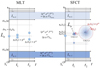Fig. 2.

Artistic representation of temporal evolution of a convective element. The star is a superposition of m layers in hydrostatic equilibrium. The generic layer, L_n, is defined by the hydrostatic pressure, density, and temperature (p,ρ,T)_{L_n}. These values are assumed to be time-independent and far away from the convective element, i.e., for every layer $(p^{\infty}, ρ^{\infty}, T^{\infty}) = {(p, ρ, T)}_{L_{n}} \forall t$ $\left( {{p}^{\infty }},{{\rho }^{\infty }},{{T}^{\infty }} \right)={{\left( p,\rho ,T \right)}_{{{L}_{n}}}}\forall t$ . Vice versa, each convective element is never in hydrostatic equilibrium with its medium, and the pressure, temperature, and density at the surface of a convective element are {p_e(t),ρ_e(t),T_e(t)}≠{p^∞,ρ^∞,T^∞}. Upper and lower borders of a layer are indicated by ∂L_n = ∂L_n(x). Data are from Pasetto et al. (2019).

In contrast, a self-consistent and coherent description of the temporal evolution of the pressure and motion of a convective eddy in relation to its independent coordinates is given by the SFCT proposed by Pasetto et al. (2014). This approach stems from a more general theory of the non-inertial linear instabilities of a gas, in which the Rayleigh-Taylor and Kelvin-Helmholtz instabilities are included. The SFCT assumes spherical symmetry for the convective eddy to simplify the mathematical formulation in the context of the potential-flow formalism. A description of the temporal and spatial pressure differences at the surface of a convective element with respect to the surrounding medium has already been investigated and presented by Pasetto et al. (2016) in the context of the SFCT. In that study (see their Fig. 1), the temporal evolution of the pressure at the surface is compared with the hydrostatic equilibrium pressure of the star. The description of the convective elements presented by Pasetto et al. (2014) and Pasetto et al. (2016) already takes the condition of non-hydrostatic equilibrium on the surface of a convective eddy into account in the definition of the latter and includes the dependence on time of this condition (unlike the case of the MLT).

4. Capturing the essence of the SFCT

Given the relevance of the pressure description inside a star, it is essential to highlight the implications of the pressure description adopted by the SFCT and to understand if the founding hypotheses of the SFCT can capture the behavior of a convective blob rolling up in fluid vortices.

4.1. SFCT limit cases: Eddies at rest

A basic assumption on which the SFCT stands is that the expansion or contraction rate of a convective element is much larger than the motion of its barycenter. In Fig. 2, this is artistically represented by the expansion of the radius, R, of the generic convective element, which is much larger than the vertical motion of this passing from the arbitrary time t₁ to t₂ > t₁. If we follow the expansion or contraction in the non-inertial reference S₁(O′,r), co-moving with the barycenter of the convective eddy at velocity v_O′ (relative to the inertial system S₀(O; t) whose origin is at the center of the star O), we can write $∥ {\dot{r}}_{e} ∥ = \dot{R} ≫ v_{O'}$ $\left\| \boldsymbol{\dot r }_{\mathrm{e}} \right\| = \dot R \gg {\mathit{v}_{O^\prime}}$ . Clearly, the assumption made here that eddies are at rest and that their motion is merely expansion or contraction refers to an ideal situation that does not correspond to reality and does not find counterparts in any hydrodynamical simulation. The case is only presented here to capture the main features of sole expansion (the novelty of the SFCT) as compared to the sole vertical motion (the situation of the MLT). This extreme approximation is possible thanks to the fact that eddies are supposed to die shortly after their birth and to dissolve through instabilities of a different kind (they are presented below), thus releasing their energy to the surrounding medium.

If the expanding or shrinking elements of the SFCT capture the essential behavior of physical eddies rolling up in turbulent vortices, then we should be able to achieve reasonably good results in the pressure description, even if we completely neglect their vertical motion. This means investigating the behavior of the SFCT in the limit case of a homogeneous-isotropic medium, a situation that can be easily achieved by nullifying the acceleration, that is, setting a_O′ = 0, in the core of Eq. (7) of the SFCT³. Since no translation of the convective elements is considered, this would be the case in which all the energy transport is carried by convective elements with little vertical motion but with large expansion, the opposite of what is supposed to occur with the MLT in which only the vertical motion is present. The scientific case we are investigating should be considered as a mathematical idealization meant to capture the essence of the role played by the sole expansion as compared to the case of the sole vertical motion.

The expansion of a convective element can be described with the formalism of the velocity-potential flow (e.g., Landau & Lifshitz 1959). In the following, we show that this simple description can capture the essence of the convective turbulence as already pointed out by Pasetto et al. (2014). In the absence of a translation of the convective element, we can simplify the formalism of Pasetto et al. (2014), making use of two reference frames moving relatively to each other to a single static one. It is convenient to simplify the notation S₁(O′,r) ≡ S₀(O,x)∀t. By assuming spherical coordinates in S₁, we write S₀(x) = S₀(r) = S_O(r,θ,ϕ). The system can be described simply by the evolution of the radius vector, ∥r∥ ≡ r, whose value at the surface of a convective element at the time t is ${∥ r ∥}_{e} {\hat{e}}_{r} = R (t)$ ${\left\| {\boldsymbol{r}} \right\|_{\mathrm{e}} }{\hat e_{\mathrm{r}}} = R(t)$ .

Under these assumptions, in S₀ the potential vector Φ_v₀ and velocity field v₀ are

$\begin{matrix} Φ_{v_{0}} = - \frac{\dot{R} R^{2}}{r} and v_{0} = \frac{\dot{R} R^{2}}{r^{2}} {\hat{e}}_{r}, \end{matrix}$ $\begin{aligned} {\Phi _{{{\boldsymbol{v}}_0}}} = - \frac{{\dot{R}{R^2}}}{r} \quad \mathrm{and} \quad {{\boldsymbol{v}}_0} = \frac{{\dot{R}{R^2}}}{{{r^2}}}{\hat{e}_{\rm r}}, \end{aligned}$

respectively. In consideration of these premises, at an arbitrary but fixed time t the Bernoulli equation in S_O reads as Eq. (6), and with

$\begin{matrix} {\begin{matrix} \frac{\partial Φ_{v_{0}}}{\partial t} = - \frac{R (2 {\dot{R}}^{2} + R \ddot{R})}{r} \\ \frac{{∥ v_{0} ∥}^{2}}{2} = \frac{1}{2} 〈 \frac{\partial Φ_{v_{0}}}{\partial r}, \frac{\partial Φ_{v_{0}}}{\partial r} 〉 = \frac{1}{2} \frac{R^{4} {\dot{R}}^{2}}{r^{4}}, \end{matrix} \end{matrix}$ $\begin{aligned} \left\{ \begin{array}{l} \frac{{\partial {\Phi _{{{\boldsymbol{v}}_0}}}}}{{\partial t}} = - \frac{{R\left( {2{{\dot{R}}^2} + R\ddot{R}} \right)}}{r} \\ \frac{{{{\left\Vert {{{\boldsymbol{v}}_0}} \right\Vert}^2}}}{2} = \frac{1}{2}\left\langle {\frac{{\partial {\Phi _{{{\boldsymbol{v}}_0}}}}}{{\partial r}},\frac{{\partial {\Phi _{{{\boldsymbol{v}}_0}}}}}{{\partial r}}} \right\rangle = \frac{1}{2}\frac{{{R^4}{{\dot{R}}^2}}}{{{r^4}}}, \\ \end{array} \right. \end{aligned}$ (36)

it becomes

$\begin{matrix} \frac{P (r ; t)}{ρ (r ; t)} + \frac{1}{2} \frac{R^{4} {\dot{R}}^{2}}{r^{4}} - \frac{R (2 {\dot{R}}^{2} + R \ddot{R})}{r} = const . \end{matrix}$ $\begin{aligned} \frac{{P\left( {r;t} \right)}}{{\rho \left( {r;t} \right)}} + \frac{1}{2}\frac{{{R^4}{{\dot{R}}^2}}}{{{r^4}}} - \frac{{R\left( {2{{\dot{R}}^2} + R\ddot{R}} \right)}}{r} = \mathrm{const}. \end{aligned}$ (37)

We set the constant by requiring P(∂L;t) = P^∞ and ρ(∂L;t) = ρ^∞ far away from the sphere for all t, mainly because the size L of the layer is much larger than that of the eddy (see Fig. 2). We note here that the formulation of the problem is fully general, not requiring the hydrostatic condition at the border of the domain of the definition ∂L. On the contrary, P(∂L;t) can be the value of any other pressure within L and outside the eddy without invalidating these arguments. This argument is implicit in the sharing of the pressure information introduced by Eq. (34), whose applicability is fully general. Nevertheless, we always assume that the stellar convective layer is always in rigorous hydrostatic equilibrium, i.e., SFCT correctly assumes hydrostatic equilibrium at ∂L for each L and each t. Therefore, with these considerations and relaxing the time dependence only in the density ρ, we can complete the physical description in Eq. (37) with

$\begin{matrix} \frac{P (r ; t)}{ρ} + \frac{1}{2} \frac{R^{4} {\dot{R}}^{2}}{r^{4}} - \frac{R (2 {\dot{R}}^{2} + R \ddot{R})}{r} = \frac{P^{\infty}}{ρ^{\infty}}, \end{matrix}$ $\begin{aligned} \frac{{P\left( {r;t} \right)}}{\rho } + \frac{1}{2}\frac{{{R^4}{{\dot{R}}^2}}}{{{r^4}}} - \frac{{R\left( {2{{\dot{R}}^2} + R\ddot{R}} \right)}}{r} = \frac{{{P^\infty }}}{\rho ^\infty }, \end{aligned}$ (38)

which simplifies as

$\begin{matrix} \frac{{\dot{R}}^{2}}{2} \frac{R^{4}}{r^{4}} - \frac{R}{r} (2 {\dot{R}}^{2} + R \ddot{R}) = \frac{P^{\infty} - P (r ; t)}{ρ^{\infty}} . \end{matrix}$ $\begin{aligned} \frac{{{{\dot{R}}^2}}}{2}\frac{{{R^4}}}{{{r^4}}} - \frac{R}{r}\left( {2{{\dot{R}}^2} + R\ddot{R}} \right) = \frac{{{P^\infty } - P\left( {r;t} \right)}}{\rho ^\infty }. \end{aligned}$ (39)

This is either a differential equation for R(t) if the pressure is given or an equation for the pressure field if R(t) is given. We followed this second interpretation because, from Eq. (B15) of Pasetto et al. (2016; see also Fig. A1 of Pasetto et al. 2014), we already learned that the interesting temporal evolution of the convective eddy is quadratic in time to the first order. This means that we assume the solutions of interest here are those of the type

$\begin{matrix} \frac{R}{R_{0}} = 1 + \frac{t^{2}}{t_{0}^{2}}, \end{matrix}$ $\begin{aligned} \frac{R}{{{R_0}}} = 1 + \frac{{{t^2}}}{{t_0^2}}, \end{aligned}$ (40)

and we solve Eq. (38) as an equation for the pressure field. We look at a generic sphere instantaneously overlapping the expanding eddy with R ∝ t², set r = R(t) in Eq. (39) and make use of Eq. (40) to obtain the following:

$\begin{matrix} {\frac{{\dot{R}}^{2}}{2} \frac{R^{4}}{r^{4}} - \frac{R}{r} (2 {\dot{R}}^{2} + R \ddot{R}) |}_{r = R} = {\frac{P^{\infty} - P (r ; t)}{ρ} |}_{P = P_{e}} \Leftrightarrow \\ \frac{1}{2} \frac{τ^{2} {(1 + τ)}^{8}}{χ^{4}} - \frac{{(1 + τ)}^{4}}{χ} (\frac{1}{2} + \frac{2 τ^{2}}{{(1 + τ)}^{2}}) = \frac{DP}{P^{\infty}}, \end{matrix}$ $\begin{aligned}&{\left. {\frac{{{{\dot{R}}^2}}}{2}\frac{{{R^4}}}{{{r^4}}} - \frac{R}{r}\left( {2{{\dot{R}}^2} + R\ddot{R}} \right)} \right|_{r = R}} = {\left. {\frac{{{P^\infty } - P\left( {r;t} \right)}}{\rho }} \right|_{P = {P_{\rm e}}}} \Leftrightarrow \nonumber \\&\frac{1}{2}\frac{{{\tau ^2}{{\left( {1 + \tau } \right)}^8}}}{{{\chi ^4}}} - \frac{{{{\left( {1 + \tau } \right)}^4}}}{\chi }\left( {\frac{1}{2} + \frac{{2{\tau ^2}}}{{{{\left( {1 + \tau } \right)}^2}}}} \right) = \frac{{DP}}{{{P^\infty }}}, \end{aligned}$ (41)

where, for the sake of simplicity, we set ${\frac{r}{R_{0}}, \frac{t}{t_{0}}} \equiv {χ, τ}$ $\left\{ {\frac{r}{{{R_0}}},\frac{t}{{{t_0}}}} \right\} \equiv \left\{ {\chi ,\tau } \right\}$ and achieve standard non-dimensionality of the partial differential equation by setting $\frac{ρ^{\infty}}{P^{\infty}} {(\frac{2 R_{0}}{t_{0}})}^{2} \equiv 1$ $\frac{\rho^\infty }{{{P^\infty }}}{\left( {\frac{{2{R_0}}}{{{t_0}}}} \right)^2} \equiv 1$ . With a similar procedure, the velocity field is

$\begin{matrix} \frac{v_{r}}{v_{0}} = \frac{2 τ {(1 + τ^{2})}^{2}}{χ^{2}}, \end{matrix}$ $\begin{aligned} \frac{{{{ v}_r}}}{{{{ v}_0}}} = \frac{{2\tau {{\left( {1 + {\tau ^2}} \right)}^2}}}{{{\chi ^2}}} ,\end{aligned}$ (42)

with $v_{0} \equiv \frac{R_{0}}{t_{0}}$ ${\mathit{v}_0} \equiv \frac{{{R_0}}}{{{t_0}}}$ . In this way, the expansion of the convective elements increases with time χ ∝ τ² while it is immediate to see that to the leading order (i.e., by series expansion to ∂L) the pressure difference, DP, drops with space but increases with time as DP ∝ τ² in compliance with the Bernoulli theorem. In particular, the following temporal relation holds:

$\begin{matrix} χ \propto τ^{2} \Rightarrow D P \propto τ^{2}, \end{matrix}$ $\begin{aligned} \chi \propto {\tau ^2} \Rightarrow DP \propto {\tau ^2}, \end{aligned}$ (43)

which correlates the temporal evolution of the pressure at the surface of a convective element to that of the surrounding medium as imposed and predicted by Eq. (31). To better clarify the results we obtained, in Figs. 3 and 4 we plot the temporal and spatial dependences of the pressure and velocity fields around the ideal convective elements as obtained in Eqs. (41) and (42).

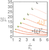Fig. 3.

Temporal and spatial evolution of relative pressure ratio between the value at the surface of a convective element and the one at infinity. Time runs from τ = 0 to τ = 2 from the bottom to the top. The lines start at the surface of a generic spherical element whose position and dimensions grow with time. The radius increases according to Eq. (40). The curves starting from the surface of the different spheres show the variation of the relative pressure difference moving far away from the surface of the element to large distances. The lines refer to the case of a fluid in the irrotational potential-flow approximation. The dashed line shows (limited to one case) the expected variation for a rotational flow. The disintegration of any generic convective element as time goes on is mimicked here by drawing the spheres and lines with progressively less intense colors. Data are taken from Pasetto et al. (2019).

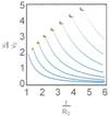Fig. 4.

Same as in Fig. 3, but for the velocity field surrounding the eddy. Data are taken from Pasetto et al. (2019).

In Fig. 3 the different lines represent the different temporal evolution of the pressure field. As time increases, the convective element grows in size, as given by Eq. (40) and represented by the 3D spheres. It is soon evident that not only is DP ≠ 0∀t, but it even grows with time, contradicting the widespread belief that DP = 0 (e.g., Eq. (6.2) in Kippenhahn et al. 2012). Only far away from the convective element does DP → 0. In such a case, however, this scheme (and SFCT) fails because each star has a finite size and lifetime, each layer of a star is of finite size, and computations concerning the layers of a star are meaningful only over a limited range of time. Since no hydrostatic equilibrium has been imposed in this example, P^∞ can be the pressure existing at the surface of any nearby element. For the sake of comparison, in Fig. 3 we also plot the spatial pressure dependence expected far away from the convective element in the case of a rotational medium (dashed line).

Similar considerations can be made for the velocity field surrounding a convective element as a function of time and position (see Fig. 4). We note that the velocity of any fluid element at any arbitrary location r, v_r = v_r(r;t) ≠ Ṙ everywhere apart from the instantaneous location of the sphere overlapping the element surface.

The scientific case we have just illustrated is useful when compared to the more complex treatment presented in Pasetto et al. (2014) and helps one to understand the meaning of the decoupled equations of motion presented in Eq. (3) of Pasetto et al. (2016) and reiterated in the previous section. A few points are worth highlighting: (i) The pressure gradients presented in this simple case show the same asymptotic trends displayed in the more complex, non-inertial treatment of moving convective elements used by Pasetto et al. (2014). At first glance, the ability of this simple exercise to capture the essence of the SFCT may be somewhat surprising only for the different formalism and the different physical content. The SFCT requires both the hypothesis of hydrostatic equilibrium to occur far away from the convective element and the condition $∥ \dot{R} ∥ ≫ v_{O^{'}}$ $\left\| {{{{\boldsymbol{\dot R }}}}} \right\| \gg {\mathit{v}_{O^\prime}}$ , otherwise the quadratic dependence of Eq. (43) is not formally met. Here, neither hypothesis is used, but the plot of Fig. 3 is very similar to that of Fig. 1 in Pasetto et al. (2016), where a similar trend was derived. (ii) The velocity field shown in Fig. 4 tells us that the longer the elapsed time, the more the convective element expands/contracts, and the less the approximation Dp = 0 holds. The relationship between the radial dimension and time for the generic convective element (see Eq. (40), above) can be compared to that of Eq. (B15) of Pasetto et al. (2016), which presents the same trend. (iii) The velocity-potential formalism describes the trend of pressure across the medium and does not affect the vertical motion. The decoupling of the independent coordinates demonstrated by Pasetto et al. (2016; their Eq. (3)) using independent arguments based on classical mechanics about translation and expansion of convective elements is here clarified by hydrodynamic arguments based on the Bernoulli equation (Eq. (6)). This strengthens the Corollary 1 in Sect. 4.2 of Pasetto et al. (2014); the hydrodynamics of a single stellar layer considered at constant acceleration is a good approximation as far as Eq. (34) is concerned. (iv) The temporal evolution of the pressure and the expansion of the convective elements are intimately related and cannot be separated without violating the energy conservation principle (i.e., the Bernoulli theorem). If we want to examine the expansion or contraction of the convective elements, we cannot ignore the time evolution of the pressure and vice versa. This is done coherently in the SFCT but not in the MLT. The MLT copes with its fundamental failure in describing the temporal evolution of the system by introducing a parameter that tacitly accounts for the conservation of the energy as a function of time. (v) It is important to remember that DP = 0 does not affect the derivation of the Schwarzschild (∇_rad < ∇_ad) and/or the Ledoux (∇_rad < ∇_ad + φδ/∇_μ) criteria for instability as already proved by Pasetto et al. (2014, Lemma 2).

To summarize, the consequence of Figs. 3 and 4 is that as the convective element expands, the pressure difference with respect to the surrounding medium pushes it further away from equilibrium rather than towards equilibrium. In this illustrative case in which there is no translational movement of the element, the increase in size driving this evolution is inserted by hand through Eq. (40), so there is no need to specify the energy source driving the whole process. In the complete treatment of Pasetto et al. (2014), which includes the movement of the bubble, this expansion is self-consistently derived, and it is effectively driven by the temperature gradients ∇ and ∇_e when a layer L becomes convective. We provide a test case of this situation in Sect. 6. Finally, while the eddy expands, instabilities set in and destroy it, as discussed in Sect. 4.3 below.

4.2. The danger of the instantaneous pressure adjustment

Failing to understand Eq. (34), whose original analysis dates back to the milestone studies of Batchelor & Proudman (1956) and Saffman (1967), as well as violating the energy conservation principle required by the Bernoulli equation, can lead to bizarre results, as in the study by Miller Bertolami et al. (2016) on which we want to comment here. While in the MLT, the fundamental relation of Eq. (34) is implicitly hidden through the parameter Λ_m, it was explicitly ignored by Miller Bertolami et al. (2016). In light of the work reviewed in Sect. 1 and the exemplification in Sect. 4, the analysis of the potential-vector approximation presented by Miller Bertolami et al. (2016) is incorrect for three reasons.

The authors assume instantaneous hydrostatic equilibrium (i). This is evident in the derivation of their Eq. (2). It does not contain any free parameter, such as the ML, to compensate for the violation of the basic relationship of Eq. (34). The authors write

$\begin{matrix} \frac{d P (r ; t)}{d t} = \frac{d P (r)}{d r} v_{b} (t), \end{matrix}$ $\begin{aligned} \frac{{\mathrm{d}P\left( {{\boldsymbol{ r }};t} \right)}}{{\mathrm{d}t}} = \frac{{\mathrm{d}P\left( {\boldsymbol{ r }} \right)}}{{\mathrm{d}r}}{{ v}_{\rm b}}\left( t \right), \end{aligned}$

so that for v_b(t) = 0, i.e., a bubble at rest, one has

$\begin{matrix} \frac{d P (r ; t)}{d t} = 0 \Leftrightarrow P (r ; t) = P (\infty ; t) = const . \end{matrix}$ $\begin{aligned} \frac{{\mathrm{d}P\left( {{\boldsymbol{ r }};t} \right)}}{{\mathrm{d}t}} = 0 \Leftrightarrow P\left( {{\boldsymbol{ r }};t} \right) = P\left( {\infty ;t} \right) = \mathrm{const}. \end{aligned}$

However, this contradicts Eq. (34), which shows how the pressure at the surface of an element and at infinity is never the same. Their approach leads them to their Eq. (8), which has no regime of validity to our knowledge. Later, using their Eq. (A6), Miller Bertolami et al. (2016) claim that a convective element and medium have almost the same pressure. As discussed in Sect. 4, this is never the case, and it is more strikingly evident from Fig. 3, where convective elements and media have approximately the same pressure only for short times (say τ ≤ 1) and depart from each other as time increases. It is worth noting here that Fig. 3 refers to the exercise of Sect. 4. To obtain the correct numerical values for densities, temperatures, times, and so on, the layer under examination should be inserted in a real environment with the EoS of a star. This was already shown in Fig. 1 of Pasetto et al. (2016) and for brevity is not repeated here. No equilibrium can exist for a convective element coming into existence (ii). The authors assumed instantaneous adjustment of the pressure equilibrium (see their Eq. (8)), that is, Miller Bertolami et al. (2016) did not take into account the time and space evolution of pressure, but at the same time they followed the temporal evolution of the size of a convective element (one of the degrees of freedom of the system) in S_O, ∥x_e(t)∥, and at the same time the motion of x_O(t) (the other degree of freedom), which is mathematically and physically inconsistent. No turbulence can exist if the pressure adjusts itself instantaneously (iii); the pressure waves caused by the pressure fluctuations at a given eddy position are the trigger for the formation of other eddies and give rise to turbulent convection. While SFCT captures the fundamentals of this process, it is missing from Miller Bertolami et al. (2016, see, e.g., their result in Eq. (A6)).

The most obvious drawback in the theory of Miller Bertolami et al. (2016) becomes clear looking at our Eq. (43) (repeated here for the sake of clarity),

$\begin{matrix} χ \propto τ^{2} \Rightarrow D P \propto τ^{2}, \end{matrix}$ $\begin{aligned} \chi \propto {\tau ^2} \Rightarrow DP \propto {\tau ^2}, \end{aligned}$ (44)

at the surface of the convective element. Contrary to what is obtained here in compliance with the physics expressed by Eq. (34), Miller Bertolami et al. (2016) derived their Eq. (A6), (backbone of their Eq. (2) and the rest of the paper), which predicts the opposite of Eq. (44). The authors failed to investigate the limit of their Eq. (A6), because they computed the limit of P = P(r,t) without examining whether the bubble itself can exist in that regime both in time and space. We have shown here that if Bernoulli’s theorem is correctly fulfilled (and hence the energy conservation principle), it cannot be that P^∞ ≃ P anywhere and anytime. Coherently, the velocity field shown in Fig. 4 tells us that the longer the elapsed time, the more the convective element expands or contracts, the less the approximation of Eq. (A6) in Miller Bertolami et al. (2016) holds. Indeed, the correct physical formulation and analysis of the whole problem impose the pressure-time dependence of Eq. (43). In particular, even far away from the element, the condition P^∞ ≃ P cannot happen because of the temporal divergence in the equations (in any case, as time increases, the convective elements are destroyed by instabilities, as examined in Pasetto et al. 2016).

4.3. The fate of a convective element

Finally, we examine the fate of an expanding/contracting convective element. As already mentioned in Pasetto et al. (2016), the SFCT fails in compressible regimes and in the very external layers of a star where suitable boundary conditions must be supplied (see below). In addition to it, the current formulation of the SFCT does not consider that convective elements cease to exist at t → ∞. Several instabilities concur to dissipate and destroy the elements after a finite lifetime. Possible physical causes of disintegration include deformation, whereby the convective elements dissolve, losing their initial spherical geometry. This mirrors the classical picture of a turbulent eddy that winds up in vortex sheets in a sequence of azimuthal vorticity and poloidal motions and sweeps angular momentum outward radially to form sheets. The start of this process is captured by the linear treatment in terms of a stability parameter named $γ_{I}^{2}$ $\gamma _I^2$ function of position and time (e.g., Plesset 1954, and references). Secondly, we have the Rayleigh–Taylor instability, that is, the finger-like penetration of two fluids at different densities (e.g., a convective element expanding inside a radiative or convective fluid). The process depends on (i) the density difference between the two fluids; the instability parameter $γ_{RT}^{2}$ $\gamma_{\rm RT}^2$ and (ii) the relative acceleration between the two fluids with instability parameter $γ_{a - RT}^{2}$ $\gamma_{a - {\rm RT}}^2$ . Both parameters are functions of position and time (see Pasetto et al. 2019 for more details). Finally, there is, the Kelvin–Helmholtz instability (i.e., the relative sliding of the inner layers with respect to the external ones of convective elements) helping to dissolve the convective elements themselves. The instability parameter $γ_{KH}^{2}$ $\gamma_{\rm KH}^2$ is a function of position and time. At the first order, no dependence on the acceleration of the convective element is found. We invite the reader to consult Pasetto et al. (2016) for an extensive investigation and Pasetto et al. (2019) for more details.

5. Boundary conditions and stellar models with the SFCT

The SFCT is fully dynamical, i.e., it explicitly includes the time. In the very external layers, convective elements cannot travel and expand upward beyond the star’s surface. This limit dramatically reduces the dimension, velocity, and lifetime of elements that come into existence close to the star’s surface. Therefore, close to the surface the maximum time allowed to an element can be shorter than the time needed to reach the asymptotic value for v. Consequently, the expressions for ∇ and ∇_e must take this fact into account. Special care has to be paid not to blindly apply the theory where it may lose physical significance, i.e., when the time to disposal does not allow convection to reach the “asymptotic regime”.

5.1. Simple boundary conditions

Based on these ideas, Pasetto et al. (2016) proposed that suitable boundary conditions should accompany the SFCT at the surface layers. It is worth recalling that the outer layers’ physical structure and the star’s effective temperature are dominated by the role played by convection in the atmosphere, while the luminosity, which is essentially built up deeper in the interiors, is much less affected by this. The starting point of their analysis is the definition of two characteristic times: (i) t_asy, i.e., the time at which the solution of the quintic equation satisfies all the constraints set by the conditions of Eq. (27) with Π = 0.98. It is worth noting that different values of Π fixed arbitrarily give different t_asy; and (ii) t_cnv, that is, the timescale needed by any perturbation taking place inside a convective region of width ΔW_cnv to propagate across the whole region owing to continuous upward or downward motion of the fluid elements. The maximum possible speed for this to occur is the sound speed $v_{s} = \sqrt{Γ_{1} P / ρ}$ $\mathit{v}_{\mathrm{s}}= \sqrt{\Gamma_1 P/\rho}$ , where Γ₁ is the generalized adiabatic exponent including the effect of radiation pressure and ionization (Cox & Giuli 1968). In the SFCT, a convective element moves radially with velocity v_e and expands its dimension at the rate $\dot{ξ_{e}}$ $\dot {\xi_{\mathrm{e}}}$ . Since the maximum increase of dimensions attainable by a convective element Δξ_e can be expressed as a fraction of the extension of a convective region ΔW_cnv, i.e., Δξ_e → ηΔW_cnv, t_cnv is approximately

$\begin{matrix} t_{cnv} ≃ \frac{Δ ξ_{e}}{{\dot{ξ}}_{e}} ≃ \frac{Δ ξ_{e}}{v_{s}} ≃ η \frac{Δ W_{cnv}}{v_{s}} . \end{matrix}$ $\begin{aligned} {t_{{\text{ cnv}}}} \simeq \frac{{\Delta {{ \xi }_{\rm e}}}}{{{{\dot{\xi }}_{\rm e}}}} \simeq \frac{{\Delta {{ \xi }_{\rm e}}}}{{{{ v}_{\rm s}}}} \simeq \eta \frac{\Delta W_{\rm cnv}}{ { v}_{\rm s}}. \end{aligned}$ (45)

In this relation, both the width ΔW_cnv of the convective region and the fraction η are not known a priori. A possible way out is to adopt an iterative technique (Pasetto et al. 2016); given a guess estimate for the product ηΔW_cnv, the whole procedure described in this section is iterated until the solution (v_e and $\dot{ξ_{e}}$ $\dot {\xi_{\mathrm{e}}}$ ) becomes constant with time and iteration. Numerical tests show that one or two iterations are enough to fix the solution.

At any layer, the asymptotic regime cannot be reached if the two timescales are in the

$\begin{matrix} \frac{t_{asy}}{t_{cnv}} = Π < 1, \end{matrix}$ $\begin{aligned} { \frac{t_{\rm asy}}{t_{\rm cnv}}} = \Pi < 1, \end{aligned}$ (46)

ratio, which is also another definition of Π. The condition (46) also fixes the maximum fraction of the local velocity with respect to its asymptotic value v_e(t_asy) reached in each layer:

$\begin{matrix} v_{e} = Π \times v_{e} (t_{asy}) . \end{matrix}$ $\begin{aligned} { v}_{\rm e} = \Pi \times { v}_{\rm e}(t_{\rm asy}). \end{aligned}$ (47)

The percentage Π now varies with the position. The typical run of the ratio Π, lifetime t_asy, and lifetime t_cnv as a function of log P in the most external layers of the atmospheric convection of a star is shown in the left and right panels of Fig. 5, respectively. The sudden fall off of Π and t_asy and the presence of the companion minimum is due to the fall off of the adiabatic gradient caused by the ionization of light elements such as H and He. The minimum of t_asy also coincides with the minimum in the acceleration of convective elements, and it occurs at the layer at which the dimension of a typical convective element is equal to the distance of this layer from the surface of the star; see Pasetto et al. (2016) for more details.

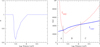Fig. 5.

Run of Π and characteristic timescales of convection in the most external layers of a low-mass star. Left panel: profile of Π across the atmosphere of the MS model of the 1.0 M_⊙ star with chemical composition [X = 0.703, Y = 0.280, Z = 0.017]. We note the fall of Π to the minimum value followed by the rapid increase to Π = 1 at increasing pressure. Right panel: run of the asymptotic time t_asy and convective time t_cnv as a function of log P in the atmosphere of the 1.0 M_⊙ at the Sun’s position (log L/L_⊙ = 0 and log T_eff = 3.762). The asymptotic time has a minimum at the position log P ≃ 5.4, roughly coincident with the adiabatic fall layer. This trend is the remote cause of the minimum in the ratio Π of the left panel, and it is related to the mathematical behavior of the real solutions of the quintic equation in the outermost layer of the external convection (see Fig. 3 of Pasetto et al. 2016). Data are from Pasetto et al. (2016).

Typical profiles of velocity and temperature gradients in the most external convective zone for the 1.0 M_⊙ star with chemical composition [X = 0.703, Y = 0.280, Z = 0.017] at the Sun’s position (log L/L_⊙ = 0 and log T_eff = 3.762) are shown in Fig. 6. Three cases are shown: models with the standard MLT (black lines), models with the SFCT and the boundary condition with Π = const (blue lines), and models with Π variable according to the position (red lines). In the following, the boundary conditions described in this section are indicated as “old boundary conditions”.

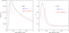Fig. 6.

Velocity and temperature gradients in SFCT stellar models with the old boundary conditions of Pasetto et al. (2016). Left panel: profile of the convective velocity as function of the pressure across the atmosphere of the 1.0 M_⊙ star with chemical composition [X = 0.703, Y = 0.280, Z = 0.017] at the Sun’s position (log L/L_⊙ = 0 and log T_eff = 3.762). The new boundary conditions are applied for log P ≤ 6.0. Three profiles are shown: the one from the MLT (black line), the one from the SFCT with the new boundary conditions (red dashed lines), and the one from the SFCT with the old boundary conditions (blue dotted line). Right panel: same as left panel, but for temperature gradient of the medium, ∇. Data are from Pasetto et al. (2016).

Based on these results, evolutionary sequences in which the external convection is calculated with SFCT integrated by condition (46) have been generated and compared with the correspondent ones based on the MLT (Pasetto et al. 2016). The new evolutionary sequences obtained from the SFCT match the corresponding sequences based on the MLT, whose ML parameter was calibrated on the Sun. This is shown by the path on the HRD of the 0.8, 1.0, 1.5, 2.0, and 2.5 M_⊙ stars displayed in Fig. 7, where the black crosses indicate the sequences with the MLT and the solid thick lines of different colors those with the SFCT.

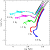Fig. 7.

Evolutionary tracks of 0.8, 1.0, 1.5, 2.0, and 2.5 M_⊙ stars calculated with the MLT (mixing length parameter Λ = 1.68) indicated by crosses and the SFCT indicated by the solid lines of different colors. The comparison shows that the SFCT with no mixing length parameter is equivalent to the classical MLT with calibrated mixing length parameter. Data are from Pasetto et al. (2016).

In general the paths on the HRD of models of the same mass but calculated with the calibrated MLT or the SFCT agree with each other. They are indeed indistinguishable from the zero-age main sequence up to the bottom of the RGB, while along the RGB at given luminosity the SFCT models are cooler than the correspondent ones calculated with the MLT. The effect tends to increase with the luminosity. This is a crucial point in relation to the interpretation of the observational data for old globular clusters where the RGBs are well defined. Unfortunately, the slope of the RGB does not only depend on the efficiency of external convection (mixing length parameter in the classical MLT), but also on the opacity and details of the chemical composition that in part mask the effect of convection. The issue surely requires future investigation that is beyond the aims of this study.

However, despite the success of the stellar models calculated by Pasetto et al. (2016) with the SFCT, we consider it wise to improve upon the boundary conditions they adopted for the following reasons. (i) The fact that the outermost layers also have Π = 1 has been ignored. (ii) The velocity profiles in the region 5 < log P < 6 dyn cm⁻² of the SFCT very much deviates from that of the MLT. (iii) Equally, for the ∇ profile in the same pressure interval, the peak value of ∇ occurs at a different pressure in the two theories. Since what happens in these outermost regions is of paramount importance, we are convinced that further investigation of the behavior of external convection and companion boundary conditions is needed.

5.2. Revision of the boundary conditions

We recognize that the straightforward layer-by-layer solution of the quintic equation using the condition Π = 1 usually yields velocities comparable to and gradients ∇s significantly smaller than those obtained from the classical MLT. Consequently, the associated stellar models are too blue on the HRD compared to those from the MLT. The opposite happens if the velocities and temperature gradients are lower and higher, respectively. In the alternative, using variable Πs as shown in the right panel of Fig. 5, the effective temperatures from the two theories are virtually identical (it is worth recalling that the luminosities of correspondent models are the same independently from the convection theory in use), and the paths of stellar models of given masses are virtually indistinguishable. However, the detailed profiles of v and ∇ in the outermost region of a star are significantly different. To define the causes of such an odd situation and to highlight the physical meaning of the boundary conditions, we carried out the following analysis in several steps:

The first step involves the heuristic 𝔉 function. It is inspired by the MLT study of Magic (2016), which derived the 𝔉 function defined by

$\begin{matrix} F = \frac{\nabla}{\nabla_{ad}}, \end{matrix}$ $\begin{aligned} \mathfrak{F} = \frac{\nabla }{\nabla _{\rm ad} }, \end{aligned}$ (48)

the factor by which the local value of the adiabatic gradient has to be multiplied to obtain the ambient gradient able to generate the correct effective temperature of the model. This analysis stands on the STAGGER grid of 3D stellar atmosphere models by Magic et al. (2013a,c). Although the models by Magic (2016) should not be used for stellar models above 1.4 M_⊙ (see the remarks made by Kochukhov et al. 2007), but they can be used for exploratory purposes. Well aware of the intrinsic limits of this analysis, we computed the 𝔉 function for a 1.0 M_⊙ star calculated with the MLT, for which we already know the path on the HRD. The resulting 𝔉 function is shown in the left panel of Fig. 8. As a function of log P (the position in the atmosphere), the 𝔉 function significantly decreases in the 5.4 ≤ log P ≤ 6.0 dyn cm⁻² interval, and it is nearly constant elsewhere: ⟨𝔉⟩≃1.6 for log P < 5.4 dyn cm⁻² and ⟨𝔉⟩≃1.0 for log P > 6.0 dyn cm⁻². In the course of evolution, the 𝔉 function extends more and more to lower values of the pressure because the star expands while moving along its path on the HRD (we consider here only the first movement from the main sequence to the RGB). Once the 𝔉 function is known, another sequence of stellar models with the same mass is calculated in which the ambient temperature gradient ∇ is directly derived from the 𝔉 function without passing through the MLT. As expected, the two sequences are identical. The great surprise comes when the same 𝔉 function is applied to calculate evolutionary sequences of different masses. Here, the test has been applied to stars in the mass range of 0.8–1.5 M_⊙: layer by layer, their adiabatic gradient ∇_ad is multiplied by 𝔉 function to obtain the ambient gradient ∇ and the evolutionary models in turn. The stellar tracks so calculated are in good agreement with those obtained from the full application of the MLT. This means that the 𝔉 function has much deeper physical significance than a simple way of expressing the ambient gradient using the adiabatic gradient. The 𝔉 function likely mirrors a fundamental property of invariance and self-similarity of stellar convection (see Magic 2016).

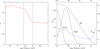Fig. 8.

Profiles of 𝔉 function, adiabatic temperature gradient ∇_ad, and ionization degrees of HI, HeI, and HeII in the external regions of a low-mass star. Left panel: profile of the 𝔉 function as a function of log P in the outer atmospheres of the 1.0 M_⊙ with chemical composition [X = 0.703, Y = 0.280, Z = 0.017] calculated with the MLT from the main sequence to late stages along the RGB. The adopted mixing length parameter is Λ = 1.68. The pressure is in dyn cm⁻². We highlight the two characteristic layers at log P = 5.4 and log P ≃ 6.0, where the 𝔉 function suddenly changes slope (see the text for more details). Right panel: run of adiabatic temperature gradient ∇_ad and ionization degree of HI, HeI, and HeII indicated by y_HI, y_HeI, and y_HeII, respectively, as a function of log P in dyn cm⁻². The drop off of ∇_ad at log P ≃ 5.4 coincides with the start of the HI ionization.

This suggests we should take the 𝔉 function as an important foundation of the external convection with particular attention to the two layers where the function 𝔉 changes slope, that is, log P ≃ 5.4 dyn cm⁻² and log P ≃ 6.0 dyn cm⁻². In any case, except for these general considerations and the few exploratory stellar models we calculated, no other use of the 𝔉 function exists in this study.

Secondly, we have the adiabatic fall. The low values of pressure in the above interval immediately suggest that all this occurs in regions in which ionization begins and the adiabatic temperature gradient drops from the ∇_ad = 0.4 typical of a neutral, perfect gas with negligible radiation pressure to much lower values when H and He start being ionized. The situation is shown in the right panel of Fig. 8 for the atmosphere of our 1.0 M_⊙ star representing the Sun. Ionization of H begins at log P ≃ 5.5 dyn cm⁻² and when the ionization degree is y_H ≃ 0.15, ∇_ad reaches its minimum (log P ≃ 6.0 dyn cm⁻²). These results are identical to those shown in the textbook by Kippenhahn & Weigert (1994, their Fig. 14.1, p. 114). This indirectly confirms the quality and accuracy of the calculations of key thermodynamical quantities in the atmospheres of the stellar models in use. This entire region, and the layer at log P ≃ 5.5 dyn cm⁻² in particular, will turn out to be of paramount importance in our analysis. We name this layer the “adiabatic fall”. It might be useful to recall here that the adiabatic fall simply mirrors the change in the degrees of freedom of the gas passing from neutral to a mixture of partly ionized atoms and free electrons.

Thirdly, we have times t_asy and t_cnv. It is worth looking again at the spatial variation of the asymptotic time t_asy evaluated using Π = 1 everywhere plotted in the right panel of Fig. 5 (solid red line). Going inward, the asymptotic time first rapidly decreases, reaches a minimum value, and then steadily increases. Remarkably, the layer of minimum t_asy occurs at the same pressure at which the layer of the adiabatic fall and, even more importantly, the minimum of the ratio Π (see Fig. 5) are located. The minimum value is about 2000 s. The trend of t_asy and the minimum value are related to the mathematical behavior of the real solutions of the quintic equation in the outermost layer of the atmospheric convection (see the discussion in Pasetto et al. 2016, Fig. 3). This trend is also the cause of the minimum in the ratio Π of Fig. 5, whereas the condition Π < 1 expressed by Eq. (46) is more effective in the branch rising from the minimum to Π = 1 above log P = 6.0 dyn cm⁻². In the right panel of Fig. 5, we also plot the time t_cnv (blue dotted line). In the pressure interval 5.4 ≤ log P ≤ 6.0 dyn cm⁻², t_cnv > t_asy, and therefore Π < 1. Above the pressure boundary log P = 6.0, Π = 1 as expected. However, for log P < 5.4 dyn cm⁻², t_asy > t_cnv and Π = 1 again. Since t_asy is longer than t_cnv in this region, the odd behavior of ∇ (abrupt change of slope when Π drops from 1 to the minimum value) in the right panel of Fig. 6 can be explained and ruled out. All this strengthens the idea that the layer of the adiabatic fall plays an important role in setting the right solution of the whole problem. As a general remark, we point out that since t_cnv increases smoothly and at a much smaller rate than the change of t_asy, the coincidence of the minimum of Π and the minimum of t_asy is expected to occur at the adiabatic fall, because in the super-adiabatic peak the buoyancy driving is the strongest. This coincidence can be considered as a test of self-consistency of the model.

Next, we have recasting the ratio Π. Starting from the given considerations, we recast the ratio Π in a different way. To this aim, we remind the reader of (i) the definition of the sound velocity v_s; (ii) the typical size of a convective region ΔW_cnv that can be expressed as function of the local pressure scale height h_p as ΔW_cnv = N × h_p, where N is a suitable number (in general ≫1, say about 200 from numerical calculations of stellar atmospheres) subject to change with the model, iteration, accuracy, and so on; (iii) the definition of pressure scale height h_p = P/(ρg); (iv) the expression for Γ₁ ≃ γχ_ρ with γ = c_p/c_v and χ_ρ = (∂lnP/∂lnρ)_t (see Cox & Giuli 1968 for details). The ratio Π of Eq. (46) becomes

$\begin{matrix} Π = t_{asy} (\frac{1}{v_{s}}) (\frac{g γ χ_{ρ}}{N}) . \end{matrix}$ $\begin{aligned} \Pi = t_{\rm asy} \left(\frac{1}{{ v}_{\rm s}}\right) \left(\frac{g \gamma \chi _\rho }{ N}\right). \end{aligned}$ (49)

The last term of the above relation is the local gravitational acceleration scaled by a numerical factor (always ≪1). This acceleration can be compared with the acceleration of the radial movement of a convective element according to the SFCT of Pasetto et al. (2014).

For the purposes of this analysis, it is sufficient to use the approximation of the acceleration given by Eq. (20) at the leading order in $\frac{h_{p}}{Δ r} \to \infty$ $\frac{{{h_{\mathrm{p}}}}}{{\Delta r}} \to \infty$ , in a chemically homogeneous convective layer. This is given by Eq. (22), which represents the acceleration of a convective element in the linear regime and recovers a well-known result of the MLT. Adapted to the present notation, it becomes

$\begin{matrix} A = g \frac{2 χ_{ρ}}{3} (\nabla - \nabla_{e}) \frac{Δ R}{h_{p}}, \end{matrix}$ $\begin{aligned} A= g \frac{2 \chi _{\rho }}{3} (\nabla -\nabla _{\rm e})\frac{\Delta R}{h_{\rm p}} , \end{aligned}$ (50)

where ΔR is the path traveled by a convective element during t_asy or the fraction of it that is compatible with the physical conditions of the surrounding medium, that is, if the local value of Π is < 1.

In the outer layers, sinking into the star t_asy first decreases to a minimum at the adiabatic fall and then rises again whereas t_cnv always increases inwards. Therefore, in the pressure interval 5.3 ≤ log P ≤ 6.1 dyn cm⁻², Π < 1, and consequently only a fraction of t_asy is made available to convective elements to grow in size and velocity. In addition to this, the mean size of convective elements ξ_e first decreases as long as the adiabatic fall layer is reached, and mildly increases afterwards. This would soon imply that the acceleration of convective elements decreases going from the surface to the critical layer and increases afterwards. The situation is shown in Fig. 9 where the left and right panels display the variation of ξ_e and acceleration A in cm s⁻² as function of log P, respectively. Both decrease moving from the surface to the adiabatic fall.

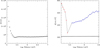Fig. 9.

Profiles of dimensions and acceleration of convective elements across the most external convective region of a low mass star. Left panel: dimension reached by the convective elements at t_asy as a function of log P. Since t_asy decreases, the velocity and dimensions of the convective elements in these very external layers are also expected to decrease going toward the adiabatic fall layer. Right panel: radial acceleration of a convective element as a function of the depth (log P) across the external convective zone of the stellar models representing the Sun (thin solid lines with triangles). With respect to the layer of the adiabatic fall (at log P = 5.4 dyn cm⁻²), the left branch of the curve (red triangles) is for ξ_e > D, i.e., Eq. (51), whereas the right branch (blue triangles) is for ξ_e < D, i.e., Eq. (52), and the minimum of the acceleration “coincides” with the value of ≃300 cm s⁻² given by the SFCT, see Eq. (50). The horizontal dotted line is the nearly constant acceleration from the MLT.

However, the fact that ξ_e does not increase as a function of the depth (or increases too little past the adiabatic fall) is a point of uncertainty and contradiction with numerical simulations of solar convection (see Stein & Nordlund 2000; Käpylä 2019). In relation to this, Canuto & Mazzitelli (1991, 1992) used the vertical density stratification to argue in favor of the growth of convective elements with the depth. Another point of weakness is the unexpected behavior of the large value of ξ_e at the surface of the convective zone. All this should be improved by the new boundary conditions proposed in this section.

Furthermore, in the SFCT the expansion rate of the convective element is larger than the displacement velocity (see condition (12) in Pasetto et al. 2014 or Appendix B2.3 in Pasetto et al. 2016). This implies that the increase of the radial position of the element ΔR can be only a fraction of ξ_e, i.e., ΔR = βξ_e, where β is unknown. If β ∼ 0.5 the local gravitational acceleration and the expansion accelerations at minimum of Π turn out to be equal and both amounting to ≃300 cm s⁻², as can be seen in the right panel of Fig. 10. Other values of β are possible and they must be determined by the iteration procedure used to determine v_e and ξ_e.

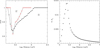Fig. 10.

Profiles of Π, Π′, and difference ∇ − ∇_e across the most external convective regions of a low-mass star. Left panel: ratios Π and Π′ are compared and found in good qualitative agreement. Right panel: difference ∇ − ∇_e as a function of position (log P). The maximum difference between the two gradients occurs at the layer of the adiabatic fall.

Another important point to note is that the layer at which the ratio Π is minimum coincides with the layer at which the radius of the average convective element ξ_e is equal to the distance D from the stellar surface, i.e., ξ_e/D = 1. For the outer layers, ξ_e > D, and for inner layers, ξ_e < D. It corresponds to the minimum possible value of the acceleration toward the surface and consequently to the maximum in the difference ∇ − ∇_e, and the minimum in the asymptotic time. The situation is illustrated in Fig. 10, where the left panel is for the acceleration, the mid panel for the ratio Π, and the right panel for the difference ∇ − ∇_e. The behavior of the acceleration as a function of the position can also be understood by considering that above the adiabatic-fall layer, where ξ_e > D, on the time interval t_asy the convective element has been able to grow to the dimension ξ_e and simultaneously to travel over a distance ΔR = βξ_e. Since ξ_e decreases here, the acceleration must decrease too. Below this layer, where ξ_e < D, the maximum path that a convective element can travel is D, and the acceleration can increase.

In order to better highlight the physical meaning of the ratio Π, we define a similar ratio making use of the acceleration of the radial movement of the convective elements given by Eq. (50) and replace the path ΔR with βξ_e in the extreme outer layers where ξ_e > D, and with D in the inner layers where ξ_e > D. The new ratio is named Π′. The two branches of Π′ above and below the layer ξ_e = D are

$\begin{matrix} Π^{'} = t_{asy} g \frac{2 χ_{ρ}}{3} (\nabla - \nabla_{e}) \frac{β ξ_{e}}{h_{p} v_{s}} for ξ_{e} > D, \end{matrix}$ $\begin{aligned}&\Pi^\prime =t_{\rm asy} \quad g \frac{2 \chi _{\rho }}{3} (\nabla -\nabla _{\rm e})\frac{\beta \xi _{\rm e}}{ h_{\rm p} { v}_{\rm s}} \quad \mathrm{for} \quad \xi _{\rm e}>D, \end{aligned}$ (51)

$\begin{matrix} Π^{'} = t_{asy} g \frac{2 χ_{ρ}}{3} (\nabla - \nabla_{e}) \frac{D}{h_{p} v_{s}} for ξ_{e} < D . \end{matrix}$ $\begin{aligned}&\Pi^\prime =t_{\rm asy} \quad g \frac{2 \chi _{\rho }}{3} (\nabla -\nabla _{\rm e})\frac{D }{ h_{\rm p} { v}_{\rm s}} \quad \mathrm{for} \quad \xi _{\rm e} < D . \end{aligned}$ (52)

The ratios Π and Π′ are not exactly the same, but their trend as a function of the position is similar. Furthermore, the transition between the two regimes (ξ_e > D and ξ_e < D) is not sharp, and a combination of the two formulas should be used. We are mostly interested in the value of Π′ and Π at the adiabatic fall layer, because what happens there drives the surface temperature gradients and the effective temperature of the atmosphere in turn (see the right panel of Fig. 10). Finally, it is worth clarifying that when the boundary conditions are applied to real stellar models, we use the ratio Π and not Π′. This latter is introduced only to highlight the physical meaning of the ratio Π.

Finally, we have the prescription for the new boundary conditions. We propose the following prescription. Looking at the right panel of Fig. 5, three different intervals of pressure can be defined. Firstly, in Region A t_asy/t_cnv > 1, and therefore according to condition (46) Π should be set equal to the maximum value Π = 1. However, this is not correct, because in this region ξ_e could easily exceed the distance D from the layer under consideration to the surface, which is not possible. Therefore, it is better to constrain the solution of the quintic equation to obey the logical sequence

$\begin{matrix} v_{e} \Rightarrow ξ_{e} = \frac{v_{e}}{2} \sqrt{χ} \Rightarrow ξ_{e} > D \Rightarrow ξ_{e} = D . \end{matrix}$ $\begin{aligned} { v}_{\rm e} \Rightarrow \xi _{\rm e} = \frac{{ v}_{\rm e}}{2} \sqrt{\chi } \Rightarrow { \xi _{\rm e} } > D \Rightarrow {\xi _{\rm e} = D}. \end{aligned}$ (53)

Therefore, velocity and integration time τ are fixed by the stage when the whole sequence starts being violated; the dimension of the convective element ξ_e is assumed equal to D. With these values for v_e and τ, we calculate the ambient temperature gradient ∇. The results for v_e (left panel) and ∇ (right panel) are shown in Fig. 10 and compared with the analogous value from the MLT for the case of the 1.0 M_⊙ best representing the Sun on the HRD.

Region B is similar to case A; however, now t_asy < t_cnv, and therefore Π < 1. As far as ξ_e is concerned, two regimes are found. Moving toward increasing pressure, t_asy first decreases to the minimum value and then increases again. The same goes for ξ_e, which is ξ_e > D before the minimum and then ξ_e < D past the minimum. In this region we adopt the following prescription. First, we derive the velocity at the asymptotic time t_asy. Let us call it v_e(t_asy). Then, we scale it to the value v_e = Πv_e(t_asy) < v_e(t_asy). The corresponding time is τ = t_asy/Π. This stems from the proportionality v_e(t_asy):t_asy = v_e(τ):τ. Above the layer of the minimum, the corresponding ξ_e could be wider than D. In this case, it is set as equal to D. Conversely, below the minimum, ξ_e < D, and the above limit does not apply. There are two logical sequences and types of constraint at work:

$\begin{matrix} t_{asy}, v_{e} (t_{asy}) \Rightarrow \\ v_{e} = Π v_{e} (t_{asy}), τ = t_{asy} / Π, ξ_{e} = D \\ v_{e} = Π v_{e} (t_{asy}), τ = t_{asy} / Π, ξ_{e} = \frac{v_{e}}{2} \sqrt{χ} . \end{matrix}$ $\begin{aligned}&t_{\rm asy}, { v}_{\rm e}(t_{\rm asy}) \quad \Rightarrow \nonumber \\&{ v}_{\rm e} = \Pi { v}_{\rm e}(t_{\rm asy}), \quad \tau = t_{\rm asy} / \Pi , \qquad \xi _{\rm e} = D \nonumber \\&{ v}_{\rm e} = \Pi { v}_{\rm e}(t_{\rm asy}), \quad \tau = t_{\rm asy} / \Pi , \qquad \xi _{\rm e} = \frac{{ v}_{\rm e}}{2} \sqrt{\chi }. \end{aligned}$ (54)

The resulting velocities and gradients are shown in Fig. 10.

Region C is the simplest case to treat, because now t_asy is always longer than t_cnv, so a maximum of Π = 1 holds everywhere. This is the case considered by Pasetto et al. (2016) that is described in detail in Sect. 5, Eqs. (46) and (47), and it is represented here by the following sequence of conditions:

$\begin{matrix} t_{asy}, v_{e} (t_{asy}) \Rightarrow \\ v_{e} = Π v_{e} (t_{asy}), τ = t_{asy} / Π, ξ_{e} = \frac{v_{e}}{2} \sqrt{χ} . \end{matrix}$ $\begin{aligned}&t_{\rm asy}, { v}_{\rm e}(t_{\rm {asy}}) \quad \Rightarrow \nonumber \\&{ v}_{\rm e} = \Pi { v}_{\rm e}(t_{\rm asy}), \quad \tau = t_{\rm asy} / \Pi , \qquad \xi _{\rm e} =\frac{{ v}_{\rm e}}{2} \sqrt{\chi }. \end{aligned}$ (55)

In this case, the velocity and ambient temperature gradient are shown in Fig. 11 and compared to the case of the MLT.

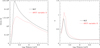Fig. 11.

Velocity and temperature gradients in SFCT stellar models with the new boundary conditions discussed in this paper. Left panel: velocity profile in the outer layers. Right panel: Temperature gradient of the medium ∇ in the same region. Both are displayed as a function of log P in the atmosphere of the 1.0 M_⊙ at the Sun’s position (log L/L_⊙ = 0 and log T_eff = 3.762). The new boundary conditions are applied for log P ≤ 6.0. In both panels we show the results for the MLT and SFCT as indicated.

The key point to note of this tortuous reasoning on the boundary conditions is the confinement of the maximum extension (size) attainable by a convective element over the timescale allowed for its growing is layer by layer compared to and limited by the distance of the layer under consideration to the surface of the star. By doing so, the size of the element grows with depth in agreement with numerical simulations of convection.

The evolutionary track of the 1.0 M_⊙ with the chemical composition [X = 0.703, Y = 0.280, Z = 0.017] calculated from the main sequence to advanced stages along the RGB and in which the outermost layers of the external convective zone are calculated with the new boundary conditions is shown in Fig. 12 and compared with the evolutionary track for the same mass and chemical composition but calculated with the old simple boundary conditions. The reference case of the classical calibrated MLT is shown for comparison. On the HRD, old and new boundary conditions yield the same result. The key difference among new and old boundary condition resides in the better profiles of velocity and temperature gradients across the convective region.

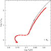Fig. 12.

Evolutionary tracks of 1.0 M_⊙ star with chemical composition [X = 0.703, Y = 0.280, Z = 0.017] calculated with the SFCT and the new boundary conditions (red dots) and the old boundary conditions (blue squares) and the MLT with Λ_m = 1.68 (black crosses). The SFCT models with the old and new boundary conditions fully overlap each other. No significant difference is found among the three cases from the main sequence up to the bottom of the RGB. As already noticed by Pasetto et al. (2016), the RGB with the SFCT is more inclined compared to the correspondent one obtained from the MLT (see the text for more details on this issue).

There is a final consideration worth being made here. In the new boundary conditions for regions A and B, the growth of the element size (ξ_e) is limited by the imposition that it cannot exceed the length corresponding to the distance of the layer under consideration to the surface of the star (in the deeper C region, this is not necessary). This may be taken as some form of closure that a fully self-consistent model should not require. A more realistic treatment of the convective-radiative boundary requires introducing additional constraints which the solution of the SFCT model have to fulfill. The issue is left to future investigation.

To conclude, the group of Eqs. (53)–(55) are the new and better boundary conditions for the convection in the atmosphere of a star according to SFCT. With the aid of these, evolutionary models for the 1.0 M_⊙ with the chemical composition [X = 0.703, Y = 0.280, Z = 0.017] are calculated from the main sequence to advanced stages along the RGB. The evolutionary track is shown in Fig. 12 and compared with the one with the same mass and chemical composition, except for the old boundary conditions and the one obtained from the MLT. First of all, the old and new boundary conditions yield the same results (at least for the stellar models we calculated). In fact, the two tracks fully overlap for all computed models. However, the new boundary conditions are to be preferred because of their better internal consistency. Second, both cases are in close agreement with the corresponding models calculated with the MLT. However, as already noticed by Pasetto et al. (2016), in this case the red giant branches of the SFCT models are again redder compared with the one obtained from the MLT.

5.3. ML equivalent parameter Λ

We can derive the analog of the mixing length parameter to be associated to the SFCT. In other words, the results of the SFCT can be read off in terms of the MLT formalism.

Let us start from the following linear proportionality relationship:

$\begin{matrix} v^{'} : v_{asy} = v_{a} : v_{s}, \end{matrix}$ $\begin{aligned} { v}^\prime : { v}_{\rm asy}={ v}_{\rm a} : { v}_{\rm s} , \end{aligned}$ (56)

where v_asy is the convective velocity when the asymptotic regime is reached, v′ the velocity associated with the accelerations used in relations (51) and (52) above, and v_a the limit velocity given by the product of the maximum acceleration times the asymptotic time. It is obvious that if v_a > v_s, then v_a = v_s, because v_s is the maximum possible velocity for v′=v_asy. This equation holds thanks to the nearly constant nature of the first derivative of the velocity with respect to time (∂v/∂t ≃ const), in the SFCT (see Fig. 7 in Pasetto et al. 2014). If we compare the expression of the velocity in the MLT with that obtained from the linear approximation of the expression in the SFCT, we obtain the following equation:

$\begin{matrix} \frac{v_{MLT}^{2}}{v_{SFCT}^{2}} = \frac{{(\nabla - \nabla_{e})}_{MLT}}{{(\nabla - \nabla_{e})}_{SFCT}} \frac{Λ_{ML}^{2} h_{p}^{2}}{Δ R ξ_{e}} \frac{3}{16}, \end{matrix}$ $\begin{aligned} \frac{{ v}_{\rm MLT}^2}{{ v}_{\rm SFCT}^2}=\frac{(\nabla -\nabla _{\rm e})_{\rm MLT}}{(\nabla -\nabla _{\rm e})_{\rm SFCT}} \frac{\Lambda _{\rm ML}^2 h_{\rm p}^2}{\Delta R \xi _{\rm e}}\frac{3}{16} , \end{aligned}$ (57)

where the velocity of the ML theory has been replaced by its expression as a function of the ML parameter Λ_ML (in this subsection, Λ_m is simply indicated by Λ_ML). Thanks to this, the mixing length parameter Λ_ML associated with the MLT can be expressed as a function of velocity and other quantities of the SFCT:

$\begin{matrix} Λ_{ML} = Λ_{o} \frac{v_{MLT}}{v_{SFCT}}, \end{matrix}$ $\begin{aligned} \Lambda _{\rm ML}=\Lambda _o \frac{{ v}_{\rm MLT}}{{ v}_{\rm SFCT}}, \end{aligned}$ (58)

with Λ_o given by

$\begin{matrix} Λ_{o} = {[\frac{{(\nabla - \nabla_{e})}_{SFCT}}{{(\nabla - \nabla_{e})}_{MLT}} \frac{Δ R ξ_{e}}{h_{p}^{2}} \frac{16}{3}]}^{0.5} . \end{matrix}$ $\begin{aligned} \Lambda _o = \left[\frac{(\nabla -\nabla _{\rm e})_{\rm SFCT}}{(\nabla -\nabla _{\rm e})_{\rm MLT}} \frac{\Delta R \xi _{\rm e}}{h_{\rm p}^2}\frac{16}{3}\right]^{0.5} . \end{aligned}$ (59)

We introduce the suffix ML in the expression for Λ to remind the reader that this quantity plays a role only in the context of the MLT. In the Tables 1 and 2, we show the values of Π, Π′, ξ_e/D, Λ₀, and Λ_ML as a function of position (log P) in the outer convective zone both for the Sun and a model along the RGB. Looking at the layer in which ξ_e/D ≃ 1.0 and Π is minimum, we obtain the value Λ_ML = 1.716 for the Sun and Λ_ML = 1.838 for the model on the RGB. The result for the Sun is fully consistent with the initial assumption for Λ_ML in the evolutionary models (i.e., 1.68). The result for the RGB is more intriguing. The slope of the new RGB is more inclined with respect to the RGB calculated with the MLT. To obtain formal coincidence, one would require an RGB with a lower value of Λ_ML in the MLT, that is, the ML parameter should change with the evolutionary phase. The value for Λ_ML predicted by our analysis is both fully consistent with a constant value along the evolutionary sequence and a slightly varying value. The analysis is too crude to allow more stringent conclusions. We invite the reader to consult Magic et al. (2015) for similar results concerning possible variations of Λ_ML with the evolutionary stage.

Table 1.

Most external layers of the atmosphere of the model with chemical composition [X = 0.703, Y = 0.280, Z = 0.017], log L/L_⊙ = 0. log T_eff = 3.762, age = 4.6 Gyr best reproducing the position of the Sun in the HR diagram.

Table 2.

Same as in Table 1, but for the model along the RGB with log L/L_⊙ = 1.489, log T_eff = 3.638, and age of ≃11 Gyr.

6. Three important checks of the SFCT

6.1. Numerical validation of the SFCT

After arguing the meaning of the mixing-length parameter and highlighting the essence of the SFCT, we present a simple numerical test of the physical reasons why the SFCT can remove the mixing-length problem and why the uniqueness theorem presented in Pasetto et al. (2014) holds well. As a result of this test, not only can we better understand the theory of Pasetto et al. (2014), but we can also derive a numerical counterpart of the analytical derivation of the set of equations presented by Pasetto et al. (2016). The test does not require complicated stellar structure codes; it can be done with a pocket calculator.

We chose the same layer of the standard solar model already examined by Pasetto et al. (2014). The layer is close to the surface, where the energy transport is far from being super-adiabatic. Hence, the effect of the SFCT (or MLT) is more substantial and relevant. We use the same input values for our calculation in MLT and SFCT and adopt SI units. The input values are r = 6.92002 × 10⁸ m, T = 48503.4 K, ∇_ad = 0.28310, ∇_rad = 295186.6, p^∞ = 2.05058 N m⁻², g = 277.517 m s⁻², ρ = 0.345519 kg m⁻³, and $c_{p}^{\infty} = 102986.2 J {kg}^{-1} K$ $c_{\rm p}^\infty = 102986.2 \,{\rm J \, kg^{ - 1}\, K}$ for stellar radius, temperature, adiabatic gradient, radiative gradient, pressure of the stellar layer far away from the convective element, gravity in the same layer, average density, and specific heat at constant pressure far away from the convective element. In addition to these values, three universal constants must be specified: the gravity constant G = 6.67428 × 10⁻¹¹ m³ K g⁻¹ s⁻², the gas radiation density constant a = 7.56464 × 10⁻¹⁶ J K⁻⁴ m⁻³, and the speed of light c = 2.99792 × 10⁸ m s⁻¹.

We first obtain a solution for the radiative-convective-conductive transport of energy with the MLT. For this we use Eqs. (B1), (B2), and (B3) of Pasetto et al. (2016). To proceed we need the mixing length of l_m = Λ_mh_p with Λ_m = 1.68 and $h_{p} = \frac{p^{\infty}}{ρ g}$ ${h_{\mathrm{p}}} = \frac{{{p^\infty }}}{{\rho g}}$ (e.g., Bertelli et al. 2008). With these entries, the quantities V and W of Eq. (B2) are

$\begin{matrix} V = \frac{3 a c T^{3}}{c_{p}^{\infty} ρ^{2} κ l_{m}^{2}} \sqrt{\frac{8 h_{p}}{g δ}} = 1.95043 \times 10^{- 11} \end{matrix}$ $\begin{aligned} V = \frac{{3ac{T^3}}}{{c_{\rm p}^\infty {\rho ^2}\kappa l_m^2}}\sqrt{\frac{{8{h_{\rm p}}}}{{g\delta }}} = 1.95043 \times {10^{ - 11}} \end{aligned}$

and

$\begin{matrix} W = \nabla_{rad} - \nabla_{ad} = 295186.3 . \end{matrix}$ $\begin{aligned} W = {\nabla _{{\text{ rad}}}} - {\nabla _{{\text{ ad}}}} = 295186.3. \end{aligned}$

The expression for Eq. (B3) becomes

$\begin{matrix} {(x - 1.950 \times 10^{- 11})}^{3} + (1.733 \times 10^{- 11}) (x^{3} - 2.951 \times 10^{5}) = 0, \end{matrix}$ $\begin{aligned} {\left( {x - 1.950 \times {{10}^{ - 11}}} \right)^3} + \left( {1.733 \times {{10}^{ - 11}}} \right)\left( {{x^3} - 2.951 \times {{10}^5}} \right) = 0, \end{aligned}$

with

$\begin{matrix} x^{2} = \nabla - \nabla_{ad} + V^{2} . \end{matrix}$ $\begin{aligned} {x^2} = \nabla - {\nabla _{{\text{ ad}}}} + {V^2}. \end{aligned}$

This is the classic cubic equation of the MLT. Using Eqs. (B4), (B5), and (B6) of Pasetto et al. (2016), one can derive the analytical solution. Alternatively, a numerical solution can be used (e.g., Press et al. 1992) to obtain x = 0.01723 for our layer. Finally, with this value for x, we derive ∇ = 0.28340.

We then repeat the same calculations, but use the SFCT for which no assumption has to be made for the mixing length parameter Λ_m, simply because this parameter is missing in the equations of this theory. We start from Eq. (12) of Pasetto et al. (2016), and we proceed backward to obtain ∇. All the details of the procedure can be found in Pasetto et al. (2014) and Pasetto et al. (2016). We use the same input values and take a sufficiently long time interval to ensure that the asymptotic regime is reached for all relevant quantities (the velocity in particular). It is worth recalling here that the asymptotic regime is a consequence of the uniqueness theorem (see Pasetto et al. 2014, Sect. 6.2). From a numerical point of view, we consider the asymptotic regime to be reached when the velocity of convective elements does no longer change more than a few percent (the corresponding integration time is about t = 10⁶s). This is a rather long timescale, close to the turnover time for the entire convective region, and much longer than the dynamical timescale in the same layers. On one hand, this implies that the timescales required by the SFCT are in the range derived from observations and 3D simulations. On the other hand, on those timescales significant evolution of the flow pattern will have occurred. This may be a point of uncertainty of the SFCT.

The basic quintic equation of the SFCT is⁴

$\begin{matrix} \sum_{i = 0}^{5} c_{i} {\bar{v}}^{i} = 0, \end{matrix}$ $\begin{aligned} \sum \limits _{i = 0}^5 {{c_i}{\bar{ v}^i} = 0}, \end{aligned}$ (60)

whose coefficients and associated numerical values are as follows:

$\begin{matrix} c_{5} = 1, \\ c_{4} = \frac{h_{p}}{2 δ \nabla_{ad} t} = 37.7687, \\ c_{3} = \frac{8 α (\nabla_{ad} + 2 \nabla_{rad})}{9 \nabla_{ad} t} = 3.75137, \\ c_{2} = \frac{4 α v^{2} (2 δ g_{4} t (\nabla_{ad} - \nabla_{rad}) \sqrt{\bar{χ}} + 3 h_{p})}{9 δ \nabla_{ad} τ^{2}} = 3.75 \times 10^{6}, \\ c_{1} = \frac{32 α^{2} \nabla_{rad}}{3 \nabla_{ad} \bar{χ}} = 0.000546, \\ c_{0} = \frac{16 α^{2} h_{p}}{3 δ \nabla_{ad} τ \bar{χ}} = 1.97995 \times 10^{- 8}, \end{matrix}$ $\begin{aligned}&{c_5} = 1, \nonumber \\&{c_4} = \frac{{{h_{\rm p}}}}{{2\delta {\nabla _{{\text{ ad}}}}t}} = 37.7687,\nonumber \\&{c_3} = \frac{{8\alpha ({\nabla _{{\text{ ad}}}} + 2{\nabla _{{\text{ rad}}}})}}{{9{\nabla _{{\text{ ad}}}}t}} = 3.75137, \nonumber \\&{c_2} = \frac{{4\alpha {{ v}^2}\left( {2\delta {g_4}t\left({\nabla _{{\text{ ad}}}} - {\nabla _{{\text{ rad}}}}\right)\sqrt{\bar{\chi }} + 3{h_{\rm p}}} \right)}}{{9\delta {\nabla _{{\text{ ad}}}}{\tau ^2}}} = 3.75 \times 10^6, \nonumber \\&{c_1} = \frac{{32{\alpha ^2}{\nabla _{{\text{ rad}}}}}}{{3{\nabla _{{\text{ ad}}}}\bar{\chi }}} = 0.000546, \nonumber \\&{c_0} = \frac{16 \alpha ^2 h_{\rm p}}{3 \delta \nabla _{\text{ ad}} \tau \bar{\chi }} = 1.97995 \times 10^{-8}, \end{aligned}$ (61)

with

$\begin{matrix} α \equiv \frac{a c T^{3}}{κ ρ^{2} c_{p}} . \end{matrix}$ $\begin{aligned} \alpha \equiv \frac{a c T^3}{\kappa \rho ^2 c_{\rm p}}. \end{aligned}$ (62)

This equation has three real solutions and two complex ones. The only physically acceptable solution is $\bar{v} = 194.607 m s^{- 1}$ $\bar {v} = 194.607 \,\mathrm{m \, s^{ - 1}}$ . After the selection of the root, the determination of ∇ becomes straightforward. Finally, we obtain ∇_SFCT = 0.28310 for the stellar layer under examination, which is virtually indistinguishable from the result of the MLT: ∇_MLT = 0.28340. The “mixing-length problem” is numerically solved; equalities between the left hand side (LHS) and right hand side (RHS) of the system of equations are recovered and verified (within the precision error), and the Sun modeled with MLT and with SFCT is the same, that is, it has the same star pressure–temperature stratification.

An obvious criticism is that the layer we examined is not the best choice, because it is located in the region of quasi adiabatic regime so that any reasonable convection theory would predict the same results. Since the SFCT and the MLT with Λ_m = 1.68 yield the same radius (see the HRDs of Figs. 7 and 12) and internal structure of the layer, the numerical agreement we have found is a natural consequence. Examining more external layers, where the super-adiabatic regime holds, would be more informative. We have already seen that the velocity and temperature gradient profiles in this region derived from the MLT and the SFCT with the new boundary conditions (see Fig. 11) are quite similar, thus implying that a numerical check in this layer would yield similar results. One may question if the equality of the SFCT and MLT radii for the Sun is just a coincidence. We do not think it is, because the SFCT and MLT evolutionary tracks for the mass and chemical composition of the Sun coincide from the zero age main sequence all the way up to the bottom of the RGB.

6.2. Time-dependent Schwarzschild and Ledoux criteria

By extending the detailed study of the above layer in the external convective region of the evolutionary sequence representing the Sun to different evolutionary stages, one may have an idea of the timescale needed for the velocity, temperature gradients ∇_e and ∇, and convective flux φ_cnv to reach their regime values. The results are displayed in Fig. 13, from which we extract a few more essential features of the SFCT.

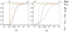Fig. 13.

Evolution of averaged fluxes, gradients, and velocity for a 1 M_⊙ stellar model with log₁₀L/L_⊙ = 0.0, log₁₀T_eff = 3.76 and solar metallicity. Left panel refers to R = 0.7 R_⊙, right panel to R = 0.88 R_⊙. Data are from Pasetto et al. (2019).

The stability criteria of Schwarzschild and Ledoux express the condition for the onset of the convection. More precisely, they predict the boundaries of stability to instability but they cannot say anything about the timescale over which an unstable layer becomes effective in carrying the convective flux, in other words when the convective flux across the unstable region reaches the stationarity regime. This is possible with the SFCT, which predicts a non-null time interval for convection to become effective. For the sake of simplicity, we refer to a stellar layer L as “convective”, if (and only if) both the conditions,

$\begin{matrix} {\begin{matrix} \nabla_{rad} > \nabla > \nabla_{e} > \nabla_{ad} \\ φ_{rad / cnd} < φ_{cnv}, \end{matrix} \end{matrix}$ $\begin{aligned} \left\{ \begin{array}{l} {\nabla _{{\text{ rad}}}} > \nabla > {\nabla _{\rm e}} > {\nabla _{{\text{ ad}}}} \\ {\varphi _{\rm rad/cnd}} < {\varphi _{{\text{ cnv}}}}, \\ \end{array} \right. \end{aligned}$ (63)

are satisfied ∀t. In the conditions above, φ_rad, φ_cnd, and φ_cnv are the radiative, conductive, and convective flux, respectively. Despite all the figures referring to layers where the classic Schwarzschild criterion is satisfied, ∇_rad > ∇ > ∇_e > ∇_ad, the onset of the convection initially presents a still radiative dominated energy transfer; that is, while φ_rad/cnd > φ_cnv, and only after a small amount of time of the order of 100 seconds for a star of solar type (but it can be as large as 10⁶ s for a giant star) does the energy flux become dominated by convection (i.e., both the criteria of Eq. (63) are matched). Moreover, we note how the timescale with which ∇ = ∇(t) and φ_rad/cnd = φ_rad/cnd(t) develop is always the same. This is a natural result because both are proportional to each other, $φ_{rad / cnd} = \frac{4 c}{3} \frac{a T^{4}}{κ h_{p} ρ} \nabla$ ${{\varphi }_{\mathrm{rad/cnd}}}=\frac{4c}{3}\frac{a{{T}^{4}}}{\kappa {{h}_{\mathrm{p}}}\rho }\nabla$ , that is, φ_rad/cnd ∝ ∇ with a constant proportionality factor. Furthermore, because of Eq. (63), we see that φ_rad/cnd < φ_cnv is in agreement with the definition of convectively unstable layers.

Finally, the average velocity of the convective elements is the variable most sensitive to the physics of the star. In our case, Fig. 13 shows the sole positive average velocities $\bar{v} > 0$ $\bar {v} > 0$ . Analogous analysis can be done for the negative velocities $\bar{v} < 0$ $\bar {v} < 0$ with similar results. From similar figures referring to other evolutionary stages of the same star or other stars, the timescale with which the asymptotic mean-stream velocity is reached by the convective elements, before dissolving by RT and KH effects, can be as short as a few hundred seconds as well as long as 10⁶s for stars of large dimensions. Although the predictions about the finite time required for the onset of a fully efficient convective flux in convectively unstable regions is of little practical use because the involved timescales are very short compared to the evolutionary time scale of a star, it was interesting to point them out.

6.3. On the approximation of a subsonic regime in the SFCT

Extending the above numerical investigation, we may check whether the approximation of subsonic regime adopted in the SFCT is physically grounded. This corresponds indeed to a numerical validation of the Lemma 1 in Pasetto et al. (2014), another point strongly criticized by Miller Bertolami et al. (2016) that needs to be clarified. The limitation to subsonic regimes (one of the basic hypotheses of the SFCT) leads to the conditions (see Pasetto et al. 2014, Lemma 1)

$\begin{matrix} {(\frac{\bar{v}}{\dot{R}})}^{2} \frac{1}{2} (\frac{9}{4} {sin}^{2} θ - 1) ≪ A \frac{R}{{\dot{R}}^{2}} (\frac{3}{2} cos θ - cos ϕ) + \frac{\ddot{R} R}{{\dot{R}}^{2}} \end{matrix}$ $\begin{aligned} {\left( {\frac{\bar{ v}}{{{{\dot{R} }}}}} \right)^2}\frac{1}{2}\left( {\frac{9}{4}{{\sin }^2}\theta - 1} \right) \ll A\frac{{{R }}}{{\dot{R} ^2}}\left( {\frac{3}{2}\cos \theta - \cos \phi } \right) + \frac{{{{\ddot{R} }} {R }}}{{\dot{R} ^2}}\end{aligned}$ (64)

or

$\begin{matrix} {(\frac{\bar{v} \dot{R}}{{\dot{R}}^{2}})}^{2} \frac{5}{2} cos θ ≪ A \frac{R}{{\dot{R}}^{2}} (\frac{3}{2} cos θ - cos ϕ) + \frac{\ddot{R} R}{{\dot{R}}^{2}}, \end{matrix}$ $\begin{aligned} {\left( {\frac{{\bar{ v}{{\dot{R} }}}}{{\dot{R} ^2}}} \right)^2}\frac{5}{2}\cos \theta \ll A\frac{{{R }}}{{\dot{R} ^2}}\left( {\frac{3}{2}\cos \theta - \cos \phi } \right) + \frac{{{{\ddot{R} }}{R }}}{{\dot{R} ^2}}, \end{aligned}$ (65)

the validity of which can be tested numerically using an extended set of model atmospheres (external envelopes) of stellar models (Sun included). We start defining three functions from the above Eqs. (64) and (65):

$\begin{matrix} f (t, θ) \equiv {(\frac{\bar{v}}{\dot{R}})}^{2} \frac{1}{2} (\frac{9}{4} {sin}^{2} θ - 1), \\ g (t, θ) \equiv {(\frac{\bar{v} \dot{R}}{{\dot{R}}^{2}})}^{2} \frac{5}{2} cos θ, \\ k (t, θ) \equiv A \frac{R}{{\dot{R}}^{2}} (\frac{3}{2} cos θ - cos ϕ) + \frac{\ddot{R} R}{{\dot{R}}^{2}} . \end{matrix}$ $\begin{aligned}&f\left( {t,\theta } \right) \equiv {\left( {\frac{\bar{ v}}{{{{\dot{R} }}}}} \right)^2}\frac{1}{2} \left( {\frac{9}{4}{{\sin }^2}\theta - 1} \right), \nonumber \\&g\left( {t,\theta } \right) \equiv {\left( {\frac{{\bar{ v}{{\dot{R} }}}}{{\dot{R} ^2}}} \right)^2}\frac{5}{2} \cos \theta , \\&k\left( {t,\theta } \right) \equiv A\frac{{{R }}}{{\dot{R} ^2}}\left( {\frac{3}{2}\cos \theta - \cos \phi } \right) + \frac{{{{\ddot{R} }}{R }}}{{\dot{R} ^2}}. \nonumber \end{aligned}$ (66)

We consider the same layer L already introduced in Sect. 6. Other quantities that may be required to perform the test are either available in Table 1 of Pasetto et al. (2014) or are explicitly calculated; for instance derivatives such as Ṙ and others are given by the tangents to the curve representing the variable in question (see Fig. 13). For the same layer inside the Sun already analyzed in Sect. 6.3 of Pasetto et al. (2014; but after about 10⁶s), we have $\bar{v} = 194.6 km s^{- 1}$ $\bar {v} = 194.6\,\mathrm{km\,s^{ - 1}}$ and $\bar{χ} = 8.3 \times 10^{10}$ $\bar \chi = 8.3 \times {10^{10}}$ . Looking at the point on the surface of the element with θ = 0, we obtain f(10⁶,0) = −6.81 × 10⁻⁷. At the same time and location, we have ${\bar{v}}^{'} = 1.027 \times 10^{- 5} km s^{- 2}$ $\bar{\mathit{v}}^\prime = 1.027 \times {10^{ - 5}}\,\mathrm{km\,s^{ - 2}}$ , ${\bar{χ}}^{'} = 1.666 \times 10^{5}$ $\bar \chi^\prime = 1.666 \times {10^5}$ and ${\bar{χ}}^{″} = 0.156$ $\bar \chi^{\prime\prime} = 0.156$ . It follows that k(10⁶,0) = 0.5. It is evident that the first of the equations necessary to prove the Lemma 1, f(t,θ) ≪ k(t,θ), of Pasetto et al. (2014) has been verified. Now that all the values are available, it is a simple exercise to also prove that the second g(t,θ) ≪ k(t,θ).

This result may change if we perform the same exercise for any point θ or ϕ on the surface of a convective element. This is shown in Fig. 14. As evident, the conditions f(t,θ) ≪ k(t,θ) and g(t,θ) ≪ k(t,θ) are always verified in the temporal regime of interest (as correctly mathematically proved in Lemma 1). This is contrary to what was claimed in Miller Bertolami et al. (2016), where the authors apparently find, for the same solar model and using the same equations, that the conditions expressed by Eqs. (64) and (65) are violated. This is exactly the opposite of what we find here. The reasons for this contrasting result are not clear. The numerical test presented here is a necessary check of internal consistency of the SFCT aimed to confute the claim by Miller Bertolami et al. (2016); no other conclusion can be drawn from it.

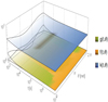Fig. 14.

Numerical validation of Lemma 1 in Pasetto et al. (2014). The functions g,f, and k are defined in the text and plotted against the values of interest in the Lemma 1, i.e., in the “asymptotic” regime of validity of the uniqueness theorem. Evidently, the blue manifold always remains above the green and yellow ones for all the timescales of interest and for any angular dependence of the equations. This temporal interval covers all the stars calculated by Pasetto et al. (2016). Data are from Pasetto et al. (2019).

7. Limits to the validity of the SFCT

7.1. Timescale of the uniqueness theorem

We wish to comment that the solution of the convective energy transport, i.e., the determination of all physically relevant quantities (velocity, size, etc.) of convective elements, is achieved by the SFCT thanks to the uniqueness theorem (Pasetto et al. 2014, Sect. 6.2), which, however, can only be applied in the framework of a linear-response theory. Consequently, the SFCT inherits the limits of this theorem. The implications of this limitation are better understood with an example. The theorem states that, at the linear order, there is an invariant manifold solution of the system of equations for the energy transfer inside a star. If a solution is invariant, we might be tempted to obtain the invariance regime directly from the quintic Eq. (60) by pushing the temporal limit of the coefficients in Eq. (61) to infinity and thus obtaining the following after simple manipulations:

$\begin{matrix} lim_{τ \to \infty} (lim_{χ \to τ^{2}} (\sum_{i = 0}^{5} c_{i} {\bar{v}}^{i})) = \frac{1}{9} {\bar{v}}^{2} (\frac{8 α g_{4} (\nabla_{ad} - \nabla_{rad})}{\nabla_{ad}} + 9 {\bar{v}}^{3}) = 0 . \end{matrix}$ $\begin{aligned} \mathop {\lim }\limits _{\tau \rightarrow \infty } \left( {\mathop {\lim }\limits _{\chi \rightarrow {\tau ^2}} \left( {\sum \limits _{i = 0}^5 {{c_i}{\bar{ v}^i}} } \right)} \right) = \frac{1}{9}{\bar{ v}^2}\left( {\frac{{8\alpha {g_4}({\nabla _{{\text{ ad}}}} - {\nabla _{{\text{ rad}}}})}}{{{\nabla _{{\text{ ad}}}}}} + 9{\bar{ v}^3}} \right) = 0. \end{aligned}$

Apparently, in this way we reduce the quintic to a cubic (as in the MLT case) whose only real solution for a convective region would be

$\begin{matrix} \bar{v} = \frac{2 \sqrt[3]{α g_{4} (\nabla_{rad} - \nabla_{ad})}}{3^{2 / 3} \sqrt[3]{\nabla_{ad}}} . \end{matrix}$ $\begin{aligned} \bar{ v} = \frac{{2\root 3 \of {{\alpha {g_4}\left( {{\nabla _{{\text{ rad}}}} - {\nabla _{{\text{ ad}}}}} \right)}}}}{{{3^{2/3}}\root 3 \of {{{\nabla _{{\text{ ad}}}}}}}}. \end{aligned}$

This is also confirmed by a numerical investigation of the coefficients in Eq. (61); taking $\sum_{i = 0}^{5} \frac{c_{i} {\bar{v}}^{i}}{{\bar{v}}^{2}} = 0$ $\sum\limits_{i = 0}^5 {\frac{{{c_i}{\bar {v}^i}}}{{{\bar {v}^2}}}} = 0$ and neglecting {c₄,c₅} ≪ {c₁,c₂,c₃}, we can obtain a solution for $\bar{v}$ $\bar {v}$ of the resulting cubic that is completely indistinguishable from the $\bar{v}$ $\bar {v}$ obtained from the quintic.

Unfortunately, despite its apparent simplicity, this way of using the uniqueness theorem is wrong because it is outside its founding hypotheses. As explained in Pasetto et al. (2014), the “limit τ → ∞” is a mathematical idealization for the dimensionless independent variable (τ in our case) to reach the asymptotic behavior of the solution, say for t > t^∞. In the real case of interest, τ cannot exceed a specific limit value, securing that (i) the stellar region under consideration is still convective; (ii) the convective elements are still moving inside the convective regions; and (iii) the star itself does still exist. The real physical limit “τ → ∞” (or “τ → ∂L” in the example of Sect. 4) is set by the state variables p = p(x;t), density ρ = ρ(x;t), and temperature T = T(x;t) with the time t, so the limit of Eq. (62),

$\begin{matrix} lim_{τ \to \infty} α = lim_{τ \to \infty} \frac{a c T^{3}}{κ ρ^{2} c_{p}}, \end{matrix}$ $\begin{aligned} \mathop {\lim }\limits _{\tau \rightarrow \infty } \alpha = \mathop {\lim }\limits _{\tau \rightarrow \infty } \frac{{ac{T^3}}}{{\kappa {\rho ^2}{c_{\rm p}}}}, \end{aligned}$

is coherently accounted for. However, it is simple to prove that in such a case the SFCT flattens the gradients in the state variables to their adiabatic stratifications: $lim_{τ \to \infty} \nabla = lim_{τ \to \infty} \nabla_{e} = \nabla_{ad}$ $\mathop {\lim }\limits_{\tau \to \infty } \nabla = \mathop {\lim }\limits_{\tau \to \infty } {\nabla _{\mathrm{e}}} = {\nabla _{{\text{ ad}}}}$ and the size of the convective element would diverge $lim_{τ \to \infty} χ = \infty$ $\mathop {\lim }\limits_{\tau \to \infty } \chi = \infty$ as expected (indeed, one of the primary effects of convection is homogenizing the stellar gradients).

7.2. The effects of turbulence on stellar convection

One of the present limitations of the SFCT is that even a simple description of turbulence is missing. Turbulence is among the largely uncertain phenomena of physics. It is expected to affect the SFCT both at the onset of convection, e.g., for t < t⁰, and in its stationary regime, say for t ≃ t^∞, as shown in Fig. 13 limited to a typical case.

The fact that the MLT has the same severe limitations does not help at all. Indeed, it has long been recognized that MLT has been repeatedly falsified. (i) It predicts the wrong frequencies of solar p modes (Nordlund et al. 2009; Houdek & Dupret 2015). (ii) Spectral line shapes implied by MLT model atmospheres need corrections to avoid errors in abundance determinations. (iii) Overshooting observed at the solar surface is ignored. (iv) Photometric colors from 1D model atmospheres are mispredicted (Smalley & Kupka 1997). Finally, we have already quoted a number of studies based on 3D hydrodynamical numerical simulations that require accounting for turbulence in stellar convection. Nevertheless, the classical MLT is still a useful model in stellar model calculations that have been used to generate isochrones and synthetic color–magnitude diagrams of globular cluster stars from the main sequence to the RGB and beyond (see Brown et al. 2005, to mention just one). The SFCT follows the MLT in these matters; most likely it cannot improve the situation as far as the above issues are concerned. Several approaches are available in the literature to account for turbulence parametrically, as well as a large body of results from 3D hydrodynamics simulations (see Kupka & Muthsam 2017 for a recent review and exhaustive referencing).

Therefore, in this section instead of arguing in favor of neglecting turbulence in the SFCT, we limit ourselves to evaluating the relevance of energy exchange between the mean convective flow and the turbulence in the regime t ≃ t^∞. The regime $t < t_{}^{0}$ $t < t_{}^{0}$ , introduced in Sect. 4.1 as a limit case for the SFCT in a homogeneous isotropic medium, is not of interest here.

If we assume that the distribution function of the turbulent cascade of the stellar plasma (in S₀) is given by f₀ = f₀(x,v;t), the mean flow is just the first-order moment of this distribution ${\bar{v}}_{0} = \int_{}^{} v_{0} f_{0} (x, v ; t) d^{3} x$ ${{\boldsymbol{\bar{\mathit{v}}}}_{0}}=\int_{}^{}{{{\boldsymbol{v}}_{0}}{{f}_{0}}\left( \boldsymbol{x},\boldsymbol{v};t \right){{d}^{3}}\boldsymbol{x}}$ , while the second-order moment $σ_{0}^{2} = \int_{}^{} {(v_{0} - {\bar{v}}_{0})}^{\otimes 2} f d^{3} x$ $\boldsymbol{\sigma }_{0}^{2}=\int_{}^{}{{{\left( {{\boldsymbol{v}}_{0}}-{{{\boldsymbol{\bar{\mathit{v}}}}}_{0}} \right)}^{\otimes 2}} f{{d}^{3}}\boldsymbol{x}}$ (with *^⊗2 being the ordinary tensor product of order n). Because we are only interested in the case t ≃ t^∞, we simplify the moments as $\int_{}^{} v_{0} f_{0} (x, v ; t ≃ t^{\infty}) d^{3} x = v_{0}^{\infty},$ $\int_{}^{}{{{\boldsymbol{v}}_{0}}{{f}_{0}}\left( \boldsymbol{x},\boldsymbol{v};t \simeq {{t}^{\infty }} \right){{d}^{3}}\boldsymbol{x}}= \boldsymbol{v}_{0}^{\infty },$ and, similarly, for $σ_{0}^{\infty}$ $\boldsymbol{\sigma }_{0}^{\infty }$ (we omit the square present only for historical reasons, while clearly σ can have negative cross terms.) It is simple to prove that the relation between the first and second moments is $σ_{0}^{2} = \bar{v_{0}^{\otimes 2}} - {\bar{v}}_{0} {\bar{v}}_{0}$ $\boldsymbol{\sigma }_{0}^{2}=\overline{\boldsymbol{v}_{0}^{\otimes 2}}- {{\boldsymbol{\bar{\mathit{v}}}}_{0}}{{\boldsymbol{\bar{\mathit{v}}}}_{0}}$ . If we take the time average of the Navier-Stokes equation, i.e., Eq. (30), we obtain

$\begin{matrix} 〈 v_{0}^{\infty}, \nabla_{x} 〉 v_{0}^{\infty} + \bar{〈 v_{0} - v_{0}^{\infty}, \nabla_{x} 〉 (v_{0} - v_{0}^{\infty})} = \nabla_{x} \frac{p^{\infty}}{ρ^{\infty}} . \end{matrix}$ $\begin{aligned} \left\langle \boldsymbol{v}_{0}^{\infty },{{\nabla }_{\boldsymbol{x}}} \right\rangle \boldsymbol{v}_{0}^{\infty }+\overline{\left\langle {{\boldsymbol{v}}_{0}}-\boldsymbol{v}_{0}^{\infty },{{\nabla }_{\boldsymbol{x}}} \right\rangle \left( {{\boldsymbol{v}}_{0}}-\boldsymbol{v}_{0}^{\infty } \right)}={{\nabla }_{\boldsymbol{x}}}\frac{{{p}^{\infty }}}{{{\rho }^{\infty }}}. \end{aligned}$ (67)

Moreover, noticing that the contribution from $〈 〈 v_{0}^{\infty}, \nabla_{x} 〉, v_{0} - v_{0}^{\infty} 〉$ $\left\langle \left\langle \boldsymbol{v}_{0}^{\infty },{{\nabla }_{\boldsymbol{x}}} \right\rangle ,{{\boldsymbol{v}}_{0}}-\boldsymbol{v}_{0}^{\infty } \right\rangle$ and $〈 v_{0} - v_{0}^{\infty}, \nabla_{x} 〉 v_{0}^{\infty}$ $\left\langle {{\boldsymbol{v}}_{0}}-\boldsymbol{v}_{0}^{\infty }, {{\nabla }_{\boldsymbol{x}}} \right\rangle \boldsymbol{v}_{0}^{\infty }$ cancels out when the time average is performed, we arrive at the Reynolds-averaged Navier-Stokes relationship that is suited to our purpose:

$\begin{matrix} 〈 v_{0}^{\infty}, \nabla_{x} 〉 v_{0}^{\infty} & = - \nabla_{x} \frac{p^{\infty}}{ρ^{\infty}} + 〈 \nabla_{x}, - \bar{(v_{0} - v_{0}^{\infty}) (v_{0} - v_{0}^{\infty})} 〉 \\ = - \nabla_{x} \frac{p^{\infty}}{ρ^{\infty}} - 〈 \nabla_{x}, σ_{0} 〉 . \end{matrix}$ $\begin{aligned} \left\langle {{\boldsymbol{v}}_0^\infty ,{\nabla _{\boldsymbol{x}}}} \right\rangle {\boldsymbol{v}}_0^\infty&= - {\nabla _{\boldsymbol{x}}} \frac{{{p^\infty }}}{{{\rho ^\infty }}} + \left\langle {{\nabla _{\boldsymbol{x}}}, - \overline{\left( {{{\boldsymbol{v}}_0} - {\boldsymbol{v}}_0^\infty } \right)\left( {{{\boldsymbol{v}}_0} - {\boldsymbol{v}}_0^\infty } \right)} } \right\rangle \nonumber \\&= - {\nabla _{\boldsymbol{x}}}\frac{{{p^\infty }}}{{{\rho ^\infty }}} - \left\langle {{\nabla _{\boldsymbol{x}}},{{\boldsymbol{\sigma }}_0}} \right\rangle . \end{aligned}$ (68)

While within any small layer L, p^∞ = const. and ρ^∞ = const., pressure and density retain their spatial dependence within the whole convective zone of volume V that is supposed to be composed of many layers. At different L and within V, we note that p^∞ = p^∞(x) and ρ = ρ^∞(x). Because of the results shown in Fig. 13, the temporal dependence can be safely omitted as the structure of the star remains unchanged over the time interval Δt ≃ t^∞ of interest here. Equation (68) couples the mean flow, v^∞, to the dispersion velocity, $σ_{0}^{\infty}$ $\boldsymbol{\sigma }_{0}^{\infty }$ , that is, to the turbulent motion of the stellar plasma. The components of τ ≡ ρσ₀ are indeed traditionally called the Reynolds stresses and have been the subject of extensive studies in relation to the closure problem (e.g., Pope 2000; Launder & Sandham 2002).

For t ≃ t^∞, the ith component of the force acting on a surface element due to $σ_{0}^{\infty}$ $\boldsymbol{\sigma }_{0}^{\infty }$ is quickly written as $ρ^{\infty} σ_{0}^{\infty} d^{2} S$ ${{\rho }^{\infty }}\boldsymbol{\sigma }_{0}^{\infty } {{d}^{2}}S$ , for example, so that for t ≃ t^∞ the rate of work Ẇ^∞ due to turbulent motions is proportional to $ρ^{\infty} 〈 v_{0}^{\infty}, σ_{0}^{\infty} d^{2} S 〉$ ${{\rho }^{\infty }}\left\langle \boldsymbol{v}_{0}^{\infty },\boldsymbol{\sigma }_{0}^{\infty } {{d}^{2}}S \right\rangle$ for the whole convective shell of the volume V bounded by the surface S. In brief, we can write

$\begin{matrix} \frac{d}{d t} W^{\infty} = \oint_{S} 〈 v_{0}^{\infty}, ρ^{\infty} σ_{0}^{\infty} d^{2} S 〉 = \int_{V} ρ^{\infty} 〈 \nabla_{x}, v_{0}^{\infty} σ_{0}^{\infty} 〉 d^{3} V, \end{matrix}$ $\begin{aligned} \frac{\mathrm{d}}{\mathrm{d}t}{{W}^{\infty }}=\oint \limits _{S}{\left\langle \boldsymbol{v}_{0}^{\infty },{{\rho }^{\infty }} \boldsymbol{\sigma }_{0}^{\infty }{\mathrm{d}^{2}}S \right\rangle }=\int \limits _{V}{{{\rho }^{\infty }}\left\langle {{\nabla }_{\boldsymbol{x}}},\boldsymbol{v}_{0}^{\infty }\boldsymbol{\sigma }_{0}^{\infty } \right\rangle {\mathrm{d}^{3}}V}, \end{aligned}$ (69)

where on the last equality we used the Gauss theorem. Hence, for a unit volume, we obtain that

$\begin{matrix} \frac{d}{d^{3} V} \frac{d}{d t} W^{\infty} & = 〈 \nabla_{x}, v_{0}^{\infty} σ_{0}^{\infty} 〉 \\ = ρ^{\infty} 〈 \nabla_{x}, σ_{0}^{\infty} 〉 v_{0}^{\infty} + ρ^{\infty} σ_{0}^{\infty} 〈 \nabla_{x}, v_{0}^{\infty} 〉 . \end{matrix}$ $\begin{aligned} \frac{\mathrm{d}}{{{\mathrm{d}^3}V}}\frac{\mathrm{d}}{{\mathrm{d}t}}{W^{\infty } }&= \left\langle {{\nabla _{\boldsymbol{x}}}, {\boldsymbol{v}}_0^\infty {\boldsymbol{\sigma }}_0^\infty } \right\rangle \nonumber \\&= {\rho ^\infty }\left\langle {{\nabla _{\boldsymbol{x}}},{\boldsymbol{\sigma }}_0^\infty } \right\rangle {\boldsymbol{v}}_0^\infty + {\rho ^\infty }{\boldsymbol{\sigma }}_0^\infty \left\langle {{\nabla _{\boldsymbol{x}}},{\boldsymbol{v}}_0^\infty } \right\rangle . \end{aligned}$ (70)

This leads us to interpret the term $ρ^{\infty} 〈 \nabla_{x}, σ_{0}^{\infty} 〉$ ${{\rho }^{\infty }}\left\langle {{\nabla }_{\boldsymbol{x}}},\boldsymbol{\sigma }_{0}^{\infty} \right\rangle$ also as a force. Because we defined $σ_{0}^{\infty}$ $\boldsymbol{\sigma }_{0}^{\infty }$ adopting the time average procedure on the (unknown) distribution function, this term cannot create or destroy mechanical energy. It can indeed only represent the rate of change of kinetic energy per unit volume. For the sake of simplicity, we exclude over- or under-shooting of the convective elements so that we can safely assume null the convective flux at the boundary of the convective zone V. Therefore, the divergence $〈 \nabla_{x}, v_{0}^{\infty} σ_{0}^{\infty} 〉$ $\left\langle {{\nabla }_{\boldsymbol{x}}},\boldsymbol{v}_{0}^{\infty }\boldsymbol{\sigma }_{0}^{\infty } \right\rangle$ statistically cancels out, and Eq. (70) balances the LHS with the RHS as follows:

$\begin{matrix} \int_{}^{} - ρ^{\infty} 〈 \nabla_{x}, σ_{0}^{\infty} 〉 v_{0}^{\infty} d V = \int_{}^{} σ_{0}^{\infty} ρ^{\infty} 〈 \nabla_{x}, v_{0}^{\infty} 〉 d V . \end{matrix}$ $\begin{aligned} \int _{}^{}{-{{\rho }^{\infty }}\left\langle {{\nabla }_{\boldsymbol{x}}},\boldsymbol{\sigma }_{0}^{\infty } \right\rangle \boldsymbol{v}_{0}^{\infty }\mathrm{d}V}=\int _{}^{}{\boldsymbol{\sigma }_{0}^{\infty }{{\rho }^{\infty }}\left\langle {{\nabla }_{\boldsymbol{x}}},\boldsymbol{v}_{0}^{\infty } \right\rangle \mathrm{d}V}. \end{aligned}$ (71)

Consequently, if $ρ^{\infty} 〈 \nabla_{x}, σ_{0}^{\infty} 〉$ ${{\rho }^{\infty }}\left\langle {{\nabla }_{\boldsymbol{x}}},\boldsymbol{\sigma }_{0}^{\infty } \right\rangle$ is the force due to $σ_{0}^{\infty}$ $\boldsymbol{\sigma }_{0}^{\infty }$ (per unit volume) acting on the mean flow, then $ρ^{\infty} 〈 \nabla_{x}, σ_{0}^{\infty} 〉 v_{0}^{\infty}$ ${{\rho }^{\infty }} \left\langle {{\nabla }_{\boldsymbol{x}}},\boldsymbol{\sigma }_{0}^{\infty } \right\rangle \boldsymbol{v}_{0}^{\infty }$ is the rate of work of this force, and $- ρ^{\infty} 〈 \nabla_{x}, σ_{0}^{\infty} 〉 v_{0}^{\infty}$ $-{{\rho }^{\infty }}\left\langle {{\nabla }_{\boldsymbol{x}}},\boldsymbol{\sigma }_{0}^{\infty } \right\rangle \boldsymbol{v}_{0}^{\infty }$ is the kinetic energy loss rate from the mean flow as a result of the turbulence that must equal precisely the rate of gain of kinetic energy by turbulence. In light of these considerations, it is evident that $σ_{0}^{\infty}$ $\boldsymbol{\sigma }_{0}^{\infty }$ gives rise to a net force acting on the mean flow whose working rate is negative, meaning that the mean flow supplies energy to the turbulence, and energy is transferred from the mean flow to the turbulence.

In conclusion, we prove that the mean flow is overestimated by the SFCT, which, at the present stage, provides only an upper limit to the convective flux. It is beyond the goal of the present paper to upgrade the SFCT to account for the turbulence cascade.

8. Remarks on the criticisms of the SFC theory

Miller Bertolami et al. (2016) criticized the method of Pasetto et al. (2014, 2016) to derive the SFCT as a suitable tool for implementation in stellar evolution models. The criticism concerned many points, among which we focus on the most relevant. (i) The naiveness and crudeness of our treatment of convection that, as in the MLT, is viewed as made of convective elements distinct from the surrounding medium and for simplicity of spherical shape. The elements are supposed to start expanding from infinitesimal dimensions to a large size (always keeping the spherical shape) by the action of small local temperature fluctuations of the medium itself inducing density variations. Because of the expansion, the elements feel the buoyancy force, rise radiating energy from their surface, and eventually dissolve into the medium, thus securing the net transfer of energy from one layer to another. The dynamics of the convective bubbles are followed in detail. Thanks to this, the usual assumption about the mean free path of convective elements and size, in turn, that is expressed by Λ_mh_p was no longer necessary. Because of this Pasetto et al. (2014) claimed that their new theory is scale-free. (ii) The stellar medium is considered as an ideal, inviscid, and irrotational fluid. These assumptions are in commom with the MLT. To these we have also added the operational hypothesis of incompressibility on a suitable local scale to make the use of the concept of potential flow possible. Finally, the effect of turbulence is left aside. Arguments have been provided to justify the latter hypothesis at least at a first-order approximation. The major novelty is that the motion of the convective elements has been derived under the assumption that convective elements are not in pressure equilibrium with their surrounding medium and that the velocity is derivable from the gradient of a suitable potential. Pressure equilibrium is, however, secured on stellar layer scales so that the hydrostatic equilibrium is achieved layer by layer. Finally, the effect of the boundary layer on the dynamics of the convective elements was neglected. (iii) The claim that the SCFT is time-dependent and nonlocal in space due to the fact that the equations governing the physical properties of convective element need to be integrated in time and followed in space to obtain the asymptotic regime for the dynamical behavior has been confuted. (iv) The general physical assumptions concerning the motion of the convective elements throughout the surrounding medium are the following: (a) expanding spheres moving within a fluid of locally constant density; and (b) departure from local pressure equilibrium; that is, the stellar plasma is not in hydrostatic equilibrium on the surface of the expanding or contracting spherical element, while the latter is moving upward or inward. It is worth commenting here that an element rises and or sinks because it expands or contracts due to internal temperature variations with respect to the surrounding medium. For instance, in the case of expansion, it acts as a piston on the medium. The opposite is when it contracts under the compression of the medium. As shown by Pasetto et al. (2016), hydrostatic equilibrium between an element and medium can only be restored “far away” from the element surface and only after some time has elapsed. Since the sound speed is finite, hydrostatic equilibrium cannot be immediately restored. Indeed, a convective element cannot exist at all if it is assumed to always be in perfect mechanical equilibrium with the environment. Based on these arguments, Pasetto et al. (2016) argued that it is reasonable to assume that condition (12) could be applied. Miller Bertolami et al. (2016) rejected this reasoning and imposed immediate hydrostatic equilibrium, thus deriving

$\begin{matrix} \frac{| v |}{| {\dot{ξ}}_{e} |} = \frac{3 h_{p} Γ_{1}}{ξ_{e}}, \end{matrix}$ $\begin{aligned} \frac{\left| \boldsymbol{v}\right|}{ \left| {{\boldsymbol{\dot{\xi }_{\rm e} }}} \right|} = \frac{3h_{\rm p} \Gamma _1}{\xi _{\rm e}} , \end{aligned}$ (72)

where Γ₁ is the usual generalized adiabatic exponent. The conclusion is that $v / {\dot{ξ}}_{e} ≪ 1$ $\mathit{v}/\dot\xi_{\mathrm{e}} \ll 1$ is not allowed, thus ruling out the linearization parameter adopted by Pasetto et al. (2014). (v) As a consequence of the above strong criticism, the approximation made of Eq. (11), that is, the translation of the Bernoulli equation containing the total velocity potential (vertical motion and expansion or contraction) to the accelerated reference frame S₁ and spherical symmetry would immediately fail. In brief, while Eq. (11) is of general validity, introducing condition (12) here, Eq. (11) becomes Eq. (13). Since condition (12) is rejected, Eq. (13) is no longer valid. However, for the arguments brought to support condition (12), we still make use of this condition. In any case, below we provide the equivalent of Eq. (13) when the condition is no longer applied to the general Eq. (11) and strict instantaneous hydrostatic equilibrium is imposed (Eq. (72)) showing that the classical MLT is recovered. (vi) Miller Bertolami et al. (2016) also criticized the expression of the acceleration presented by Pasetto et al. (2014, their Eq. (26)), which they replace by

$\begin{matrix} \dot{v_{b}} = g \frac{m_{b} - M}{m_{b} + M / 2} - \frac{10}{3} \frac{π R^{2} ρ v_{b} \dot{R}}{m_{b} + M / 2}, \end{matrix}$ $\begin{aligned} \dot{\boldsymbol{{ v}_{\rm b}}} = {\boldsymbol{g}} \frac{m_{\rm b} -M }{m_{\rm b} + M/2} - \frac{10}{3} \frac{\pi R^2 \rho { v}_{\rm b} \dot{R}}{m_{\rm b} +M/2} , \end{aligned}$ (73)

where, owing to the differences between our and their notations, the following correspondences must be taken into account: m_e ≡ m_b, ξ_e ≡ R, $\dot{x i_{e}} \equiv v_{b}$ $\dot{\boldsymbol{xi_{\mathrm{e}}}} \equiv \boldsymbol{\mathit{v}_{\mathrm{b}}}$ . Furthermore, M and m_e are the masses of the displaced fluid and convective element, respectively. The first expression given by Pasetto et al. (2014) contained three mistakes, namely the coefficient 10/3 instead of 2, the factor (m_e + M/2) missing at the denominator of the second term, and finally the sign of the first term. However, Pasetto et al. (2016) pointed out the mistakes and provided the right expression (see also Eq. (18) here). In any case, Miller Bertolami et al. (2016) derived what they claimed to be the correct formulation for the acceleration (see their Eq. (43)), which happens to be identical to that obtained by Pasetto et al. (2016). In any case, Pasetto et al. (2014), and Pasetto et al. (2016) simplified the expression for the acceleration dropping the second term, on the notion that, thanks to condition (12), this term rapidly becomes negligible with respect to the first one (see Eq. (19)). Below, following the arguments given by Miller Bertolami et al. (2016), we do not apply the simplification and make use of the complete expression for the acceleration. (vii) Finally, we would like to say that Miller Bertolami et al. (2016) would also have to reject the MLT, because it is essentially based on the same hypotheses.

9. MLT from SFCT for free

One may question if the MLT is a particular case of the SFCT. To answer the question, the easiest thing to do is to introduce, by hand, the condition for the pressure balance at the surface of a convective element and the surrounding medium, i.e., the key hypothesis of the MLT. We start from the equation linking the expansion or contraction of a convective element already presented in Sect. 2, that is, Eq. (11). This equation is of general validity as it stems from the Bernoulli equation and the assumption made for the velocity potential (no additional approximation is made). Since in the models a convective element moves only radially we can pose θ = 0 and ϕ = 0 without losing in generality so that it becomes

$\begin{matrix} \frac{v^{2}}{2} + \frac{3}{2} \dot{ξ_{e}} v + \frac{A}{2} ξ + \ddot{ξ_{e}} ξ_{e} + \frac{3}{2} {\dot{ξ_{e}}}^{2} = 0 . \end{matrix}$ $\begin{aligned} \frac{{ v}^2}{2}+\frac{3}{2}\dot{\xi _{\rm e}} { v} +\frac{A}{2}\xi +\ddot{\xi _{\rm e}}{\xi _{\rm e}}+\frac{3}{2}\dot{\xi _{\rm e}}^2=0 . \end{aligned}$ (74)

This equation links acceleration A, radial (vertical) velocity v, and expansion or contraction rates $\dot{ξ_{e}}$ $\dot{\xi_{\mathrm{e}}}$ and $\ddot{ξ_{e}}$ $\ddot{\xi_{\mathrm{e}}}$ of a convective element. Pasetto et al. (2014, 2016) supposed that $| v | ≪ | {\dot{ξ}}_{e} |$ ${\left| {\mathit{v}}\right|} \ll \left| {\dot \xi_{\mathrm{e}} }\right|$ so that the first two terms could be neglected. We do not make the same assumption and retain all the terms of this equation.

We now introduce the condition for the strict hydrostatic equilibrium according to Miller Bertolami et al. (2016), that is, $v = \frac{\dot{ξ_{e}}}{ξ_{e}} 3 h_{p} Γ_{1}$ $\mathit{v}=\frac {\dot{\xi_{\mathrm{e}}}} {\xi_{\mathrm{e}}} 3h_{\mathrm{p}}\Gamma_1$ to obtain

$\begin{matrix} \ddot{ξ_{e}} ξ_{e} + \frac{3}{2} {\dot{ξ_{e}}}^{2} [1 + \frac{3 h_{p} Γ_{1}}{ξ_{e}} + \frac{3 h_{p}^{2} Γ_{1}^{2}}{ξ_{e}^{2}}] + \frac{A}{2} ξ_{e} = 0 . \end{matrix}$ $\begin{aligned} \ddot{\xi _{\rm e}}\xi _{\rm e}+\frac{3}{2}\dot{\xi _{\rm e}}^2 \left[1+\frac{3h_{\rm p}\Gamma _1}{\xi _{\rm e}}+\frac{3h_{\rm p}^2 \Gamma _1^2}{\xi _{\rm e}^2} \right]+\frac{A}{2}\xi _{\rm e}=0 . \end{aligned}$ (75)

Thereafter, we drop the subscript “e” because it is superfluous.

It is worth noting that the equation is a function of the layer under consideration via h_p. Comparing with the corresponding equation of Pasetto et al. (2014) or Eq. (13), there are two more terms in the square bracket that originate from terms in Eq. (74) with the velocity v.

At this stage, we consider the three equations defining the radiative flux, the convective flux, and the total flux, φ_rad, φ_cnv, and φ_rad + φ_cnv, respectively, together with the one for the ratio of temperature gradients, $\frac{\nabla_{e} - \nabla_{ad}}{\nabla - \nabla_{e}}$ $\frac{\nabla_{\mathrm{e}}-\nabla_{\mathrm{ad}}}{\nabla-\nabla_{\mathrm{e}}}$

$\begin{matrix} φ_{rad} & = \frac{4 a c}{3} \frac{T^{4}}{k h_{p} ρ} \nabla \end{matrix}$ $\begin{aligned} \varphi _{\rm rad}&=\frac{4ac}{3}\frac{T^4}{kh_{\rm p}\rho }\nabla \end{aligned}$ (76)

$\begin{matrix} = ρ c_{p} T (\nabla - \nabla_{e}) \frac{v^{2} t_{0} τ}{h_{p}} \end{matrix}$ $\begin{aligned}&=\rho c_{\rm p} T(\nabla -\nabla _{\rm e})\frac{{ v}^2 t_0 \tau }{h_{\rm p}} \end{aligned}$ (77)

$\begin{matrix} φ_{rad} + φ_{cnv} & = \frac{4 a c}{3} \frac{T^{4}}{k h_{p} ρ} \nabla_{r} \end{matrix}$ $\begin{aligned} \varphi _{\rm rad}+\varphi _{\rm cnv}&=\frac{4ac}{3}\frac{T^4}{kh_{\rm p}\rho }\nabla _r \end{aligned}$ (78)

$\begin{matrix} \frac{\nabla_{e} - \nabla_{ad}}{\nabla - \nabla_{e}} & = \frac{4 a c T^{3}}{k ρ^{2} c_{p}} \frac{t_{0} τ}{ξ^{2}}, \end{matrix}$ $\begin{aligned} \frac{\mathrm{\nabla _{\rm e}-\nabla _{\rm ad}}}{\nabla -\nabla _{\rm e}}&=\frac{4acT^3}{k\rho ^2 c_{\rm p}}\frac{t_0\tau }{\xi ^2} ,\end{aligned}$ (79)

and solve this system for ∇ and ∇_e to obtain

$\begin{matrix} \nabla = \frac{\nabla_{ad} + (\frac{4 α}{3 v^{2} τ} + \frac{16 α^{2}}{3 v^{2} ξ^{2}}) \nabla_{rad}}{1 + \frac{4 α}{3 v^{2} τ} + \frac{16 α^{2}}{3 v^{2} ξ^{2}}} \end{matrix}$ $\begin{aligned} \nabla =\frac{{\nabla _{\rm ad}}+\left(\frac{4 \alpha }{3{ v}^2 \tau }+\frac{16 \alpha ^2}{3{ v}^2 \xi ^2}\right){\nabla _{\rm rad}}}{1+\frac{4 \alpha }{3{ v}^2 \tau }+\frac{16 \alpha ^2}{3{ v}^2 \xi ^2}} \end{aligned}$ (80)

and

$\begin{matrix} \nabla_{e} = \nabla + \frac{4 α}{3 v^{2} τ} (\nabla - \nabla_{rad}) . \end{matrix}$ $\begin{aligned} \nabla _{\rm e}=\nabla +\frac{ 4 \alpha }{3 { v}^2 \tau }(\mathrm{\nabla -\nabla _{\rm rad}}). \end{aligned}$ (81)

We insert (80) into (81) and obtain

$\begin{matrix} \nabla - \nabla_{e} = \frac{4}{3} \frac{α}{v^{2} τ} \frac{(\nabla_{rad} - \nabla_{ad})}{1 + \frac{4 α}{3 v^{2} τ} + \frac{16 α^{2}}{3 v^{2} ξ^{2}}} . \end{matrix}$ $\begin{aligned} \nabla -\nabla _{\rm e}=\frac{4}{3}\frac{\alpha }{{ v}^2\tau }\frac{(\nabla _{\rm rad}-\nabla _{\rm ad})}{1+\frac{4\alpha }{3{ v}^2\tau }+ \frac{16\alpha ^2}{3{ v}^2\xi ^2}} . \end{aligned}$ (82)

We now consider the full expression for the acceleration in S₁,

$\begin{matrix} A = - g \frac{m_{e} - M}{m_{e} + M / 2} - \frac{2 π ρ v \dot{ξ} / ξ}{(m_{e} + M / 2)}, \end{matrix}$ $\begin{aligned} A=-g \frac{m_{\rm e}-M}{m_{\rm e}+M/2}-\frac{2\pi \rho { v} \dot{\xi }/\xi }{(m_{\rm e}+M/2)} ,\end{aligned}$ (83)

and expand the density ρ as

$\begin{matrix} ρ = ρ_{o} + 2 \nabla \frac{ρ δ}{h_{p}} Δ r = \frac{ρ δ Δ r}{h_{p}} (\frac{h_{p}}{δ Δ r} + 2 \nabla) \end{matrix}$ $\begin{aligned} \rho =\rho _o+2 \nabla \frac{\rho \delta }{h_{\rm p}} \Delta r = \frac{\rho \delta \Delta r}{h_{\rm p}}(\frac{h_{\rm p}}{\delta \Delta r}+2 \nabla ) \end{aligned}$ (84)

to obtain the acceleration A_z along the vertical direction (the radius of the star in spherical symmetry). Since the vertical motion is always along the z direction, we may drop the suffix z, that is, A_z ≡ A. The expression for A becomes

$\begin{matrix} A (\nabla_{e} + 2 \nabla + \frac{3 h_{p}}{2 δ Δ r}) = g (\nabla - \nabla_{e}) - \frac{3}{2} \frac{v \dot{ξ}}{ξ} (\frac{h_{p}}{δ Δ r} + 2 \nabla) . \end{matrix}$ $\begin{aligned} A \left(\nabla _{\rm e}+2\nabla +\frac{3h_{\rm p}}{2\delta \Delta r}\right)= g(\nabla -\nabla _{\rm e})-\frac{3}{2}\frac{{ v}\dot{\xi }}{\xi } \left(\frac{h_{\rm p}}{\delta \Delta r}+2\nabla \right) . \end{aligned}$ (85)

Finally, we consider Eq. (75) and try to solve it directly in first approximation. Looking at the acceleration, it is soon evident that an element quickly expands to a maximum dimension and then shrinks afterward back to small dimensions due to the two contrasting terms. Let us take the stage of maximum expansion of ξ_m as the initial stage of our integration. This can be evaluated in the following way. We start applying the transformations

$\begin{matrix} \dot{ξ} = - \frac{ξ}{τ} and \ddot{ξ} = - \frac{ξ}{τ^{2}} and A = \frac{v}{τ}, \end{matrix}$ $\begin{aligned} \dot{\xi }=-\frac{\xi }{\tau } \quad \mathrm{and} \quad \ddot{\xi }=-\frac{\xi }{\tau ^2} \quad \mathrm{and}\quad A=\frac{{ v}}{\tau } ,\end{aligned}$ (86)

and then we simplify Δξ ≃ −ξ, as ξ is rapidly decreasing and going to 0. In this way, we obtain, in the reference frame of the bubble (v → −v and A → −A),

$\begin{matrix} \ddot{ξ} ξ + \frac{3}{2} {\dot{ξ}}^{2} (1 - \frac{3 h_{p}}{ξ} + \frac{3 h_{p}^{2}}{ξ^{2}}) - \frac{A}{2} = 0, \end{matrix}$ $\begin{aligned}&\ddot{\xi }\xi +\frac{3}{2}\dot{\xi }^2\left(1-\frac{3 h_{\rm p}}{\xi }+\frac{3 h_{\rm p}^2}{\xi ^2}\right)-\frac{A}{2}=0 ,\end{aligned}$ (87)

$\begin{matrix} - \frac{ξ^{2}}{τ^{2}} + \frac{3 ξ^{2}}{2 τ^{2}} - \frac{9 ξ h_{p}}{2 τ^{2}} + \frac{3 h_{p} ξ}{2 τ^{2}} = 0, \end{matrix}$ $\begin{aligned}&-\frac{\xi ^2}{\tau ^2}+\frac{3 \xi ^2}{2 \tau ^2}-\frac{9 \xi h_{\rm p}}{2 \tau ^2}+\frac{3 h_{\rm p} \xi }{2 \tau ^2}=0,\end{aligned}$ (88)

$\begin{matrix} ξ^{2} - 6 ξ h_{p} + 9 h_{p}^{2} = 0, \end{matrix}$ $\begin{aligned}&\xi ^2-6\xi h_{\rm p}+9 h_{\rm p}^2=0 ,\end{aligned}$ (89)

indicating that the initial value of ξ is ξ_m ≃ 3h_p. Finally, we recall that τ has a characteristic value of

$\begin{matrix} τ = \frac{ξ}{\dot{ξ}} = \frac{3 h_{p}}{⟨ v ⟩}, \end{matrix}$ $\begin{aligned} \tau =\frac{\xi }{\dot{\xi }}=\frac{3h_{\rm p}}{\langle { v}\rangle } ,\end{aligned}$ (90)

where ⟨v⟩ is the typical mean value of the velocity in the characteristic interval of time τ. For ⟨v⟩, we may reasonably assume ⟨v⟩≃700 m s⁻¹. The final value of ξ is evaluated as a fraction of ξ_m according to ξ_f ≃ 0.1ξ_m ≃ 0.3h_p. These values are inserted into the expression for ∇ and ∇_e, Eqs. (80) and (81). If necessary, an iterative procedure can be adopted in which the velocity, dimensions, and gradients ∇ and ∇_e of convection are iteratively upgraded until they do not change anymore. One or two iterations are sufficient. The SFCT is self-calibrating on the current physics of the star.

Three stellar tracks are calculated with this procedure and are compared to the corresponding ones obtained with the classical MLT with MLP Λ = 1.68. The results are shown in Fig. 15. The agreement is excellent, well beyond any reasonable expectation. Indeed, there is no visible difference between these models and those calculated with the classical MLT using the parameter Λ_m = 1.68 (required to fit the solar position on the HRD with the adopted chemical composition [X = 0.703, Y = 0.280, Z = 0.017]). This implies that the MLT is a particular case of the SFCT and, even more importantly, no free parameter is present in this case either.

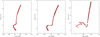Fig. 15.

Evolutionary tracks of the 0.8 (left panel), 1.0 (middle panel), and 2.0 M_⊙ (right panel) stars with chemical composition [X = 0.703, Y = 0.280, Z = 0.017] calculated with the SFCT forced to include the strict pressure balance at the surface of convective elements (dotted red line). The corresponding models with the MLT with mixing length parameter Λ_m = 1.68 (black line) are also shown for comparison. The agreement is beyond any reasonable expectation. The MLT is clearly a particular case of the SFCT.

10. Summary and conclusions

In this section, we briefly summarize the key points of the SFCT, highlight the major achievements, and make some general comments.

(1) Aims. Three simple considerations are the starting motivations of the SFCT: (i) the vast majority of stellar models in literature are calculated with the classical MLT and companion MLP that requires independent and a priori calibrations; (ii) in contrast, highly sophisticated hydrodynamic studies of convection have been developed over the years; however, their complexity hampers the straight application to stellar models; (iii) a few exceptions exist using more sophisticated theories of convection (see e.g., Canuto & Mazzitelli 1991; Canuto et al. 1996 with their full spectrum turbulence models, Xiong 1986, Wuchterl & Feuchtinger 1998, and others with nonlocal models of convection).

Based on this, Pasetto et al. (2014) initiated a series of studies aimed at bridging the gap. The leading idea is to replace the classical MLT with a new theory in which all the convection properties are unambiguously determined by the underlying stellar physics (EOS, chemical composition, mass, and age), and no free parameters are introduced (the SFCT). In view of the future use in stellar models, the whole SFCT has been formulated using the same language, hypotheses, and formalism of the MLT.

(2) Theoretical framework of the SFCT. The stellar medium is a perfect fluid governed by an EOS (that can change with position and time). A convective region is characterized by the following physical quantities: the size ξ_e, velocity v_e, and temperature gradient ∇_e of the generic element, the three gradients of the surrounding medium (adiabatic ∇_ad, fictitious radiative ∇_rad, and ambient ∇), and the convective and radiative fluxes of energy, φ_cnv and ∇_rad, respectively. The complicated motion of a convective element is idealized and simplified as being made of two components: the vertical displacement at a certain velocity v_e = ṙ_e where r_e is the radial coordinate of the element’s center of mass (spherical symmetry of the star is assumed), and expansion or contraction of its size ξ_e at the rate ${\dot{ξ}}_{e}$ $\dot \xi_{\mathrm{e}}$ (spherical shape of the convective elements is also assumed). The extension of a convective region is defined by the well-known stability criteria, either Schwarzschild or Ledoux. All these quantities are functions of position and time.

(3) Basic assumptions of the SFCT. The fluid is assumed to be viscous-free, incompressible on suitable local scales, and irrotational (turbulence free). Consequently, three important assumptions can be made. First, in compliance with Eq. (34), a fundamental theorem of turbulence, the convective elements cannot be in mechanical equilibrium with the surrounding medium during their whole lifetime; that is, the immediate pressure balance at the surface of a generic convective element cannot exist. This means that the complete Bernoulli equation must be used. Contrary to what one may infer from this statement, at any layer of a convective region, the fluid as a whole obeys the condition of hydrostatic equilibrium. The Bernoulli equation of the fluid as a function of time and position is derived by combining the Euler equation with the mass conservation and performing the space integration. The Bernoulli equation, originally formulated in the inertial reference frame with its origin on the star center, is then recast in a polar frame comoving with the convective element and with origin on the element barycenter. The second assumption is that turbulence can be neglected, and hence the velocity field outside the surface of the expanding (contracting) element and inclusive of the vertical and expansion (contraction) motions can be derived from a suitable potential. Finally, the third assumption, based on several arguments, is that the upward (downward) velocity is smaller than the expansion (contraction) velocity $| v | ≪ | {\dot{ξ}}_{e} |$ $\left| \boldsymbol{v}\right| \ll \left| {{\boldsymbol{\dot \xi_{\mathrm{e}} }}} \right|$ . The ratio $ε \equiv | v | / | {\dot{ξ}}_{e} | ≪ 1$ $\varepsilon \equiv{ {\left| {\boldsymbol{v} } \right|}}/{{\left| {{\boldsymbol{\dot \xi_{\mathrm{e}} }}} \right|}} \ll 1$ is then used as a parameter to linearize the Bernoulli equation in the comoving frame.

(4) The expansion (contraction) rate. We derive a dimensionless equation relating the dimensions ξ_e of the element, the rate of expansion (contraction) ${\dot{ξ}}_{e}$ $\dot \xi_{\mathrm{e}}$ , the acceleration of this ${\ddot{ξ}}_{e}$ $\ddot \xi_{\mathrm{e}}$ , and containing the relative acceleration A between the inertial and the comoving frames. The analytical integration of this equation provides a basic relationship between the mean value of the radius and time (both normalized to arbitrary factors). In other words, the equation for the expansion (contraction) of the dimension of the generic convective element is obtained. In addition to this, there are three other important relationships: (i) between the dimensions ξ_e and the velocity v_e of an element; (ii) between the kinetic energy per units mass and the work done by buoyancy forces over a spatial distance equal to the dimension of the convective element, $v_{e}^{2} = A 2 \times ξ_{e}$ ${\it v}_{\rm e}^2 = A\, 2\times \xi_{\rm e}$ . This relation finds its analog in the MLT in which the work done by the buoyancy forces over a certain distance (typically h_p) is used to estimate the velocity of a convective element; and (iii) between the dimension of the element and its radial velocity and time $ξ_{e} = \frac{| v | \sqrt{χ}}{2}$ ${\xi _{\mathrm{e}}} = \frac{{\left| { \mathit{v}} \right|\sqrt \chi }}{2}$ . Six nonlinear equations link them all together. Furthermore, the vertical (radial) component of the relative acceleration A_z is derived. This is the sum of three components: the buoyancy force of the convective element $\frac{4}{3} ξ_{e}^{3} π ρ g$ $\frac{4}{3} \xi_{\mathrm{e}}^3 \pi \rho \boldsymbol{g}$ , the inertial term of the field displaced by the movement of the convective element with reaction mass $\frac{2}{3} π ξ_{e}^{3} ρ$ $\frac{2}{3}\pi \xi_{\mathrm{e}}^3 \rho$ , and a new term $2 π ρ v \dot{ξ_{e}} ξ_{e}^{2}$ $2\pi \rho \mathit{v} \dot{\xi_{\mathrm{e}}} \xi_{\mathrm{e}}^2$ arising from the changing size of the convective element. Finally, A_z is expressed as a function of the temperature gradients ∇ (medium), ∇_e (element), and ∇_μ (molecular weight). All these equations can be used to set up a system of six equations that yields an algebraic equation of fifth degree (the analog of the cubic equation of the MLT) whose solution determines the velocity v and the dimension ξ_e of the generic convective element once the stationary regime is reached (time integration is required and performed). All physical quantities needed to describe convection in the SFCT follow immediately.

(5) Solution uniqueness. The equation contains the time as a variable. Therefore, as already said, time integration is required. Fortunately, the timescales over which a stationary solution is reached are very short, in any case much shorter than any other evolutionary timescale. Once the stationarity condition is reached, the solution provided by the SFCT is unique.

(6) Closure of equations and irrelevance of external parameters. In the SFCT, the convective elements can move radially and expand (contract) simultaneously. In addition to the buoyancy force, the inertia of the fluid displaced by the convective elements and the effect of their expansion on the buoyancy force itself are taken into account. The dynamical aspect of the problem greatly differs with respect to that of the classical MLT, and the resulting equations are sufficient to determine all the properties of stellar convection (velocities, dimensions and temperature gradients of the convective elements, temperature gradients of the medium, and, finally, the energy flux carried by convection) as a function of the environment physics (temperature, density, chemical composition, opacity, etc.), with no need at all for the ML parameter.

(7) Boundary conditions. The SFCT is a dynamical theory, so suitable boundary conditions at the surface layers must be supplied to the system of equations in order to fix the solution. The issue has been examined in great detail. The key steps and results of the analysis are the following. (i) The definition of an empirical 𝔉 function such that the ambient temperature gradient ∇ inside the convective region in the atmosphere is simply given by the product ∇_ad × 𝔉. The 𝔉 function is found to be the same throughout the history of a star of a given mass and also in stars of different mass in the 0.8 to 1.5 M_⊙ interval, in which the 𝔉 function and its effect have been explored. The 𝔉 function shows two sudden changes of slope at the different layers of the external convective envelope of a star. The first knee is at log P ≃ 5.4 dyn cm⁻² (we named it the inversion layer) and at log P ≃ 6 dyn cm⁻². Beyond this boundary, the velocities and ∇ predicted by the SFCT are nearly identical to those of the MLT. From the surface to log P ≃ 6 dyn cm⁻² MLT and SFCT could predict very different results if the boundary conditions are neglected or not carefully determined. In any case, the 𝔉 function is not used in the formulation of the SFCT, even if it has inspired us the analysis of the boundary conditions. (ii) Two timescales can be defined. Firstly, we have the timescale t_asy, to reach the asymptotic regime in the equations governing the convective transport. Secondly, the timescale t_cnv is required by the convective elements to cross the convective regions. The two timescales are used to derive the ratio Π = t_asy/t_cnv, i.e., to set up the boundary conditions. (iii) Moving from the stellar surface to deeper layers, the asymptotic time t_asy first rapidly decreases, reaches a minimum value, and then steadily increases again. The behavior of t_asy is due to the efficiency of mathematical properties of the solution of the quintic equation in varying the integration time and also the position inside the convective region. Remarkably, the layer of minimum t_asy occurs at the same pressure at which the inversion layer of the 𝔉 function and, even more importantly, the minimum of the ratio Π and dimensions of the convective elements ξ_e are located. The timescale t_cnv monotonically increases from the surface to the interiors. The two timescales are used to derive the ratio Π = t_asy/t_cnv. (iv) The minimum of t_asy also determines a minimum in the vertical acceleration of the convective elements and a maximum in the difference ∇ − ∇_e. The minimum in the acceleration coincides also with the minimum in the dimension ξ_e of a convective element and also the layer at which the dimension ξ_e parallels the distance to the surface. (v) The properties of the region comprised between the surface and the inversion layer heavily affect the local temperature gradient of the medium and the effective temperature in turn. Suitable boundary conditions must be supplied for this region. In such a case the ambient temperature gradient ∇ has the same general trend both in the MLT and SFCT, and both peak at the layer of rapid decrease of the adiabatic gradient ∇_ad. Due to this, both theories predict stellar models with nearly identical effective temperature and, therefore, path in the HRD. Consequently, both fit the position of the Sun on the HRD. This cannot be a coincidence, because the stellar models from both theories agree from the zero age main sequence to the bottom of the RGB. The advantage of the SFCT with respect to the MLT is that no ML parameter has to be fixed and calibrated before calculating stellar models. (v) In any case, we can also define the analog of the ML parameter Λ_m of the classical MLT in the case of the SFCT. This allows us to read the results of the SFCT with the language of the classical MLT.

(8) Recovering the MLT. The MLT is a particular case of the SFCT. As a matter of fact, imposing rigorous hydrostatic equilibrium at the surface of convective elements by hand, we recover the results of the MLT. The stellar models calculated with this revision of the SFCT are indistinguishable from those calculated with classical MLT. The net advantage with respect to the classical MLT is that no MLP is required. This is a good point in favor of the SFCT.

(9) Physical meaning of the ML parameter. The MLT captures the essence of the energy transported inside a star to a good approximation. This happens because the MLT contains a free parameter whose meaning is not to merely quantify the distance traveled by an “average” eddy in the vertical direction inside a star, but also to somehow take into account the whole phenomenon of the turbulence cascade of energy, the transmission of the energy to the flux, the interaction between eddies, the complex pressure information transmission from a place to another, and so on. The MLT is not a hydrodynamic theory because no time evolution is considered in it. Therefore, the question of how far a convective element can travel has no simple physical meaning because there is no such simple connection between the average motion of the turbulent eddies and the pressure scale length. The pressure scale length is a natural scale length of a star related to the dynamics of convective elements through Eq. (34), whereas in reality the mixing length has little, if anything at all, to do with a length scale or a radial motion.

(10) Remarks on the key ingredients of the SFCT. Pasetto et al. (2019) critically examined the key ingredient of the SFCT, that is, the treatment of the pressure field surrounding a convective element. In this study, the authors (i) described their view of the pressure field in the SFCT limited to the case of an homogeneous isotropic interstellar plasma and compared it with the MLT; (ii) presented a numerical validation of the SFCT equations with the aid of simple model atmosphere for the external layers of the Sun that complements the analytical treatment of Pasetto et al. (2014); (iii) confuted the arguments brought by Miller Bertolami et al. (2016) against the physical foundations of the SFCT; (iv) obtained the first numerical estimations of the temporal dependence of the onset of full convection in a layer that is unstable according to the classical Schwarzschild or Ledoux criteria, that is, the onset is not instantaneous but takes some time to occur; and (v) highlighted the limitations of the SFCT in relation to the temporal integration and the possible effects of neglecting the presence of turbulence.

(11) Stellar models with the SFCT. The success of the SFCT is evident in the quality of the stellar models it generates, which nicely fit the positions of stars in the HRD by continuously adapting themselves to the ever-changing properties of the star during its evolutionary history and without requiring a side calibration on standard stars such as the Sun. Moreover, the mathematical exploitation of the uniqueness theorem in Pasetto et al. (2014) can open new possibilities not only to eliminate parameters whose nature and physical meaning are far from being clear (e.g., the mixing length), but also to investigate the closure relations of the hierarchy of hydrodynamic equations (e.g., Launder & Sandham 2002). The validity of the SFCT could also be investigated using other techniques such as deep helio-seismology and giro-seismology studies. Nevertheless, the SFCT constitutes a step forward concerning the classical MLT, with which it shares the significant merits of simplicity and easy usage, but which it surpasses by eliminating the so-called mixing length parameter. The SFCT does not intend to replace or compete with more sophisticated theories of convection and 3D numerical simulations that, however, still appear far from ready for use in stellar models.

(12) SFCT vs. MLT; final considerations. For more than seventy years, the vast majority of stellar models in the literature (many thousands of them) have been successfully calculated with the classical MLT. The associated MLP has been calibrated on the Sun or another suitable star. With these stellar models, isochrones and synthetic color-magnitude diagrams have been derived and successfully used to study the stellar content of clusters and galaxies in the local and far Universe. The MLT relies on the Boussinesq approximation, by which convection is described as being made by elements of an undefined shape whose dimensions are roughly equal to the ML itself (via the MLP), travel over a distance roughly equal to their dimensions, and suddenly dissolve to release their residual internal energy. Part of the energy accumulated at the beginning of their history has been radiated away during their lifetime (also, this requires some hidden parameters). The equation of motion is limited to the acceleration imparted by the buoyancy force and gravity, turbulence is neglected, and the mean velocity of the vertical motion is roughly estimated by the work done by the buoyancy forces using the energy conservation principle (a fraction of the work goes into kinetic energy). Once the mean velocity is known, the convective flux is eventually derived. All stellar evolutionists were fully happy with the MLT of stellar convection. In most cases, phenomena like semiconvection, overshooting, and so on, are taken into account by means ad hoc prescriptions and make use of physical quantities including the velocity of convective motions derived from the MLT. In the meantime, other more sophisticated theories of convection (see Canuto & Mazzitelli 1991; Kuhfuß 1986; Xiong 1986, and Canuto & Hartke 1986 to mention a few) and large numerical simulations of turbulent convection have been developed as already amply quoted in this paper. For a complete review of the progress made in all these issues and exhaustive referencing, we invite the reader to consult Kupka & Muthsam (2017). Unfortunately, all the results of these recent achievements could not be easily incorporated into current numerical codes for stellar models and stellar evolutionary sequences because of their complexity, and stellar evolutionists continued to rely on the MLT and the MLP to carry all the calculations. The SFCT tries to improve upon the MLT and to rule out the need of the MLP. The SFCT stands on the same assumptions adopted for the MLT, the only differences being (i) the virtual release of the immediate mechanical equilibrium between convective elements and surrounding medium that leads to a more general Bernoulli equation; (ii) the inclusion of the simultaneous vertical motion and expansion or shrinkage of the convective elements (more realistic description); (iii) the absence of turbulence that, however, is partially compensated by the expansion or contraction of the elements as far as the amount of energy going into vertical motion; (iv) the adoption of the velocity potential formalism that greatly simplifies the equations; and, finally, (v) the SFCT yields identical results to those of the MLT (without using parameters such as the MLP). If the SFCT is wrong, by the same arguments we must admit that the MLT is wrong too.

(13) SFCT vs. observational data: The next step. So far, the evidence that predictions based on SFCT recover astrophysical data is essentially limited to reproducing the luminosity and radius of the present Sun and in a wider context to compare evolutionary tracks for stars with mass in the interval 0.8–2.5 M_⊙ and chemical composition [X = 0.703, Y = 0.280, Z = 0.017] from the main sequence to advanced stages along the RGB calculated with the classical MLT with Λ_m = 1.68 and the SFCT. It is worth recalling that the MLT models are taken from the Padua library of stellar models, isochrones, and single stellar populations (magnitudes and colors) calculated by Bertelli et al. (2008). These models include convective overshooting from the central core and the intermediate convective shell above the H-burning shell if present and as appropriate to the mass of the star. Furthermore, these models with the MLT have been repeatedly tested against observational data (color-magnitude diagrams) for old clusters (open and globular) and field stars, and in studies of stellar population synthesis, see Bertelli et al. (2008) and references therein. Therefore, as long as the Bertelli et al. (2008) models successfully fit the data for stars from the main sequence to the bottom RGB, so do the SCFT models that coincide with the MLT ones in the same mass interval, chemical composition, and evolutionary stage. The problem of the bright RGB where the SFCT models are cooler than the MLT ones of the same luminosity remains. Looking at the case of 1 M_⊙ star at the luminosity log L/L_⊙ = 2.0 (near the last computed model of the SFCT) we have log T_eff = 3.60 (3982 K) for SFCT and log T_eff = 3.63 (4265 K) for MLT, that is, the MLT temperature is hotter by about 284 K than the SFCT temperature at the luminosity of 100 L_⊙. At the bottom of the RGB the temperature difference for stars from 0.8 to 2.0 M_⊙ is virtually zero and tends to increase with the luminosity. In the 2.5 M_⊙ star, the RGB seems to be always cooler by the same factor at any luminosity. The difference of about 284 K, although not very large, is significant. This implies that the SFCT transport of convective energy is somewhat less efficient than the MLT one. It is worth recalling here that the total flux of energy passing through the atmosphere of a star is built deep inside so that it can be considered as constant in the outermost layer and ready to be transported by radiation and convection (conduction can be neglected here). The radiative flux in turn heavily depends on the opacity, a physical quantity still affected by uncertainty; the higher the opacity, the lower is the radiative flux and the higher the flux to be carried by convection. The energy flux to be delivered by convection is in turn shared between two main agents, namely the thermal capacity of the convective elements and the kinetic energy of their motion. As a consequence of this three-player game, the temperature gradient ∇ governing the expansion, and hence the effective temperature of the star, is also uncertain and not simply related to the convection theory at work. SFCT is more complicated than MLT, so tracing back the reason of the RGB discrepancy is not an easy task. Even more difficult is comparing the results for the RGB of the MLT and SFCT to those of the 3D simulations of convection. As far as this latter issue is concerned, the situation can be summarized as follows. Based on earlier studies by Tayar et al. (2017), Salaris et al. (2018), Mosumgaard et al. (2018, 2020) presented 3D-simulation-based predictions of RGBs that are shifted toward higher effective temperatures in comparison with the MLT based tracks with fixed Λ_m. A similar conclusion was reached by Spada et al. (2021) using different calibrations for the MLT from different RHD simulations alongside two different temperature-optical depth T(τ) relations in the atmosphere of a star. Our RGB models from the SFCT are indeed redder than the corresponding ones from the MLT. A direct comparison with observational data of globular clusters where the RGB is well determined is not yet possible because our present chemical composition is best suited to old open clusters in which the RGB is much less evident. To this aim, sets of evolutionary tracks with other chemical compositions must be calculated with the SFCT. A final note about the 3D simulations of convection concerns the extent to which they represent convection in real stars. Surely a much more complex situation than the one of numerical simulations. To conclude, SFCT still needs to be carefully tested against real observational data. Work is in progress to fill the gap. The slope of the RGB is likely the workbench of this test.

Following the opinion of Kupka & Muthsam (2017) that (ex literis), “which price is the lower one (a parameter free model or a physically more complete model with parameters that require calibration) is probably best judged by comparison to observational data and, where possible, advanced hydrodynamic simulations that solve the fundamental equations...provided that the model assumptions made appear acceptable”, although the SFCT has not yet passed the scrutiny, for the arguments above it appears to be on the right track.

¹

The numerical truncated expression for χ(t) is

$\begin{matrix} χ (τ) ≃ 0.083 τ^{2} + 0.407 τ + 0.663, \end{matrix}$ $\begin{aligned} \chi \left( \tau \right) \simeq 0.083 \tau ^2 + 0.407 \tau + 0.663, \end{aligned}$

which is to be used in the final solution below.

²

This paper appeared in ArXiv but was never published.

³

This is identical to Eq. (A18) of Pasetto et al. (2016).

⁴

A note on the notation: here, all the quantities of the SFCT (as well as for the MLT) refer to the average behavior over the layer L. Nevertheless, only for the velocities $\bar{v}$ $\bar {v}$ and the expansion function $\bar{χ}$ $\bar \chi$ do we use an upper bar to distinguish them from the value for a single element in order not to confuse them with the notation of the previous section. The averaging process for $\bar{v}$ $\bar{v}$ and $\bar{χ}$ $\bar{\chi}$ is detailed in Pasetto et al. (2014) and in the next section.

Acknowledgments

We are deeply grateful to the anonymous referee who much helped us with his/her criticism, advice, comments, and practical information to much improve the original version of the manuscript. This work benefited from support by the National Science Foundation under Grant No. PHY-1430152 (JINA Centre for the Evolution of the Elements). C.C. warmly acknowledges the hospitality from the Department of Physics and Astronomy of the Padova University. A package containing all the routines needed to solve the quintic equation, written in Fortran 90 and easy to insert in any evolutionary code for stellar models, can be obtained from the authors upon request.

References

Arnett, W. D., Meakin, C., Viallet, M., et al. 2015, ApJ, 809, 30 [NASA ADS] [CrossRef] [Google Scholar]
Balmforth, N. J. 1992, MNRAS, 255, 603 [NASA ADS] [CrossRef] [Google Scholar]
Batchelor, G. K., & Proudman, I. 1956, Phil. Trans. Royal Soc. London Ser. A, 248, 369 [CrossRef] [Google Scholar]
Bazán, G., & Arnett, D. 1998, ApJ, 496, 316 [CrossRef] [Google Scholar]
Bec, J., Biferale, L., Cencini, M., Lanotte, A. S., & Toschi, F. 2010, J. Fluid Mech., 646, 527 [NASA ADS] [CrossRef] [Google Scholar]
Benzi, R., Biferale, L., Fisher, R., Lamb, D. Q., & Toschi, F. 2010, J. Fluid Mech., 653, 221 [NASA ADS] [CrossRef] [Google Scholar]
Berge, P., & Dubois, M. 1984, Contemp. Phys., 25, 535 [NASA ADS] [CrossRef] [Google Scholar]
Bertelli, G., Girardi, L., Marigo, P., & Nasi, E. 2008, A&A, 484, 815 [NASA ADS] [CrossRef] [EDP Sciences] [Google Scholar]
Biermann, L. 1932, Z. Astrophys., 5, 117 [NASA ADS] [Google Scholar]
Biermann, L. 1951, Z. Astrophys., 28, 304 [NASA ADS] [Google Scholar]
Bodenschatz, E., Pesch, W., & Ahlers, G. 2000, Ann. Rev. Fluid Mech., 32, 709 [NASA ADS] [CrossRef] [Google Scholar]
Böhm-Vitense, E. 1958, Z. Astrophys., 46, 108 [Google Scholar]
Brown, T. M., & Gilliland, R. L. 1994, ARA&A, 32, 37 [NASA ADS] [CrossRef] [Google Scholar]
Brown, T. M., Ferguson, H. C., Smith, E., et al. 2005, AJ, 130, 1693 [Google Scholar]
Cantin, N., Vincent, A. P., & Yuen, D. A. 2000, Geophys. J. Int., 140, 163 [NASA ADS] [CrossRef] [Google Scholar]
Canuto, V. M. 2007a, in Convection in Astrophysics, eds. F. Kupka, I. Roxburgh, & K. L. Chan, 239, 3 [NASA ADS] [Google Scholar]
Canuto, V. M. 2007b, in Convection in Astrophysics, eds. F. Kupka, I. Roxburgh, & K. L. Chan, 239, 19 [NASA ADS] [Google Scholar]
Canuto, V. M. 2011a, A&A, 528, A76 [NASA ADS] [CrossRef] [EDP Sciences] [Google Scholar]
Canuto, V. M. 2011b, A&A, 528, A77 [NASA ADS] [CrossRef] [EDP Sciences] [Google Scholar]
Canuto, V. M. 2011c, A&A, 528, A78 [NASA ADS] [CrossRef] [EDP Sciences] [Google Scholar]
Canuto, V. M. 2011d, A&A, 528, A79 [NASA ADS] [CrossRef] [EDP Sciences] [Google Scholar]
Canuto, V. M. 2011e, A&A, 528, A80 [NASA ADS] [CrossRef] [EDP Sciences] [Google Scholar]
Canuto, V. M., & Hartke, G. J. 1986, A&A, 168, 89 [NASA ADS] [Google Scholar]
Canuto, V. M., & Mazzitelli, I. 1991, ApJ, 370, 295 [NASA ADS] [CrossRef] [Google Scholar]
Canuto, V. M., & Mazzitelli, I. 1992, ApJ, 389, 724 [NASA ADS] [CrossRef] [Google Scholar]
Canuto, V. M., Goldman, I., & Mazzitelli, I. 1996, ApJ, 473, 550 [NASA ADS] [CrossRef] [Google Scholar]
Cassisi, S. 2017, Eur. Phys. J. Web Conf., 160, 04002 [Google Scholar]
Cassisi, S., Salaris, M., & Pietrinferni, A. 2016, Mem. Soc. Astron. Ital., 87, 332 [Google Scholar]
Chaplin, W. J. 2013, ASP Conf. Ser., 478, 101 [NASA ADS] [Google Scholar]
Chaplin, W. J., & Miglio, A. 2013, ARA&A, 51, 353 [Google Scholar]
Chiavassa, A., Bigot, L., Thévenin, F., et al. 2011, J. Phys. Conf. Ser., 328, 012012 [NASA ADS] [CrossRef] [Google Scholar]
Christensen-Dalsgaard, J. 2002, Rev. Mod. Phys., 74, 1073 [Google Scholar]
Collet, R., Magic, Z., & Asplund, M. 2011, J. Phys. Conf. Ser., 328, 012003 [NASA ADS] [CrossRef] [Google Scholar]
Couch, S. M., Chatzopoulos, E., Arnett, W. D., & Timmes, F. X. 2015, ApJ, 808, L21 [NASA ADS] [CrossRef] [Google Scholar]
Cox, J. P., & Giuli, R. T. 1968, Principles of Stellar Structure - Vol. 1: Physical Principles; Vol. 2: Applications to Stars [Google Scholar]
Cristini, A., Meakin, C., Hirschi, R., et al. 2017, MNRAS, 471, 279 [NASA ADS] [CrossRef] [Google Scholar]
da Silva, C. B., Hunt, J. C. R., Eames, I., & Westerweel, J. 2014, Ann. Rev. Fluid Mech., 46, 567 [NASA ADS] [CrossRef] [Google Scholar]
Deng, L., & Xiong, D. R. 2008, IAU Symp., 252, 83 [NASA ADS] [CrossRef] [Google Scholar]
Deng, L., Xiong, D. R., & Chan, K. L. 2006, ApJ, 643, 426 [NASA ADS] [CrossRef] [Google Scholar]
Flaskamp, M. 2003, PhD thesis, TU München (Germany) [Google Scholar]
Frisch, U. 1998, Astrophys. Lett. Commun., 35, 463 [NASA ADS] [Google Scholar]
Gastine, T., Wicht, J., & Aurnou, J. M. 2015, J. Fluid Mech., 778, 721 [NASA ADS] [CrossRef] [Google Scholar]
Glatzmaier, G. A. 2013, Introduction to Modelling Convection in Planets and Stars (Princeton: Princeton University Press) [Google Scholar]
Goluskin, D., & van der Poel, E. P. 2016, J. Fluid Mech., 791, R6 [NASA ADS] [CrossRef] [Google Scholar]
Gough, D. O. 1969, J. Atmos. Sci., 26, 448 [NASA ADS] [CrossRef] [Google Scholar]
Grossman, S. A. 1996, MNRAS, 279, 305 [NASA ADS] [CrossRef] [Google Scholar]
Horst, L., Edelmann, P. V. F., Andrássy, R., et al. 2020, A&A, 641, A18 [NASA ADS] [CrossRef] [EDP Sciences] [Google Scholar]
Hotta, H., Rempel, M., & Yokoyama, T. 2015, ApJ, 798, 51 [Google Scholar]
Houdek, G., & Dupret, M.-A. 2015, Liv. Rev. Sol. Phys., 12, 8 [Google Scholar]
Ishihara, T., Gotoh, T., & Kaneda, Y. 2009, Ann. Rev. Fluid Mech., 41, 165 [NASA ADS] [CrossRef] [Google Scholar]
Jackson, J. D. 1975, Classical Electrodynamics (New York: John Wiley& Sons, Inc.) [Google Scholar]
Jenkins, M., & Traub 1970, J. Numer. Math, 14, 252 [CrossRef] [Google Scholar]
Jiang, Y.-F., Cantiello, M., Bildsten, L., Quataert, E., & Blaes, O. 2015, ApJ, 813, 74 [Google Scholar]
Jin, J., Zhu, C., & Lü, G. 2015, PASJ, 67, 19 [NASA ADS] [CrossRef] [Google Scholar]
Johnston, H., & Doering, C. R. 2009, Phys. Rev. Lett., 102, 064501 [NASA ADS] [CrossRef] [Google Scholar]
Joyce, M., & Tayar, J. 2023, Galaxies, 11, 75 [NASA ADS] [CrossRef] [Google Scholar]
Käpylä, P. J. 2019, A&A, 631, A122 [NASA ADS] [CrossRef] [EDP Sciences] [Google Scholar]
Käpylä, P. J. 2021, A&A, 655, A78 [NASA ADS] [CrossRef] [EDP Sciences] [Google Scholar]
Käpylä, P. J. 2023, A&A, 669, A98 [NASA ADS] [CrossRef] [EDP Sciences] [Google Scholar]
Kippenhahn, R., & Weigert, A. 1994, Stellar Structure and Evolution (Berlin: Springer) [Google Scholar]
Kippenhahn, R., Weigert, A., & Weiss, A. 2012, Stellar Structure and Evolution (Berlin: Springer) [Google Scholar]
Kitiashvili, I. N., Kosovichev, A. G., Mansour, N. N., & Wray, A. A. 2016, ApJ, 821, L17 [NASA ADS] [CrossRef] [Google Scholar]
Kochukhov, O., Freytag, B., Piskunov, N., & Steffen, M. 2007, in Convection in Astrophysics, eds. F. Kupka, I. Roxburgh, & K. L. Chan, 239, 68 [NASA ADS] [Google Scholar]
Kolmogorov, A. 1941, Akademiia Nauk SSSR Doklady, 30, 301 [Google Scholar]
Kueker, M., Ruediger, G., & Kitchatinov, L. L. 1993, A&A, 279, L1 [NASA ADS] [Google Scholar]
Kuhfuß, R. 1986, A&A, 160, 116 [NASA ADS] [Google Scholar]
Kuhfuß, R. 1987, PhD thesis, TU München (Germany) [Google Scholar]
Kupka, F., & Muthsam, H. J. 2017, Liv. Rev. Comput. Astrophys., 3, 1 [Google Scholar]
Landau, L. D., & Lifshitz, E. M. 1959, Fluid Mechanics (Oxford: Pergamon Press) [Google Scholar]
Launder, B. E., & Sandham, N. D. 2002, Closure Strategies for Turbulent and Transitional Flows (Cambridge: Cambridge University Press), 768 [Google Scholar]
Lecoanet, D., Schwab, J., Quataert, E., et al. 2016, ApJ, 832, 71 [NASA ADS] [CrossRef] [Google Scholar]
Lohse, D., & Xia, K.-Q. 2010, Ann. Rev. Fluid Mech., 42, 335 [NASA ADS] [CrossRef] [Google Scholar]
Ludwig, H.-G., Jordan, S., & Steffen, M. 1994, A&A, 284, 105 [NASA ADS] [Google Scholar]
Ludwig, H.-G., Freytag, B., & Steffen, M. 1999, A&A, 346, 111 [Google Scholar]
Lydon, T. J., Fox, P. A., & Sofia, S. 1992, ApJ, 397, 701 [NASA ADS] [CrossRef] [Google Scholar]
Magic, Z. 2016, A&A, 586, A88 [NASA ADS] [CrossRef] [EDP Sciences] [Google Scholar]
Magic, Z., Collet, R., & Asplund, M. 2013a, in EAS Publications Series, 63, 367 [NASA ADS] [CrossRef] [EDP Sciences] [Google Scholar]
Magic, Z., Collet, R., Asplund, M., et al. 2013b, A&A, 557, A26 [NASA ADS] [CrossRef] [EDP Sciences] [Google Scholar]
Magic, Z., Collet, R., Asplund, M., et al. 2013c, A&A, 560, A8 [NASA ADS] [CrossRef] [EDP Sciences] [Google Scholar]
Magic, Z., Weiss, A., & Asplund, M. 2015, A&A, 573, A89 [NASA ADS] [CrossRef] [EDP Sciences] [Google Scholar]
Meakin, C. A., & Arnett, D. 2007, ApJ, 667, 448 [NASA ADS] [CrossRef] [Google Scholar]
Meneveau, C. 2011, Ann. Rev. Fluid Mech., 43, 219 [NASA ADS] [CrossRef] [Google Scholar]
Miller Bertolami, M. M., Viallet, M., Prat, V., Barsukow, W., & Weiss, A. 2016, MNRAS, 457, 4441 [CrossRef] [Google Scholar]
Moeng, C.-H., & Rotunno, R. 1990, J. Atmos. Sci., 47, 1149 [NASA ADS] [CrossRef] [Google Scholar]
Moravveji, E., Townsend, R. H. D., Aerts, C., & Mathis, S. 2016, ApJ, 823, 130 [NASA ADS] [CrossRef] [Google Scholar]
Mosumgaard, J. R., Ball, W. H., Silva Aguirre, V., Weiss, A., & Christensen-Dalsgaard, J. 2018, MNRAS, 478, 5650 [NASA ADS] [CrossRef] [Google Scholar]
Mosumgaard, J. R., Jørgensen, A. C. S., Weiss, A., Silva Aguirre, V., & Christensen-Dalsgaard, J. 2020, MNRAS, 491, 1160 [Google Scholar]
Muthsam, H. J., & Kupka, F. 2016, Commmun. Konkoly Obs. Hungary, 105, 117 [NASA ADS] [Google Scholar]
Nordlund, Å., Stein, R. F., & Asplund, M. 2009, Liv. Rev. Sol. Phys., 6, 2 [Google Scholar]
Pandey, A., Scheel, J. D., & Schumacher, J. 2018, Nat. Commun., 9, 2118 [NASA ADS] [CrossRef] [Google Scholar]
Pasetto, S., Chiosi, C., Cropper, M., & Grebel, E. K. 2014, MNRAS, 445, 3592 [NASA ADS] [CrossRef] [Google Scholar]
Pasetto, S., Chiosi, C., Chiosi, E., Cropper, M., & Weiss, A. 2016, MNRAS, 459, 3182 [CrossRef] [Google Scholar]
Pasetto, S., Chiosi, C., Cropper, M., Chiosi, E., & Crnojevic, D. 2019, ArXiv e-prints [arXiv:1909.13513] [Google Scholar]
Pinheiro, F. J. G., & Fernandes, J. 2013, MNRAS, 433, 2893 [NASA ADS] [CrossRef] [Google Scholar]
Piper, M., Wyngaard, J. C., Snyder, W. H., & Lawson, R. E., Jr 1995, J. Atmos. Sci., 52, 3607 [NASA ADS] [CrossRef] [Google Scholar]
Plesset, M. S. 1954, J. Appl. Phys., 25, 96 [NASA ADS] [CrossRef] [Google Scholar]
Pope, S. B. 2000, Turbulent Flows (Cambridge: Cambridge University Press), 806 [Google Scholar]
Porter, D. H., & Woodward, P. R. 2000, ApJS, 127, 159 [NASA ADS] [CrossRef] [Google Scholar]
Prandtl, L. 1925, Math, Meth., 5, 136 [NASA ADS] [Google Scholar]
Press, W. H., Teukolsky, S. A., Vetterling, W. T., & Flannery, B. P. 1992, Numerical Recipes in FORTRAN. The Art of Scientific Computing (Cambridge: Cambridge University Press) [Google Scholar]
Rampazzo, R., D’Onofrio, M., Zaggia, S., et al. 2016, Astrophys. Space Sci. Lib., 435, 1 [NASA ADS] [CrossRef] [Google Scholar]
Rempel, M., & Cheung, M. C. M. 2014, ApJ, 785, 90 [Google Scholar]
Rieutord, M., & Rincon, F. 2010, Liv. Rev. Sol. Phys., 7, 2 [Google Scholar]
Rogers, T. M., Glatzmaier, G. A., & Woosley, S. E. 2003, Phys. Rev. E, 67, 026315 [CrossRef] [Google Scholar]
Rosenthal, C. S., Christensen-Dalsgaard, J., Nordlund, Å., Stein, R. F., & Trampedach, R. 1999, A&A, 351, 689 [NASA ADS] [Google Scholar]
Saffman, P. G. 1967, J. Fluid Mech., 27, 581 [Google Scholar]
Salaris, M., & Cassisi, S. 2015, A&A, 577, A60 [CrossRef] [EDP Sciences] [Google Scholar]
Salaris, M., Cassisi, S., Schiavon, R. P., & Pietrinferni, A. 2018, A&A, 612, A68 [NASA ADS] [CrossRef] [EDP Sciences] [Google Scholar]
Schmidt, W., & Federrath, C. 2011, A&A, 528, A106 [NASA ADS] [CrossRef] [EDP Sciences] [Google Scholar]
Schumacher, J., Scheel, J. D., Krasnov, D., et al. 2014, Proc. Natl. Acad. Sci., 111, 10961 [NASA ADS] [CrossRef] [Google Scholar]
Schumann, U. 1993, J. Atmos. Sci., 50, 116 [NASA ADS] [CrossRef] [Google Scholar]
Smalley, B., & Kupka, F. 1997, A&A, 328, 349 [NASA ADS] [Google Scholar]
Spada, F., Demarque, P., & Kupka, F. 2021, MNRAS, 504, 3128 [NASA ADS] [CrossRef] [Google Scholar]
Spiegel, E. A., & Veronis, G. 1960, ApJ, 131, 442 [NASA ADS] [CrossRef] [Google Scholar]
Stancliffe, R. J. 2016, IAU Focus Meet., 29B, 600 [Google Scholar]
Stancliffe, R. J., Fossati, L., Passy, J. C., & Schneider, F. R. N. 2016, A&A, 586, A119 [NASA ADS] [CrossRef] [EDP Sciences] [Google Scholar]
Stein, R. F., & Nordlund, Å. 2000, Sol. Phys., 192, 91 [NASA ADS] [CrossRef] [Google Scholar]
Stevens, R. J. A. M., Blass, A., Zhu, X., Verzicco, R., & Lohse, D. 2018, Phy. Rev. Fluids, 3, 041501 [NASA ADS] [CrossRef] [Google Scholar]
Tayar, J., Somers, G., Pinsonneault, M. H., et al. 2017, ApJ, 840, 17 [NASA ADS] [CrossRef] [Google Scholar]
Trampedach, R., Asplund, M., Collet, R., Nordlund, Å., & Stein, R. F. 2013, ApJ, 769, 18 [NASA ADS] [CrossRef] [Google Scholar]
Tuteja, G. S., Khattar, D., Chakraborty, B. B., & Bansal, S. 2010, Int. J. Contemp. Math. Sci., 5, 1065 [Google Scholar]
Ulrich, R. K., & Rhodes, E. J., Jr 1977, ApJ, 218, 521 [NASA ADS] [CrossRef] [Google Scholar]
Vincent, A. P., & Yuen, D. A. 1999, Phys. Rev. E, 60, 2957 [NASA ADS] [CrossRef] [Google Scholar]
Vincent, A. P., & Yuen, D. A. 2000, Phys. Rev. E, 61, 5241 [NASA ADS] [CrossRef] [Google Scholar]
Vitense, E. 1953, Z. Astrophys., 32, 135 [NASA ADS] [Google Scholar]
Warnecke, J., Rheinhardt, M., Viviani, M., et al. 2021, ApJ, 919, L13 [NASA ADS] [CrossRef] [Google Scholar]
Weiss, A., & Flaskamp, M. 2007, IAU Symp., 239, 314 [NASA ADS] [Google Scholar]
Weiss, A., Hillebrandt, W., Thomas, H.-C., & Ritter, H. 2004, Cox and Giuli’s Principles of Stellar Structure (Cambridge: Cambridge Scientific Publishers) [Google Scholar]
Wuchterl, G., & Feuchtinger, M. U. 1998, A&A, 340, 419 [NASA ADS] [Google Scholar]
Wyngaard, J. C. 1987, J. Atmos. Sci., 44, 1083 [NASA ADS] [CrossRef] [Google Scholar]
Wyngaard, J. C., & Weil, J. C. 1991, Phys. Fluids A, 3, 155 [CrossRef] [Google Scholar]
Xiong, D.-R. 1986, A&A, 167, 239 [NASA ADS] [Google Scholar]
Zhu, X., Mathai, V., Stevens, R. J. A. M., Verzicco, R., & Lohse, D. 2018, Phys. Rev. Lett., 120, 144502 [NASA ADS] [CrossRef] [Google Scholar]
Zingale, M., Malone, C. M., Nonaka, A., Almgren, A. S., & Bell, J. B. 2015, ApJ, 807, 60 [NASA ADS] [CrossRef] [Google Scholar]

All Tables

Table 1.

Most external layers of the atmosphere of the model with chemical composition [X = 0.703, Y = 0.280, Z = 0.017], log L/L_⊙ = 0. log T_eff = 3.762, age = 4.6 Gyr best reproducing the position of the Sun in the HR diagram.

In the text

Table 2.

Same as in Table 1, but for the model along the RGB with log L/L_⊙ = 1.489, log T_eff = 3.638, and age of ≃11 Gyr.

In the text

All Figures

Fig. 1.

Schematic representation of a convective element seen in the inertial frame S_O (origin at the point O) and in the co-moving frame S₁ (origin at the point O′). The element is represented as a spherical body for simplicity. The center of the sphere indicated as O′ also corresponds to the position of the element in S₀. The generic dimension of the convective element as seen in S₁ is indicated by ξ_e. Reproduced from Pasetto et al. (2016).

In the text

Fig. 2.

Artistic representation of temporal evolution of a convective element. The star is a superposition of m layers in hydrostatic equilibrium. The generic layer, L_n, is defined by the hydrostatic pressure, density, and temperature (p,ρ,T)_{L_n}. These values are assumed to be time-independent and far away from the convective element, i.e., for every layer $(p^{\infty}, ρ^{\infty}, T^{\infty}) = {(p, ρ, T)}_{L_{n}} \forall t$ $\left( {{p}^{\infty }},{{\rho }^{\infty }},{{T}^{\infty }} \right)={{\left( p,\rho ,T \right)}_{{{L}_{n}}}}\forall t$ . Vice versa, each convective element is never in hydrostatic equilibrium with its medium, and the pressure, temperature, and density at the surface of a convective element are {p_e(t),ρ_e(t),T_e(t)}≠{p^∞,ρ^∞,T^∞}. Upper and lower borders of a layer are indicated by ∂L_n = ∂L_n(x). Data are from Pasetto et al. (2019).

In the text

Fig. 3.

Temporal and spatial evolution of relative pressure ratio between the value at the surface of a convective element and the one at infinity. Time runs from τ = 0 to τ = 2 from the bottom to the top. The lines start at the surface of a generic spherical element whose position and dimensions grow with time. The radius increases according to Eq. (40). The curves starting from the surface of the different spheres show the variation of the relative pressure difference moving far away from the surface of the element to large distances. The lines refer to the case of a fluid in the irrotational potential-flow approximation. The dashed line shows (limited to one case) the expected variation for a rotational flow. The disintegration of any generic convective element as time goes on is mimicked here by drawing the spheres and lines with progressively less intense colors. Data are taken from Pasetto et al. (2019).

In the text

	Fig. 4. Same as in Fig. 3, but for the velocity field surrounding the eddy. Data are taken from Pasetto et al. (2019).
In the text

Fig. 5.

Run of Π and characteristic timescales of convection in the most external layers of a low-mass star. Left panel: profile of Π across the atmosphere of the MS model of the 1.0 M_⊙ star with chemical composition [X = 0.703, Y = 0.280, Z = 0.017]. We note the fall of Π to the minimum value followed by the rapid increase to Π = 1 at increasing pressure. Right panel: run of the asymptotic time t_asy and convective time t_cnv as a function of log P in the atmosphere of the 1.0 M_⊙ at the Sun’s position (log L/L_⊙ = 0 and log T_eff = 3.762). The asymptotic time has a minimum at the position log P ≃ 5.4, roughly coincident with the adiabatic fall layer. This trend is the remote cause of the minimum in the ratio Π of the left panel, and it is related to the mathematical behavior of the real solutions of the quintic equation in the outermost layer of the external convection (see Fig. 3 of Pasetto et al. 2016). Data are from Pasetto et al. (2016).

In the text

Fig. 6.

Velocity and temperature gradients in SFCT stellar models with the old boundary conditions of Pasetto et al. (2016). Left panel: profile of the convective velocity as function of the pressure across the atmosphere of the 1.0 M_⊙ star with chemical composition [X = 0.703, Y = 0.280, Z = 0.017] at the Sun’s position (log L/L_⊙ = 0 and log T_eff = 3.762). The new boundary conditions are applied for log P ≤ 6.0. Three profiles are shown: the one from the MLT (black line), the one from the SFCT with the new boundary conditions (red dashed lines), and the one from the SFCT with the old boundary conditions (blue dotted line). Right panel: same as left panel, but for temperature gradient of the medium, ∇. Data are from Pasetto et al. (2016).

In the text

	Fig. 7. Evolutionary tracks of 0.8, 1.0, 1.5, 2.0, and 2.5 M_⊙ stars calculated with the MLT (mixing length parameter Λ = 1.68) indicated by crosses and the SFCT indicated by the solid lines of different colors. The comparison shows that the SFCT with no mixing length parameter is equivalent to the classical MLT with calibrated mixing length parameter. Data are from Pasetto et al. (2016).
In the text

Fig. 8.

Profiles of 𝔉 function, adiabatic temperature gradient ∇_ad, and ionization degrees of HI, HeI, and HeII in the external regions of a low-mass star. Left panel: profile of the 𝔉 function as a function of log P in the outer atmospheres of the 1.0 M_⊙ with chemical composition [X = 0.703, Y = 0.280, Z = 0.017] calculated with the MLT from the main sequence to late stages along the RGB. The adopted mixing length parameter is Λ = 1.68. The pressure is in dyn cm⁻². We highlight the two characteristic layers at log P = 5.4 and log P ≃ 6.0, where the 𝔉 function suddenly changes slope (see the text for more details). Right panel: run of adiabatic temperature gradient ∇_ad and ionization degree of HI, HeI, and HeII indicated by y_HI, y_HeI, and y_HeII, respectively, as a function of log P in dyn cm⁻². The drop off of ∇_ad at log P ≃ 5.4 coincides with the start of the HI ionization.

In the text

Fig. 9.

Profiles of dimensions and acceleration of convective elements across the most external convective region of a low mass star. Left panel: dimension reached by the convective elements at t_asy as a function of log P. Since t_asy decreases, the velocity and dimensions of the convective elements in these very external layers are also expected to decrease going toward the adiabatic fall layer. Right panel: radial acceleration of a convective element as a function of the depth (log P) across the external convective zone of the stellar models representing the Sun (thin solid lines with triangles). With respect to the layer of the adiabatic fall (at log P = 5.4 dyn cm⁻²), the left branch of the curve (red triangles) is for ξ_e > D, i.e., Eq. (51), whereas the right branch (blue triangles) is for ξ_e < D, i.e., Eq. (52), and the minimum of the acceleration “coincides” with the value of ≃300 cm s⁻² given by the SFCT, see Eq. (50). The horizontal dotted line is the nearly constant acceleration from the MLT.

In the text

	Fig. 10. Profiles of Π, Π′, and difference ∇ − ∇_e across the most external convective regions of a low-mass star. Left panel: ratios Π and Π′ are compared and found in good qualitative agreement. Right panel: difference ∇ − ∇_e as a function of position (log P). The maximum difference between the two gradients occurs at the layer of the adiabatic fall.
In the text

Fig. 11.

Velocity and temperature gradients in SFCT stellar models with the new boundary conditions discussed in this paper. Left panel: velocity profile in the outer layers. Right panel: Temperature gradient of the medium ∇ in the same region. Both are displayed as a function of log P in the atmosphere of the 1.0 M_⊙ at the Sun’s position (log L/L_⊙ = 0 and log T_eff = 3.762). The new boundary conditions are applied for log P ≤ 6.0. In both panels we show the results for the MLT and SFCT as indicated.

In the text

Fig. 12.

Evolutionary tracks of 1.0 M_⊙ star with chemical composition [X = 0.703, Y = 0.280, Z = 0.017] calculated with the SFCT and the new boundary conditions (red dots) and the old boundary conditions (blue squares) and the MLT with Λ_m = 1.68 (black crosses). The SFCT models with the old and new boundary conditions fully overlap each other. No significant difference is found among the three cases from the main sequence up to the bottom of the RGB. As already noticed by Pasetto et al. (2016), the RGB with the SFCT is more inclined compared to the correspondent one obtained from the MLT (see the text for more details on this issue).

In the text

	Fig. 13. Evolution of averaged fluxes, gradients, and velocity for a 1 M_⊙ stellar model with log₁₀L/L_⊙ = 0.0, log₁₀T_eff = 3.76 and solar metallicity. Left panel refers to R = 0.7 R_⊙, right panel to R = 0.88 R_⊙. Data are from Pasetto et al. (2019).
In the text

Fig. 14.

Numerical validation of Lemma 1 in Pasetto et al. (2014). The functions g,f, and k are defined in the text and plotted against the values of interest in the Lemma 1, i.e., in the “asymptotic” regime of validity of the uniqueness theorem. Evidently, the blue manifold always remains above the green and yellow ones for all the timescales of interest and for any angular dependence of the equations. This temporal interval covers all the stars calculated by Pasetto et al. (2016). Data are from Pasetto et al. (2019).

In the text

Fig. 15.

Evolutionary tracks of the 0.8 (left panel), 1.0 (middle panel), and 2.0 M_⊙ (right panel) stars with chemical composition [X = 0.703, Y = 0.280, Z = 0.017] calculated with the SFCT forced to include the strict pressure balance at the surface of convective elements (dotted red line). The corresponding models with the MLT with mixing length parameter Λ_m = 1.68 (black line) are also shown for comparison. The agreement is beyond any reasonable expectation. The MLT is clearly a particular case of the SFCT.

In the text

Current usage metrics show cumulative count of Article Views (full-text article views including HTML views, PDF and ePub downloads, according to the available data) and Abstracts Views on Vision4Press platform.

Data correspond to usage on the plateform after 2015. The current usage metrics is available 48-96 hours after online publication and is updated daily on week days.

Initial download of the metrics may take a while.

[1] Arnett, W. D., Meakin, C., Viallet, M., et al. 2015, ApJ, 809, 30 [NASA ADS] [CrossRef] [Google Scholar]

[2] Balmforth, N. J. 1992, MNRAS, 255, 603 [NASA ADS] [CrossRef] [Google Scholar]

[3] Batchelor, G. K., & Proudman, I. 1956, Phil. Trans. Royal Soc. London Ser. A, 248, 369 [CrossRef] [Google Scholar]

[4] Bazán, G., & Arnett, D. 1998, ApJ, 496, 316 [CrossRef] [Google Scholar]

[5] Bec, J., Biferale, L., Cencini, M., Lanotte, A. S., & Toschi, F. 2010, J. Fluid Mech., 646, 527 [NASA ADS] [CrossRef] [Google Scholar]

[6] Benzi, R., Biferale, L., Fisher, R., Lamb, D. Q., & Toschi, F. 2010, J. Fluid Mech., 653, 221 [NASA ADS] [CrossRef] [Google Scholar]

[7] Berge, P., & Dubois, M. 1984, Contemp. Phys., 25, 535 [NASA ADS] [CrossRef] [Google Scholar]

[8] Bertelli, G., Girardi, L., Marigo, P., & Nasi, E. 2008, A&A, 484, 815 [NASA ADS] [CrossRef] [EDP Sciences] [Google Scholar]

[9] Biermann, L. 1932, Z. Astrophys., 5, 117 [NASA ADS] [Google Scholar]

[10] Biermann, L. 1951, Z. Astrophys., 28, 304 [NASA ADS] [Google Scholar]

[11] Bodenschatz, E., Pesch, W., & Ahlers, G. 2000, Ann. Rev. Fluid Mech., 32, 709 [NASA ADS] [CrossRef] [Google Scholar]

[12] Böhm-Vitense, E. 1958, Z. Astrophys., 46, 108 [Google Scholar]

[13] Brown, T. M., & Gilliland, R. L. 1994, ARA&A, 32, 37 [NASA ADS] [CrossRef] [Google Scholar]

[14] Brown, T. M., Ferguson, H. C., Smith, E., et al. 2005, AJ, 130, 1693 [Google Scholar]

[15] Cantin, N., Vincent, A. P., & Yuen, D. A. 2000, Geophys. J. Int., 140, 163 [NASA ADS] [CrossRef] [Google Scholar]

[16] Canuto, V. M. 2007a, in Convection in Astrophysics, eds. F. Kupka, I. Roxburgh, & K. L. Chan, 239, 3 [NASA ADS] [Google Scholar]

[17] Canuto, V. M. 2007b, in Convection in Astrophysics, eds. F. Kupka, I. Roxburgh, & K. L. Chan, 239, 19 [NASA ADS] [Google Scholar]

[18] Canuto, V. M. 2011a, A&A, 528, A76 [NASA ADS] [CrossRef] [EDP Sciences] [Google Scholar]

[19] Canuto, V. M. 2011b, A&A, 528, A77 [NASA ADS] [CrossRef] [EDP Sciences] [Google Scholar]

[20] Canuto, V. M. 2011c, A&A, 528, A78 [NASA ADS] [CrossRef] [EDP Sciences] [Google Scholar]

[21] Canuto, V. M. 2011d, A&A, 528, A79 [NASA ADS] [CrossRef] [EDP Sciences] [Google Scholar]

[22] Canuto, V. M. 2011e, A&A, 528, A80 [NASA ADS] [CrossRef] [EDP Sciences] [Google Scholar]

[23] Canuto, V. M., & Hartke, G. J. 1986, A&A, 168, 89 [NASA ADS] [Google Scholar]

[24] Canuto, V. M., & Mazzitelli, I. 1991, ApJ, 370, 295 [NASA ADS] [CrossRef] [Google Scholar]

[25] Canuto, V. M., & Mazzitelli, I. 1992, ApJ, 389, 724 [NASA ADS] [CrossRef] [Google Scholar]

[26] Canuto, V. M., Goldman, I., & Mazzitelli, I. 1996, ApJ, 473, 550 [NASA ADS] [CrossRef] [Google Scholar]

[27] Cassisi, S. 2017, Eur. Phys. J. Web Conf., 160, 04002 [Google Scholar]

[28] Cassisi, S., Salaris, M., & Pietrinferni, A. 2016, Mem. Soc. Astron. Ital., 87, 332 [Google Scholar]

[29] Chaplin, W. J. 2013, ASP Conf. Ser., 478, 101 [NASA ADS] [Google Scholar]

[30] Chaplin, W. J., & Miglio, A. 2013, ARA&A, 51, 353 [Google Scholar]

[31] Chiavassa, A., Bigot, L., Thévenin, F., et al. 2011, J. Phys. Conf. Ser., 328, 012012 [NASA ADS] [CrossRef] [Google Scholar]

[32] Christensen-Dalsgaard, J. 2002, Rev. Mod. Phys., 74, 1073 [Google Scholar]

[33] Collet, R., Magic, Z., & Asplund, M. 2011, J. Phys. Conf. Ser., 328, 012003 [NASA ADS] [CrossRef] [Google Scholar]

[34] Couch, S. M., Chatzopoulos, E., Arnett, W. D., & Timmes, F. X. 2015, ApJ, 808, L21 [NASA ADS] [CrossRef] [Google Scholar]

[35] Cox, J. P., & Giuli, R. T. 1968, Principles of Stellar Structure - Vol. 1: Physical Principles; Vol. 2: Applications to Stars [Google Scholar]

[36] Cristini, A., Meakin, C., Hirschi, R., et al. 2017, MNRAS, 471, 279 [NASA ADS] [CrossRef] [Google Scholar]

[37] da Silva, C. B., Hunt, J. C. R., Eames, I., & Westerweel, J. 2014, Ann. Rev. Fluid Mech., 46, 567 [NASA ADS] [CrossRef] [Google Scholar]

[38] Deng, L., & Xiong, D. R. 2008, IAU Symp., 252, 83 [NASA ADS] [CrossRef] [Google Scholar]

[39] Deng, L., Xiong, D. R., & Chan, K. L. 2006, ApJ, 643, 426 [NASA ADS] [CrossRef] [Google Scholar]

[40] Flaskamp, M. 2003, PhD thesis, TU München (Germany) [Google Scholar]

[41] Frisch, U. 1998, Astrophys. Lett. Commun., 35, 463 [NASA ADS] [Google Scholar]

[42] Gastine, T., Wicht, J., & Aurnou, J. M. 2015, J. Fluid Mech., 778, 721 [NASA ADS] [CrossRef] [Google Scholar]

[43] Glatzmaier, G. A. 2013, Introduction to Modelling Convection in Planets and Stars (Princeton: Princeton University Press) [Google Scholar]

[44] Goluskin, D., & van der Poel, E. P. 2016, J. Fluid Mech., 791, R6 [NASA ADS] [CrossRef] [Google Scholar]

[45] Gough, D. O. 1969, J. Atmos. Sci., 26, 448 [NASA ADS] [CrossRef] [Google Scholar]

[46] Grossman, S. A. 1996, MNRAS, 279, 305 [NASA ADS] [CrossRef] [Google Scholar]

[47] Horst, L., Edelmann, P. V. F., Andrássy, R., et al. 2020, A&A, 641, A18 [NASA ADS] [CrossRef] [EDP Sciences] [Google Scholar]

[48] Hotta, H., Rempel, M., & Yokoyama, T. 2015, ApJ, 798, 51 [Google Scholar]

[49] Houdek, G., & Dupret, M.-A. 2015, Liv. Rev. Sol. Phys., 12, 8 [Google Scholar]

[50] Ishihara, T., Gotoh, T., & Kaneda, Y. 2009, Ann. Rev. Fluid Mech., 41, 165 [NASA ADS] [CrossRef] [Google Scholar]

[51] Jackson, J. D. 1975, Classical Electrodynamics (New York: John Wiley& Sons, Inc.) [Google Scholar]

[52] Jenkins, M., & Traub 1970, J. Numer. Math, 14, 252 [CrossRef] [Google Scholar]

[53] Jiang, Y.-F., Cantiello, M., Bildsten, L., Quataert, E., & Blaes, O. 2015, ApJ, 813, 74 [Google Scholar]

[54] Jin, J., Zhu, C., & Lü, G. 2015, PASJ, 67, 19 [NASA ADS] [CrossRef] [Google Scholar]

[55] Johnston, H., & Doering, C. R. 2009, Phys. Rev. Lett., 102, 064501 [NASA ADS] [CrossRef] [Google Scholar]

[56] Joyce, M., & Tayar, J. 2023, Galaxies, 11, 75 [NASA ADS] [CrossRef] [Google Scholar]

[57] Käpylä, P. J. 2019, A&A, 631, A122 [NASA ADS] [CrossRef] [EDP Sciences] [Google Scholar]

[58] Käpylä, P. J. 2021, A&A, 655, A78 [NASA ADS] [CrossRef] [EDP Sciences] [Google Scholar]

[59] Käpylä, P. J. 2023, A&A, 669, A98 [NASA ADS] [CrossRef] [EDP Sciences] [Google Scholar]

[60] Kippenhahn, R., & Weigert, A. 1994, Stellar Structure and Evolution (Berlin: Springer) [Google Scholar]

[61] Kippenhahn, R., Weigert, A., & Weiss, A. 2012, Stellar Structure and Evolution (Berlin: Springer) [Google Scholar]

[62] Kitiashvili, I. N., Kosovichev, A. G., Mansour, N. N., & Wray, A. A. 2016, ApJ, 821, L17 [NASA ADS] [CrossRef] [Google Scholar]

[63] Kochukhov, O., Freytag, B., Piskunov, N., & Steffen, M. 2007, in Convection in Astrophysics, eds. F. Kupka, I. Roxburgh, & K. L. Chan, 239, 68 [NASA ADS] [Google Scholar]

[64] Kolmogorov, A. 1941, Akademiia Nauk SSSR Doklady, 30, 301 [Google Scholar]

[65] Kueker, M., Ruediger, G., & Kitchatinov, L. L. 1993, A&A, 279, L1 [NASA ADS] [Google Scholar]

[66] Kuhfuß, R. 1986, A&A, 160, 116 [NASA ADS] [Google Scholar]

[67] Kuhfuß, R. 1987, PhD thesis, TU München (Germany) [Google Scholar]

[68] Kupka, F., & Muthsam, H. J. 2017, Liv. Rev. Comput. Astrophys., 3, 1 [Google Scholar]

[69] Landau, L. D., & Lifshitz, E. M. 1959, Fluid Mechanics (Oxford: Pergamon Press) [Google Scholar]

[70] Launder, B. E., & Sandham, N. D. 2002, Closure Strategies for Turbulent and Transitional Flows (Cambridge: Cambridge University Press), 768 [Google Scholar]

[71] Lecoanet, D., Schwab, J., Quataert, E., et al. 2016, ApJ, 832, 71 [NASA ADS] [CrossRef] [Google Scholar]

[72] Lohse, D., & Xia, K.-Q. 2010, Ann. Rev. Fluid Mech., 42, 335 [NASA ADS] [CrossRef] [Google Scholar]

[73] Ludwig, H.-G., Jordan, S., & Steffen, M. 1994, A&A, 284, 105 [NASA ADS] [Google Scholar]

[74] Ludwig, H.-G., Freytag, B., & Steffen, M. 1999, A&A, 346, 111 [Google Scholar]

[75] Lydon, T. J., Fox, P. A., & Sofia, S. 1992, ApJ, 397, 701 [NASA ADS] [CrossRef] [Google Scholar]

[76] Magic, Z. 2016, A&A, 586, A88 [NASA ADS] [CrossRef] [EDP Sciences] [Google Scholar]

[77] Magic, Z., Collet, R., & Asplund, M. 2013a, in EAS Publications Series, 63, 367 [NASA ADS] [CrossRef] [EDP Sciences] [Google Scholar]

[78] Magic, Z., Collet, R., Asplund, M., et al. 2013b, A&A, 557, A26 [NASA ADS] [CrossRef] [EDP Sciences] [Google Scholar]

[79] Magic, Z., Collet, R., Asplund, M., et al. 2013c, A&A, 560, A8 [NASA ADS] [CrossRef] [EDP Sciences] [Google Scholar]

[80] Magic, Z., Weiss, A., & Asplund, M. 2015, A&A, 573, A89 [NASA ADS] [CrossRef] [EDP Sciences] [Google Scholar]

[81] Meakin, C. A., & Arnett, D. 2007, ApJ, 667, 448 [NASA ADS] [CrossRef] [Google Scholar]

[82] Meneveau, C. 2011, Ann. Rev. Fluid Mech., 43, 219 [NASA ADS] [CrossRef] [Google Scholar]

[83] Miller Bertolami, M. M., Viallet, M., Prat, V., Barsukow, W., & Weiss, A. 2016, MNRAS, 457, 4441 [CrossRef] [Google Scholar]

[84] Moeng, C.-H., & Rotunno, R. 1990, J. Atmos. Sci., 47, 1149 [NASA ADS] [CrossRef] [Google Scholar]

[85] Moravveji, E., Townsend, R. H. D., Aerts, C., & Mathis, S. 2016, ApJ, 823, 130 [NASA ADS] [CrossRef] [Google Scholar]

[86] Mosumgaard, J. R., Ball, W. H., Silva Aguirre, V., Weiss, A., & Christensen-Dalsgaard, J. 2018, MNRAS, 478, 5650 [NASA ADS] [CrossRef] [Google Scholar]

[87] Mosumgaard, J. R., Jørgensen, A. C. S., Weiss, A., Silva Aguirre, V., & Christensen-Dalsgaard, J. 2020, MNRAS, 491, 1160 [Google Scholar]

[88] Muthsam, H. J., & Kupka, F. 2016, Commmun. Konkoly Obs. Hungary, 105, 117 [NASA ADS] [Google Scholar]

[89] Nordlund, Å., Stein, R. F., & Asplund, M. 2009, Liv. Rev. Sol. Phys., 6, 2 [Google Scholar]

[90] Pandey, A., Scheel, J. D., & Schumacher, J. 2018, Nat. Commun., 9, 2118 [NASA ADS] [CrossRef] [Google Scholar]

[91] Pasetto, S., Chiosi, C., Cropper, M., & Grebel, E. K. 2014, MNRAS, 445, 3592 [NASA ADS] [CrossRef] [Google Scholar]

[92] Pasetto, S., Chiosi, C., Chiosi, E., Cropper, M., & Weiss, A. 2016, MNRAS, 459, 3182 [CrossRef] [Google Scholar]

[93] Pasetto, S., Chiosi, C., Cropper, M., Chiosi, E., & Crnojevic, D. 2019, ArXiv e-prints [arXiv:1909.13513] [Google Scholar]

[94] Pinheiro, F. J. G., & Fernandes, J. 2013, MNRAS, 433, 2893 [NASA ADS] [CrossRef] [Google Scholar]

[95] Piper, M., Wyngaard, J. C., Snyder, W. H., & Lawson, R. E., Jr 1995, J. Atmos. Sci., 52, 3607 [NASA ADS] [CrossRef] [Google Scholar]

[96] Plesset, M. S. 1954, J. Appl. Phys., 25, 96 [NASA ADS] [CrossRef] [Google Scholar]

[97] Pope, S. B. 2000, Turbulent Flows (Cambridge: Cambridge University Press), 806 [Google Scholar]

[98] Porter, D. H., & Woodward, P. R. 2000, ApJS, 127, 159 [NASA ADS] [CrossRef] [Google Scholar]

[99] Prandtl, L. 1925, Math, Meth., 5, 136 [NASA ADS] [Google Scholar]

[100] Press, W. H., Teukolsky, S. A., Vetterling, W. T., & Flannery, B. P. 1992, Numerical Recipes in FORTRAN. The Art of Scientific Computing (Cambridge: Cambridge University Press) [Google Scholar]

[101] Rampazzo, R., D’Onofrio, M., Zaggia, S., et al. 2016, Astrophys. Space Sci. Lib., 435, 1 [NASA ADS] [CrossRef] [Google Scholar]

[102] Rempel, M., & Cheung, M. C. M. 2014, ApJ, 785, 90 [Google Scholar]

[103] Rieutord, M., & Rincon, F. 2010, Liv. Rev. Sol. Phys., 7, 2 [Google Scholar]

[104] Rogers, T. M., Glatzmaier, G. A., & Woosley, S. E. 2003, Phys. Rev. E, 67, 026315 [CrossRef] [Google Scholar]

[105] Rosenthal, C. S., Christensen-Dalsgaard, J., Nordlund, Å., Stein, R. F., & Trampedach, R. 1999, A&A, 351, 689 [NASA ADS] [Google Scholar]

[106] Saffman, P. G. 1967, J. Fluid Mech., 27, 581 [Google Scholar]

[107] Salaris, M., & Cassisi, S. 2015, A&A, 577, A60 [CrossRef] [EDP Sciences] [Google Scholar]

[108] Salaris, M., Cassisi, S., Schiavon, R. P., & Pietrinferni, A. 2018, A&A, 612, A68 [NASA ADS] [CrossRef] [EDP Sciences] [Google Scholar]

[109] Schmidt, W., & Federrath, C. 2011, A&A, 528, A106 [NASA ADS] [CrossRef] [EDP Sciences] [Google Scholar]

[110] Schumacher, J., Scheel, J. D., Krasnov, D., et al. 2014, Proc. Natl. Acad. Sci., 111, 10961 [NASA ADS] [CrossRef] [Google Scholar]

[111] Schumann, U. 1993, J. Atmos. Sci., 50, 116 [NASA ADS] [CrossRef] [Google Scholar]

[112] Smalley, B., & Kupka, F. 1997, A&A, 328, 349 [NASA ADS] [Google Scholar]

[113] Spada, F., Demarque, P., & Kupka, F. 2021, MNRAS, 504, 3128 [NASA ADS] [CrossRef] [Google Scholar]

[114] Spiegel, E. A., & Veronis, G. 1960, ApJ, 131, 442 [NASA ADS] [CrossRef] [Google Scholar]

[115] Stancliffe, R. J. 2016, IAU Focus Meet., 29B, 600 [Google Scholar]

[116] Stancliffe, R. J., Fossati, L., Passy, J. C., & Schneider, F. R. N. 2016, A&A, 586, A119 [NASA ADS] [CrossRef] [EDP Sciences] [Google Scholar]

[117] Stein, R. F., & Nordlund, Å. 2000, Sol. Phys., 192, 91 [NASA ADS] [CrossRef] [Google Scholar]

[118] Stevens, R. J. A. M., Blass, A., Zhu, X., Verzicco, R., & Lohse, D. 2018, Phy. Rev. Fluids, 3, 041501 [NASA ADS] [CrossRef] [Google Scholar]

[119] Tayar, J., Somers, G., Pinsonneault, M. H., et al. 2017, ApJ, 840, 17 [NASA ADS] [CrossRef] [Google Scholar]

[120] Trampedach, R., Asplund, M., Collet, R., Nordlund, Å., & Stein, R. F. 2013, ApJ, 769, 18 [NASA ADS] [CrossRef] [Google Scholar]

[121] Tuteja, G. S., Khattar, D., Chakraborty, B. B., & Bansal, S. 2010, Int. J. Contemp. Math. Sci., 5, 1065 [Google Scholar]

[122] Ulrich, R. K., & Rhodes, E. J., Jr 1977, ApJ, 218, 521 [NASA ADS] [CrossRef] [Google Scholar]

[123] Vincent, A. P., & Yuen, D. A. 1999, Phys. Rev. E, 60, 2957 [NASA ADS] [CrossRef] [Google Scholar]

[124] Vincent, A. P., & Yuen, D. A. 2000, Phys. Rev. E, 61, 5241 [NASA ADS] [CrossRef] [Google Scholar]

[125] Vitense, E. 1953, Z. Astrophys., 32, 135 [NASA ADS] [Google Scholar]

[126] Warnecke, J., Rheinhardt, M., Viviani, M., et al. 2021, ApJ, 919, L13 [NASA ADS] [CrossRef] [Google Scholar]

[127] Weiss, A., & Flaskamp, M. 2007, IAU Symp., 239, 314 [NASA ADS] [Google Scholar]

[128] Weiss, A., Hillebrandt, W., Thomas, H.-C., & Ritter, H. 2004, Cox and Giuli’s Principles of Stellar Structure (Cambridge: Cambridge Scientific Publishers) [Google Scholar]

[129] Wuchterl, G., & Feuchtinger, M. U. 1998, A&A, 340, 419 [NASA ADS] [Google Scholar]

[130] Wyngaard, J. C. 1987, J. Atmos. Sci., 44, 1083 [NASA ADS] [CrossRef] [Google Scholar]

[131] Wyngaard, J. C., & Weil, J. C. 1991, Phys. Fluids A, 3, 155 [CrossRef] [Google Scholar]