| Issue |
A&A
Volume 690, October 2024
|
|
|---|---|---|
| Article Number | A270 | |
| Number of page(s) | 12 | |
| Section | Stellar structure and evolution | |
| DOI | https://doi.org/10.1051/0004-6361/202450802 | |
| Published online | 16 October 2024 | |
Stochastic excitation of waves in magnetic stars
I. Scaling laws for the mode amplitudes
Université Paris-Saclay, Université de Paris, CEA, CNRS, Astrophysique, Instrumentation et Modélisation Paris-Saclay, 91191 Gif-sur-Yvette, France
Received:
20
May
2024
Accepted:
4
July
2024
Abstract
Context. Stellar oscillations are key to unravelling stellar properties, such as their mass, radius, and age. This in turn enables us to date and characterize their exoplanetary systems. The amplitudes of acoustic (p-) modes in solar-like stars are intrinsically linked to their convective turbulent excitation source, which in turn is influenced by magnetism. In the observations of the Sun and stars, the mode amplitudes are modulated following their magnetic activity cycles: the higher the magnetic field, the lower the mode amplitudes. When the magnetic field is strong, it can even inhibit acoustic modes, which are not detected in most of the solar-like stars that are strongly magnetically active. Magnetic fields are known to freeze convection when they stronger than a critical value: the so-called on-off approach is used in the literature.
Aims. We investigate the impact of magnetic fields on the stochastic excitation of acoustic modes.
Methods. First, we generalise the forced-wave equation formalism, including the effects of magnetic fields. Second, we assess how convection is affected by magnetic fields using results from the magnetic mixing-length theory.
Results. We provide the source terms of the stochastic excitation, including a new magnetic source term and the Reynolds stresses. We derive scaling laws for the mode amplitudes that take both the driving and the damping into account. These scalings are based on the inverse Alfvén dimensionless parameter: The damping increases with the magnetic field and reaches a saturation threshold when the magnetic field is strong. The driving of the modes diminishes when the magnetic field becomes stronger and the turbulent convection is weaker.
Conculsions. As expected from the observations, we find that a stronger magnetic field diminishes the resulting mode amplitudes. The evaluation of the inverse Alfvén number in stellar models provides a means for estimating the expected amplitudes of acoustic modes in magnetically active solar-type stars.
Key words: asteroseismology / convection / Sun: helioseismology / stars: magnetic field / stars: oscillations
Corresponding author; This email address is being protected from spambots. You need JavaScript enabled to view it.
© The Authors 2024
 Open Access article, published by EDP Sciences, under the terms of the Creative Commons Attribution License (https://creativecommons.org/licenses/by/4.0), which permits unrestricted use, distribution, and reproduction in any medium, provided the original work is properly cited.
This article is published in open access under the Subscribe to Open model. This email address is being protected from spambots. You need JavaScript enabled to view it. to support open access publication.
1. Introduction
In the past decades, the study of the oscillation modes of the Sun and stars allowed us to make transformative progresses in understanding stellar physics. Ulrich (1970) and Leibacher & Stein (1971) were the first to identify the solar five-minute oscillations as acoustic p-modes. When the acoustic oscillation frequencies were known, space-based helio- and asteroseismology became a powerful method for constraining the global parameters of stars, such as their mass, radius, and age (Christensen-Dalsgaard 2015; García & Ballot 2019; Aerts 2021). Combined with the transit and radial velocity methods, this allowed us to characterise exoplanets and the dynamics of their host star (Huber et al. 2009; Gizon et al. 2013). Moreover, stellar seismology has enabled us to probe the structure and internal rotation of stars (e.g. Thompson et al. 2003; García et al. 2007).
Nevertheless, detecting the acoustic modes is key to knowing more about the stars. Acoustic modes are excited by turbulent convection, which injects power into the oscillations. As all solar-like stars display an external convective zone, we expect to observe acoustic modes in all these stars. However, magnetic activity has proven to hinder the mode detection in Kepler data, as reported by Chaplin et al. (2011), Mathur et al. (2019). Both authors witnessed the total suppression of p-modes in a vast part of solar-like pulsators. Mathur et al. (2019) effectively detected acoustic modes in 60% of the sample stars. A strong magnetic field and high rotation seem to be at the origin of this mode suppression.
Furthermore, the amplitudes of acoustic modes are sensitive to the variations in magnetic activity: Some variations in the amplitude height that were correlated with magnetic activity were first discovered in HD 49933 (Garcia et al. 2010). In some other solar-like stars, there was evidence that the higher the magnetic activity, the lower the detected mode heights (Kiefer et al. 2017; Santos et al. 2018; Salabert et al. 2018). The interplay between convection and magnetic fields is currently modelled through an on-off approach: When the magnetic field is too strong, it completely suppresses convection. (see e.g. Gough & Tayler 1966; MacDonald & Petit 2019; Jermyn & Cantiello 2020). It is therefore essential to integrate magnetism in theoretical models to allow a better understanding of the oscillations and their detectability for forthcoming space missions such as PLATO (Rauer et al. 2014; Goupil et al. 2024).
In all stars, the oscillation amplitudes result from a balance between damping and driving. In solar-like stars, stochastic excitation by turbulence inside the convection zone is the dominant driving mechanism. The turbulent motion of the stellar fluid and fluctuations in the thermodynamical quantities generate power, which in turn is injected into resonant oscillation modes in the stellar cavity. Lighthill (1952) and Stein (1967) first demonstrated that a turbulent background could generate acoustic waves. Goldreich & Keeley (1977), Balmforth (1992a), Samadi & Goupil (2001), Belkacem et al. (2008), Philidet et al. (2020) formalised stochastic excitations for p-modes in stars by linearising the equations of motion in a turbulent background. Press (1981), Goldreich & Kumar (1990), and Belkacem et al. (2009) and then Lecoanet & Quataert (2013) elaborated a model for gravity modes (g-modes) in a similar framework. All these methods differ from each other in the simplifications and approximations they adopt, and also in the way turbulent convection is described. Damping, which is due to several complex non-adiabatic and turbulent processes, has been studied widely (Goldreich & Kumar 1991; Balmforth 1992b; Grigahcène et al. 2005; Belkacem et al. 2012). All these formalisms ignore rotation and magnetism.
All these studies made use of modelled turbulent convection, with different approximations (Frisch 1995; Tennekes & Lumley 1972; Lesieur 2008). Homogeneous and isotropic turbulence, with several models for turbulent spectra, are commonly used. The characteristic lengths and velocities in the turbulent flow can be assessed with the mixing-length theory (hereafter MLT) by considering that these values are imposed by the eddies that carry the most heat (Böhm-Vitense 1958; Gough 1977).
However, convection is strongly affected by both rotation and magnetic fields (Barker et al. 2014; Hotta 2018). Convection in magnetised and rotating stars has been studied through global numerical simulations (e.g. Brun et al. 2004; Käpylä et al. 2005; Brown et al. 2008; Charbonneau 2010; Augustson et al. 2012). From a theoretical point of view, Stevenson (1979) adapted the MLT to give a prescription for the modification of the characteristic convective velocity and wavenumber in rotating and magnetised convection. Barker et al. (2014), Currie et al. (2020) that the Stevenson (1979) prescriptions and numerical simulations of rotating convection agree well. Furthermore, Augustson & Mathis (2019) generalised the theory of Stevenson (1979) by including viscous and heat diffusions to provide a prescription for convective penetration, which was successfully compared with numerical simulations by Korre & Featherstone (2021).
In addition, magnetic fields and rotation influence the wave propagation and their coupling with excitation sources. The mode frequencies and displacement are affected for acoustic (Belkacem et al. 2009) and gravity modes (Mathis 2009; Augustson et al. 2020). In the geophysics field, the impact of magnetic fields on the stochastic excitation of oscillation was studied with a focus on magnetic-Archimedes-Coriolis waves in the Earth core (Buffett & Knezek 2018).
It is therefore necessary to revisit the existing formalism to take rotation and magnetic fields into account. In this first work, we neglect rotation and focus on the impact of the magnetic field. We generalise the work by Samadi & Goupil (2001) by taking the magnetic field into account. First, in Section 2, we present the general set-up that describes stochastic excitation for both g- and p-modes in magnetised stars. In particular, we display the additional source terms that inject power into the modes. We assess the impact of these terms using scaling laws in Section 3. We use the outcomes of Stevenson (1979) to account for the modification of turbulent convection by a magnetic field, and we compare it with the critical magnetic field approach (Section 4). Finally, in Section 5, we assess the impact of magnetised convection on the driving and damping of oscillations. We discuss the consequences for asteroseismology, as well as the next theoretical and observational work to come (Section 6).
2. Turbulent stochastic excitation in the presence of a magnetic field
2.1. Inhomogeneous wave equation
2.1.1. System of equations
Following the method of Samadi & Goupil (2001), we derived the inhomogeneous wave equation by taking the Lorentz force into account. We used the usual spherical coordinates (r, θ, φ) and the corresponding unit vector basis (er, eθ, eφ).
Here, u is the velocity field associated with turbulent convective and oscillations motions.
The mass conservation equation writes
 (1)
(1)
where ρ is the plasma density. The equation of momentum while taking the Lorentz force into account reads:
 (2)
(2)
where P is the pressure, g is the gravitationnal field, and B is the magnetic field. As a first step, we neglected the effects of rotation.
We finally need the magnetohydrodynamics induction equation to account for the coupling between the velocity and the magnetic field,
 (3)
(3)
where ηB is the Ohmic diffusivity, which we assumed to be uniform to simplify the writing.
2.1.2. Physical hypothesis and decomposition
To study the source term due to the turbulent background, we split each physical quantity f into its equilibrium value f0 and an Eulerian fluctuation f1. Using the Cowling approximation Cowling (1941) (g1 = 0), and assuming that equilibrium quantities verify the hydrostatic equilibrium equation, we obtained the equations for the perturbations,
![Mathematical equation: $$ \begin{aligned} \frac{\partial \rho _1}{\partial t} + \boldsymbol{\nabla } \cdot [{(\rho _0 + \rho _1) \boldsymbol{u}}] = 0, \end{aligned} $$](/articles/aa/full_html/2024/10/aa50802-24/aa50802-24-eq4.gif) (4)
(4)
 (5)
(5)
The perturbed equation of state, using a second-order expansion, writes
 (6)
(6)
where
We introduce cs, the sound wave velocity, and  is the first adiabatic exponent, with s the macroscopic entropy. We assumed that the oscillations follow an adiabatic evolution so that the Lagrangian entropy fluctuation is exclusively due to turbulence. We denote with δs1 the Lagrangian entropy fluctuations, and s1 is the Eulerian fluctuations. The link between the Eulerian and Lagrangian entropy fluctuations is
 (7)
(7)
Combining the time-derivative of Eq. (6) with Eq. (7), we find
 (8)
(8)
To assess the impact of turbulence on excited modes, we considered that the velocity field is composed of the oscillation velocity uosc and the convective turbulent velocity Ut, such that
 (9)
(9)
The magnetic field has three components: the large-scale magnetic field  , the small-scale turbulent magnetic field Bt, and the fluctuation of the magnetic field induced by the oscillation motion bosc,
 (10)
(10)
It is important to note the difference between  and Bt:
  represents the large-scale fields that vary over long timescale when compared to the oscillation period. It modifies the hydrostatic equilibrium inside the star, and thus, the resonant cavity of the oscillations (e.g. Duez et al. 2010). Bt is the fluctuating part of the dynamo field and acts on small length scales and short timescales. It acts as a source term for the stochastic excitation of waves, as demonstrated in geophysics (e.g. Buffett & Knezek 2018). In Eq. (3), the last diffusive term characterises the decrease in the magnetic field because of the Ohmic diffusion. In a Sun-like star, the Ohmic diffusion timescale associated with the acoustic oscillations is τohm, osc = ℓosc2/ηB ∼ 107s, where ℓosc is the typical length scale for the oscillation computed with the oscillation code GYRE (Townsend & Teitler 2013). The oscillation period is about τosc ∼ 103s. We then neglected the Ohmic diffusion acting on the fluctuation of the magnetic field associated with the stellar oscillations, which acts on long timescales compared to the oscillation timescale. In this framework, Eq. (3) simplifies into
 (11)
(11)
To model the stochastic excitation mechanism of acoustic waves, we need to isolate the terms due to the oscillations from those that are related to the turbulent medium in order to obtain a forced wave equation. As in previous works (e.g. Samadi & Goupil 2001), we therefore made several simplifying assumptions. First, we neglected non-linear terms in oscillating quantities to recover the usual linear wave equation for acoustic modes without forcing. As a consequence, the Eulerian fluctuations of entropy and density can be seen as due only to turbulence for the forcing and damping terms. We then substituted ρ1 (s1) by ρt (st) in these terms. Second, we assumed that the turbulent medium evolves freely and is not perturbed by the oscillations. We then assumed two separate continuity equations that we applied to turbulent and oscillating quantities independently,
 (12)
(12)
and
 (13)
(13)
Finally, we used the framework of incompressible turbulence (∇ ⋅ Ut = 0) to further simplify the modelling of the stochastic excitation.
Differentiating Eq. (5) with respect to time and making use of Equations (4, 3, 8) while neglecting the non-linear terms in oscillating quantities yields the forced oscillation equation, also called the inhomogeneous wave equation,
 (14)
(14)
Here, ℒ is the linear operator that governs the propagation of stellar oscillations, 𝒟 is the damping term, 𝒮 is the excitation source term, and 𝒞 contains the source terms that are negligible or do not contribute to the excitation.
There is a strong physical analogy between this inhomogeneous equation and the mechanical forced mass-spring system (see Fig. 1): 𝒟 is homologous to mechanical damping, while 𝒮 is the excitation source that forces the oscillations.
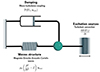 |
Fig. 1. Analogy between the forced and damped mass-spring system, and the inhomogeneous wave equation. |
2.1.3. Source terms
The source term 𝒮 accounts for the forcing of waves by turbulent fields. We can break it into several components to identify the various origins of the energy injection into the modes,
 (15)
(15)
where 𝒮R is the Reynolds-stresses source term,
 (16)
(16)
and 𝒮S is an entropy fluctuations source term,
![Mathematical equation: $$ \begin{aligned} \frac{\partial \mathcal{S} _S}{\partial t} =&- \boldsymbol{\nabla } \cdot (\rho \boldsymbol{U}_t)\boldsymbol{g}_0 - \boldsymbol{\nabla } \left\{ \alpha _s \frac{d \delta s_t}{dt} - \alpha _s \left(\boldsymbol{\boldsymbol{U}_t}\cdot \boldsymbol{\nabla }\right) s_t - \alpha _s \left(\boldsymbol{\boldsymbol{U}_t}\cdot \boldsymbol{\nabla }\right) s_0\right. \nonumber \\&\left.-\boldsymbol{\nabla } \cdot (\rho \boldsymbol{U}_t) \left[c_s^2 + 2 \alpha _{\rho \rho } \rho _t + \alpha _{\rho s} s_t \right] + \left(2 \alpha _{ss} s_t + \alpha _{\rho s} \rho _t \right) \frac{\partial s_t}{\partial t} \right\} . \end{aligned} $$](/articles/aa/full_html/2024/10/aa50802-24/aa50802-24-eq22.gif) (17)
(17)
It was shown recently (Samadi et al. 2015) that this entropy source accounts for less than 10 % of the total power injected into the modes. It is then negligible in solar-like stars in a first step.
𝒮B is the source term due to the magnetic field, that is the turbulent Maxwell stresses,
 (18)
(18)
where δij is the Kronecker symbol, and we used the Einstein summation convention for the tensorial form of the stresses.
2.2. Linear wave operator
The linear wave operator ℒ is decomposed as
 (19)
(19)
where ℒp corresponds to the acoustic character of the waves,
 (20)
(20)
ℒg accounts for the gravity-wave behaviour,
 (21)
(21)
and ℒb is the Alfvén part of the waves,
![Mathematical equation: $$ \begin{aligned} \mathcal{L} _B (\boldsymbol{u}_{\rm osc}, \boldsymbol{b_{\rm osc}})&= \frac{1}{\mu _0}\Bigg [ \bigg (\boldsymbol{\nabla } \cdot {\boldsymbol{\boldsymbol{u}_{\rm osc}}} \bigg ) \bar{\boldsymbol{B}} \times \bigg (\boldsymbol{\nabla } \times {\bar{\boldsymbol{B}}} \bigg ) -\left(\boldsymbol{\bar{\boldsymbol{B}}}\cdot \boldsymbol{\nabla }\right) \boldsymbol{u}_{\rm osc}\nonumber \\&\qquad \times \bigg (\boldsymbol{\nabla } \times {\bar{\boldsymbol{B}}} \bigg ) + \left(\boldsymbol{\boldsymbol{u}_{\rm osc}}\cdot \boldsymbol{\nabla }\right) \bar{\boldsymbol{B}} \times \bigg ( \boldsymbol{\nabla } \times {\bar{\boldsymbol{B}}} \bigg ) \nonumber \\&\qquad + \bar{\boldsymbol{B}} \times \boldsymbol{\nabla } \times {\bigg ( (\boldsymbol{\nabla } \cdot {\boldsymbol{u}_{\rm osc}}) \bar{\boldsymbol{B}} \bigg )} - \bar{\boldsymbol{B}} \times \boldsymbol{\nabla } \times {\bigg ( \left(\boldsymbol{\bar{\boldsymbol{B}}}\cdot \boldsymbol{\nabla }\right) \boldsymbol{u}_{\rm osc} \bigg )}\nonumber \\&\qquad + \bar{\boldsymbol{B}} \times \boldsymbol{\nabla } \times {\bigg (\left(\boldsymbol{\boldsymbol{u}_{\rm osc}}\cdot \boldsymbol{\nabla }\right) \bar{\boldsymbol{B}} \bigg )} - \eta _B \boldsymbol{b_{\rm osc}} \times \boldsymbol{\nabla } \times {\bigg (\Delta \bar{\boldsymbol{B}} \bigg )} \Bigg ]. \end{aligned} $$](/articles/aa/full_html/2024/10/aa50802-24/aa50802-24-eq27.gif) (22)
(22)
The oscillation velocity uosc is coupled to the oscillation magnetic field bosc via the linearised induction equation.
2.2.1. Damping
The damping term can be written as
 (23)
(23)
The term 𝒟0 is due to the non-magnetic part of the inhomogeneous wave equation, which can be recovered as in previous works such as Samadi (2012), Belkacem et al. (2008),
![Mathematical equation: $$ \begin{aligned} \mathcal{D} _0(\boldsymbol{u}_{\rm osc}, \boldsymbol{U}_t)&= \frac{\partial ^2}{\partial t^2} (\rho _t \boldsymbol{u}_{\rm osc}) - \mathcal{L} _0 (\rho _t \boldsymbol{u}_{\rm osc}) + 2 \frac{\partial }{\partial t} \left(\nabla \text{:} \rho \boldsymbol{u}_{\rm osc}\boldsymbol{U}_t \right) \nonumber \\&\quad + \nabla \bigg [ -(2 \alpha _{\rho \rho } \rho _t + \alpha _{\rho s}s_t ) \left(\nabla \cdot (\rho _t \boldsymbol{u}_{\rm osc}) \right) \nonumber \\&\quad - \nabla \cdot (\alpha _s s_t \boldsymbol{u}_{\rm osc}) + \alpha _s (\boldsymbol{u}_{\rm osc}\cdot \nabla ) s_t + s_t (\boldsymbol{u}_{\rm osc}\cdot \nabla ) \alpha _s \bigg ], \end{aligned} $$](/articles/aa/full_html/2024/10/aa50802-24/aa50802-24-eq29.gif) (24)
(24)
where ℒ0 = ℒp + ℒg. 𝒟B is the magnetic contribution to the damping,
 (25)
(25)
2.2.2. Negligible source terms
The term  contains all source terms that are negligible,
![Mathematical equation: $$ \begin{aligned} \frac{\partial \mathcal{C} }{\partial t}&= \frac{( \boldsymbol{\nabla } \times {\bar{B}}) \times \boldsymbol{B_t}}{\mu _0} + \frac{( \boldsymbol{\nabla } \times {\boldsymbol{B_t}}) \times \bar{B}}{\mu _0}\nonumber \\&\qquad + \mathcal{L} (\rho \boldsymbol{U}_t) - \frac{\partial ^2}{\partial t} (\rho \boldsymbol{U}_t) - \frac{\partial }{\partial t} \left( \nabla \text{:} \rho _t \boldsymbol{U}_t \boldsymbol{U}_t \right) + \nonumber \\&\qquad \nabla \left[ -(2 \alpha _{\rho \rho } + \alpha _{\rho s} s_t) \boldsymbol{\nabla } \cdot (\rho \boldsymbol{U}_t) - (2 \alpha _{ss}s_t + 2 \alpha _{\rho s} \rho _t) \frac{\partial s_t}{\partial t} \right.\nonumber \\&\qquad \quad \left. - \alpha _s \boldsymbol{U}_t \cdot \nabla s_t \right]. \end{aligned} $$](/articles/aa/full_html/2024/10/aa50802-24/aa50802-24-eq32.gif) (26)
(26)
It contains linear source terms in turbulent quantities, which do not contribute to the excitation, as well as terms that are negligible due to their order of magnitude (see e.g. Samadi & Goupil 2001, for more details).
2.3. Mode amplitudes
We seek the mean square amplitude of uosc for each mode of a given radial, angular, and azimuthal order (n, ℓ, andm, respectively). The wave Eulerian displacement is written in complex notations as the product between an instantaneous amplitude A(t) and a Lagrangian eigendisplacement ξ(r), which only depends on the position (Samadi & Goupil 2001; Belkacem et al. 2009),
 (27)
(27)
We introduce ω0, the eigenmode frequency, and c. c. denotes the complex conjugate. Deriving Eq. (27) with respect to time leads to the wave velocity,
 (28)
(28)
where we considered that A(t) evolves on a longer timescale than the wave oscillation period. Using Eqs. (14) and (28), we derive the mean squared amplitude of the oscillations,
 (29)
(29)
Subscripts 1 and 2 make reference to spatio-temporal positions  and
and  , respectively. ⟨.⟩ denotes a statistical average performed on an infinite number of independent realisations. We introduce ηD as damping and I as the mode inertia,
 (30)
(30)
where dm is the mass of an elementary fluid parcel. Furthermore, we assumed that turbulence is stationary and homogeneous so that the source term 𝒮 is invariant by any time translation. Although turbulence in magnetohydrodynamics is known to be anisotropic, this assumption is justified by the fact that most of the excitation is due to small-scale eddies (see e.g. Samadi & Goupil 2001).
There are several contributions to the excitation power: 𝒮R2 and 𝒮B2 correspond to the power injected by the Reynolds and Maxwell stresses, respectively. A cross-term also emerges with the combinations in 𝒮B𝒮R.
Figure 2 illustrates the complex interdependences between magnetic field and mode amplitudes: Not only does the magnetic field add up a source term compared with the non-magnetised case, it also indirectly influences the existing source terms, as we list below.
-
The stellar structure is modified by the magnetic force (see e.g. Duez et al. 2010). The stellar density and thermodynamic quantity profiles change, as do the mode frequencies. This is the so-called indirect effect on stellar oscillations (Gough & Thompson 1990).
-
Waves are affected by the magnetic field so that they become magneto-acoustic gravity waves. This changes both the mode frequencies ω0, which are shifted, and the eigenfunctions of the displacement ξ. This is the direct magnetic effect on stellar oscillations (Gough & Thompson 1990).
-
The characteristics of convection strongly affect the source terms. This happens through a change in the mean parameters from MLT such as the convective wavenumber k0 and the convective velocity v0. The magnetic field tends to modify convection by changing the instability threshold (Chandrasekhar 1961). The magnetic field also affects turbulent convection through a change in the kinetic energy spectrum and in the magnetic energy spectrum. (e.g. Brun 2004). This effect of the magnetic field on convection is paramount in our model and is discussed in detail in Section 4.
This complex interplay between the magnetic field and excitation has not been studied in the literature. To give a first overview of the impact of magnetic fields on the stochastic excitation of modes, we use as a first step scaling laws for the modulation of the mode amplitudes as a function of the strength of the magnetic field. These scalings prescriptions could be directly compared to observations. We first adopt a Mixing Length Theory approach to model convection.
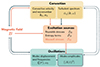 |
Fig. 2. Influence of the magnetic field on the mode amplitudes: Different phenomena. The red arrows represent the effect we take into account. |
3. Scaling laws for the power injected into the modes
To give a very first overview of the impact of magnetism on the stochastic excitation of waves, we use scaling laws to evaluate the mode amplitudes. No physical model includes the effects of magnetic fields so far. The scaling relations have proven to give relevant tendencies and are often used in the litterature, for example in dynamo theories (e.g. Augustson et al. 2019). The energy provided by the stochastic excitation in p-modes is mostly injected very locally at a radius ri in the photosphere (e.g. Samadi & Goupil 2001). As gravity modes are evanescent in the convective zone, they are mostly excited at the base of the convective zone. Under this assumption, Eq. (29) reads
 (31)
(31)
where δ is the usual Dirac function.
We neglected in our model the influence of the magnetic field on the eigenfunctions ξ, which means that ω0 ≫ ωA, where ωA is the Alfvén pulsation. Under this hypothesis, we can use estimates of the source 𝒮 and the damping ηD at the location ri to evaluate the resulting amplitudes of the acoustic modes. For a given mode,
 (32)
(32)
3.1. Scaling of the source terms
First, we estimated the scaling relation of the source terms. As the entropy source term 𝒮s is negligible, we only considered the Reynolds-stresses 𝒮R and the Maxwell-stress 𝒮B source terms.
We introduced ℓosc, which is the typical length of the oscillations. By integrating by part Eq. (29), all the spatial gradients of the source terms Eqs. (16) and (18) can be transferred to the oscillations, as detailed in Samadi & Goupil (2001), Belkacem et al. (2009). Furthermore, the eddies that contribute most to the stochastic excitation are those whose turnover time is near the wave frequency τturnover ∼ ω0. For this reason, we considered that any time derivative amounts to a multiplication by a factor ω0 and any spatial derivative amounts to a multiplication by 1/ℓosc.
We introduce uλ, the velocity of a given convective eddy, with a size λ. We also introduce uc, the MLT convective velocity, which is the velocity of the largest eddy of the turbulent cascade, which has a size Λ. Similarly, bλ is the magnetic field associated with a given eddy with a size λ, while B0 is the magnetic field associated with the largest eddy with a size Λ.
In this framework, the Reynolds-stresses source term scales like
 (33)
(33)
and the Maxwell-stresses source term scales like
 (34)
(34)
Furthermore, scaling relations are often used in turbulence to link uλ and uc. For a given slope α for the kinetic energy spectrum (see e.g. Chapter 1 of Tennekes & Lumley 1972),
 (35)
(35)
The same can be applied to the magnetic cascade,
 (36)
(36)
In Eqs. (35)–(36), we assumed that the magnetic energy spectrum and the kinetic energy spectrum have the same slope α. This is the case for an Iroshnikov-Kraichman spectrum in magnetohydrodynamic turbulence, for which the slope is α = −3/2 for both the kinetic and the magnetic energy spectrum (Iroshnikov 1964; Kraichnan 1965). Depending on the turbulent regimes in magnetohydrodynamics, different values can be found for these spectra, as seen in experiments and direct numerical simulations (see e.g. Sommeria 1986; Biskamp & Müller 2000; Mininni & Pouquet 2009). Finally, when we use Equations (33)–(36) when we take the magnetic fields into account, the resulting source 𝒮mag = 𝒮B + 𝒮R scales like
 (37)
(37)
where we introduced the Alfvén velocity,
 (38)
(38)
As highlighted in Fig. 2, a magnetic field also has an indirect effect on the stochastic excitation as it influences convection. The convective velocity uc must then be evaluated in the framework of magnetised convection and is then expected to be potentially weaker than in non-magnetised convection.
3.2. Scaling of the damping rate
As shown in Eq. (29), it is paramount to know the damping coefficient ηD when the mean mode amplitudes are to be assessed (see Fig. 1). This coefficient is proportional to the loss of energy of the wave. We considered in a first step that damping comes from two phenomena: a turbulent viscous dissipation of the wave, and its Ohmic dissipation. The convective zone of solar-like stars is known to be a turbulent medium. The molecular viscosity is then negligible in front of the turbulent eddy viscosity: ν ∼ νturb. However, more complex formalisms have emerged that take the non-adiabatic fluctuations of density, entropy, and turbulent pressure inside the star into account (e.g. Grigahcène et al. 2005; Belkacem et al. 2012). To compare hydrodynamical and magnetic effects, we restricted ourselves as a first step to the simplest eddy viscosity and Ohmic diffusivity modelling.
The volume loss of energy due to a turbulent viscous dissipation for the wave is
 (39)
(39)
where νt is the eddy viscosity. The turbulent viscosity scales like
 (40)
(40)
where ℓc is the convective characteristic length in MLT.
The volume loss of energy due to Ohmic dissipation for the wave is
 (41)
(41)
where josc is the current density associated with the wave, μ0 is the vacuum magnetic permeability, and ηB is the magnetic diffusivity.
Using the same notations and method as in Section 3.1, we find that
 (42)
(42)
We used the induction Equation (3) but neglected the diffusive term to relate the magnetic field bosc of the wave and the large-scale equilibrium magnetic field  . We find that
 (43)
(43)
Furthermore,
 (44)
(44)
As  from Maxwell-Ampere equation, we derived the scaling relationship for the Ohmic dissipation,
 (45)
(45)
Moreover, we considered that the magnetic field at the injection scale in the turbulent cascade comes from the large-scale magnetic field, such that
 (46)
(46)
The characteristic oscillation length can be expressed with the dispersion relation for acoustic waves,
 (47)
(47)
where cs is the local sound speed. When magnetism is taken into account, the resulting damping contribution is 𝒟mag = 𝒟ohm + 𝒟vis. We have
 (48)
(48)
where 𝒫m ≡ ν/ηB is the magnetic Prandtl number, and ℳ ≡ uc/cs is the local Mach number. We introduced the dimensionless inverse Alfvén number, which corresponds to the ratio of the magnetic and convective kinetic energy,
 (49)
(49)
Again, the convective velocity uc depends on the strength of the magnetic field. To assess the amplitudes of the mean modes appropriately, a proper modelling of magnetised convection is required.
4. Magnetised convection
4.1. Modelling magnetised convection
Magnetic fields modify convection, and connection in turn impacts the excitation sources and damping. The impact of rotation and magnetic fields on convection is of great interest for stellar and planetary evolution (see e.g. Maeder 2009). The most realistic approach to modelling stellar and planetary convective zone is to solve the underlying equations numerically (e.g. Brown et al. 2011; Brun & Browning 2017; Brun et al. 2022).
The available computational resources are finite, however, and therefore, a local model of convection is often used, in particular, for stellar structure modelling and secular evolution. The pioneering studies by Chandrasekhar (1961) and Canuto & Mazzitelli (1991) showed that rotation alone and magnetic fields alone tend to inhibit the convection strength. However, when rotation and magnetic field act together, they tend to destabilise convection with respect to the case of a magnetised but non-rotating fluid or a rotating but non-magnetised fluid (Horn & Aurnou 2022). The interplay between these two phenomena is complex. In this first work, we focus on the case of the magnetic field acting alone. There are two main theoretical approaches to account for the impact of magnetic fields on convection: the instability criterion approach, and the MLT approach.
4.1.1. Instability criterion.
It is key to know under which conditions a star is unstable to convection. Schwarzschild (1906) and Ledoux (1947) derived instability criteria for convection to start, which are used in stellar models. As explained before, convection is stabilised by magnetic fields. At some point, if the external magnetic field is too strong, the fluid becomes stable to convection: We consider that convection is frozen in this case (Gough & Tayler 1966). The value of the minimum magnetic field that freezes convection is the critical magnetic field Bcrit. This approach is an on-off approach to magnetoconvection: Either the external magnetic field B is below Bcrit and convection is active, or B > Bcrit, and there is no more convection (see the illustration Fig. 3a). This is often used in stellar physics to study strongly magnetised stars (see e.g. Jermyn & Cantiello 2020).
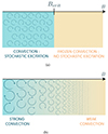 |
Fig. 3. Treatment of the impact of magnetic field on convection, with the critical magnetic field (a), and the Magnetic Mixing- Length Theory (b). |
4.1.2. Mixing-Length Theory
It is quite complex to model turbulent convection because the number of space- and timescales is large. MLT (Böhm-Vitense 1958; Gough 1977) models convection with a single length and velocity scale that corresponds to the characteristics of the most energetic convective eddy. Currently, MLT is implemented in 1D stellar evolution codes to provide the main properties of stellar convection zones.
The critical magnetic field approach described in the previous section does not account for the progressive diminution of the convection strength when an external magnetic field increases. When the magnetic field increases, the turbulent eddies become ever smaller, and their characteristic velocity diminishes. Stevenson (1979) derived a prescription accounting for the modification of MLT by an external magnetic field, rendering the progressive reduction of the convection strength (see Fig. 3b).
In the following subsections, we discuss the theory behind those two approaches and their impact on the stochastic excitation of acoustic modes.
4.2. Critical magnetic field
In non-magnetised fluids, Schwarzschild (1906) derived an instability criterion for convection to begin,
 (50)
(50)
where the temperature gradient is
 (51)
(51)
and the adiabatic temperature gradient is
 (52)
(52)
To take the effects of magnetic fields into account, Gough & Tayler (1966) extended the previous criterion considering an ideal gas with a vertical magnetic field. They showed that convection exists when
 (53)
(53)
where
 (54)
(54)
VA is the Alfvén velocity introduced previously, and cs is the sound speed. The Schwarzschild (Eq. 50) and Gough & Tayler (Eq. 53) criteria make use of the energy principle of Bernstein (1958): They study the change of potential energy δW of any fluid element under a weak perturbation. Necessary and sufficient conditions for stability are obtained by minimising δW with respect to all the possible perturbations. The critical magnetic field above which convection is suppressed can then be assessed,
 (55)
(55)
Gough & Tayler (1966)’s work has been pursued by Newcomb (1961), who showed that a horizontal magnetic field does not influence convection. Moreno-Insertis & Spruit (1989), MacDonald & Mullan (2009), and MacDonald & Petit (2019) generalised the Gough-Tayler criterion to take molecular mass variations μ, non-ideal gas behavior, and radiation pressure into account. For simplicity, we use Eq. (53) derived by Gough & Tayler (1966) in the following. In this framework, the critical inverse Alfvén number above which convection stops is
 (56)
(56)
Once again, as shown in Fig. 3, the critical magnetic field approach fails to account for the progressive variations in the convective velocity uc. To model the stochastic excitation of the modes as seen in Section 3 more precisely, we need a more precise approach to magnetised convection. Here, we considered the Magnetic Mixing-Length Theory, as proposed by Stevenson (1979).
4.3. Magnetic mixing-length theory
Using a linear stability analysis of the convective instability, Stevenson (1979) derived scaling laws for the way in which the convective characteristic velocity and the convective characteristic wavenumber are modified by magnetic fields. This study was made under the hypothesis that the dominant convective mode carries the highest energy (Malkus & Chandrasekhar 1997). Stevenson (1979) derived a modulation factor in each case: the convective velocity (convective wavenumber) with magnetism uc (kc) is expressed with respect to the convective velocity (convective wavenumber) without magnetism u0 (k0),
 (57)
(57)
Stevenson (1979) derived scalings for the functions  and
and  for the asymptotic limits A ≪ 1 (low magnetic field) and A ≫ 1 (strong magnetic field). His prescriptions are detailed in Table 1. These scaling laws are illustrated in Fig. 4 for regimes with weak and strong magnetic fields. As expected, the convective velocity decreases when the magnetic field increases: the magnetic field has a stabilising effect on convection. Moreover, the convective wavenumber rises when the magnetic field is stronger. The size of the dominant eddy in the MLT framework then diminishes, as previously illustrated in Fig. 4.
Values of the modulation factors  and
and  (Stevenson 1979).
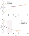 |
Fig. 4. Scaling laws given by Stevenson for the change in (top) wavenumber |


Stevenson (1979) also provided prescriptions for rotating convection and set the ground for the rotating mixing-length theory (hereafter R-MLT). This method was extended by adding the impact of diffusive processes in rotating convection (Augustson & Mathis 2019). In the regime of low convective Rossby numbers, the Stevenson (1979) scalings appear to hold well when compared to direct numerical simulations of rotating convection (Barker et al. 2014; Vasil et al. 2021; Korre & Featherstone 2021), with interesting results for the internal structure of low-mass and massive stars and for the mixing in the evolution of giant planets (Michielsen et al. 2019; Dumont et al. 2021; Fuentes et al. 2022). Despite some numerical simulations of magnetised convection (e.g. Hotta 2018), no direct comparison of Stevenson’s prescriptions for M-MLT has been made so far. Because the physical approach for the rotating and magnetic case is identical, we can expect that the prediction for the Magnetic Mixing Length Theory are reliable.
One way of confirming Stevenson’s prescription in M-MLT is to compare it with the critical magnetic field approach detailed in 4.2. To do this, we used the stellar structure and evolution code MESA (Paxton et al. 2011, 2013, 2015, 2018, 2019; Jermyn et al. 2023) to generate a 1D stellar model of the Sun (see Appendix A for the inlist we used). At the top of the convective zone, we find a maximum Acrit ∼ 103, with Gough & Tayler (1966) stability criterion (Eq. 56). According to Stevenson’s prescriptions, the convective velocity has diminished by 97% at this point: We can therefore consider that convection is very weak compared to the non-magnetised case. The comparison is illustrated in Fig. 5. At first glance, Stevenson (1979)’scalings are thus consistent with the widespread critical magnetic field approach. It is an adequate prescription for the stochastic excitation of stellar oscillations in the presence of magnetism.
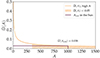 |
Fig. 5. Critical A parameter in the Sun compared with Stevenson’ scaling laws. In the orange zone, the convective velocity has diminished by more than 95% with respect to the non-magnetised case. The purple line represents the position of the critical magnetic field in the Sun. |
5. Influence of magnetised convection on the resulting amplitude
5.1. Modification of the source and of the damping in magnetised convection
Using the Stevenson (1979) prescription of magnetised convection detailed in the previous section, we accounted for the modification of convection by magnetism for the driving and the damping of the oscillations. Without magnetic fields, the driving of the excitation is reduced to the Reynolds-stresses source term in non-magnetised convection. We denote with 𝒮0 the dominant excitation source without magnetism,
 (58)
(58)
For reference, the symbols that are frequently used from this section are listed in Table 2. The magnetic field influences the stochastic excitation at different levels:
-
The magnetic Maxwell-stresses 𝒮B also contribute to the excitation, along with the Reynolds stress 𝒮R.
-
The convective velocity is modified by the magnetic field in the Maxwell stress 𝒮B and in the Reynolds stress source term 𝒮R.
When we used M-MLT with the expressions of Table 1, we found that the resulting source term with magnetic fields was modulated by a function  when compared to the non-magnetised source term,
 (59)
(59)
Frequently used symbols in the stochastic excitation model.
The modulation of the source term  is plotted in Fig. 6, following the M-MLT scalings of Stevenson (1979) in Table 1. In the low A regime (10−5 < A < 10−2, the magnetic field does not significantly lower the driving of the oscillations. From A ∼ 10−2 to A ∼ 1, the source term is diminished when the magnetic field is stronger: convection becomes lower due to the magnetic field. In the high A regime (A > 1), the Maxwell stresses become the dominant excitation source:
  rises when A increases.
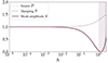 |
Fig. 6. Scaling as a function of the inverse Alfvén number A. |
Similarly, the damping terms are also modified because of the Ohmic diffusion and of the modification of the eddy viscosity since convective velocities and length scales that intervene in its definition (Eq. 40) are impacted by magnetic fields. We obtain
 (60)
(60)
where 𝒟0 is the damping without a magnetic field, and  is the modulation factor when the influence of a magnetic field is added. We note that the damping does not affect all the acoustic modes equally: it depends on the mode velocity uosc. To give a trend of how damping is affected by magnetic fields, we considered a turbulent region where νt ∼ ηB, leading to 𝒫m = 1. In the Sun, the Mach number ℳ reaches a maximum of ℳ ∼ 0.3 at the top of the convective zone. It then leads to an upper limit for the damping. Under this simplification, the asymptotic expressions are detailed in Table 3, again making use of the Stevenson (1979) asymptotic scalings in M-MLT. The damping of the oscillations slightly increases until A ∼ 1: The Ohmic damping increases when the magnetic field is stronger. However, the damping saturates in the high A regime (A > 1). In this regime, the convection increasingly diminishes with the increase in the magnetic field, so that the viscous damping decreases, which compensates for the increase in the Ohmic turbulent damping.
Modulation of the source term of the oscillations ( ) and the damping (
 ) in the asymptotic limits A ≪ 1 and A ≫ 1.
5.2. Mean squared amplitude with a magnetic field
When we know how the driving and the damping of the oscillations are affected by the magnetic field, we can give a tendency for the modification of the resulting mode amplitudes. Following Eq. (31), we introduce ⟨|A(t)|2⟩mag, the mean mode amplitude in the magnetised case, and ⟨|A(t)|2⟩0, the mean amplitude in the non-magnetised case. As in the previous subsection,  accounts for the modulation of the mean mode amplitude by magnetic fields. Again with Eq. (31), we have
 (61)
(61)
Fig. 6 shows the resulting modulations of the mode amplitudes. Because of the distinct asymptotic regimes of magnetised convection in Stevenson (1979), there is a discontinuity at A = 1, 28. In this model, the damping slightly influences the modulation of the mode amplitude, but the overall tendency is dominated by the variations in the source terms  . For low values of A, and more strongly between A = 10−1 and A = 1/2, the magnetic field tends to inhibit the source of the stochastic excitation. Under A = 10−4, there is nearly no change because the Maxwell stress source term is too low. For higher values of A, there is an increase in the excitation. As 𝒮B/𝒮R ∼ A/2, so for A > 2, the Maxwell stresses become higher than the Reynolds stresses, and the magnetic source term dominates the stochastic excitation.
This tendency qualitatively agrees with the observations of Garcia et al. (2010). These authors showed that the p-mode amplitudes were modulated during the magnetic cycle of a Sun-like star, HD49933. They used the frequency shifts induced by the magnetic field to assess the magnetic activity of the star. They observed that the stronger the magnetic field, the lower the mode amplitudes (and vice versa). This is the tendency we predict as well, using these scaling laws.
The Sun’s large-scale magnetic field at the surface is Bsurf ∼ 4G − 8G, depending on the moment of the magnetic cycle. It corresponds to an inverse Alfvén number between A = 7 ⋅ 10−4 and A = 1 ⋅ 10−3: In this range,  is close to one, so that the magnetic field slightly inhibits the excitation source, but no significant change is expected.
6. Conclusion and perspectives
We shed light on the stochastic excitation of stellar oscillations when a magnetic field is present. We drew a first picture of the power injected into the modes considering both the magnetic source term that emerges, the Maxwell stress source term, and the modification of convection by the magnetic field. After generalising the forced wave equation with a magnetic field, we provided scaling laws for the excitation source and the damping, making use of Stevenson (1979)’s prescriptions in the simplified framework of the magnetic mixing-length theory. Moreover, we used a 1D solar model to show that Stevenson’s prescriptions for magnetised convection agree well with the existing theory of a critical magnetic field above which convection is frozen. We then demonstrated that the mode amplitudes tend to decrease with the magnetic field intensity for p-modes. This might explain the observations in García & Ballot (2019) where some mode amplitudes variations were detected following a magnetic cycle: the lower the magnetic activity, the higher the mode amplitudes, and vice versa. Therefore, it could explain why p-modes are not detected in stars with a high level of magnetic activity, as has been observed for solar-type stars observed by the Kepler mission (Mathur et al. 2019). These scaling laws should be compared with the observations of the full Kepler sample: An approach combining both 1D stellar evolution modelling to access the inverse Alfvén number parameter and observational data of p-modes will be relevant. The results presented in Mathur et al. (2019) were presented as a function of the stellar rotation period and of the magnetic activity index, Sph. In a near future, it would be important to establish the relation between Sph and the magnetic field B, and in turn, of the inverse Alfvén number A, to compare the data with our theoretical prediction. To proceed with scaling laws, analytical work is ongoing to build on this theoretical formalism and render the contribution of different sources more precisely using a spectral description of magneto-hydrodynamic turbulence. This work will help us to model the stochastic excitation in the presence of magnetic field more precisely.
Our work will be extended and adapted to study the stochastic excitation of gravity waves (Lecoanet & Quataert 2013) as well as magneto-gravito-inertial waves (Mathis & de Brye 2011; Rui & Fuller 2023; Rui et al. 2024). These waves are excited at the base of the convective zone because they are evanescent in the convective zone. Understanding their propagation and excitation is paramount because they are one of the best candidates for the strong angular momentum transport needed in stellar radiative zones to reproduce the observed internal rotation revealed in stars by helio- and asteroseismology (see e.g. Schatzman 1993; Zahn et al. 1997; Rogers et al. 2013). This in turn might yield new insights into the rotational profiles and internal chemical mixing of rotating and magnetic stars.
Finally, the magnetic field generated by the dynamo effect strongly depends on rotation (e.g. Brun & Browning 2017): The combined impact of rotation and the magnetic field on the stochastic excitation of stellar oscillations by turbulent convection must therefore be studied. This would allow us to predict the excitation of waves in both rotating and magnetised stars more accurately.
Acknowledgments
The authors are grateful to the referee for their detailed and constructive report, which has allowed us to improve this article. L.B. and S.M. acknowledge support from the European Research Council (ERC) under the Horizon Europe program (Synergy Grant agreement 101071505: 4D-STAR), from the CNES SOHO-GOLF and PLATO grants at CEA-DAp, and from PNPS (CNRS/INSU). While partially funded by the European Union, views and opinions expressed are however those of the author only and do not necessarily reflect those of the European Union or the European Research Council. Neither the European Union nor the granting authority can be held responsible for them.
References
- Aerts, C. 2021, Rev. Mod. Phys., 93, 015001 [Google Scholar]
- Augustson, K. C., & Mathis, S. 2019, ApJ, 874, 83 [Google Scholar]
- Augustson, K. C., Brown, B. P., Brun, A. S., Miesch, M. S., & Toomre, J. 2012, ApJ, 756, 169 [Google Scholar]
- Augustson, K. C., Brun, A. S., & Toomre, J. 2019, ApJ, 876, 83 [Google Scholar]
- Augustson, K. C., Mathis, S., & Astoul, A. 2020, ApJ, 903, 90 [NASA ADS] [CrossRef] [Google Scholar]
- Balmforth, N. J. 1992a, MNRAS, 255, 639 [NASA ADS] [Google Scholar]
- Balmforth, N. J. 1992b, MNRAS, 255, 632 [NASA ADS] [CrossRef] [Google Scholar]
- Barker, A. J., Dempsey, A. M., & Lithwick, Y. 2014, ApJ, 791, 13 [Google Scholar]
- Belkacem, K., Samadi, R., Goupil, M. J., & Dupret, M. A. 2008, A&A, 478, 163 [NASA ADS] [CrossRef] [EDP Sciences] [Google Scholar]
- Belkacem, K., Mathis, S., Goupil, M. J., & Samadi, R. 2009, A&A, 508, 345 [NASA ADS] [CrossRef] [EDP Sciences] [Google Scholar]
- Belkacem, K., Dupret, M. A., Baudin, F., et al. 2012, A&A, 540, L7 [NASA ADS] [CrossRef] [EDP Sciences] [Google Scholar]
- Bernstein, I. 1958, An Energy Principle for Hydromagnetic Stability Problems (Royal Society) [Google Scholar]
- Biskamp, D., & Müller, W.-C. 2000, Phys. Plasma, 7, 4889 [NASA ADS] [CrossRef] [Google Scholar]
- Böhm-Vitense, E. 1958, Z. Astrophys., 46, 108 [Google Scholar]
- Brown, B. P., Browning, M. K., Brun, A. S., Miesch, M. S., & Toomre, J. 2008, ApJ, 689, 1354 [CrossRef] [Google Scholar]
- Brown, B. P., Miesch, M. S., Browning, M. K., Brun, A. S., & Toomre, J. 2011, ApJ, 731, 69 [Google Scholar]
- Brun, A. S. 2004, Sol. Phys., 220, 333 [NASA ADS] [CrossRef] [Google Scholar]
- Brun, A. S., & Browning, M. K. 2017, Liv. Rev. Sol. Phys., 14, 4 [Google Scholar]
- Brun, A. S., Miesch, M. S., & Toomre, J. 2004, ApJ, 614, 1073 [Google Scholar]
- Brun, A. S., Strugarek, A., Noraz, Q., et al. 2022, ApJ, 926, 21 [NASA ADS] [CrossRef] [Google Scholar]
- Buffett, B., & Knezek, N. 2018, Geophys. J. Int., 212, 1523 [NASA ADS] [CrossRef] [Google Scholar]
- Canuto, V. M., & Mazzitelli, I. 1991, ApJ, 370, 295 [NASA ADS] [CrossRef] [Google Scholar]
- Chandrasekhar, S. 1961, Hydrodynamic and Hydromagnetic Stability (Oxford: Clarendon) [Google Scholar]
- Chaplin, W. J., Bedding, T. R., Bonanno, A., et al. 2011, ApJ, 732, L5 [Google Scholar]
- Charbonneau, P. 2010, Living Rev. Sol. Phys., 7, 3 [NASA ADS] [CrossRef] [Google Scholar]
- Christensen-Dalsgaard, J. 2015, A Bright Outlook for Helio-and Asteroseismology (Cambridge University Press) [Google Scholar]
- Cowling, T. G. 1941, MNRAS, 101, 367 [NASA ADS] [Google Scholar]
- Currie, L. K., Barker, A. J., Lithwick, Y., & Browning, M. K. 2020, MNRAS, 493, 5233 [CrossRef] [Google Scholar]
- Duez, V., Mathis, S., & Turck-Chiéze, S. 2010, MNRAS, 402, 271 [NASA ADS] [CrossRef] [Google Scholar]
- Dumont, T., Palacios, A., Charbonnel, C., et al. 2021, A&A, 646, A48 [EDP Sciences] [Google Scholar]
- Frisch, U. 1995, Turbulence: The Legacy of A. N. Kolmogorov (Cambridge University Press) [Google Scholar]
- Fuentes, J. R., Cumming, A., & Anders, E. H. 2022, Phys. Rev. Fluids, 7, 124501 [NASA ADS] [CrossRef] [Google Scholar]
- García, R. A., & Ballot, J. 2019, Liv. Rev. Sol. Phys., 16, 4 [Google Scholar]
- García, R. A., Turck-Chièze, S., Jiménez-Reyes, S. J., et al. 2007, Science, 316, 1591 [Google Scholar]
- Garcia, R. A., Mathur, S., Salabert, D., et al. 2010, Science, 329, 1032 [NASA ADS] [CrossRef] [Google Scholar]
- Gizon, L., Ballot, J., Michel, E., et al. 2013, PNAS, 110, 13267 [NASA ADS] [CrossRef] [Google Scholar]
- Goldreich, P., & Keeley, D. A. 1977, ApJ, 212, 243 [NASA ADS] [CrossRef] [Google Scholar]
- Goldreich, P., & Kumar, P. 1990, ApJ, 363, 694 [NASA ADS] [CrossRef] [Google Scholar]
- Goldreich, P., & Kumar, P. 1991, ApJ, 374, 366 [NASA ADS] [CrossRef] [Google Scholar]
- Gough, D. O. 1977, ApJ, 214, 196 [NASA ADS] [CrossRef] [Google Scholar]
- Gough, D. O., & Tayler, R. J. 1966, MNRAS, 133, 85 [Google Scholar]
- Gough, D. O., & Thompson, M. J. 1990, MNRAS, 242, 25 [Google Scholar]
- Goupil, M. J., Catala, C., Samadi, R., et al. 2024, A&A, 683, A78 [NASA ADS] [CrossRef] [EDP Sciences] [Google Scholar]
- Grigahcène, A., Dupret, M.-A., Gabriel, M., Garrido, R., & Scuflaire, R. 2005, A&A, 434, 1055 [NASA ADS] [CrossRef] [EDP Sciences] [Google Scholar]
- Horn, S., & Aurnou, J. M. 2022, Proc. R. Soc. A, 478, 20220313 [NASA ADS] [CrossRef] [Google Scholar]
- Hotta, H. 2018, ApJ, 860, L24 [NASA ADS] [CrossRef] [Google Scholar]
- Huber, K. F., Czesla, S., Wolter, U., & Schmitt, J. H. M. M. 2009, A&A, 508, 901 [NASA ADS] [CrossRef] [EDP Sciences] [Google Scholar]
- Iroshnikov, P. S. 1964, Sov. Astron., 7, 566 [NASA ADS] [Google Scholar]
- Jermyn, A. S., & Cantiello, M. 2020, ApJ, 900, 113 [NASA ADS] [CrossRef] [Google Scholar]
- Jermyn, A. S., Bauer, E. B., Schwab, J., et al. 2023, ApJS, 265, 15 [NASA ADS] [CrossRef] [Google Scholar]
- Käpylä, P. J., Korpi, M. J., Stix, M., & Tuominen, I. 2005, A&A, 438, 403 [NASA ADS] [CrossRef] [EDP Sciences] [Google Scholar]
- Kiefer, R., Schad, A., Davies, G., & Roth, M. 2017, A&A, 598, A77 [NASA ADS] [CrossRef] [EDP Sciences] [Google Scholar]
- Korre, L., & Featherstone, N. A. 2021, ApJ, 923, 52 [NASA ADS] [CrossRef] [Google Scholar]
- Kraichnan, R. H. 1965, Phys. Fluids, 8, 1385 [Google Scholar]
- Lecoanet, D., & Quataert, E. 2013, MNRAS, 430, 2363 [Google Scholar]
- Ledoux, P. 1947, ApJ, 105, 305 [NASA ADS] [CrossRef] [Google Scholar]
- Leibacher, J. W., & Stein, R. F. 1971, ApJ, 7, L191 [Google Scholar]
- Lesieur, M. 2008, Fluid Mechanics and its Applications (Springer) [CrossRef] [Google Scholar]
- Lighthill, M. J. 1952, Proc. R. Soc. London, Ser. A, 211, 564 [NASA ADS] [CrossRef] [Google Scholar]
- MacDonald, J., & Mullan, D. J. 2009, ApJ, 700, 387 [Google Scholar]
- MacDonald, J., & Petit, V. 2019, MNRAS, 487, 3904 [NASA ADS] [CrossRef] [Google Scholar]
- Maeder, A. 2009, Astronomy and Astrophysics Library (Berlin, Heidelberg: Springer) [CrossRef] [Google Scholar]
- Malkus, W. V. R., & Chandrasekhar, S. 1997, Proc. R. Soc. London, Ser. A, 225, 196 [Google Scholar]
- Mathis, S. 2009, A&A, 506, 811 [CrossRef] [EDP Sciences] [Google Scholar]
- Mathis, S., & de Brye, N. 2011, A&A, 526, A65 [CrossRef] [EDP Sciences] [Google Scholar]
- Mathur, S., García, R. A., Bugnet, L., et al. 2019, Front. Astron. Space Sci., 6, 17 [NASA ADS] [CrossRef] [Google Scholar]
- Michielsen, M., Pedersen, M. G., Augustson, K. C., Mathis, S., & Aerts, C. 2019, A&A, 628, A76 [NASA ADS] [CrossRef] [EDP Sciences] [Google Scholar]
- Mininni, P. D., & Pouquet, A. 2009, Phys. Rev. E, 80 [CrossRef] [Google Scholar]
- Moreno-Insertis, F., & Spruit, H. C. 1989, ApJ, 342, 1158 [NASA ADS] [CrossRef] [Google Scholar]
- Newcomb, W. A. 1961, The. Phys. Fluids, 4, 391 [NASA ADS] [CrossRef] [Google Scholar]
- Paxton, B., Bildsten, L., Dotter, A., et al. 2011, ApJS, 192, 3 [Google Scholar]
- Paxton, B., Cantiello, M., Arras, P., et al. 2013, ApJS, 208, 4 [Google Scholar]
- Paxton, B., Marchant, P., Schwab, J., et al. 2015, ApJS, 220, 15 [Google Scholar]
- Paxton, B., Schwab, J., Bauer, E. B., et al. 2018, ApJS, 234, 34 [NASA ADS] [CrossRef] [Google Scholar]
- Paxton, B., Smolec, R., Schwab, J., et al. 2019, ApJS, 243, 10 [Google Scholar]
- Philidet, J., Belkacem, K., Samadi, R., Barban, C., & Ludwig, H.-G. 2020, A&A, 635, A81 [NASA ADS] [CrossRef] [EDP Sciences] [Google Scholar]
- Press, W. H. 1981, ApJ, 245, 286 [Google Scholar]
- Rauer, H., Catala, C., Aerts, C., et al. 2014, Exp. Astron., 38, 249 [Google Scholar]
- Rogers, T. M., Lin, D. N. C., McElwaine, J. N., & Lau, H. H. B. 2013, ApJ, 772, 21 [NASA ADS] [CrossRef] [Google Scholar]
- Rui, N. Z., & Fuller, J. 2023, MNRAS, 523, 582 [NASA ADS] [CrossRef] [Google Scholar]
- Rui, N. Z., Ong, J. M. J., & Mathis, S. 2024, MNRAS, 527, 6346 [Google Scholar]
- Salabert, D., Régulo, C., Pérez Hernández, F., & García, R. A. 2018, A&A, 611, A84 [NASA ADS] [CrossRef] [EDP Sciences] [Google Scholar]
- Samadi, R. 2012, Thesis, Université Pierre et Marie Curie– Paris VI [Google Scholar]
- Samadi, R., & Goupil, M.-J. 2001, A&A, 370, 136 [NASA ADS] [CrossRef] [EDP Sciences] [Google Scholar]
- Samadi, R., Belkacem, K., & Sonoi, T. 2015, EAS Pub. Ser., 111, 73 [Google Scholar]
- Santos, A. R. G., Campante, T. L., Chaplin, W. J., et al. 2018, ApJS, 237, 17 [NASA ADS] [CrossRef] [Google Scholar]
- Schatzman, E. 1993, A&A, 279, 431 [NASA ADS] [Google Scholar]
- Schwarzschild, K. 1906, Nachrichten von der Königlichen Gesellschaft der Wissenschaften zu Göttingen, Math.-phys. Klasse, 195, 41 [Google Scholar]
- Sommeria, J. 1986, J. Fluid Mech., 170, 139 [NASA ADS] [CrossRef] [Google Scholar]
- Stein, R. F. 1967, AJ, 72, 321 [NASA ADS] [Google Scholar]
- Stevenson, D. J. 1979, Geophys. Astrophys. Fluid Dyn., 12, 139 [NASA ADS] [CrossRef] [Google Scholar]
- Tennekes, H., & Lumley, J. L. 1972, First Course in Turbulence (Cambridge: MIT Press) [CrossRef] [Google Scholar]
- Thompson, M. J., Christensen-Dalsgaard, J., Miesch, M. S., & Toomre, J. 2003, ARA&A, 41, 599 [Google Scholar]
- Townsend, R. H. D., & Teitler, S. A. 2013, MNRAS, 435, 3406 [Google Scholar]
- Ulrich, R. K. 1970, ApJ, 162, 993 [NASA ADS] [CrossRef] [Google Scholar]
- Vasil, G. M., Julien, K., & Featherstone, N. A. 2021, PNAS, 118, e2022518118 [NASA ADS] [CrossRef] [Google Scholar]
- Zahn, J. P., Talon, S., & Matias, J. 1997, A&A, 322, 320 [NASA ADS] [Google Scholar]
Appendix A: MESA Inlists for the solar model
&kap
 ! kap options
 ! see kap/defaults/kap.defaults
 use_Type2_opacities = .true.
 Zbase = 0.016

 / ! end of kap namelist

&controls

  initial_mass = 1.0
  ! MAIN PARAMS
  mixing_length_alpha = 1.9446893445
  initial_z = 0.02
  do_conv_premix = .true.
  use_Ledoux_criterion = .true.

  ! OUTPUT
  max_num_profile_models = 100000
  profile_interval = 300
  history_interval = 1
  photo_interval = 300

  ! WHEN TO STOP
  xa_central_lower_limit_species(1) = 'h1'
  xa_central_lower_limit(1) = 0.01
  max_age = 6.408d9

  ! RESOLUTION
  mesh_delta_coeff = 0.5
  time_delta_coeff = 1.0

  ! GOLD TOLERANCES
  use_gold_tolerances = .true.
  use_gold2_tolerances = .true.
  delta_lg_XH_cntr_limit = 0.01
  min_timestep_limit = 1d-1

  !limit on magnitude of relative change at any grid point
  delta_lgTeff_limit = 0.25 ! 0.005
  delta_lgTeff_hard_limit = 0.25 ! 0.005
  delta_lgL_limit = 0.25 ! 0.005

  ! asteroseismology
  write_pulse_data_with_profile = .true.
  pulse_data_format = 'FGONG'

  ! add_atmosphere_to_pulse_data = .true.

  ! rename the output directory
  log_directory = 'LOGS_SUN_Z_0.04'


/ ! end of controls namelist

&pgstar


/ ! end of pgstar namelist
All Tables
Modulation of the source term of the oscillations () and the damping () in the asymptotic limits A ≪ 1 and A ≫ 1.
All Figures
|
Fig. 1. Analogy between the forced and damped mass-spring system, and the inhomogeneous wave equation. |
| In the text | |
|
Fig. 2. Influence of the magnetic field on the mode amplitudes: Different phenomena. The red arrows represent the effect we take into account. |
| In the text | |
|
Fig. 3. Treatment of the impact of magnetic field on convection, with the critical magnetic field (a), and the Magnetic Mixing- Length Theory (b). |
| In the text | |
|
Fig. 4. Scaling laws given by Stevenson for the change in (top) wavenumber |
| In the text | |
|
Fig. 5. Critical A parameter in the Sun compared with Stevenson’ scaling laws. In the orange zone, the convective velocity has diminished by more than 95% with respect to the non-magnetised case. The purple line represents the position of the critical magnetic field in the Sun. |
| In the text | |
|
Fig. 6. Scaling as a function of the inverse Alfvén number A. |
| In the text | |
Current usage metrics show cumulative count of Article Views (full-text article views including HTML views, PDF and ePub downloads, according to the available data) and Abstracts Views on Vision4Press platform.
Data correspond to usage on the plateform after 2015. The current usage metrics is available 48-96 hours after online publication and is updated daily on week days.
Initial download of the metrics may take a while.