© F. H. Navarrete et al. 2022

1. Introduction

Eclipsing time variations (ETVs) have been observed in a wide range of post-common-envelope binaries (PCEBs; Zorotovic & Schreiber 2013; Bours et al. 2016). Traditionally, two explanations have been proposed for the observed variations: One explanation refers to the possible presence of a third body, preferentially with a mass of a few Jupiter masses in the case of NN Ser (Beuermann et al. 2010) and a brown dwarf of 0.035 M_⊙ in V471 Tau (Vaccaro et al. 2015), and on a wide orbit, which could explain the observed ETVs as due to the orbit of the binary system around the common center of mass via the light travel time effect (e.g., Beuermann et al. 2012, 2013). The presence of such planets might be explained either because they survived the common-envelope event (Völschow et al. 2014) or because they formed from the ejecta of common-envelope material (Schleicher & Dreizler 2014). However, the planetary systems were sometimes found to be unstable (Mustill et al. 2013), and at other times, the predicted planets were not detected (Hardy et al. 2015).

An alternative possibility is that the ETVs is caused in the binary system itself, as a result of magnetic activity. This might occur in different forms. An early suggestion by Decampli & Baliunas (1979) considered a rocket effect produced by anisotropic mass loss, but the hypothesis was finally rejected. Tidal torques are another possibility, but their magnitudes are so low (Zahn & Bouchet 1989; Ogilvie & Lin 2007) that they cannot transfer the necessary angular momentum (Applegate & Patterson 1987). As a different solution, both Matese & Whitmire (1983) and Applegate & Patterson (1987) proposed that the orbital period would be changed if the stellar quadrupole moment changed as a result of magnetic activity.

This was a central step, but the cause for the change in the stellar quadrupole moment remains to be defined and its strength needs to be determined. In the original models (e.g., Matese & Whitmire 1983; Applegate & Patterson 1987), it was assumed that the magnetic field deforms the star by causing a deviation from its hydrostatic equilibrium, requiring thus a very strong magnetic field. Marsh & Pringle (1990) showed, however, that the required periodic deformation was too strong to be sustained by the luminosity of the star. A different scenario thus emerged in which the change of the quadrupole moment is not caused directly by the magnetic field, but is a result of angular momentum redistribution inside the star through the dynamo process, which then leads to stellar distortions as a result of the centrifugal force (Applegate 1992). Within a simplified thin-shell model, considering an inner core and an infinitely thin shell, Applegate (1992) calculated the quadrupole moment of the shell as

$$\begin{array}{c}\hfill Q=\frac{1}{9}{M}_s{R}^2\left(\frac{{\mathrm{\Omega }}^2{R}^3}{\mathit{GM}}\right),\end{array}$$(1)

where M is the mass of the star, M_s ≪ M is the mass of the shell, Ω is the angular velocity of the shell, R is the radius from the center of the star to the shell, and G is the gravitational constant. Applegate (1992) calculated the angular momentum to be transferred within the star to produce a period variation ΔP as

$$\begin{array}{c}\hfill \mathrm{\Delta }J=-\frac{G{M}^2}{R}{\left(\frac{a}{R}\right)}^2\frac{\mathrm{\Delta }P}{6\pi },\end{array}$$(2)

with a the separation of the binary system. The energy required to transfer the angular momentum is then

$$\begin{array}{c}\hfill \mathrm{\Delta }E={\mathrm{\Omega }}_{\mathit{dr}}\mathrm{\Delta }J+\frac{{(\mathrm{\Delta }J)}^2}{2I_{\mathrm{eff}}},\end{array}$$(3)

where Ω_dr refers to the difference of angular velocity between the shell and the core, and I_eff is the effective moment of inertia, corresponding to about half of the inertial moment of the shell.

This model was extended by Brinkworth et al. (2006), who considered a finite instead of an infinitely thin shell, showing that the latter increased the energy required to produce the deformation by roughly one order of magnitude. Völschow et al. (2016) subsequently applied this model in a systematic way to the sample of Zorotovic & Schreiber (2013), showing that the energy requirement is sometimes fulfilled and sometimes it is not. A similar conclusion was obtained by Navarrete et al. (2018) through an extension of the analysis. On the other hand, more detailed 1D models solving the evolution equation for the stellar angular momentum indicated that the energetic requirement may actually be reduced (Lanza 2006), and Völschow et al. (2018) concluded that the mechanism is feasible for stars with masses of 0.3 − 0.36 M_⊙.

Other types of solutions have also been proposed. For instance, Applegate (1989) derived librating and circulating solutions in the presence of a constant quadrupole moment, although they were originally predicted to provide modulations over shorter periods than observed in the PCEBs. Lanza (2020) re-examined this scenario, however, and proposed that a persistent nonaxisymmetric internal magnetic field could produce an appropriate quadrupole moment to explain the observed deviations at a much lower energetic expense than in the scenario in which the quadrupole moment variation is produced via the centrifugal force (e.g., Applegate 1992).

This problem was recently revisited in 3D magnetohydrodynamical (MHD) simulations, and although the centrifugal force was not included, quasi-periodic quadrupole moment variations caused by magnetic activity were found. They were roughly still one order of magnitude lower than required by observations, however (Navarrete et al. 2020). As they were not driven via the centrifugal force, it seems more likely that a change in the internal circulation in the star rather than a redistribution of the angular momentum has caused this result. This was recently confirmed via an extended set of simulations with a more detailed analysis (Navarrete et al. 2022).

As the correct mechanism that gives rise to the ETVs is still not established, it is fundamental to investigate how the centrifugal force influences the change in the quadrupole moment within the stars. For this purpose, we present 3D MHD simulations of a solar-mass star that include and vary the centrifugal force to assess in this way how it affects the stellar structure. Thus, we aim to verify whether the origin of these variations is based on the centrifugal force as proposed by Applegate (1992), or if other mechanisms must be at play to cause the observed variations. Our numerical approach is presented in Sect. 2, and the results are given in Sect. 3. We finally present our discussion and conclusions in Sect. 4.

2. Model

We present two sets of simulations with rotation rates 20Ω_⊙ and 30Ω_⊙, where Ω_⊙ is the solar rotation rate. These are part of an overall larger set of simulations that has been pursued to analyze dynamos in the context of young stars (Navarrete et al., in prep.). We label the first set simulation group C and the second set group D. Within each set, we varied the centrifugal force amplitude.

The compressible MHD equations were solved on a spherical grid with coordinates (r, θ, ϕ), where 0.7 ≤ r ≤ R is the radial coordinate, R is the radius of the star, π/12 ≤ θ ≤ 11π/12 is the colatitude, and 0 ≤ ϕ < 2π is the longitude. The model is the same as in Käpylä et al. (2013) and Navarrete et al. (2020, 2022). The equations were solved in the following form:

$$\begin{array}{cc}\hfill \frac{\partial \mathit{A}}{\partial t}& =\mathit{u}\times \mathit{B}-\eta {\mu }_0\mathit{J},\hfill \end{array}$$(4)

$$\begin{array}{cc}\hfill \frac{\mathrm{D}ln\rho }{\mathrm{D}t}& =-\mathbf{\nabla }\mathbf{·}\mathit{u},\hfill \end{array}$$(5)

$$\begin{array}{cc}\hfill \frac{\mathrm{D}\mathit{u}}{\mathrm{D}t}& ={\mathcal{F}}^{\mathrm{grav}}+{\mathcal{F}}^{\mathrm{Cor}}+{\mathcal{F}}^{\mathrm{cent}}-\frac{1}{\rho }(\mathbf{\nabla }p-\mathit{J}\times \mathit{B}-\mathbf{\nabla }\mathbf{·}2\nu \rho \mathit{S}),\hfill \end{array}$$(6)

$$\begin{array}{cc}\hfill T\frac{\mathrm{D}s}{\mathrm{D}t}& =\frac{1}{\rho }[\eta {\mu }_0{\mathit{J}}^2-\mathbf{\nabla }\mathbf{·}({\mathit{F}}^{\mathrm{rad}}+{\mathit{F}}^{\mathrm{SGS}})]+2\nu {\mathit{S}}^2,\hfill \end{array}$$(7)

where A is the magnetic vector potential, B = ∇ × A is the magnetic field, u is the velocity field, η is the magnetic diffusivity, μ₀ is the vacuum permittivity, J is the current density, ρ is the density, p is the pressure, ν is the viscosity, S is the rate of strain tensor, T is the temperature, and s is the entropy. F^rad and F^SGS are the radiative and the subgrid scale fluxes, respectively (see, e.g., Käpylä et al. 2013). The SGS flux is given by

$$\begin{array}{c}\hfill {\mathit{F}}^{\mathrm{SGS}}=-{\chi }_{\mathrm{SGS}}\rho T\mathbf{\nabla }s,\end{array}$$(8)

where ${\chi }_{\mathrm{SGS}}={\chi }_{\mathrm{SGS}}^{\mathrm{m}}=0.4\nu$ at 0.75 < r/R < 0.98 and increases smoothly to $12.5{\chi }_{\mathrm{SGS}}^{\mathrm{m}}$ above r = 0.98R. Below r = 0.75R, it decreases smoothly and approaches zero. This term is a parameterization of the unresolved turbulent heat transport. The SGS diffusivity is needed because the radiative diffusivity χ = K/c_Pρ, where K is the heat conductivity and c_P is the specific heat at constant pressure, is insufficient to smooth grid-scale fluctuations even with the enhanced luminosity of the current simulations. Furthermore,

$$\begin{array}{cc}\hfill {\mathcal{F}}^{\mathrm{grav}}& =-(GM/r^2)\widehat{\mathit{r}},\hfill \end{array}$$(9)

$$\begin{array}{cc}\hfill {\mathcal{F}}^{\mathrm{Cor}}& =-2{\mathbf{\Omega }}_0\times \mathit{u},\hfill \end{array}$$(10)

$$\begin{array}{cc}\hfill {\mathcal{F}}^{\mathrm{cent}}& =-c_f{\mathbf{\Omega }}_0\times ({\mathbf{\Omega }}_0\times \mathit{r})\hfill \end{array}$$(11)

are the gravitational, Coriolis, and centrifugal forces. Here, Ω₀ is the rotation rate of the modeled star. The parameter c_f was introduced by Käpylä et al. (2020) and controls the strength of the centrifugal force. c_f = 1 corresponds to the unaltered centrifugal force amplitude, and c_f = 0 implies no centrifugal force. It is defined as

$$\begin{array}{c}\hfill c_f=\frac{\left|{\mathcal{F}}^{\mathrm{cent}}\right|}{\left|{\mathcal{F}}_0^{\mathrm{cent}}\right|},\end{array}$$(12)

with $|{\mathcal{F}}_0^{\mathrm{cent}}|$ being the physically consistent magnitude of the centrifugal force. The need to control the centrifugal force arises due to the enhanced luminosity and rotation rate in simulations of stellar (magneto-) convection. This approach is necessary to avoid a too large gap between acoustic, convective, and thermal relaxation timescales in simulations that solve the compressible MHD equations (e.g., Brandenburg et al. 2005; Käpylä et al. 2013). Using the realistic stellar luminosity would have the consequence that flow velocities would be much lower than the sound speed. The time step would then become prohibitively short and the thermal relaxation (Kelvin-Helmholtz) time prohibitively long (see Käpylä et al. 2020, for the effects of varying luminosity on the flow properties). The enhancement of the luminosity is described by

$$\begin{array}{c}\hfill {\mathcal{L}}_r=\frac{{\mathcal{L}}_{\mathrm{sim}}}{{\mathcal{L}}_{\ast }},\end{array}$$(13)

where ℒ_sim is the luminosity in our model and ℒ_∗ is the luminosity of the target, the physical star. We have ℒ_r = 8.07 × 10⁵ for the setup adopted here for a solar-like target star (Navarrete et al. 2020). The angular velocity has to be enhanced correspondingly to produce a realistic Coriolis number. For the centrifugal force, on the other hand, the strength should be limited so that the impact on the structure of the star is not overestimated. For numerical stability and as outlined by Käpylä et al. (2020), each run was initialized with c_f = 0, and it was increased in small incremental steps after the saturated regime was reached. In this way, the effect of the centrifugal force can be explored in the simulation.

To quantify the strength of the centrifugal force, we computed the ratio of gravitational to centrifugal forces in the simulations presented here as well as for a real Sun-like star with the same rotation rate. The ratio of the two is defined as

$$\begin{array}{c}\hfill \mathcal{F}=\frac{(|{\mathcal{F}}^{\mathrm{cent}}|/|{\mathcal{F}}^{\mathrm{grav}}{|)}_{\mathrm{sim}}}{(|{\mathcal{F}}^{\mathrm{cent}}|/|{\mathcal{F}}^{\mathrm{grav}}{|)}_{\star }},\end{array}$$(14)

where the subscript asterisk denotes the real star and sim the simulations. If this ratio is equal to unity, the relative strength of the centrifugal force with respect to gravity is the same in the simulation as in the real star. Particularly for rapidly rotating stars, it is in principle harder to model a case with ℱ = 1, and we typically remain somewhat below this ratio, but we also present a case with ℱ > 1 for comparison.

The details of the model are further described in Navarrete et al. (2020, 2022) and in Käpylä et al. (2013), and we refer to these papers to avoid repetition. We nonetheless recall that the model assumes an outer spherical boundary at the stellar radius that is assumed to be impenetrable and stress-free. At the lower boundary at 70% of the stellar radius, the magnetic field is assumed to obey a perfect conductor boundary condition, while at the top boundary, the field is assumed to be radial. The temperature gradient is fixed at the bottom, while a blackbody condition is applied at the surface. The setup includes colatitudinal boundaries at 15° and 165°, which are assumed to be stress-free and perfectly conducting. Density and entropy are assumed to have zero first derivatives on colatitudinal boundaries. The gravitational potential is spherically symmetric and independent of time, and self-gravity is not taken into account. The equations are solved with the PENCIL CODE¹, a high-order finite-difference code for compressible MHD equations (Pencil Code Collaboration 2021).

We define the Coriolis, Taylor, Reynolds, magnetic Reynolds, Prandtl, magnetic Prandtl, SGS Prandtl, and Péclet numbers as

$$\begin{array}{cc}\hfill \mathrm{Co}& =\frac{2{\mathrm{\Omega }}_0}{u_{\mathrm{rms}}{k}_1},\mathrm{Ta}={\left[\frac{2{\mathrm{\Omega }}_0{(0.3R)}^2}{\nu }\right]}^2,\mathrm{Re}=\frac{u_{\mathrm{rms}}}{\nu k_1},\hfill \end{array}$$(15)

$$\begin{array}{cc}\hfill {\mathrm{Re}}_{\mathrm{M}}& =\frac{u_{\mathrm{rms}}}{\eta k_1},\mathrm{Pr}=\frac{\nu }{{\chi }_m},{\mathrm{Pr}}_{\mathrm{M}}=\frac{\nu }{\eta },{\mathrm{Pr}}_{\mathrm{SGS}}=\frac{\nu }{{\chi }_{\mathrm{SGS}}^{\mathrm{m}}},\hfill \end{array}$$(16)

$$\begin{array}{cc}\hfill \mathrm{Pe}& =\frac{u_{\mathrm{rms}}}{{\chi }_{\mathrm{SGS}}^{\mathrm{m}}{k}_1},\hfill \end{array}$$(17)

where u_rms is the root-mean-square velocity, k₁ = 2π/0.3R is an estimate of the wavenumber of the largest convective eddies, and ${\chi }_{\mathrm{SGS}}^{\mathrm{m}}=0.4\nu$ is the subgrid-scale entropy diffusion in the middle of the convective region. Each run is characterized by Pr = 60, Pr_M = 1, and Pr_SGS = 2.5. The other quantities are shown in Table 1. Throughout this paper, overbars denote averages over longitude.

3. Results

We present the results of two sets of three simulations each. Set C is characterized by a rotation rate of 20Ω_⊙ and set D by 30Ω_⊙. Runs C1 and D1 correspond to the parent runs without centrifugal force from which C2 and C3, and D2 and D3 were forked, respectively. The last four runs were initialized with the centrifugal force. For runs C2 and C3, we considered ℱ = 0.875, but they were initialized from C1 at different times. This was done to test whether the initial magnetic state of the parent run alters the solution of the forked run. Runs D2 and D3 have ℱ = 0.875 and 8.75, respectively. This last run is considered as an extreme case where we exaggerated the effect of the centrifugal force to show the corresponding implications. Each simulation had a resolution of 144 × 288 × 576 grid points in (r, θ, ϕ).

3.1. Dynamical state in the simulations

In our simulations, the azimuthally averaged density profile at the equatorial plane of the star is basically unaffected by the centrifugal force; the only change we see occurs at high latitudes. We focus here on relative density differences between the region 60° above the equator and the density profile at the equator, which we define via

$$\begin{array}{c}\hfill {\overline{\rho }}_{\mathrm{diff}}=\frac{\overline{\rho }({90}^{°}-\theta ={60}^{°})-\overline{\rho }({90}^{°}-\theta =0^{°})}{{⟨\overline{\rho }⟩}_{r\theta }},\end{array}$$(18)

where ${⟨\overline{\rho }⟩}_{r\theta }$ is the volume-averaged density. In the context of the enhanced luminosity method, we recall that density differences scale as (Brandenburg et al. 2005; Käpylä et al. 2013; Navarrete et al. 2020)

$$\begin{array}{c}\hfill {\overline{\rho }}_{\mathrm{diff}}\propto {\mathcal{L}}_r^{2/3}.\end{array}$$(19)

This implies that we should multiply with a factor ${\mathcal{L}}_r^{-2/3}$ to obtain the expected density difference in a physical star. We calculated these density differences and averaged them over the last 80 yr of the simulation. They are shown in Fig. 1 as a function of radius. These differences are more relevant in the interior of the star, at 70 − 80% of the stellar radius, where they have a typical magnitude of about 10⁻⁴. These density variations show clear trends with the centrifugal force, which tends to increase the density difference between higher latitudes and equator toward positive values. There are marked differences between runs C1 and C2, but not between runs D1 and D2. A possible explanation for this might be the different dynamo solutions. In general, runs in set C show dynamos that tend to alternate between the two hemispheres. This produces an asymmetry on the density field with respect to the equator. In this case, ${\overline{\rho }}_{\mathrm{diff}}$ increases when the magnetic field is more concentrated in one hemisphere. This is the case for runs C1 and C2. The difference comes from the location of the magnetic field structure, which reduces the local density. This is not the case for runs D1 and D2, however, and so the density profiles are the same. A similar explanation can be given for run D3.

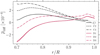Fig. 1. Density difference between regions at 60° above the equator and the equator.

Snapshots of the final state of the radial (convective) velocity near the surface of the star are given in Fig. 2 for simulations D1 and D3, which are also representative of the other runs within our set of simulations. The series of runs C and D correspond to fast rotators, and the convective cells are therefore very small toward medium to high latitudes, whereas they become elongated near the equator. This is a common phenomenon obtained in simulations of stellar convection (see, e.g., Viviani et al. 2018) and is consistent with the Taylor-Proudman balance. The result for D3 is very similar as for D1, but it is not identical. While both runs were evolved until the same time, an identical result is not expected because the dynamics are nonlinear and because the centrifugal force causes perturbations within the star. On the other hand, and even though in principle the strength of the centrifugal force is quite significant in run D3, the impact on the flow pattern appears to be relatively minor.

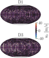Fig. 2. Mollweide projections of radial velocity near the surface for runs D1 and D3.

Similar projections, now for the radial component of the magnetic field, are presented in Fig. 3. In run D1, clear nonaxisymmetric structures are present that extend throughout each hemisphere. Nonaxisymmetric structures seem to be somewhat smaller in run D3, that is, an m = 2 mode is also present. The amplitude of B_r remains very similar.

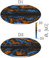Fig. 3. Mollweide projections of radial magnetic field near the surface for runs D1 and D3.

We decomposed the radial velocity field at the surface of selected runs into spherical harmonics and calculated the normalized convective power spectra as

$$\begin{array}{c}\hfill P_{\mathrm{kin}}=\frac{E_{\mathrm{kin},l}}{{\sum }_l{E}_{\mathrm{kin},l}},\end{array}$$(20)

where E_kin,  l is the kinetic energy of the lth degree. This is shown in Fig. 4, where we plot P as a function of l up to l_max = 288. This is the maximum resolution we can achieve because we used 576 grid points along the ϕ direction. The convective power peak is shifted toward higher l for higher rotation rates, but the centrifugal force has no significant influence on it, even in the extreme case of run D3. We note that the contribution of the polar caps, which are not part of the computational domain, are not included in the spherical harmonic decomposition or in the power spectra.

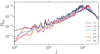Fig. 4. Normalized convective power spectra for runs C1, C2, C3, D1, D2, and D3.

In Fig. 5 we show the time-averaged and azimuthally averaged angular velocity normalized with the angular velocity of the rotating frame for simulations with different rotation rates and with and without the centrifugal force. In set D, where the angular velocity is higher in general, we find that stellar differential rotation is reduced compared with set C, which is expected for more rapidly rotating runs (e.g., Kitchatinov & Rüdiger 1995; Viviani et al. 2018). Measures of the radial and latitudinal differential rotation are shown in Table 1. They are defined as

$$\begin{array}{cc}\hfill {\mathrm{\Delta }}_{\mathrm{\Omega }}^{(r)}& =\frac{{\mathrm{\Omega }}_{\mathrm{eq}}-{\mathrm{\Omega }}_{\mathrm{bot}}}{{\mathrm{\Omega }}_{\mathrm{eq}}},\hfill \end{array}$$(21)

$$\begin{array}{cc}\hfill {\mathrm{\Delta }}_{\mathrm{\Omega }}^{({60}^{°})}& =\frac{{\mathrm{\Omega }}_{\mathrm{eq}}-{\mathrm{\Omega }}_{{60}^{°}}}{{\mathrm{\Omega }}_{\mathrm{eq}}},\hfill \end{array}$$(22)

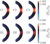Fig. 5. Mean rotation rate averaged over the last 80 yr of the simulation and normalized to the rotation rate of the star. ⟨...⟩t denotes the average over time.

respectively. Here, Ω_eq, Ω_bot, and Ω_60° are the angular velocities at the equator near the surface, at the equator near the bottom of the convective zone, and near the surface at a latitude of 60°, respectively. The time-averaged radial differential rotation remains practically the same within each set. The time-averaged radial and latitudinal differential rotation only changes appreciably in run D3 by a factor of four and two, respectively, where we enhanced the centrifugal force. We fail to find strong evidence for a direct effect of the centrifugal force from the time averages, however. We also show the rms values of the fluctuations (instantaneous minus average) of ${\mathrm{\Delta }}_{\mathrm{\Omega }}^{(r)}$ and ${\mathrm{\Delta }}_{\mathrm{\Omega }}^{({60}^{°})}$ in the last two columns of Table 1. In general, there is a tendency of increased fluctuations when the centrifugal force is included and when its amplitude is larger.

Observations of the rapidly rotating K2 dwarf V471 Tau, which is a PCEB rotating at about 50 times faster than the Sun, show that it has a solar-like differential rotation (Zaire et al. 2022). The surface differential rotation is about ${\mathrm{\Delta }}_{\mathrm{\Omega }}^{({60}^{°})}$ = 3.7 × 10⁻³, as measured from the shearing of brightness inhomogeneities (Stokes I), and ${\mathrm{\Delta }}_{\mathrm{\Omega }}^{({60}^{°})}$ = 2.6 × 10⁻³ from magnetic structures (Stokes V). The sign of the differential rotation agrees with our simulations, and the amplitude here is about ten times smaller. We note, however, that in some cases, the instantaneous value of ${\mathrm{\Delta }}_{\mathrm{\Omega }}^{({60}^{°})}$ can be as high as 10⁻³.

3.2. Gravitational quadrupole moment

We analyzed the xx-component of the gravitational quadrupole moment for runs C1, C2, and C3 and for runs D1, D2, and D3. It is defined as

$$\begin{array}{c}\hfill Q_{\mathit{ij}}=I_{\mathit{ij}}-\frac{1}{3}{\delta }_{\mathit{ij}}\mathrm{Tr}I,\end{array}$$(23)

where

$$\begin{array}{c}\hfill I_{\mathit{ij}}={\displaystyle \int }\rho (\mathit{x})x_i{x}_j\mathrm{d}V\end{array}$$(24)

is the inertia tensor, with ρ being the density, and x_i, x_j are Cartesian coordinates. The time evolution of Q_xx for all runs is shown in Fig. 6. Their yy- and zz-components evolve very similarly, as demonstrated in Navarrete et al. (2020). The average quadrupole moment and its standard deviation are summarized in Table 2 for each simulation.

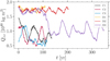Fig. 6. Qxx component of the gravitational quadrupole moment as a function of time for all runs.

For series C with the somewhat lower rotation rate, the average value of the quadrupole moment appears to be slightly lower (∼7 − 9 × 10³⁹ kg m²) than in series D (∼1 − 2 × 10⁴⁰ kg m²), while the standard deviation appears to be larger for series C (∼2 × 10³⁹ kg m²) than for series D (∼6 − 10 × 10³⁸ kg m²). Within the range of uncertainty, the mean value and the variation appear to be similar within the set of simulations C1, C2, and C3, as well as within the set of simulations D1, D2, and D3. This is to say that the centrifugal force does not appear to affect the mean value of the quadrupole moment very strongly. The standard deviation appears to be almost unaffected by the centrifugal force within set C. Some more coherent variations are visible in run D2 and particularly in run D3, where the centrifugal force is the strongest of all runs. We note further that the drop of the mean quadrupole moment value in run D3 around t = 100 yr coincides with a decrease in the mean radial magnetic field around the same time, which is shown in Fig. 7. The magnetic field structure and its time evolution is clearly different in all simulations, and we also find differences in simulations with and without the centrifugal force. It is difficult to assess, however, whether the origin of this difference is essentially related to a possible bimodality of the solutions or if the centrifugal force specifically introduces a different type of behavior. Overall, the results thus indicate that the stellar quadrupole moment is not very sensitive to the centrifugal force.

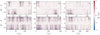Fig. 7. Mean (azimuthally averaged) radial magnetic field near the surface for all runs.

4. Discussion and conclusions

We presented a series of numerical simulations with which we investigated stellar dynamos of solar-mass stars with angular velocities of 20 and 30 times the solar rotation. The simulations were performed using the enhanced luminosity method (Brandenburg et al. 2005; Käpylä et al. 2013; Navarrete et al. 2020) to avoid prohibitively large gaps in the relevant timescales. This entails the use of correspondingly enhanced rotation rates to ensure a realistic Coriolis number in the simulations, which is required to reach realistic magnitudes of the drivers of dynamo action, such as the α and Ω effects. We included and varied the strength of the centrifugal force in these simulations, including cases without the centrifugal force or where the strength of the centrifugal force was enhanced by an order of magnitude.

The centrifugal force in general causes perturbations during the nonlinear evolution, so that the models evolve differently in the details, although it is hard to identify clear systematic effects. We note in particular that the averaged radial density profile of the stars remains almost unchanged, while the density difference between the equator and high latitudes (60°) changes by a relative amount of 10⁻⁴. We see some difference between the distribution of axisymmetric and nonaxisymmetric modes of the dynamo, and the convective power spectra are affected by the strength of the angular velocity, but not so much by the centrifugal force. Except for the behavior of the density difference (Fig. 1), we found no clear systematic effects that were due to the centrifugal force.

We similarly find that the mean and standard deviation of the quadrupole moment depend more strongly on the angular velocity, while the influence of the centrifugal force is weak or almost nonexistent, even in the simulation in which the centrifugal force term is enhanced by an order of magnitude. This is highly relevant because in the original models proposed by Applegate (1992), the centrifugal force term was supposed to give rise to the variation in stellar quadrupole moment, while here we find similar variations regardless of the presence of the centrifugal force. This suggests that the centrifugal force plays only a minor role in causing this variation, as the overall flow patterns within the star are driven by more complex dynamics resulting from the nonlinear evolution of the system. Adopting the parameters of V471 Tau (Völschow et al. 2016) and inserting the quadrupole variations that we find here into the framework of Applegate (1992; see Navarrete et al. 2022), that is,

$$\begin{array}{c}\hfill \frac{\mathrm{\Delta }P}{P}=-9\frac{\mathrm{\Delta }{Q}_{\mathit{xx}}}{M{a}^2},\end{array}$$(25)

where ΔP/P is the variation of the period of the binary, ΔQ_xx is the variation of the quadrupole moment, M is the stellar mass, and a is the binary separation, we obtain period variations of the order of 10⁻⁸...10⁻⁹, whereas the amplitude of the period variation of close binaries is around 10⁻⁶...10⁻⁷ (see, e.g., Völschow et al. 2018), and about 8.5 × 10⁻⁷ for V471 Tau (Zaire et al. 2022). While the original model was useful to motivate the possible origin of the fluctuations via magnetic activity, it appears to have difficulties overall in explaining the observed magnitude of the variations, and the centrifugal force is unlikely to be the main driver of the variations.

As in our previous studies, we chose to apply our results to V471 Tau alone because of the similarities between the extension of the convective zones of our model and the real K2 dwarf. We can roughly rescale the gravitational quadrupole moment variations obtained here to a target star of mass $\stackrel{\sim }{M}$ and radius $\stackrel{\sim }{R}$ by assuming that the quadrupole moment scales with the stellar inertial moment, that is,

$$\begin{array}{c}\hfill \mathrm{\Delta }{\stackrel{\sim }{Q}}_{\mathit{xx}}=\frac{\stackrel{\sim }{M}{\stackrel{\sim }{R}}^2}{M{R}^2}\mathrm{\Delta }{Q}_{\mathit{xx}},\end{array}$$(26)

where M and R are the mass and radius of our simulated star. Choosing the parameters of NN Ser of $\stackrel{\sim }{M}=0.111M_{\odot }$, $\stackrel{\sim }{R}=0.149R_{\odot }$, and a = 0.934R_⊙ (Völschow et al. 2016) yields

$$\begin{array}{c}\hfill \frac{\mathrm{\Delta }P}{P}=2.34\times {10}^{-9},\end{array}$$(27)

which is a few hundred times lower than the value estimated from observations (Völschow et al. 2016). This number should be taken with extreme caution, however. A potential error source is the missing effect of rotation in Eq. (26). The value of $\mathrm{\Delta }{\stackrel{\sim }{Q}}_{\mathit{xx}}$ is a rather crude estimate and results from self-consistent simulations that will be presented elsewhere.

As in previous work (e.g., Navarrete et al. 2020, 2022), our simulations confirm that MHD simulations of stellar dynamos naturally produce an evolution of the stellar quadrupole moment, including one varying and one approximately constant component. The time-varying component may be somewhat too small to explain the observed ETVs. As suggested in models by Applegate (1989) and Lanza (2020), a roughly constant component might produce the variations caused by spin-orbit coupling via libration or circulation (see also the discussion in Navarrete et al. 2022). As our simulations indeed show a mean and a fluctuating part of the quadrupole moment, the observed real variation may well consist of a superposition of the two components, where the relative strength may depend on the specific system and its parameters. As has been demonstrated by Navarrete et al. (2020), the presence of magnetic fields is crucial because purely hydrodynamic simulations only produce short-term variations on the sound-crossing timescale of the star, but no longer-term variations on timescales of years or decades.

From the results obtained here, we thus conclude that neither the thin-shell model by Applegate (1992) nor the finite-shell model by Brinkworth et al. (2006) correctly describes the origin of the quadrupole moment variation because they both assume it to originate in the centrifugal force and in an internal redistribution of the angular velocity, while in our simulations, a change in centrifugal force term does not lead to any appreciable change in the mean or fluctuating component of the quadrupole. The physics causing these variations thus requires modeling the stellar dynamo with compressible MHD in three dimensions.

Another possibility is given by hybrid solutions in which ETVs receive contributions of magnetic origin and from planets. Mai & Mutel (2022) considered such a scenario for three PCEBs as neither planets nor the Applegate mechanism can fully account for ETVs. We conclude by encouraging studies of the detection of circumbinary planets around PCEBs as well as Zeeman-Doppler imaging of their main-sequence components. The combination of these subjects will help us constrain the planetary orbits and masses, and to understand to which extent we can use ETVs to study stellar magnetic fields.

Acknowledgments

We thank the referee for a detailed review and helpful comments that improved the manuscript. F.H.N. acknowledges financial support from the DAAD (Deutscher Akademischer Austauschdienst; code 91723643) for his doctoral studies. D.R.G.S. gratefully acknowledges support by the ANID BASAL projects ACE210002 and FB210003, as well as via the Millenium Nucleus NCN19-058 (TITANs). D.R.G.S. and C.A.O.R. thank for funding via Fondecyt Regular (project code 1201280). P.J.K. acknowledges financial support by the Deutsche Forschungsgemeinschaft Heisenberg programme (grant No. KA 4825/4-1).

References

All Tables

All Figures

	Fig. 1. Density difference between regions at 60° above the equator and the equator.
In the text

	Fig. 2. Mollweide projections of radial velocity near the surface for runs D1 and D3.
In the text

	Fig. 3. Mollweide projections of radial magnetic field near the surface for runs D1 and D3.
In the text

	Fig. 4. Normalized convective power spectra for runs C1, C2, C3, D1, D2, and D3.
In the text

	Fig. 5. Mean rotation rate averaged over the last 80 yr of the simulation and normalized to the rotation rate of the star. ⟨...⟩t denotes the average over time.
In the text

	Fig. 6. Qxx component of the gravitational quadrupole moment as a function of time for all runs.
In the text

	Fig. 7. Mean (azimuthally averaged) radial magnetic field near the surface for all runs.
In the text

References

- Applegate, J. H. 1989, ApJ, 337, 865 [NASA ADS] [CrossRef] [Google Scholar]
- Applegate, J. H. 1992, ApJ, 385, 621 [Google Scholar]
- Applegate, J. H., & Patterson, J. 1987, ApJ, 322, L99 [NASA ADS] [CrossRef] [Google Scholar]
- Beuermann, K., Hessman, F. V., Dreizler, S., et al. 2010, A&A, 521, L60 [NASA ADS] [CrossRef] [EDP Sciences] [Google Scholar]
- Beuermann, K., Breitenstein, P., Debski, B., et al. 2012, A&A, 540, A8 [NASA ADS] [CrossRef] [EDP Sciences] [Google Scholar]
- Beuermann, K., Dreizler, S., & Hessman, F. V. 2013, A&A, 555, A133 [NASA ADS] [CrossRef] [EDP Sciences] [Google Scholar]
- Bours, M. C. P., Marsh, T. R., Parsons, S. G., et al. 2016, MNRAS, 460, 3873 [Google Scholar]
- Brandenburg, A., Chan, K. L., Nordlund, Å., & Stein, R. F. 2005, Astron. Nachr., 326, 681 [NASA ADS] [CrossRef] [Google Scholar]
- Brinkworth, C. S., Marsh, T. R., Dhillon, V. S., & Knigge, C. 2006, MNRAS, 365, 287 [Google Scholar]
- Decampli, W. M., & Baliunas, S. L. 1979, ApJ, 230, 815 [NASA ADS] [CrossRef] [Google Scholar]
- Hardy, A., Schreiber, M. R., Parsons, S. G., et al. 2015, ApJ, 800, L24 [NASA ADS] [CrossRef] [Google Scholar]
- Käpylä, P. J., Mantere, M. J., Cole, E., Warnecke, J., & Brandenburg, A. 2013, ApJ, 778, 41 [CrossRef] [Google Scholar]
- Käpylä, P. J., Gent, F. A., Olspert, N., Käpylä, M. J., & Brandenburg, A. 2020, Geophys. Astrophys. Fluid Dyn., 114, 8 [CrossRef] [Google Scholar]
- Kitchatinov, L. L., & Rüdiger, G. 1995, A&A, 299, 446 [NASA ADS] [Google Scholar]
- Lanza, A. F. 2006, MNRAS, 369, 1773 [NASA ADS] [CrossRef] [Google Scholar]
- Lanza, A. F. 2020, MNRAS, 491, 1820 [NASA ADS] [Google Scholar]
- Mai, X., & Mutel, R. L. 2022, MNRAS, 513, 2478 [NASA ADS] [CrossRef] [Google Scholar]
- Marsh, T. R., & Pringle, J. E. 1990, ApJ, 365, 677 [NASA ADS] [CrossRef] [Google Scholar]
- Matese, J. J., & Whitmire, D. P. 1983, A&A, 117, L7 [NASA ADS] [Google Scholar]
- Mustill, A. J., Marshall, J. P., Villaver, E., et al. 2013, MNRAS, 436, 2515 [NASA ADS] [CrossRef] [Google Scholar]
- Navarrete, F. H., Schleicher, D. R. G., Zamponi Fuentealba, J., & Völschow, M. 2018, A&A, 615, A81 [NASA ADS] [CrossRef] [EDP Sciences] [Google Scholar]
- Navarrete, F. H., Schleicher, D. R. G., Käpylä, P. J., et al. 2020, MNRAS, 491, 1043 [Google Scholar]
- Navarrete, F. H., Käpylä, P. J., Schleicher, D. R. G., Ortiz, C. A., & Banerjee, R. 2022, A&A, 663, A90 [NASA ADS] [CrossRef] [EDP Sciences] [Google Scholar]
- Ogilvie, G. I., & Lin, D. N. C. 2007, ApJ, 661, 1180 [Google Scholar]
- Pencil Code Collaboration (Brandenburg, A., et al.) 2021, J. Open Source Software, 6, 2807 [CrossRef] [Google Scholar]
- Schleicher, D. R. G., & Dreizler, S. 2014, A&A, 563, A61 [NASA ADS] [CrossRef] [EDP Sciences] [Google Scholar]
- Vaccaro, T. R., Wilson, R. E., Van Hamme, W., & Terrell, D. 2015, ApJ, 810, 157 [NASA ADS] [CrossRef] [Google Scholar]
- Viviani, M., Warnecke, J., Käpylä, M. J., et al. 2018, A&A, 616, A160 [NASA ADS] [CrossRef] [EDP Sciences] [Google Scholar]
- Völschow, M., Banerjee, R., & Hessman, F. V. 2014, A&A, 562, A19 [NASA ADS] [CrossRef] [EDP Sciences] [Google Scholar]
- Völschow, M., Schleicher, D. R. G., Perdelwitz, V., & Banerjee, R. 2016, A&A, 587, A34 [NASA ADS] [CrossRef] [EDP Sciences] [Google Scholar]
- Völschow, M., Schleicher, D. R. G., Banerjee, R., & Schmitt, J. H. M. M. 2018, A&A, 620, A42 [NASA ADS] [CrossRef] [EDP Sciences] [Google Scholar]
- Zahn, J. P., & Bouchet, L. 1989, A&A, 223, 112 [NASA ADS] [Google Scholar]
- Zaire, B., Donati, J. F., & Klein, B. 2022, MNRAS, 513, 2893 [NASA ADS] [CrossRef] [Google Scholar]
- Zorotovic, M., & Schreiber, M. R. 2013, A&A, 549, A95 [NASA ADS] [CrossRef] [EDP Sciences] [Google Scholar]
All Tables
Summary of the rms value and standard deviation of the quadrupole moment obtained in the simulations.