| Issue |
A&A
Volume 678, October 2023
|
|
|---|---|---|
| Article Number | A82 | |
| Number of page(s) | 11 | |
| Section | Stellar structure and evolution | |
| DOI | https://doi.org/10.1051/0004-6361/202244666 | |
| Published online | 10 October 2023 | |
Simulations of dynamo action in slowly rotating M dwarfs: Dependence on dimensionless parameters
1
Departamento de Astronomía, Facultad de Ciencias Físicas y Matemáticas, Universidad de Concepción, Av. Esteban Iturra s/n Barrio Universitario, Casilla 160-C, Chile
e-mail: This email address is being protected from spambots. You need JavaScript enabled to view it.
2
Leibniz-Institut für Sonnenphysik (KIS), Schöneckstr. 6, 79104 Freiburg, Germany
3
Institut für Astrophysik und Geophysik, Georg-August-Universität Göttingen, Friedrich-Hund-Platz 1, 37077 Göttingen, Germany
4
Nordita, KTH Royal Institute of Technology and Stockholm University, 10691 Stockholm, Sweden
5
Hamburger Sternwarte, Universität Hamburg, Gojenbergsweg 112, 21029 Hamburg, Germany
Received:
2
August
2022
Accepted:
2
August
2023
Abstract
Aims. The aim of this study is to explore the magnetic and flow properties of fully convective M dwarfs as a function of rotation period Prot and magnetic Reynolds ReM and Prandlt numbers PrM.
Methods. We performed three-dimensional simulations of fully convective stars using a star-in-a-box set-up. This set-up allows global dynamo simulations in a sphere embedded in a Cartesian cube. The equations of non-ideal magnetohydrodynamics were solved with the PENCIL CODE. We used the stellar parameters of an M5 dwarf with 0.21 M⊙ at three rotation rates corresponding to rotation periods (Prot) of 43, 61, and 90 days, and varied the magnetic Prandtl number in the range from 0.1 to 10.
Results. We found systematic differences in the behaviour of the large-scale magnetic field as functions of rotation and PrM. For the simulations with Prot = 43 days and PrM ≤ 2, we found cyclic large-scale magnetic fields. For PrM > 2, the cycles vanish and the field shows irregular reversals. In the simulations with Prot = 61 days for PrM ≤ 2, the cycles are less clear and the reversal are less periodic. In the higher PrM cases, the axisymmetric mean field shows irregular variations. For the slowest rotation case with Prot = 90 days, the field has an important dipolar component for PrM ≤ 5. For the highest PrM the large-scale magnetic field is predominantly irregular at mid-latitudes, with quasi-stationary fields near the poles. For the simulations with cycles, the cycle period length slightly increases with increasing ReM.
Key words: convection / dynamo / stars: magnetic field / stars: low-mass / magnetohydrodynamics (MHD)
© The Authors 2023
 Open Access article, published by EDP Sciences, under the terms of the Creative Commons Attribution License (https://creativecommons.org/licenses/by/4.0), which permits unrestricted use, distribution, and reproduction in any medium, provided the original work is properly cited.
This article is published in open access under the Subscribe to Open model. This email address is being protected from spambots. You need JavaScript enabled to view it. to support open access publication.
1. Introduction
Magnetic fields in stars have been studied both theoretically and through observations, particularly magnetic fields of solar-type main-sequence stars (e.g., Brun & Browning 2017, and references therein). M dwarfs are low-mass main-sequence stars whose structure undergoes a transition from fully convective for masses up to 0.35 M⊙ to solar-like (radiative core and convective envelope) for higher masses (Chabrier & Baraffe 1997). These stars are found to be magnetically active, as shown by Saar & Linsky (1985), who confirmed surface magnetic activity for M dwarfs with infrared measurements. Today there is considerable observational evidence of magnetic activity in M dwarfs that shows magnetic field strengths reaching up to a few kG (see Kochukhov 2021, and references therein). Because of the lack of a tachocline, the shear layer between the radiative and convective zones, fully convective M dwarfs are quite interesting from the point of view of dynamo theory and can help us to understand whether a tachocline has a strong impact on the dynamo itself. In this context, Wright & Drake (2016) report that the X-ray emission of fully and partially convective stars follows a similar trend to the Rossby number Ro = Prot/τ, which is the ratio of the rotation period to convective turnover time, and which measures the rotational influence on convective flows. It was found that the X-ray emission increases with decreasing Ro until Ro ≈ 0.1, and for smaller Ro the X-ray luminosity saturates. Newton et al. (2017) find a similar trend, a saturated relation between the chromospheric Hα emission and Ro for rapidly rotating M dwarfs and a power-law decay of the Hα emission with increasing Ro for slowly rotating stars. The transition occurs near Ro = 0.2. In addition, Doppler and Zeeman-Doppler inversions have revealed that fully convective M dwarfs often show large-scale magnetic fields, and that for rapid enough rotation both dipolar and multipolar fields are possible (e.g., Morin et al. 2010; Kochukhov 2021). Furthermore, Klein et al. (2021) found that the fully convective star Proxima Centauri has a seven-year activity cycle.
Numerical simulations of stars are performed to achieve a better understanding of their magnetic fields, dynamos, and convection as functions of stellar parameters and dimensionless quantities, such as the magnetic Prandtl number, which is an intrinsic property of the fluid defined by the ratio of kinematic viscosity ν to resistivity η of the plasma. Some authors have performed magnetohydrodynamic (MHD) simulations of fully convective M dwarfs, which are particularly interesting for comparison with solar dynamo models due to the lack of a tachocline. The first simulations of fully convective M dwarfs were presented by Dobler et al. (2006), who used a star-in-a-box model to study dynamos as a function of rotation. They found predominantly quasi-static large-scale magnetic fields and typically weak or anti-solar differential rotation with faster poles and a slower equator. These simulations had relatively modest fluid and magnetic Reynolds numbers as well as low density-stratification. Browning (2008) presented simulations of fully convective M dwarfs using the anelastic magnetohydrodynamic equations, considering a spherical domain extending from 0.08 to 0.96 stellar radius, finding magnetic fields with significant axisymmetric components. In simulations without magnetic fields, the differential rotation is strong and solar-like with a fast equator and slow poles; instead, in magnetic simulations it is reduced, and tends to a solid-body rotation in the most turbulent magnetohydrodynamical simulations. A similar numerical approach was taken in the studies of Yadav et al. (2015, 2016) who used strongly stratified anelastic simulations to study the coexistence of dipolar and multipolar dynamos and cyclic solutions at relatively slow rotation corresponding to a parameter regime similar to that of Proxima Centauri. More recently, Brown et al. (2020) performed simulations of fully convective M dwarfs in spherical coordinates, finding cyclic hemispheric dynamos in their models.
The rotation period of the star Prot is a key factor that determines the nature of the dynamo. This is evidenced by observational studies of M dwarfs, which demonstrate that with decreasing Prot the magnetic field strength increases (e.g., Wright et al. 2018; Reiners et al. 2022). This has also been shown numerically by Käpylä (2021), among others, who used a star-in-a-box model for fully convective stars and found increasing magnetic field strength with decreasing rotation period. Furthermore, different dynamo modes were found as a function of rotation in that work. Slowly rotating stars have mostly axisymmetric and quasi-steady large-scale magnetic fields; for intermediate rotation the large-scale field is mostly axisymmetric and cyclic, and for rapid rotation the large-scale magnetic fields are predominantly non-axisymmetric with a dominant m = 1 mode. As demonstrated by Käpylä (2021), the large-scale dynamo is sustained even in the absence of a tachocline. In this sense, the work by Bice & Toomre (2020) using simulations of early M dwarfs supports the hypothesis that the tachocline is not necessary for producing strong toroidal magnetic fields, although it may generate stronger fields in faster rotators.
In this paper we present three-dimensional MHD simulations of fully convective M dwarfs with the star-in-a-box set-up described in Käpylä (2021; see also Dobler et al. 2006). Our main goal is to explore the dependence on dimensionless parameters, in particular the magnetic Prandtl and Reynolds numbers PrM and ReM, which are crucial ingredients for dynamos and plasmas in general. High and low values of PrM and ReM lead to very different dynamo scenarios; at low PrM the magnetic energy is dissipated in the inertial range of the flow and small-scale dynamo action requires a much higher ReM to be excited (e.g., Schekochihin et al. 2007; Käpylä et al. 2018). On the other hand, stars typically have PrM ≪ 1 and ReM ≫ 1 (e.g., Augustson et al. 2019; Jermyn et al. 2022). Our simulations were performed for a set of rotation periods Prot ranging from 43 to 90 days, the latter being the rotation period of Proxima Centauri, and for values of PrM and ReM ranging from 0.1 to 10 and 21 to over 1400, respectively, which is the numerically feasible range for this type of simulation. The methods and model are described in Sect. 2, while the description and analysis of the results is provided in Sect. 3. We discuss the conclusions in Sect. 4.
2. Methods
We used the star-in-a-box model described in Käpylä (2021), which is based on the set-up of Dobler et al. (2006). The model allows dynamo simulations of entire stars. In the present scenario we used a sphere of radius R that is enclosed in a cube with side 2.2 R. We solved the induction, continuity, momentum, and energy conservation equations:
 (1)
(1)
 (2)
(2)
 (3)
(3)
![Mathematical equation: $$ \begin{aligned} T \frac{\mathrm{D} s}{\mathrm{D} t}&=\frac{1}{\rho }\left[\mathcal{H} - \mathcal{C} - \boldsymbol{\nabla } \cdot \left(\boldsymbol{F}_{\rm rad} + \boldsymbol{F}_{\rm SGS} \right) \right] + 2\nu \boldsymbol{\mathsf{S}}^2 + \frac{\mu _0 \eta \boldsymbol{J}^2}{\rho }.\end{aligned} $$](/articles/aa/full_html/2023/10/aa44666-22/aa44666-22-eq4.gif) (4)
(4)
Here A is the magnetic vector potential; u is the velocity field; B = ∇ × A is the magnetic field; μ0 is the magnetic permeability of vacuum; η is the magnetic diffusivity; ρ is the density of the fluid; D/Dt = ∂/∂t + u·∇ is the advective derivative; T is the temperature; Φ is the gravitational potential; p is the pressure; ν is the kinematic viscosity; s is the specific entropy; J = ∇ × B/μ0 is the current density;  is the rotation vector (with Ω0 being the mean angular velocity of the star and
  the unit vector along the rotation axis); 𝖲 is the traceless rate-of-strain tensor
 (5)
(5)
where the commas denote differentiation; ℋ and 𝒞 describe heating and cooling; and fd describes the damping of flows outside the star (see Käpylä 2021, for more details). The radiative flux is given by
 (6)
(6)
where K corresponds to the Kramers opacity law, where its power law exponents are the same as in Käpylä (2021). The subgrid-scale (SGS) entropy flux FSGS damps fluctuations near the grid scale, but contributes only negligibly to the net energy transport. It is given by
 (7)
(7)
where χSGS is the SGS diffusion coefficient,  is the entropy fluctuation, and
  is a running temporal mean of the entropy. We note that the SGS flux used here does not include the temperature T. This form of the SGS flux is appropriate if the entropy equation has been solved, whereas the T factor appears in the SGS term if the corresponding energy equation has been solved (Rogachevskii & Kleeorin 2015).
The simulations were run with the PENCIL CODE1 (Brandenburg 2021), which is a high-order finite-difference code for solving partial differential equations with primary applications in compressible astrophysical magnetohydrodynamics.
2.1. Dimensionless parameters
Each simulation is characterised by various dimensionless numbers. These parameters are usually order of magnitude ratios of various terms in the MHD equations or of the corresponding timescales.
The effect of rotation relative to viscosity is measured by the Taylor number, given by
 (8)
(8)
The Coriolis number is a measure of the influence of rotation on the flow
 (9)
(9)
where urms is the volume-averaged root mean square velocity and kR = 2π/R is the scale of the largest convective eddies. Another definition of the Coriolis number used in other studies (e.g., Brown et al. 2020; Käpylä 2021) is based on the vorticity and considers the local length scale. This is defined by
 (10)
(10)
where ωrms is the volume averaged rms vorticity, with ω = ∇ × u. The fluid and magnetic Reynolds numbers, SGS and magnetic Prandtl numbers, and SGS Péclet numbers are defined as
 (11)
(11)
 (12)
(12)
2.2. Physical units and non-dimensional quantities
We modelled a main-sequence dwarf star (M5) with the same stellar parameters as in Dobler et al. (2006) and Käpylä (2021). The mass, radius, and luminosity of the star are M⋆ = 0.21 M⊙, R⋆ = 0.27 R⊙, and L⋆ = 0.008 L⊙, respectively. We used an enhanced luminosity approach (Käpylä et al. 2020) to reduce the gap between the thermal and dynamical timescales, such that fully compressible simulations are feasible. This implies that the results need to be scaled suitably for comparison with real stars. The conversion factor between the rotation rate, length, time, velocity, and magnetic fields in the simulation and in physical units are the same as those used by Käpylä (2021; see their Appendix A). Non-dimensional quantities were obtained by using the stellar radius as the unit of length [x]=R. Time is given in terms of the free-fall time  , the unit of velocity is [U]=R/τff, and magnetic fields are given in terms of the equipartition field strength
  , where ⟨.⟩ stands for time and volume averaging.
3. Results
We present a set of 3D MHD simulations in the slow to intermediate rotation regime with global Coriolis number Co ranging between 3.1 and 12.9 (see Table 1). The rotation rates are  , 0.7, and 0.5 (which correspond to Prot = 43, 61, and 90 days) in sets A, B, and C, respectively. The magnetic Prandtl number PrM varies between 0.1 and 10 in set A and between 0.5 and 10 in sets B and C.
Simulation parameters.
3.1. Flow properties
3.1.1. Differential rotation and meridional circulation
The averaged rotation rate in cylindrical coordinates is given by
 (13)
(13)
where ϖ = r sin θ is the cylindrical radius and where the overbar denotes azimuthal averaging. The averaged meridional flow is given by
 (14)
(14)
The angular velocity varies with depth and also with latitude. A way to quantify this is by measuring the amplitude of the radial and latitudinal differential rotation with
 (15)
(15)
 (16)
(16)
where the subscripts top, bot, eq, and  respectively correspond to R = 0.9R, r = 0.1R, θ = 0°, and an average of
  for latitudes +θ and −θ in spherical coordinates.
The values of  and
and  are listed in Table 2. Positive values of
  indicate solar-like differential rotation. We find that
  has a tendency to decrease with increasing ReM, which is equivalent to an increasing PrM (second column of Table 2). Figure 1 shows
  as a function of ReM for sets A (circles), B (squares), and C (triangles) confirming the decreasing trend as a function of ReM. The red circles show simulations without dynamos (A8 and A12) and low magnetic Reynolds numbers, where
  is higher. This reduction or quenching of the differential rotation by magnetic fields especially at high ReM has been shown by various simulations, for example in Brun et al. (2004), Schrinner et al. (2012), and Käpylä et al. (2017). The differential rotation profiles for three representative simulations A1, A16, and A8 are shown in Fig. 2. The rotation profile in run A1 is solar-like; the profile is similar in the rest of the simulations with PrM ≤ 2. In run A16 with PrM = 10 the amplitude of the latitudinal differential rotation is positive, whereas the amplitude of the radial differential rotation is negative since the angular velocity does not change considerably with depth at the equator. The middle panel of Fig. 2 shows that the rotation rate at the equator is in fact higher than average almost everywhere and the negative value of
  is due to the slower-than-average rotation only very near the surface. Therefore, the differential rotation is solar-like. Another method for classifying the rotation profile (solar-like or anti-solar) is to use the mean rotation profile at the equator, which, as indicated in Käpylä (2023), can help prevent erroneous conclusions. Furthermore, the profiles in Fig. 2 are symmetric with respect to the equator, as in the other simulations performed in this work.
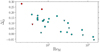 |
Fig. 1. Amplitude of radial differential rotation as a function of magnetic Reynolds number for simulations of sets A (circles), B (squares), and C (triangles). Cyan and red is for simulations with dynamo and without dynamo, respectively. |
Amplitudes of the temporally and azimuthally averaged angular velocity  .
.
The global Coriolis number (see Eq. (9)) in the current simulations ranges from 3.1 to 13. All of our runs show solar-like differential rotation, which is consistent with Käpylä (2021), where the shift from anti-solar to solar-like differential rotation occurs for Coriolis number between 0.7 and 2. This is also consistent with the simulations of spherical shell convection by Viviani et al. (2018), which show that the transition occurs at around Co = 3 (see Table 5 in their work). More recently, Käpylä (2023) found that the transition from anti-solar to solar-like differential rotation depends on the subgrid-scale Prandtl number (PrSGS), such that solar-like differential rotation is more difficult to obtain at high PrSGS than at PrSGS ≤ 1. In this work all the simulations have PrSGS ≤ 1.
Simulations A8, A12, and C2 do not have dynamos, and they are considered to be kinematic cases. The right panel of Fig. 2 displays the rotation profile for simulation A8. It demonstrates that a faster-than-average angular velocity spans a broader latitudinal range and a narrower radial range when compared to dynamo simulations. This depicts the influence of a magnetic field on differential rotation. In the regime PrM < 2 of our simulations, the meridional flow is composed of multiple small cells, while in the regime PrM ≥ 2 the pattern is composed of two to three large cells which are symmetric with respect to the equator. The maximum values of the normalised meridional flow amplitude,  , in the cases shown in Fig. 2 correspond to
  , 0.005, and 0.023 for simulations A1, A16, and A8, respectively. The rms value of the meridional velocity is given in the fifth column of Table 2. In the simulations with no dynamo, A8, A12, and C2 (A8 in right panel in Fig. 2), the meridional circulation also exhibits similar multiple patterns, which are also symmetric with respect to the equator.
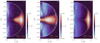 |
Fig. 2. Normalised time-averaged mean angular velocity |


3.1.2. Power spectra and kinetic helicity
To characterise the convective flows we calculated the normalised kinetic energy power spectra (e.g., Viviani et al. 2018; Navarrete et al. 2022) from
 (17)
(17)
where Ekin, ℓ is the kinetic energy of the spherical harmonic degree ℓ, which is calculated from the decomposition of the radial velocity field at the surface into spherical harmonics. Figure 3 shows Pkin as a function of ℓ for selected simulations. For the simulations with lower rotation rates and large-scale dynamos, the convective power is slightly shifted towards lower ℓ, with peaks between 16 and 20 for set A, 12 and 15 for set B, and 7 and 15 for set C. In simulations with no dynamo, the peak is at considerably larger scales at ℓ = 4. This demonstrates the suppression of large-scale convective flows by magnetic fields. This is similar to results from recent solar-like simulations that suggest that suppression of large-scale convection may be important to maintain a solar-like rotation profile in the Sun (e.g., Hotta et al. 2022; Käpylä 2023). Furthermore, the large-scale convective amplitudes are in general higher in cases with slower rotation, in agreement with linear theory (Chandrasekhar 1961) and various earlier simulations (Featherstone & Hindman 2016; Viviani et al. 2018; Navarrete et al. 2022).
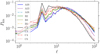 |
Fig. 3. Normalised convective power as a function of ℓ for simulations A10, A13, A16, B2, B3, B5, C2, C3, C4, and C6. |
Kinetic helicity, defined as  is an important component in the operation of the dynamo. It is a proxy of the α-effect, which is responsible for producing poloidal fields from toroidal fields (and vice versa) by rising or descending and twisting convective eddies (Parker 1955; Steenbeck et al. 1966). In all of our simulations the kinetic helicity is negative (positive) in the northern (southern) hemisphere, as is shown in Fig. 4 for run A1. This, combined with a solar-like differential rotation, suggests that an αΩ dynamo is operating, in which case the direction of propagation of the dynamo waves is polewards (Parker 1955; Yoshimura 1975). This is consistent with our findings, which are discussed in more detail in Sect. 3.2.
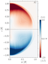 |
Fig. 4. Azimuthally averaged normalised kinetic helicity, |

3.1.3. Convective energy transport
The luminosities corresponding to radiative, enthalpy, kinetic energy, cooling, and heating fluxes according to Eqs. (31)–(36) of Käpylä (2021) are shown in Fig. 5 for run C4. The enthalpy and kinetic energy fluxes dominate almost everywhere, except near the surface where the cooling becomes important. This is similar to the results of Brown et al. (2020) and to the rotating runs of Käpylä (2021). The total flux reaches somewhat less than 90% of the luminosity from the heating near the surface. A possible reason for this discrepancy is a non-negligible contribution from the SGS flux.
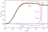 |
Fig. 5. Luminosity profiles of kinetic energy (purple), cooling (blue), heating (orange), and enthalpy (red) fluxes of run C4. |
3.2. Dynamo variation
As shown in Table 1, the main differences between the simulations are the input parameters PrM and the rotation rate. In this subsection we present the effects of varying these parameters on the large-scale magnetic field.
3.2.1. Dependence on rotation
We explored simulations with fixed PrM and varying Prot with values between 43 and 90 days. These values were determined using the conversion method outlined in Appendix A of Käpylä (2021). In order to compare the large-scale magnetic field at the three rotation rates used here, we chose runs with comparable magnetic Reynolds numbers and different rotation rates.
Three representative runs with ReM < 100 from each set are A6 with ReM = 75, B1 with ReM = 84, and C3 with ReM = 67. Run A6 shows cycles in the azimuthally averaged toroidal magnetic field,  , as shown in the middle top panel of Fig. 6. The cycles were computed using the empirical mode decomposition with the libeemd library (Luukko et al. 2016), as in Käpylä (2022). To determine the periods we used
  , from the range −60° < θ < 60°. The cycle was determined by taking the mode with the largest energy, and counting the period from the zero crossings of that mode.
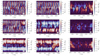 |
Fig. 6. Azimuthally averaged toroidal magnetic field near the surface of the star as a function of time. The name of the simulation is indicated at the bottom right of each panel. |
The left middle panel of Fig. 6 shows  for run B1, which also exhibits cycles. The reversals are periodic for most of the run, and this run also shows longer term modulation in the northern hemisphere towards the end of the run. The left bottom panel of Fig. 6 is for run C3. Unlike the runs just mentioned, C3 does not exhibit cyclic reversals. However, it does reveal the presence of a dipolar field, with a positive (negative) polarity in the northern (southern) hemisphere. At similar values of magnetic Reynolds number, the third column of Table 1 indicates a slight reduction in Brms at lower rotation rates.
Three representative runs with higher magnetic Reynolds number (ReM ≈ 300) and different rotation rates are A15 with ReM = 300, B3 with ReM = 315, and C4 with ReM = 337. The right top panel of Fig. 6 shows  of run A15. This run has irregular reversals with the field mainly distributed from mid-latitudes (±45°) to the equator. Near the poles the field is quasi-stationary. The middle centre panel of Fig. 6 is for B3, where a dipole with a few random reversals is visible with a predominantly negative (positive) polarity at the northern (southern) hemisphere. The azimuthally averaged toroidal magnetic field of C4 is shown in the centre bottom panel of Fig. 6, where a predominantly positive (negative) polarity. Mollweide projections of the radial magnetic field at the surface of runs A15, B3, and C4 are shown in Fig. 7, where the field is less intense for the runs with lower rotation. In this sense, the Brms decreases with decreasing rotation rate from A15 to B3, while B3 and C4 have similar values. We find that in general the saturation level of the magnetic field increases with ReM. This behaviour is likely related to the presence of a small-scale dynamo that produces magnetic fields at spatial scales that are of the same order of magnitude as that of the turbulence. While this was not the focus of our current study, it remains an important area for future research.
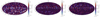 |
Fig. 7. Mollweide projection of the radial magnetic field Br for runs A15, B3 and C4 with ReM ≈ 300 and different rotation rates. |
In Fig. 8 we show the ratio of the rotation period to cycle period as a function of the global Coriolis number. We find that Prot/Pcyc ∝ Coβ with β = −1.30 ± 0.26. When considering the data points on the right of the figure, we find that β = −2.98 ± 1.13. The uncertainty in the slope indicates that we need to take these results with caution. Nevertheless, earlier studies have also found β < 0 (e.g., Strugarek et al. 2017, 2018; Warnecke 2018; Viviani et al. 2018) with global simulations of solar-like stars. Even when the domain of these simulations differs from the one presented here, the similarity in the relationship between the cycle period and the Coriolis number implies a likeness in the dynamo processes of solar-like and fully convective stars. Nevertheless, the negative slope found here differs from the positive slopes for the inactive and active branches from observations (Brandenburg et al. 1998, 2017). However, some simulations show β ≳ 0 (Guerrero et al. 2019; Käpylä 2022), but the cause of this behaviour is currently unclear.
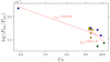 |
Fig. 8. Rotation period normalised to the cycle period as a function of the global Coriolis number. The green circles are for ReM ∼ 100, blue for 70 < ReM < 85, and yellow for ReM ≤ 55. |
3.2.2. Dependence on magnetic Reynolds and Prandtl numbers
Magnetic Prandtl numbers from 0.1 to 10 were used in the simulations. For all the current runs, the magnetic field is predominantly axisymmetric. When converted to physical units, the azimuthally averaged toroidal magnetic field reaches strengths ranging from 10 to 16 kG in our models. These values are higher than those of the reported observations which are up to a few kG (e.g., Kochukhov 2021). Set A has cycles for PrM ≤ 2 with periods ranging from 309 to 471 free-fall times, which correspond to 6.3–9.6 yr, when considering the same time conversion factor used by Käpylä (2021). Run B1 also shows cycles with a period of 274 free-fall times. Table 3 lists the values of ν, η, the cycle periods (if applicable) together with the corresponding standard deviation for all the simulations presented here. We found that the calculated length of the cycle periods of the runs of set A has a very slight increase when increasing the magnetic Reynolds number as  with α = 0.25 ± 0.14. Additionally, when considering the runs with similar ReM and different PrM, we found that the cycle period is virtually independent of PrM in the parameter regime explored here.
Diffusivities, cycles, and averaged energy densities.
The azimuthally averaged toroidal magnetic field  is shown in Fig. 6 for a set of representative runs. The top panels are for three runs of set A, which have the same rotation period and increasing ReM from left to right. The top left panel is for run A1 with ReM = 55, with Pcyc = 320 ± 10 free-fall times. The top centre panel is for run A6 with ReM = 75 and Pcyc = 326 ± 11 free-fall times. In these cases the field is distributed in latitudes |θ|≲80°. Simulations with higher values of PrM and ReM, such as run A15 with ReM = 300, result in the loss of cycles and the emergence of irregular solutions. Similar irregularities of dynamo solutions have previously been observed in simulations with high ReM (e.g., Käpylä et al. 2017), but the exact mechanism is still unknown. In this case the field is distributed at latitudes |θ|≲50 and also exhibits quasi-stationary solutions near the poles.
The polarity of the field changes from the surface to r = 0.5 R. Figure 9 shows  at r = 0.5 R for runs A1 and A15. In simulations with cycles, such as A1, the cycles are visible throughout the convection zone. However, for runs with higher magnetic Prandtl number (PrM > 2), such as A15, the azimuthally averaged toroidal magnetic field changes with depth and shows less clear magnetic structures in the deeper layers.
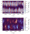 |
Fig. 9. Azimutally averaged toroidal magnetic field at r = 0.5 for simulations A1 (top) and A15 (bottom) with ReM = 55 and ReM = 300, respectively. |
The second row of Fig. 6 shows three runs from set B that have the same rotation rate and increasing ReM. The left panel is for run B1 with ReM = 84, which exhibits a cycle with Pcyc = 274 ± 38 free-fall times, as well as longer reversals or disappearing cycles towards the end of the run. In this run the field is distributed at latitudes |θ|≲80°. The centre panel is for run B3 with ReM = 315, which exhibits an irregular solution with few polarity reversals and predominantly quasi-static fields. In this case the field spans slightly less latitudinally, distributed at latitudes |θ|≲75°. The right centre panel of Fig. 6 shows run B5, which has the highest PrM and ReM in this set with PrM = 10 and ReM = 1360. The field is more concentrated towards the equator (at latitudes |θ|≲50°) with seemingly irregular reversals. Similar to run A15, B5 also has a quasi-stationary solution near the poles. The third row of Fig. 6 are for runs of set C, which have the slowest rotation in the present work, with increasing ReM from left to right. Runs C3 with ReM = 67 and C4 with ReM = 337 show a predominantly quasi-static dipolar field, which spans latitudes |θ|≲75°. A similar dipolar field was reported by Moutou et al. (2017) for the fully convective and slow-rotating M dwarf GJ 1289. However, in our models the toroidal magnetic energy is dominant (see Table 3), whereas the large-scale magnetic field of GJ 1289 is purely poloidal. Run C6 with ReM = 1419 has a field concentrated near the equator and the large-scale structures are less clear than in C3 and C4.
The radial magnetic field, Br, also varies as a function of ReM. Mollweide projections of the radial magnetic field for runs B1, B2, and B5, with increasing ReM from left to right are presented in Fig. 10. The main differences here are the structure and maximum values of the magnetic field strength. The size of the structures in runs B1 and B2 are similar, but the strength of the field is slightly higher in B2. Run B5 has smaller field structures than in the previous cases, and the magnetic field strength is higher.
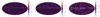 |
Fig. 10. Mollweide projection of the radial magnetic field Br for runs with the same rotation rate and different ReM, B1 with ReM = 84, B2 with ReM = 168, and B5 with ReM = 1360. |
Table 3 lists the energy densities of the simulations. The total magnetic energy Emag is a significant fraction of the kinetic energy density in all of the runs with dynamos, sometimes also exceeding it. One may expect that Emag grows with increasing ReM (PrM), as found in other works (e.g., Käpylä et al. 2017). In this regard, there is no discernible trend in the simulations shown here in terms of the variation of Emag. Since the kinetic energy density, Ekin, decreases with increasing PrM the ratio Emag/Ekin grows. The decrease in the kinetic energy can be explained because at large PrM it is converted into magnetic energy more efficiently.
At low PrM the kinematic exponentially growing regime lasts longer than in the simulations with high PrM. Figure 11 shows the evolution of Emag and Ekin in the kinematic and saturated regimes for runs A4 and A16. The kinematic regime of simulation A4 lasted about ten times longer than the kinematic regime of run A16. It can be seen in simulation A4 that Emag is amplified by six orders of magnitude. In the saturated regime both energies are comparable, such that Ekin is about 1.5 times Emag. However, in simulation A16 the kinetic energy density is slightly reduced, while the magnetic energy density is increased by a factor of roughly 1.8. The PrM at which Emag overcomes Ekin occurs at PrM > 1 for sets A and B, and at PrM > 2 for set C. A similar behaviour of the kinetic and magnetic energy densities was reported by Browning (2008) for simulations of fully convective stars. In run Cm2 of that work with PrM = 5, Emag/Ekin ≤ 1, while Cm with PrM = 8 has Emag/Ekin = 1.2.
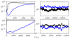 |
Fig. 11. Time evolution of the kinetic (black) and magnetic (blue) energy densities in the kinematic (left) and saturated (right) regimes for simulations A16 with PrM = 10 (top) and A4 PrM = 0.5 (bottom). The energies are normalised by Ekin. |
Table 3 also includes the energy densities of mean toroidal ( ) and poloidal (
 ) magnetic fields (see Cols. 8 and 9). The mean toroidal
  accounts for up to 30% of total magnetic energy density and, in general, diminishes as ReM increases.
  is less than 10% of Emag for almost all simulations. In general, the ratio of the energy of the mean field to total energy decreases for high magnetic Reynolds numbers. Figure 12 shows the saturation level of the mean field as a function of ReM for subsets of simulations from sets A and B. We do not find a clear trend in the saturation level of the mean energy as a function of the magnetic Reynolds number. A decrease in the mean energy with the inverse magnetic Reynolds number is usually associated with catastrophic quenching (e.g., Cattaneo & Vainshtein 1991; Brandenburg 2001). It can be interpreted as an outcome of magnetic helicity conservation, which becomes important as ReM grows (e.g., Brandenburg & Subramanian 2005). Nevertheless, the boundary conditions in our simulations do allow magnetic helicity fluxes.
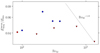 |
Fig. 12. Mean magnetic energy normalised by kinetic energy as a function of the magnetic Reynolds number. The blue markers are for the last four simulations of set A; the red markers are for the simulations of set B. Circles (triangles) are for runs with 2003 (5763) of resolution. The dotted line corresponds to a power law that shows what a decrease in mean energy with the inverse magnetic Reynolds number might look like. |
Furthermore, the kinetic energy density of the differential rotation,  , and meridional circulation,
  , are given in Table 3. For simulations with a dynamo
  decreases at higher ReM, while for simulations A8 and A12 with no dynamo
  is significantly higher. More specifically, the runs without a dynamo in set A exhibit roughly five times higher
  than runs with a dynamo in the same set. This indicates magnetic quenching of differential rotation. In all of the simulations discussed here,
  is around 1–3% of Ekin, with the exception of C2, where
  .
.
4. Summary and conclusions
We have performed a large number of simulations of fully convective M dwarfs using the star-in-a-box set-up presented in Käpylä (2021). We used the stellar parameters for an M5 dwarf with 0.21 M⊙ at three rotation rates corresponding to Prot = 43, 61, and 90 days, and varied the magnetic Prandtl number from 0.1 to 10. Our simulations explore the intermediate to slowly rotating regime. Consistent with previous work by Käpylä (2021), we find solar-like differential rotation in the simulations presented here.
We found different solutions for the large-scale magnetic field depending on the rotation period and the magnetic Prandtl number, which in our models fixes the magnetic Reynolds number. For the simulations with  (set A) and ReM ≤ 105, the large-scale magnetic field is cyclic, with Pcyc ranging from 309 to 471 free-fall times. In this set we found a slight increase in the length of the cycle period with increasing ReM. For larger ReM no clear cycles are found, and instead the behaviour of the magnetic field and its reversals become irregular. For the simulations with
  (set B) we found cycles for run B1 with ReM = 84, while for higher values of ReM the reversals are less regular, and instead a quasi-static configuration is found. For the highest ReM the solutions become irregular. For the case with the lowest rotation rate (
 ) the field is mainly dipolar for ReM ≤ 750. At higher magnetic Reynolds numbers the magnetic field is predominantly irregular and concentrated at mid-latitudes, with quasi-stationary fields near the poles. We note that in the three sets the large-scale field is irregular and concentrated near the equator for the highest PrM (ReM). Additionally, the rms velocity increases for decreasing rotation for comparable ReM. We also note that for a few of the simulations, particularly A8, A12, and C2, no dynamo was found because ReM was below the critical value to drive a large-scale dynamo.
Furthermore, the ratio Prot/Pcyc decreases with the Coriolis number, similar to the simulations of solar-like stars by Strugarek et al. (2017, 2018), Warnecke (2018), and Viviani et al. (2018). Our results confirm the important role of rotation and dimensionless parameters such as ReM and PrM in determining the properties of fully convective dynamos. Depending on the parameters, the magnetic field can show a clear cyclic behaviour with the cycle period influenced by the rotation rate and dimensionless parameters such as ReM and PrM. The large-scale magnetic field shows cycles for low and modest values of ReM, but the cycles are lost for highest magnetic Reynolds numbers where irregular or quasi-static fields dominate. A similar loss of cyclic solutions was reported by Käpylä et al. (2017) who also increased PrM to increase ReM. Whether the behaviour of the dynamo changes if ReM is fixed and PrM is lowered is yet an open question. This is also closer to the parameter regime of late-type stars where PrM ≪ 1 and ReM ≫ 1, but this parameter regime is extremely challenging numerically.
A very tentative comparison can be pursued with the Proxima Centauri system, where Klein et al. (2021) inferred a seven-year activity cycle. In principle, the activity cycle inferred in our simulations is in the range from five to nine years, and is thus consistent with the observed data. We note that this comparison is preliminary; even though the rotation rate we adopt here is similar, the magnetic Prandtl number is likely to be different, and even larger differences are expected when comparing the magnetic Reynolds number of the star with that of our simulations. It is well known that the solutions for the magnetic field depend on these parameters, and thus leads to uncertainty in the possible interpretation. It is nevertheless encouraging that the behaviour found in the simulations is quite similar.
Overall, the study presented here, to our knowledge, consists of the largest exploration of the parameter space for dynamo models of fully convective M dwarfs. Uncertainties remain, for instance regarding the role of the magnetic Reynolds number, which will still be much larger in realistic systems. While a clear signature of a small-scale dynamo is not found in our simulations, the expectation is that small-scale dynamos are present at larger magnetic Reynolds numbers, and interact with the large-scale dynamo, thereby changing the solution.
Acknowledgments
C.A.O.R., D.R.G.S. and J.P.H. thank for funding via Fondecyt Regular (project code 1201280). C.A.O.R., D.R.G.S. and R.E.M. gratefully acknowledge support by the ANID BASAL projects ACE210002 and FB210003. D.R.G.S. and R.E.M. gratefully acknowledge support by the FONDECYT Regular 1190621. D.R.G.S. thanks for funding via the Alexander von Humboldt – Foundation, Bonn, Germany. P.J.K. acknowledges finantial support from DFG Heisenberg programme grant No. KA 4825/4-1. F.H.N. acknowledges financial support by the DAAD (Deutscher Akademischer Austauschdienst; code 91723643). The simulations were made using the Kultrun cluster hosted at the Departamento de Astronomía, Universidad de Concepción, and on HLRN-IV under project grant hhp00052.
References
- Augustson, K. C., Brun, A. S., & Toomre, J. 2019, ApJ, 876, 83 [Google Scholar]
- Bice, C. P., & Toomre, J. 2020, ApJ, 893, 107 [NASA ADS] [CrossRef] [Google Scholar]
- Brandenburg, A. 2001, ApJ, 550, 824 [Google Scholar]
- Brandenburg, A., & Subramanian, K. 2005, Phys. Rep., 417, 1 [NASA ADS] [CrossRef] [Google Scholar]
- Brandenburg, A., Saar, S. H., & Turpin, C. R. 1998, ApJ, 498, L51 [NASA ADS] [CrossRef] [Google Scholar]
- Brandenburg, A., Mathur, S., & Metcalfe, T. S. 2017, ApJ, 845, 79 [NASA ADS] [CrossRef] [Google Scholar]
- Brown, B. P., Oishi, J. S., Vasil, G. M., Lecoanet, D., & Burns, K. J. 2020, ApJ, 902, L3 [NASA ADS] [CrossRef] [Google Scholar]
- Browning, M. K. 2008, ApJ, 676, 1262 [Google Scholar]
- Brun, A. S., & Browning, M. K. 2017, Liv. Rev. Sol. Phys., 14, 4 [Google Scholar]
- Brun, A. S., Miesch, M. S., & Toomre, J. 2004, ApJ, 614, 1073 [Google Scholar]
- Cattaneo, F., & Vainshtein, S. I. 1991, ApJ, 376, L21 [NASA ADS] [CrossRef] [Google Scholar]
- Chabrier, G., & Baraffe, I. 1997, A&A, 327, 1039 [NASA ADS] [Google Scholar]
- Chandrasekhar, S. 1961, Hydrodynamic and Hydromagnetic Stability (Oxford: Clarendon) [Google Scholar]
- Dobler, W., Stix, M., & Brandenburg, A. 2006, ApJ, 638, 336 [NASA ADS] [CrossRef] [Google Scholar]
- Featherstone, N. A., & Hindman, B. W. 2016, ApJ, 830, L15 [Google Scholar]
- Guerrero, G., Zaire, B., Smolarkiewicz, P. K., et al. 2019, ApJ, 880, 6 [NASA ADS] [CrossRef] [Google Scholar]
- Hotta, H., Kusano, K., & Shimada, R. 2022, ApJ, 933, 199 [NASA ADS] [CrossRef] [Google Scholar]
- Jermyn, A. S., Anders, E. H., Lecoanet, D., & Cantiello, M. 2022, ApJS, 262, 19 [NASA ADS] [CrossRef] [Google Scholar]
- Käpylä, P. J. 2021, A&A, 651, A66 [Google Scholar]
- Käpylä, P. J. 2022, ApJ, 931, L17 [CrossRef] [Google Scholar]
- Käpylä, P. J. 2023, A&A, 669, A98 [NASA ADS] [CrossRef] [EDP Sciences] [Google Scholar]
- Käpylä, P. J., Käpylä, M., Olspert, N., Warnecke, J., & Brandenburg, A. 2017, A&A, 599, A4 [NASA ADS] [CrossRef] [EDP Sciences] [Google Scholar]
- Käpylä, P. J., Käpylä, M. J., & Brandenburg, A. 2018, Astron. Nachr., 339, 127 [CrossRef] [Google Scholar]
- Käpylä, P. J., Gent, F. A., Olspert, N., Käpylä, M. J., & Brandenburg, A. 2020, Geophys. Astrophys. Fluid Dyn., 114, 8 [CrossRef] [Google Scholar]
- Klein, B., Donati, J.-F., Hébrard, É. M., et al. 2021, MNRAS, 500, 1844 [Google Scholar]
- Kochukhov, O. 2021, A&A Rev., 29, 1 [NASA ADS] [CrossRef] [Google Scholar]
- Luukko, P. J., Helske, J., & Räsänen, E. 2016, Comput. Stat., 31, 545 [CrossRef] [Google Scholar]
- Morin, J., Donati, J.-F., Petit, P., et al. 2010, MNRAS, 407, 2269 [Google Scholar]
- Moutou, C., Hébrard, E., Morin, J., et al. 2017, MNRAS, 472, 4563 [NASA ADS] [CrossRef] [Google Scholar]
- Navarrete, F. H., Schleicher, D. R., Käpylä, P. J., Ortiz-Rodríguez, C. A., & Banerjee, R. 2022, A&A, 667, A164 [NASA ADS] [CrossRef] [EDP Sciences] [Google Scholar]
- Newton, E. R., Irwin, J., Charbonneau, D., et al. 2017, ApJ, 834, 85 [Google Scholar]
- Parker, E. N. 1955, ApJ, 122, 293 [Google Scholar]
- Brandenburg, A. 2021, J. Open Source Softw., 6, 2807 [CrossRef] [Google Scholar]
- Reiners, A., Shulyak, D., Käpylä, P. J., et al. 2022, A&A, 662, A41 [NASA ADS] [CrossRef] [EDP Sciences] [Google Scholar]
- Rogachevskii, I., & Kleeorin, N. 2015, J. Plasma Phys., 81, 395810504 [Google Scholar]
- Saar, S. H., & Linsky, J. L. 1985, ApJ, 299, L47 [Google Scholar]
- Schekochihin, A. A., Iskakov, A. B., Cowley, S. C., et al. 2007, New J. Phys., 9, 300 [Google Scholar]
- Schrinner, M., Petitdemange, L., & Dormy, E. 2012, ApJ, 752, 121 [NASA ADS] [CrossRef] [Google Scholar]
- Steenbeck, M., Krause, F., & Rädler, K.-H. 1966, Z. Naturf. A, 21, 369 [NASA ADS] [CrossRef] [Google Scholar]
- Strugarek, A., Beaudoin, P., Charbonneau, P., Brun, A., & do Nascimento, J.-D., Jr. 2017, Science, 357, 185 [NASA ADS] [CrossRef] [Google Scholar]
- Strugarek, A., Beaudoin, P., Charbonneau, P., & Brun, A. 2018, ApJ, 863, 35 [NASA ADS] [CrossRef] [Google Scholar]
- Viviani, M., Warnecke, J., Käpylä, M. J., et al. 2018, A&A, 616, A160 [NASA ADS] [CrossRef] [EDP Sciences] [Google Scholar]
- Warnecke, J. 2018, A&A, 616, A72 [NASA ADS] [CrossRef] [EDP Sciences] [Google Scholar]
- Wright, N. J., & Drake, J. J. 2016, Nature, 535, 526 [Google Scholar]
- Wright, N. J., Newton, E. R., Williams, P. K., Drake, J. J., & Yadav, R. K. 2018, MNRAS, 479, 2351 [NASA ADS] [CrossRef] [Google Scholar]
- Yadav, R. K., Christensen, U. R., Morin, J., et al. 2015, ApJ, 813, L31 [Google Scholar]
- Yadav, R. K., Christensen, U. R., Wolk, S. J., & Poppenhaeger, K. 2016, ApJ, 833, L28 [Google Scholar]
- Yoshimura, H. 1975, ApJ, 201, 740 [Google Scholar]
All Tables
All Figures
|
Fig. 1. Amplitude of radial differential rotation as a function of magnetic Reynolds number for simulations of sets A (circles), B (squares), and C (triangles). Cyan and red is for simulations with dynamo and without dynamo, respectively. |
| In the text | |
|
Fig. 2. Normalised time-averaged mean angular velocity |
| In the text | |
|
Fig. 3. Normalised convective power as a function of ℓ for simulations A10, A13, A16, B2, B3, B5, C2, C3, C4, and C6. |
| In the text | |
|
Fig. 4. Azimuthally averaged normalised kinetic helicity, |
| In the text | |
|
Fig. 5. Luminosity profiles of kinetic energy (purple), cooling (blue), heating (orange), and enthalpy (red) fluxes of run C4. |
| In the text | |
|
Fig. 6. Azimuthally averaged toroidal magnetic field near the surface of the star as a function of time. The name of the simulation is indicated at the bottom right of each panel. |
| In the text | |
|
Fig. 7. Mollweide projection of the radial magnetic field Br for runs A15, B3 and C4 with ReM ≈ 300 and different rotation rates. |
| In the text | |
|
Fig. 8. Rotation period normalised to the cycle period as a function of the global Coriolis number. The green circles are for ReM ∼ 100, blue for 70 < ReM < 85, and yellow for ReM ≤ 55. |
| In the text | |
|
Fig. 9. Azimutally averaged toroidal magnetic field at r = 0.5 for simulations A1 (top) and A15 (bottom) with ReM = 55 and ReM = 300, respectively. |
| In the text | |
|
Fig. 10. Mollweide projection of the radial magnetic field Br for runs with the same rotation rate and different ReM, B1 with ReM = 84, B2 with ReM = 168, and B5 with ReM = 1360. |
| In the text | |
|
Fig. 11. Time evolution of the kinetic (black) and magnetic (blue) energy densities in the kinematic (left) and saturated (right) regimes for simulations A16 with PrM = 10 (top) and A4 PrM = 0.5 (bottom). The energies are normalised by Ekin. |
| In the text | |
|
Fig. 12. Mean magnetic energy normalised by kinetic energy as a function of the magnetic Reynolds number. The blue markers are for the last four simulations of set A; the red markers are for the simulations of set B. Circles (triangles) are for runs with 2003 (5763) of resolution. The dotted line corresponds to a power law that shows what a decrease in mean energy with the inverse magnetic Reynolds number might look like. |
| In the text | |
Current usage metrics show cumulative count of Article Views (full-text article views including HTML views, PDF and ePub downloads, according to the available data) and Abstracts Views on Vision4Press platform.
Data correspond to usage on the plateform after 2015. The current usage metrics is available 48-96 hours after online publication and is updated daily on week days.
Initial download of the metrics may take a while.