| Issue |
A&A
Volume 678, October 2023
|
|
|---|---|---|
| Article Number | A9 | |
| Number of page(s) | 8 | |
| Section | Astrophysical processes | |
| DOI | https://doi.org/10.1051/0004-6361/202346768 | |
| Published online | 26 September 2023 | |
Effects of the centrifugal force in stellar dynamo simulations
1
Hamburger Sternwarte, Universität Hamburg, Gojenbergsweg 112, 21029 Hamburg, Germany
e-mail: This email address is being protected from spambots. You need JavaScript enabled to view it.
2
Leibniz-Institut für Sonnenphysik (KIS), Schöneckstr. 6, 79104 Freiburg, Germany
3
Institut für Astrophysik und Geophysik, Georg-August-Universität Göttingen, Friedrich-Hund-Platz 1, 37077 Göttingen, Germany
4
Departamento de Astronomía, Facultad de Ciencias Físicas y Matemáticas, Universidad de Concepción, Av. Estebar Iturra s/n Barrio Universitario, Casilla 160, Chile
Received:
28
April
2023
Accepted:
3
July
2023
Abstract
Context. The centrifugal force is often omitted from simulations of stellar convection either for numerical reasons or because it is assumed to be weak compared to the gravitational force. However, the centrifugal force might be an important factor in rapidly rotating stars, such as solar analogs, due to its Ω2 scaling, where Ω is the rotation rate of the star.
Aims. We study the effects of the centrifugal force in a set of 21 semi-global stellar dynamo simulations with varying rotation rates. Included in the set are three control runs aimed at distinguishing the effects of the centrifugal force from the nonlinear evolution of the solutions.
Methods. We solved the 3D magnetohydrodynamic equations with the PENCIL CODE in a solar-like convective zone in a spherical wedge setup with a 2π azimuthal extent. The rotation rate and the amplitude of the centrifugal force were varied. We decomposed the magnetic field into spherical harmonics and studied the migration of azimuthal dynamo waves (ADWs), the energy of different large-scale magnetic modes, and differential rotation.
Results. In the regime with the lowest rotation rates, Ω = 5 − 10 Ω⊙, where Ω⊙ is the rotation rate of the Sun, we see no marked changes in either the differential rotation or the magnetic field properties. For intermediate rotation, Ω = 20 − 25 Ω⊙, we identify an increase in the differential rotation as a function of centrifugal force. The axisymmetric magnetic energy tends to decrease with centrifugal force, while the non-axisymmetric one increases. The ADWs are also affected, especially in the propagation direction. In the most rapidly rotating set with Ω = 30 Ω⊙, these changes are more pronounced, and in one case the propagation direction of the ADW changes from prograde to retrograde. The control runs suggest that the results are a consequence of the centrifugal force and not due to the details of the initial conditions or the history of the run.
Conclusions. We find that the differential rotation and properties of the ADWs only change as a function of the centrifugal force when rotation is rapid enough.
Key words: turbulence / convection / dynamo / stars: magnetic field
© The Authors 2023
 Open Access article, published by EDP Sciences, under the terms of the Creative Commons Attribution License (https://creativecommons.org/licenses/by/4.0), which permits unrestricted use, distribution, and reproduction in any medium, provided the original work is properly cited.
This article is published in open access under the Subscribe to Open model. This email address is being protected from spambots. You need JavaScript enabled to view it. to support open access publication.
1. Introduction
Simulations of stellar convection, usually aimed at explaining solar phenomena, often omit the centrifugal force. This is due to the assumption that its amplitude is small due to the relatively slow rotation of the Sun. Earlier in its history, however, the Sun must have been rotating much more rapidly because, in general, stars are born with larger angular momenta that are slowly reduced via magnetic braking (Skumanich 1972; Matt et al. 2012). Therefore, the influence of the centrifugal force is expected to be more important at earlier stages because its amplitude increases as the square of the rotation rate. To study these phases of rapid ration in the solar context, such as magnetic field evolution, one has to study young solar analogs at earlier phases that are rotating much faster than the Sun (e.g., Lehtinen et al. 2016). This allows us to study the evolution of the Sun up to the present, given that outflows that are produced by magnetic braking do not significantly affect the structure of the star, only the rotation rate.
Observations by Lehtinen et al. (2016) of magnetic fields of solar analogs reveal that they are active and show a characteristic split between the axisymmetric and non-axisymmetric spot distributions. These authors also estimate that, among solar-like stars with non-axisymmetric spot distribution, the active longitude periods are shorter than the rotation period of the star. One plausible explanation is the presence of azimuthal dynamo waves (ADWs). These waves propagate in the rotating frame of reference of the star either in prograde or retrograde fashion with a uniform frequency irrespective of the underlying fluid motions. Such solutions were first discovered in linear mean-field dynamo models (e.g., Krause & Rädler 1980). To explain their observations, Lehtinen et al. (2016) argue that the propagation of the ADWs must be prograde.
V530 Per is an extreme case of a rapidly rotating Sun-like star with an estimated rotation period of 0.32 days (Cang et al. 2020), which corresponds to about 75 Ω⊙, where Ω⊙ is the rotation rate of the Sun. This makes the gravitational force at its surface only 9.5 times larger than the centrifugal force. In comparison, in the Sun this ratio is 5.3 × 10⁴. There are also clear differences between the magnetic field of V530 Per and the Sun. For example, Cang et al. (2020) also find that the magnetic field distribution of V530 Per is asymmetric with respect to the equator. It is characterized by a stronger magnetic field near the north pole, with a peak field strength of 1 kG. It is as yet unclear why similar stars have different field strengths and symmetries, but there are indications that rotation may play an important role in the magnetic activity of Sun-like stars (Lehtinen et al. 2016) as well as low-mass stars (e.g., Reiners et al. 2022).
Such rapid rotation is commonly found in close binaries if tidal locking is assumed. For example, V471 Tau is a post-common-envelope binary in which the secondary is a main-sequence solar-like star with a mass of 0.93 M⊙, a radius of 0.96 R⊙, and a binary period of about 0.5 days (e.g., Völschow et al. 2016). If tidal locking is assumed, this gives a ratio of gravitation to centrifugal forces of about 22. Interestingly, Zaire et al. (2022) analyzed the magnetic activity of the K2 star in V471 Tau and find that the magnetic field is also dominated by a concentration on one hemisphere. They also find that the spot coverage and brightness map, derived from Zeeman-Doppler imaging, do not follow the magnetic activity cycle inferred from Hα variability. This suggests that it might be inappropriate to use spot coverage to study magnetic cycles in rapidly rotating stars (Zaire et al. 2022).
Simulations of stellar dynamos often produce ADWs whose characteristics change with the rotation rate and the physics involved. Cole et al. (2014) studied the propagation properties of ADWs in a set of three runs with moderate rotation rates of up to 6.7 times the solar value with 3D magnetohydrodynamic simulations. They find that the waves have a rotation rate that is slower than that of the gas, that is, they are retrograde. The magnetic structure in the ADW propagates like a rigid body, and therefore such motion cannot be explained by advection by the fluid in a differentially rotating convection zone. This result was later confirmed by Viviani et al. (2018) with a larger set of runs. Most of their runs show retrograde ADWs independently of the rotation rate, but in some cases standing or prograde waves appeared. Recently, Viviani & Käpylä (2021) presented a set of four runs with moderate rotation rates where the usual prescribed radial dependence of the radiative heat conductivity was replaced by the more realistic Kramers opacity law (Brandenburg et al. 2000; Käpylä et al. 2017). This suggests that using this heat conductivity might affect the direction of the propagation of ADWs indirectly by affecting the flow through the pressure gradient and/or dissipation. However, it might come with the cost of pushing the transition point of differential rotation profiles of simulations from anti-solar profiles to solar-like profiles to even larger Coriolis numbers (Viviani & Käpylä 2021).
Navarrete et al. (2022b) explored the effect of the centrifugal force in the context of changes in the internal structure of the stars, with the aim to check whether the resulting changes are sufficient to explain the observed eclipsing time variations in post-common-envelope binaries, as proposed in the Applegate scenario (Applegate 1992). In this paper we study the effects of centrifugal force in semi-global dynamo simulations further. We focus on differential rotation, magnetic energy, and ADW propagation. In Sect. 2 we present the model and the implementation of the centrifugal force. Section 3 presents the results, and our conclusions are drawn in Sect. 4.
2. Model
We solved the fully compressible magnetohydrodynamic equations in a spherical grid with coordinates (r, Θ, ϕ), where 0.7R ≤ r ≤ R is radius and R is the radius of the star, π/12 ≤ Θ ≤ 11π/12 is the colatitude, and 0 ≤ ϕ < 2π is the longitude. The model is the same as in Käpylä et al. (2013) and Navarrete et al. (2020, 2022a). The equations adopt the following forms:
 (1)
(1)
 (2)
(2)
 (3)
(3)
![Mathematical equation: $$ \begin{aligned} T\frac{\mathrm{D}s}{\mathrm{D}t}&= \frac{1}{\rho }\left[\eta \mu _0{\boldsymbol{J}}^2 - {\boldsymbol{\nabla }}{\boldsymbol{\cdot }}({\boldsymbol{F}}^\mathrm{rad} + {\boldsymbol{F}}^\mathrm{SGS})\right] + 2\nu {\boldsymbol{S}}^2, \end{aligned} $$](/articles/aa/full_html/2023/10/aa46768-23/aa46768-23-eq4.gif) (4)
(4)
where A is the magnetic vector potential, B = ∇ × A is the magnetic field, u is the velocity field, η is the magnetic diffusivity, μ0 is the vacuum permeability, t is the time, J = ∇ × B/μ0 is the electric current density, ρ is the mass density, p is the pressure, ν is the viscosity,
 (5)
(5)
is the rate-of-strain tensor, where semicolons denote covariant differentiation, T is the temperature, and s is the specific entropy. Furthermore, Frad = −K∇T is the radiative flux, which we modeled with the diffusion approximation, where K = K(r) has a fixed spatial profile (see Sect. 2.1 in Käpylä et al. 2014). We also investigated the effects of Kramers opacity in some runs (see Sect. 3.3). We did this by replacing the radiative heat conductivity, K, in the radiative flux term Frad = −K∇T with
 (6)
(6)
where a = 1 and b = −7/2 correspond to the Kramers opacity law (Brandenburg et al. 2000). Here, K0 is a constant that depends on natural constants and, in simulations, on the luminosity of the model (Viviani & Käpylä 2021). The FSGS = −χSGSρT∇s is a sub-grid scale flux that we implemented to smooth grid-scale fluctuations that would otherwise make the system unstable. Here, χSGS is the sub-grid scale entropy diffusivity, and it varies smoothly from 0 at r/R = 0.7 to 0.4ν at r/R = 0.72; it then smoothly increases by a factor of 12.5 at r/R = 0.98, above which it is constant. The first three terms on the right-hand side of Eq. (4),
 (7)
(7)
 (8)
(8)
 (9)
(9)
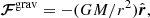
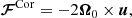
are the gravitational, Coriolis, and centrifugal forces.
2.1. Boundary and initial conditions
The magnetic field follows a perfect conductor condition at the bottom of the convective zone and is radial at the surface. The temperature gradient was kept fixed at the bottom, whereas at the top we applied a black-body condition. For the entropy and density, we assumed a vanishing first derivative at both latitudinal boundaries. The latitudinal boundaries are stress-free and perfectly conducting. The initial state is isentropic. Perturbations were introduced by initializing the magnetic and velocity fields with low-amplitude Gaussian white noise.
2.2. Centrifugal force
The parameter cf in Eq. (9) was introduced by Käpylä et al. (2020) and controls the strength of the centrifugal force. A cf value of 1 corresponds to the unaltered centrifugal force amplitude, and cf = 0 implies no centrifugal force. It is defined as
 (10)
(10)
with  being the unaltered magnitude of the centrifugal force. The necessity of controlling the centrifugal force is due to the enhanced luminosity and rotation rate in simulations of compressible stellar (magneto-)convection. Similarly to Käpylä et al. (2020), each run was initialized with cf = 0 and was increased in small incremental steps after the saturated regime is reached.
To get a sense of how strong the centrifugal force is in our simulations, we computed the ratio of centrifugal to gravitational forces in the simulations as well as in a real Sun-like star with the same rotation rate. We defined the ratio between the two as
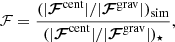 (11)
(11)
where the subscripts ⋆ denote the real star and “sim” the simulations. These values are shown in the last column of Table 1. By using a value as low as cf = 10−4, our simulations are influenced by the centrifugal force just below the value that the equivalent star with the same rotation rate and radius would have, and the simulations that have the strongest centrifugal force have ℱ = 87.
Summary of the simulation parameters.
3. Results
We ran a total of 21 simulations separated into five sets: C, D, E, F, and G. Each set is characterized by a fixed rotation rate of 5, 10, 20, 25, and 30 times the solar rotation rate, respectively. We varied the value of the centrifugal force within each set.
3.1. Differential rotation
We began by exploring changes in the differential rotation of the simulations by defining
 (12)
(12)
and
 (13)
(13)
as measures of latitudinal and radial differential rotation. Here, s and b indicate that the values are taken near the surface (r = 0.98R) and the bottom (r = 0.72R), respectively, and  , where the overbars denote azimuthal averaging, namely
 (14)
(14)
In what follows, additional time-averaging is denoted by ⟨ ⋅ ⟩t. Time averages of  and
and  are listed in Cols. 8 and 9 of Table 1.
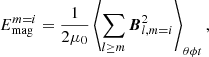
In the slowly rotating runs, sets C and D, there are changes in both radial and latitudinal differential rotation, but they are very small. Comparing the runs without the centrifugal force with those with the largest value of cf, the biggest change in  , of about 20%, is in set D. However, larger deviations are found in sets E, F, and G. They are also shown in Fig. 1 with the corresponding error bars, which were estimated by computing the average of three equally long parts of the time series and taking the largest deviation from the total as the error. In set E we see that the differential rotation of the runs that were initialized with the same cf but at a different time, namely E2 with E3 and E4 with E5, have very similar values. This shows that the averaged differential rotation does not significantly depend on the initial conditions when the centrifugal force is added. Within this set, the maximum deviation of
  is about 23% between runs E1 and E5. In contrast,
  is reduced by about 17%.
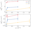 |
Fig. 1. Time-averaged differential rotation for sets E, F, and G in red, blue, and yellow, respectively. The top and bottom panels show |


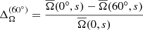
Recently, Käpylä (2023) noted that the details of the radial profile of  can introduce spurious effects into the measure of differential rotation as defined in Eq. (13). Following their approach, we defined the mean rotational profile at the equator as
![Mathematical equation: $$ \begin{aligned} \tilde{\Delta }^{(r)}_{\Omega } = \frac{\int _{r_{\rm in}}^{r_{\rm out}}r^2[\overline{\Omega }(\theta _{\rm eq},r) - 1]\mathrm{d}r}{\int _{r_{\rm in}}^{r_{\rm out}}r^2\mathrm{d}r}, \end{aligned} $$](/articles/aa/full_html/2023/10/aa46768-23/aa46768-23-eq27.gif) (15)
(15)
where rin = 0.72R and rout = 0.98R. In Fig. 2 we plot this quantity as a function of cf. The differential rotation is solar-like ( ), as already seen in the top panel of Fig. 1. This shows that, if there are transients of anti-solar differential rotation in our simulations, they are not very long and a similar scaling is seen with both definitions.
As the rotation velocity increases more, the amplitude of the latitudinal differential rotation decreases further in run F1. This is a common feature of convection in rotating spherical shells (see, e.g., Brown et al. 2008; Gastine et al. 2014; Viviani et al. 2018), which is also found in Cartesian coordinates with the star-in-a-box setup (Käpylä 2021). In runs F2 and F3,  is larger by a factor of about 2.3 and 2.6. Run F1 has bottom layers that rotate slightly faster than the surface layers, as indicated by the negative sign of
  . The addition of the centrifugal force changes this pattern back to a solar-like one, where the surface layers rotate faster, although the overall differential rotation remains weak.
We do not see major differences between runs G1 and G2, and in G3 the latitudinal (radial) differential rotation increases (decreases) by a factor of about 2 (10). Each of these runs has  and
and  . In run G4,
  is comparable to that in F2, and, similarly, the radial differential rotation is shifted back to a solar-like pattern. However, the amplitudes are all very small and close to rigid rotation. In the control simulation (G5) we took a snapshot from run G3 and switched off the centrifugal force; we obtained a solution that is nearly the same as in run G1. This hints at the possibility that the effects we are seeing are due to a systematic effect of the centrifugal force rather than a chaotic behavior due to the change in the initial conditions.
Overall, we find that changes in the differential rotation due to the centrifugal force are only noticeable in the rapidly and very rapidly rotating sets E, F, and G. We conclude that the changes in both  and
and  are due to the centrifugal force and are likely insensitive to the details of the initial conditions taken from the parent runs. In a real star, the centrifugal force would also change the geometry of the star. However, we cannot assess the extent of this change because the fixed grid in our model does not allow the geometry to change.
3.2. Magnetic energy
The magnetic energy of the first three azimuthal modes near the surface are listed in Table 2 and shown as a function of the centrifugal force amplitude in Fig. 3. It is defined as
 (16)
(16)
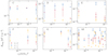 |
Fig. 3. Magnetic energy of the three lowest azimuthal modes (m) as a function of the centrifugal force amplitude. Runs with cf = 0 are given a fiducial value of cf(Ω/Ω⊙)2 = 10−4. |
Magnetic energy density from the spherical harmonic decomposition for each run in units of 105 J m−3.
where Bl, m = i are obtained from the spherical harmonic decomposition. At slow rotation, sets C and D do not show significant changes in the energy as the centrifugal force increases. At the same time, we also see that in set C the axisymmetric mode dominates the runs. This contrasts with the previous study of Viviani et al. (2018), who find that, at rotation rates larger than Ω/Ω⊙ ∼ 1.8, the m = 1 mode dominates the runs, and after Ω/Ω⊙ ∼ 20 the dominance falls back to m = 0. However, at higher grid resolutions, they find that this trend is suppressed and so the m = 1 mode dominated again. In the current simulations, we find that this trend only starts to show up in set D. In all cases, the m = 2 mode is always subdominant by a factor of roughly 10.
Similarly to the differential rotation, the effects of the centrifugal force are more noticeable in sets E, F, and G. In this rapidly rotating regime, the axisymmetric mode is always subdominant. In set E, the m = 1 mode always has the highest energy, and as the amplitude of the centrifugal force increases,  decreases and so does
  . We do not see noticeable differences between runs E2 and E3, which have the same centrifugal force but were initialized at different times. This is also the case for runs E4 and E5, meaning no hysteresis is observed and the results are independent of the history of the run. In set F, we see that the energy in the m = 0 mode decreases, and in run F2 the m = 2 mode carries most of the energy. However, when the centrifugal force is increased further, the m = 1 mode becomes dominant once again.
In run G1 there is no clearly dominating mode, and the energy in the m = 0 mode is only roughly 5% larger than in m = 1. As the centrifugal force is first added in run G2, the energy of the m = 0 mode increases by about 10%. However, similarly to run F2, run G3 has most of the magnetic energy in the m = 2 mode, which is about 66% higher than  and
and  combined. Increasing the centrifugal force further, we see that the dominant mode is m = 1, same as in the case of run F3. When the centrifugal force is switched off, the distribution of the energy goes back to levels nearer to run G1 with cf = 0.
3.3. Azimuthal dynamo waves
We began by estimating the period of the ADWs by building a periodogram and identifying the signal with the greatest power as the main cycle. We then investigated whether there are tendencies between the period of the ADW and the rotation rate in runs without the centrifugal force. This is shown in Fig. 4. From Ω = 5 Ω⊙ to Ω = 20 Ω⊙, the period of the ADWs of the m = 1 and m = 2 modes seems to increase with rotation. For more rapid rotation, the period of the m = 1 ADW decreases, whereas for the m = 2 mode this tendency appears for Ω ≥ 25 Ω⊙. For the two most rapidly rotating cases, the period of the m = 2 ADW exceeds that of the m = 1 mode.
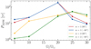 |
Fig. 4. Period of the ADWs as a function of the normalized rotation rate for runs without the centrifugal force. |
To explore the migration pattern of the ADW, we show in Fig. 5 the m = 1 mode of the radial magnetic field near the surface at a latitude of 60° for runs C1, C3, D1, D3, E1, and E5, as well as the m = 2 mode for runs F1, F2, G1, and G3. Overplotted is the advection path due to differential rotation. In Table 3 we list the periods of the ADWs at θ = 60° and the direction of the propagation.
 |
Fig. 5. ADWs for some selected runs at a latitude of θ = 60°. The top panels are the runs without the centrifugal force. The dashed line denotes the path that the ADWs would follow if they were advected by the differential rotation. For each set, we have added null data to make the time axes coincide in order to facilitate comparison. |
Properties of the ADWs.
In runs C1 and C3 we obtain a retrograde migration with no evidence of changes due to the centrifugal force. Both migration patterns appear to be constant in time with no interruptions. Similarly, the ADWs in runs D1 and D3 have a retrograde migration pattern but are characterized by a longer period. Run E1 has an interesting non-axisymmetric dynamo solution that shows periods of prograde and standing ADWs for the m = 1 mode. The migration of the ADW is changed by the centrifugal force, as evidenced by the panel for run E5. This run has a retrograde migration, similarly to sets C and D, and shows no similarity to run E1. As shown in Sect. 3.1, the change in the latitudinal differential rotation between runs E1 and E5 is about 17%. However, the ADWs propagate almost like rigid structures, so differential rotation cannot directly be used to explain their behavior. The precise origin of ADWs is unclear even in the case where the centrifugal force is absent, but quantities relevant for large-scale dynamos, such as differential rotation, kinetic helicity, and other turbulent quantities, along with their spatio-temporal profiles, likely play roles. However, the changes we observe when the centrifugal force is included suggest that subtle changes in the velocity field are enough to significantly alter the behavior of ADWs.
In run F1 the wave is standing or very slowly migrating in a retrograde direction. The migration period seems to decrease as the centrifugal force is added in the lower panel of Fig. 6, where the wave travels about 120° in azimuth. Also evident here is the increase in the magnitude of the m = 2 mode at the southern hemisphere. It also seems that this part contributes the most to the change in magnetic energy seen in Fig. 3. It is only toward the end of the simulations that the  at the northern hemisphere catches up and becomes comparable in strength to the southern hemisphere counterpart, as can be seen by comparing the panels of run F2 in Figs. 5 and 6.
In the rapidly rotating regime, the m = 2 mode of run G1 has a periodic wave with a period of about 26 years (see Table 3), with clear prograde propagation. The centrifugal force changes the propagation direction, as can be seen in the last panel of Fig. 5 (run G3), and the period of the ADW is also affected such that now it is about 70 years. In this case, the latitudinal differential rotation is doubled in run G3 as compared to run G1. Although this is the most obvious change between the simulations, it is difficult to explain the change in the ADWs with this alone, as discussed above.
In general, we find a preference for retrograde propagation, as in Viviani et al. (2018). Interestingly, however, run E1 shows a combination of standing and prograde waves and G1 is prograde. A subsequent study by Viviani & Käpylä (2021), where the prescribed heat conductivity was replaced by the Kramers opacity law, showed that there is a tendency of producing prograde-propagating ADWs. We replaced the fixed radial profile K(r) with the corresponding quantity from Kramers opacity (see Eq. (6)) and branched run E1 off to a new run, K1. The centrifugal force was added in run K2 with cf = 5 × 10⁻⁴.
Figure 7 shows the reconstructed m = 1, 2 modes for these two runs. It is clear that run E1 is different than K1, as the properties of the ADW are not reproduced when the Kramers opacity is used. In the latter case, the ADW is prograde for both m = 1 and m = 2 modes, which also have comparable energies. This is in accordance to Viviani & Käpylä (2021) in that it seems as if prograde migration is favored when the Kramers opacity is used. When the centrifugal force is added in run K2, the strength of the first non-axisymmetric mode decreases down to around 1 kG, but the direction of the propagation appears to be unaffected. Interestingly, the m = 2 mode increases from about 4 kG in run K1 to roughly 6 kG in run K2. The propagation pattern is interesting in that it seems to oscillate around a mean azimuth with an amplitude of 40° between t = 40 yr and t = 110 yr. After this, the strength of the m = 2 (m = 1) mode decreases (increases), and at around t = 150 yr the m = 2 mode reappears without a corresponding decrease in the m = 1 mode. In contrast to set E, the combination of Kramers opacity and the centrifugal force produces a dominant m = 2 mode, which was only found in the more rapidly rotating runs F2 and G3.
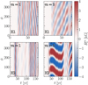 |
Fig. 7. ADWs for the runs with Kramers opacity without the centrifugal force (top) and with the centrifugal force (bottom). |
4. Summary and conclusions
In this paper we have studied the effects of the centrifugal force in semi-global dynamo simulations. It is important to assess its effects in the context of young solar analogs, which are used to study the Sun in an astrophysical context.
The amplitude of the centrifugal force is considered in our setup as a free parameter and is thus decoupled from the Coriolis term and the rotation of the star. In this way, its amplitude is artificially reduced by the control parameter cf. This allows us to avoid an unrealistically large centrifugal force (Käpylä et al. 2013). This approach was applied to a total of 21 simulations divided into five sets, each characterized by a different rotation rate and with different values of cf within each set. We find that the centrifugal force induces changes in the differential rotation and magnetic field only when rotation is rapid enough.
Both the latitudinal and radial differential rotation tend to increase with increasing centrifugal force. In the two most rapidly rotating runs without the centrifugal force, we obtained an anti-solar radial differential rotation. After including the centrifugal force, this solutions changed to solar-like differential rotation. Namely, the outer layers of the convection zone went from rotating more slowly to more rapidly relative to the deeper layers. All of our runs have a solar-like latitudinal differential rotation, where high latitudes rotate more slowly than the regions nearer to the equator. This difference increases as the centrifugal force becomes stronger (see Fig. 1).
The magnetic energy, shown in Fig. 3, also shows noticeable effects only when the rotation is rapid enough in sets E, F, and G. All runs are dominated by the m = 0 mode in set C and by the m = 1 mode in set D, and they show small changes in energy as a function of the centrifugal force amplitude. In the rapidly rotating regime, it is common to find a dominating m = 1 mode, and the energy of the m = 0 and m = 2 modes decreases as cf increases in set E. This trend is also present in sets F and G, with the difference that there are some cases where the m = 2 mode dominates.
By analyzing the ADWs near the surface of our runs, we find that the direction of the propagation changes from prograde to retrograde in some rapidly rotating runs as a function of the centrifugal force. This is most easily seen in runs E5 and G3 in Fig. 5. For run F2, we find that the direction of the propagation of the ADW is not clearly affected, but there are indications that its period might be affected (see Fig. 6).
To confirm the effects of the centrifugal force, we introduced three control runs. First, in order to test the importance of the initial conditions, we started run E3 (E5) with the same value of cf as E2 (E4) from run E1 but at a different time. There are negligible differences in the differential rotation, as can been seen in Cols. 8 and 9 of Table 1 and in the overlapping points at constant cf in Fig. 1. The magnetic energy is only slightly affected, as seen in the third panel of Fig. 3 from the data points at constant cf(Ω/Ω⊙)2. Secondly, it is important to look at the solution of a run with the centrifugal force when it is turned off again. We did this experiment with run G3, in which the propagation of the ADW was retrograde (see the last panel of Fig. 5). When the centrifugal force was turned off, the propagation changed back to prograde, as it was in the original run, G1. Overall, the control runs show that the changes described above are due to the centrifugal force and not likely the outcome of the nonlinear evolution of the equations.
A previous study by Viviani & Käpylä (2021) shows that the propagation of the ADWs can be affected by the introduction of the Kramers opacity instead of a fixed radial profile of heat conductivity. We combined the Kramers opacity with the centrifugal force in runs K1 and K2 and find that, first, the solution of the ADW is different for the runs without the centrifugal force (K1) and with the centrifugal force (K2) as compared with the corresponding runs with the spatially fixed heat conductivity (set E). Notably, run K2 showed a migration pattern that was not obtained in any of the other runs (see Fig. 7). This confirms that the Kramers opacity changes the ADW solution, but it is even more complex when the centrifugal force is included.
Despite our experiments, we were unable to identify the mechanism responsible for changing the behavior of the ADWs. The clearest change due to the centrifugal force is seen in the differential rotation, but its effect must be indirect through the dynamo mechanism because advection by a shear flow is incompatible with the practically rigidly propagating ADWs. The details of the dynamo process in 3D simulations are highly complex (e.g., Warnecke et al. 2021), and current mean-field methods are applicable only in the axisymmetric case. Observations, specifically an analysis of the surface magnetic field and its cycles as a function of rotation, could help us better understand this. Such a study was performed by Lehtinen et al. (2016), who find that the photometric rotation period and activity period of a group of stars show clear differences. They proposed that this trend could be explained by the presence of prograde ADWs. However, our simulations suggest that when a prograde wave is affected by the centrifugal force, it changes to a retrograde propagation. Such a discrepancy could be better understood by extending the observations and by performing more realistic simulations in a wider parameter regime.
Acknowledgments
We thank the anonymous referee for their comments. F.H.N. acknowledges funding from the Deutscher Akademischer Austauschdienst. F.H.N. and P.J.K. would like to thank the Isaac Newton Institute for Mathematical Sciences, Cambridge, for support and hospitality during the programme “Frontiers in dynamo theory: from the Earth to the stars” where work on this paper was undertaken. This work was supported by EPSRC grant no. EP/R014604/1. P.J.K. acknowledges the support from the Deutsche Forschungsgemeinschaft Heisenberg programme (grant no. KA 4825/4-1). P.J.K. was also partially supported by a grant from the Simons Foundation. D.R.G.S. thanks for funding via the Alexander von Humboldt Foundation, Bonn, Germany. R.B. acknowledges support by the Deutsche Forschungsgemeinschaft (DFG, German Research Foundation) under Germany’s Excellence Strategy – EXC 2121 “Quantum Universe” – 390833306. The authors gratefully acknowledge the computing time granted by the Resource Allocation Board and provided on the supercomputer Lise and Emmy at NHR@ZIB and NHR@Göttingen as part of the NHR infrastructure. The calculations for this research were conducted with computing resources under the project hhp00052.
References
- Applegate, J. H. 1992, ApJ, 385, 621 [Google Scholar]
- Brandenburg, A., Nordlund, A., & Stein, R. F. 2000, Geophysical and Astrophysical Convection (The Netherlands: Gordon and Breach Science Publishers), 85 [Google Scholar]
- Brown, B. P., Browning, M. K., Brun, A. S., Miesch, M. S., & Toomre, J. 2008, ApJ, 689, 1354 [CrossRef] [Google Scholar]
- Cang, T. Q., Petit, P., Donati, J. F., et al. 2020, A&A, 643, A39 [NASA ADS] [CrossRef] [EDP Sciences] [Google Scholar]
- Cole, E., Käpylä, P. J., Mantere, M. J., & Brandenburg, A. 2014, ApJ, 780, L22 [Google Scholar]
- Gastine, T., Yadav, R. K., Morin, J., Reiners, A., & Wicht, J. 2014, MNRAS, 438, L76 [CrossRef] [Google Scholar]
- Käpylä, P. J. 2021, A&A, 651, A66 [Google Scholar]
- Käpylä, P. J. 2023, A&A, 669, A98 [NASA ADS] [CrossRef] [EDP Sciences] [Google Scholar]
- Käpylä, P. J., Mantere, M. J., Cole, E., Warnecke, J., & Brandenburg, A. 2013, ApJ, 778, 41 [CrossRef] [Google Scholar]
- Käpylä, P. J., Käpylä, M. J., & Brandenburg, A. 2014, A&A, 570, A43 [NASA ADS] [CrossRef] [EDP Sciences] [Google Scholar]
- Käpylä, P. J., Rheinhardt, M., Brandenburg, A., et al. 2017, ApJ, 845, L23 [CrossRef] [Google Scholar]
- Käpylä, P. J., Gent, F. A., Olspert, N., Käpylä, M. J., & Brandenburg, A. 2020, Geophys. Astrophys. Fluid Dyn., 114, 8 [CrossRef] [Google Scholar]
- Krause, F., & Rädler, K.-H. 1980, Mean-field Magnetohydrodynamics and Dynamo Theory (Oxford: Pergamon Press), 271 [Google Scholar]
- Lehtinen, J., Jetsu, L., Hackman, T., Kajatkari, P., & Henry, G. W. 2016, A&A, 588, A38 [NASA ADS] [CrossRef] [EDP Sciences] [Google Scholar]
- Matt, S. P., MacGregor, K. B., Pinsonneault, M. H., & Greene, T. P. 2012, ApJ, 754, L26 [Google Scholar]
- Navarrete, F. H., Schleicher, D. R. G., Käpylä, P. J., et al. 2020, MNRAS, 491, 1043 [Google Scholar]
- Navarrete, F. H., Käpylä, P. J., Schleicher, D. R. G., Ortiz, C. A., & Banerjee, R. 2022a, A&A, 663, A90 [NASA ADS] [CrossRef] [EDP Sciences] [Google Scholar]
- Navarrete, F. H., Schleicher, D. R. G., Käpylä, P. J., Ortiz-Rodríguez, C. A., & Banerjee, R. 2022b, A&A, 667, A164 [NASA ADS] [CrossRef] [EDP Sciences] [Google Scholar]
- Reiners, A., Shulyak, D., Käpylä, P. J., et al. 2022, A&A, 662, A41 [NASA ADS] [CrossRef] [EDP Sciences] [Google Scholar]
- Skumanich, A. 1972, ApJ, 171, 565 [Google Scholar]
- Viviani, M., & Käpylä, M. J. 2021, A&A, 645, A141 [EDP Sciences] [Google Scholar]
- Viviani, M., Warnecke, J., Käpylä, M. J., et al. 2018, A&A, 616, A160 [NASA ADS] [CrossRef] [EDP Sciences] [Google Scholar]
- Völschow, M., Schleicher, D. R. G., Perdelwitz, V., & Banerjee, R. 2016, A&A, 587, A34 [NASA ADS] [CrossRef] [EDP Sciences] [Google Scholar]
- Warnecke, J., Rheinhardt, M., Viviani, M., et al. 2021, ApJ, 919, L13 [NASA ADS] [CrossRef] [Google Scholar]
- Zaire, B., Donati, J. F., & Klein, B. 2022, MNRAS, 513, 2893 [NASA ADS] [CrossRef] [Google Scholar]
All Tables
Magnetic energy density from the spherical harmonic decomposition for each run in units of 105 J m−3.
All Figures
|
Fig. 1. Time-averaged differential rotation for sets E, F, and G in red, blue, and yellow, respectively. The top and bottom panels show |
| In the text | |
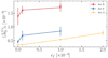 |
Fig. 2. Time-averaged radial differential rotation as defined in Eq. (15). |
| In the text | |
|
Fig. 3. Magnetic energy of the three lowest azimuthal modes (m) as a function of the centrifugal force amplitude. Runs with cf = 0 are given a fiducial value of cf(Ω/Ω⊙)2 = 10−4. |
| In the text | |
|
Fig. 4. Period of the ADWs as a function of the normalized rotation rate for runs without the centrifugal force. |
| In the text | |
|
Fig. 5. ADWs for some selected runs at a latitude of θ = 60°. The top panels are the runs without the centrifugal force. The dashed line denotes the path that the ADWs would follow if they were advected by the differential rotation. For each set, we have added null data to make the time axes coincide in order to facilitate comparison. |
| In the text | |
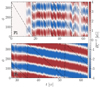 |
Fig. 6. Same as Fig. 5 but at θ = −60° for runs F1 (top) and F2 (bottom). |
| In the text | |
|
Fig. 7. ADWs for the runs with Kramers opacity without the centrifugal force (top) and with the centrifugal force (bottom). |
| In the text | |
Current usage metrics show cumulative count of Article Views (full-text article views including HTML views, PDF and ePub downloads, according to the available data) and Abstracts Views on Vision4Press platform.
Data correspond to usage on the plateform after 2015. The current usage metrics is available 48-96 hours after online publication and is updated daily on week days.
Initial download of the metrics may take a while.