| Issue |
A&A
Volume 676, August 2023
|
|
|---|---|---|
| Article Number | A16 | |
| Number of page(s) | 13 | |
| Section | Planets and planetary systems | |
| DOI | https://doi.org/10.1051/0004-6361/202346197 | |
| Published online | 27 July 2023 | |
Combination of MRO SHARAD and deep-learning-based DTM to search for subsurface features in Oxia Planum, Mars
1
Guangdong Laboratory of Artificial Intelligence and Digital Economy (SZ),
Kerun B Bld, Yutang Street, Guangming District,
Shenzhen
518107, PR China
e-mail: xiongsiting@gml.ac.cn
2
Mullard Space Science Laboratory, Department of Space and Climate Physics, University College London,
Holmbury St Mary, Dorking,
Surrey,
RH5 6NT, UK
3
Planetary Sciences and Remote Sensing Group, Department of Earth Sciences, Freie Universität Berlin,
Malteserstr. 74-100,
Berlin
12249, Germany
4
Institute for Advanced Study, Shenzhen University,
No. 3688, Nanhai Avenue, Nanshan District,
Shenzhen
518060, PR China
5
Space and Earth Interdisciplinary Center, Shenzhen University,
No. 3688, Nanhai Avenue, Nanshan District,
Shenzhen
518060, PR China
6
College of Civil and Transportation Engineering, Shenzhen University,
No. 3688, Nanhai Avenue, Nanshan District,
Shenzhen
518060, PR China
Received:
20
February
2023
Accepted:
2
June
2023
Context. Oxia Planum is a mid-latitude region on Mars that attracts a great amount of interest worldwide. An orbiting radar provides an effective way to probe the Martian subsurface and detect buried layers or geomorphological features. The Shallow radar orbital radar system on board the NASA Mars reconnaissance orbiter transmits pulsed signals towards the nadir and receives returned echoes from dielectric boundaries. However, radar clutter can be induced by a higher topography of the off-nadir region than that at the nadir, which is then manifested as subsurface reflectors in the radar image.
Aims. This study combines radar observations, terrain models, and surface images to investigate the subsurface features of the ExoMars landing site in Oxia Planum.
Methods. Possible subsurface features are observed in radargrams. Radar clutter is simulated using the terrain models, and these are then compared to radar observations to exclude clutter and identify possible subsurface return echoes. Finally, the dielectric constant is estimated with measurements in both radargrams and surface imagery.
Results. The resolution and quality of the terrain models greatly influence the clutter simulations. Higher resolution can produce finer cluttergrams, which assists in identifying possible subsurface features. One possible subsurface layering sequence is identified in one radargram.
Conclusions. A combination of radar observations, terrain models, and surface images reveals the dielectric constant of the surface deposit in Oxia Planum to be 4.9–8.8, indicating that the surface-covering material is made up of clay-bearing units in this region.
Key words: planets and satellites: terrestrial planets / planets and satellites: surfaces / planets and satellites: formation / planets and satellites: composition / planets and satellites: detection / planets and satellites: physical evolution
© The Authors 2023
 Open Access article, published by EDP Sciences, under the terms of the Creative Commons Attribution License (https://creativecommons.org/licenses/by/4.0), which permits unrestricted use, distribution, and reproduction in any medium, provided the original work is properly cited.
This article is published in open access under the Subscribe to Open model. Subscribe to A&A to support open access publication.
1 Introduction
Oxia Planum lies between 16°N to 19°N and 23°W to 28°W in a mid-latitude area on the eastern border of Chryse Planitia (Fawdon et al. 2021). It is located between two outflow channel systems, which are Mawrth Vallis to the northeast and Ares Vallis to the southwest. This region features low-relief terrain characterised by hydrous clay-bearing bedrock units and exhibits Noachian-aged terrain (Quantin-Nataf et al. 2021; Kapatza 2020). Oxia Planum comprises a considerable number of distinct geological units and shows a complex history where erosion, transport, and sedimentation are significant processes (Egea-Gonzalez et al. 2021). Within this region, Quantin-Nataf et al. analysed five characteristic surface features, which are clay-bearing units, dense mantling units, delta/fluvial fans, rounded buttes, and dark-resistant units (Quantin-Nataf et al. 2021). Thermal infrared observations from the thermal emission imaging system (THEMIS) reveal that units in this region are mainly composed of clay minerals, with some containing traces of volcanic materials (Gary-Bicas & Rogers 2021). These units are in intricate layering relationships, pointing to a complex formation history of Oxia Planum (Egea-Gonzalez et al. 2021; Gary-Bicas & Rogers 2021). Oxia Planum was selected as the landing site of the ESA ExoMars rover, which is still awaiting launch (Ivanov et al. 2020; Mastropietro et al. 2020), and so efforts have been made to analyse this region in terms of its surface characteristics and composition. This selected landing site has been shown to exhibit evidence of at least two distinct aqueous environments, both of which existed during the Noachian (Quantin-Nataf et al. 2021). To support geologic interpretation, many datasets have been produced and released to the public, including multi-source surface imagery and topographic data (Quantin-Nataf et al. 2021; Tao et al. 2021b).
Shallow radar (SHARAD) is an orbital radar system on board the NASA Mars reconnaissance orbiter (MRO), and its acquired dataset has been widely used to investigate the subsurface features of Mars. This instrument operates at a frequency of 10 MHz and transmits pulsed signals towards the nadir while it orbits the planet (Seu et al. 2004). Generally, most of the incident wave is reflected at the surface of Mars as it encounters the interface between free space and the subsurface. However, a relatively small portion of the incident waves can be transmitted to the subsurface region. When the transmitted waves encounter another dielectric boundary, they are reflected and received by the instrument at a delayed time interval. The radar receiver measures a stronger reflection than the background noise when the radar signal is reflected at a proper dielectric boundary. The depth imaged by this instrument depends not only on the transmitted power but also on the subsurface material properties. SHARAD data have been used to study the composition of the Martian polar regions, and layered deposits have been revealed on both the south and the north poles (Picardi et al. 2005; Plaut et al. 2007; Smith et al. 2016; Xiong & Muller 2019; Brothers et al. 2015). Subsurface features have also been revealed in the equatorial regions on Mars, including the Medusae Fossae Formation (MFF; Carter et al. 2009), Utopia Planitia (Stuurman et al. 2016), Elysium Planitia (Xiong et al. 2021), and debris-covered glaciers (White 2017).
The signals received from the nadir footprints along the flight path form an image called a radargram. Subsurface features are recognisable in the resulting radargram either by visual inspection or by automated detection (Xiong & Muller 2019). The nadir-looking implies a left–right range ambiguity and a subsurface and superficial range ambiguity (Spagnuolo et al. 2011). The received echo is a combination of nadir surface echo, nadir subsurface echo, off-nadir surface echoes, and off-nadir subsurface echoes. The surface echoes can be simulated using digital terrain models (DTMs). The simulated image has the same dimensions as the radargram and is termed a cluttergram (Nouvel et al. 2004; Spagnuolo et al. 2011; Choudhary et al. 2016). Comparisons of radargrams and cluttergrams assist in excluding surface echoes and identifying the possible subsurface features. However, further studies of the influence of the quality and resolution of DTMs on the simulated cluttergram and its aided subsurface feature identification are required.
The aim of this study is to provide new insights into the geological history of the Oxia Planum. To this end, we map subsurface features in this region by combining SHARAD radar-grams and simulated cluttergrams. The study area and related datasets are introduced in Sect. 2. To facilitate this work and provide insight into future work, in Sect. 3 we establish a workflow that integrates datasets, software, and tools that are helpful in the subsurface mapping of Mars, and in Sect. 4 we present our experimental results. Finally, certain shortcomings of the workflow, data processing, and analysis are discussed in Sect. 5, and the conclusions of our study are outlined in Sect. 6.
2 Study area and datasets
The coverage of the area of Oxia Planum by the different instruments is illustrated in Fig. 1. Surrounding the proposed landing site, there are three main geological units, namely the early (eNh), middle (mNh), and late Noachian highlands (1Nh). In addition to SHADAR, which is collecting profiling images of the Martian subsurface, many orbital sensors and imaging systems are covering this region, such as the high-resolution stereo camera (HRSC; Scholten et al. 2005) on board the Mars Express (MEX) mission, and the context camera (CTX; Malin et al. 2007) and high-resolution imaging science experiment (HiRISE; Neukum & Jaumann 2004) on board the Mars reconnaissance orbiter (MRO) mission. Figure 1 shows the areas of Oxia Planum for which data have been collected for this study. The base map is the hill-shaded Mars orbiter laser altimeter (MOLA) DTM overlaid by a colourised HRSC DTM. The black box is the bounding box of the CTX DTM, and the serrated edge denotes the boundary between valid data and no data areas. In the following paragraphs, we introduce the SHARAD data, the primary data used to search for the subsurface features, and then the surface DTMs and images, which assist in interpreting the subsurface findings.
2.1 SHARAD data
SHARAD on board MRO is a nadir-looking orbiting radar. It transmits chirps lasting 85 µs at a central frequency of 20 MHz with a bandwidth of 10 MHz and power of 10 W. Due to its low frequency, it penetrates the Martian subsurface to a depth of up to several kilometres. The radar instrument collects a profile of radar return echoes along its flight path. The returned echoes form an image with a fast time axis representing the nadir direction and a slow time axis representing the flight direction.
The acquired raw data are processed by US and Italian mission collaborators separately with different image-focusing algorithms. The data are publicly available at the Planetary Data System (PDS) of the Geosciences Node1. According to the data specification (Campbell 2014), the column number (slow time axis) is determined with the footprints stored in the orbit file. The distance spacing between each column is ~463 m as the released data have been resampled with the same spacing interval as the MOLA gridded DTM. The row number of the radargram (fast time axis) is 3600 for all products. The middle row of the radargram (1800th row) has been coregistered to the free-space, round-trip time delay of the MOLA-defined Mars areoid.
In this study, we searched the SHARAD product using the bounding box of the CTX DTM and the global coverage of SHARAD data2. As the data are almost spontaneously updated at the PDS (updated to May 25, 2022), we also searched the data obtained by the Mars Orbiter Data Explorer at the PDS that cover the same area. Finally, 112 SHARAD radargrams are found to cover the study area (the latest orbit number is 6579 updated on December 20, 2022).
The standard SHARAD products are released as long tracks, which may significantly exceed our study area. To focus on this specific area, we cropped the radargram using the extent of the CTX DTM. After processing, 87 of these radargrams are identified as being located within the bounding box of the CTX DTM. The grey lines in Fig. 1 show the footprints of all SHARAD products crossing this bounding box. Three of the collected products (PID: 02622401, 04743502, and 06289603) are coloured as cyan lines on the radargrams and the corresponding cluttergrams are demonstrated in Sect. 4.1 as examples. The product shown as an orange line in Fig. 1 (PID: 05594002) contains one possible subsurface layer sequence, which is analysed in detail in Sects. 4.2 and 4.3.
2.2 Martian DTMs
The MOLA gridded DTM has been intensively used in the clutter simulation due to its global coverage (Smith et al. 2001; Christoffersen et al. 2022). It has a resolution of 128 points per degree, with each degree representing ~463 m, similar to the SHARAD resampling distance.
In addition to laser altimetry, stereo photogrammetry is another valuable technique for producing topographic data. Stereo photogrammetry requires two images, one from each of two slightly different viewing angles, to estimate the depth from the imaging point, analogously to the human visual system. Stereo photogrammetry can be applied to HSRC, CTX, and HiRISE images to produce DTMs. The resolutions of the derived DTMs are 50 m, 18 m, and 50 cm, respectively.
In addition to stereo photogrammetry (Tao et al. 2021a), shape-from-shading (Douté & Jiang 2019) and deep-learning-based methods (Chen et al. 2021; Tao et al. 2021b,c,d) have been developed, and can produce high-resolution Martian DTM products. In particular, a deep learning network called multi-scale generative adversarial U-Net with dense convolutional and up-projection blocks (MADNet; Tao et al. 2021b,c) has been applied to produce higher-resolution and better-quality DTMs using single images from HRSC, CTX, and HiRISE over the Oxia Planum landing site. The MADNet network uses a three-scale U-Nets-based architecture to encode the input as features at coarse, intermediate, and fine scales, which are then fed into five stacks of up-projection blocks and convolutional layers with concatenations of the corresponding outputs of each pooling layer to decode the features into the output height map. The produced datasets of the Oxia Planum have been released to the public at the ESA Guest Storage Facility (GSF) repository3. The resolutions of the MADNet DTMs are higher than those derived by stereo photogrammetry, which are 25 m, 12 m, and 25 cm for HRSC, CTX, and HiRISE DTMs, respectively.
Apart from SHARAD data and Martian DTMs, surface imagery is used as it reflects the surface spectral properties. Different geological units can be recognised by their different appearance in the surface imagery. High-resolution panchromatic imagery is necessary to identify any exposed layers on the surface that may be associated with the subsurface features in this area. HiRISE imagery provides the highest resolution image of Mars from orbit, which reaches 25 m pixel−1. Unfortunately, there is no HiRISE coverage of our study area. Therefore, we use CTX images to analyse exposed surface layers.
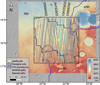 |
Fig. 1 Area of Oxia Planum surrounding the proposed landing site of the ESA ExoMars rover, with the coverage by SHARAD and CTX highlighted. See inset for details of the areas covered by these instruments. The yellow dot indicates the location of the ExoMars landing site. The three main geological units of the Noachian highlands are shown: eNh, mNh, and 1Nh. The grey lines within the black box are the paths of the SHARAD radargrams. Three paths are annotated as cyan lines and example radargrams are shown in Fig. 5. |
3 Methods
Radar observation and terrain models are two datasets that are necessary to identify possible subsurface features of the Martian upper crust. As part of this study, we developed a data-processing flow to combine surface terrain models, radar observations, surface imagery, and other possible data sources, such as thermal and multi-spectral remote-sensing observations, to map and analyse subsurface features, as shown in Fig. 2. SHARAD data processing, clutter simulation, and dielectric constant estimation are three key components.
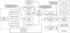 |
Fig. 2 Overall workflow, datasets, and tools used in the subsurface mapping of Mars. |
3.1 SHARAD data processing
In a previous study, we developed an automated data processing package (SHARAD3d) for SHARAD data. This package carried our SHARAD data processing, including reading and writing image and geometry files, automatic subsurface feature detection, and clutter simulation, and was successfully used in the subsurface mapping of Promethei Lingula (Xiong & Muller 2019) and Elysium Planitia (Xiong et al. 2021), both on Mars. As revealed in previous publications, subsurface layers are abundant in the Martian polar regions but are less often observed in equatorial regions.
Generally, visual inspection and validation of the observed subsurface reflections are necessary, which is especially important in equatorial and mid-latitude regions where surface composition usually results in low subsurface echoes, which are difficult to differentiate from noise. This situation holds for Oxia Planum, where no subsurface features can be automatically identified with confidence. Therefore, visual comparison between radargram and cluttergram is necessary in order to identify the subsurface features but is costly in terms of labour. To improve the efficiency of visual inspection between radargrams and simulated cluttergrams, we present a new QGIS-plugin called SHARADViewer. This consists of four viewing windows showing the radargram, the corresponding cluttergram, the cropped DTM used for the simulation, and the topographic profile, respectively.
3.2 Clutter simulation
In order to simulate clutter, we collected both HRSC and CTX MADNet DTMs and compared their clutter simulation results against the results based on the MOLA DTM. The identification of possible subsurface features is based on comparisons between radargrams and corresponding simulated cluttergrams.
For each nadir footprint, radar imaging geometry with regard to the surface topography is illustrated in Fig. 3, where A is the position of the MRO with SHARAD on board, and O is the mass centre. S and P denote the nadir surface point and one off-nadir surface point, respectively. The pseudo-code for producing the cluttergram is listed in Table 1, and the theory is described as following.
Let us say that the P′ is the clutter caused by P. In this case, we have AP = AP′. The simulation of clutter consists in determining the power of off-nadir reflectance projected in the nadir direction, which can be denoted as Pr(i, j), where (i, j) are row and column numbers in the cluttergram. Therefore, the row number i of the P′ in the radargram can be calculated using the time delay corresponding to BP′ in Fig. 3:
 (1)
(1)
where ΔT is the double-way time delay of one pixel in the radar-gram, which is 0.0375 µs according to the data specification. Furthermore,  and tab can be calculated using AP′ and AB according to the geometry BP′ = AP′ – AB. Combining with AP′ = AP, there is BP′ = AP – AB.
AP can be derived using the triangle APC as
 (2)
(2)
where PC can be calculated using the map coordinate, (xp, yp), of point P. For calculating AC, we can have an approximation of PO ≈ CO because PO ≫ AP. Here, AC corresponds to the difference between the distances of A and P to the mass centre, O, which is ha – hp. Therefore, we have
 (3)
(3)
where Δxp, Δyp, and Δhp are xp – xc, yp – yc, and ha – hp, respectively. The (xc, yc) are the coordinates of the point S. Then, the time delays, tap′ in Eq. (1) can be calculated as
 (4)
(4)
where C is the speed of light.
To calculate tab, we need to know AB which can be expressed as AB = AO – BO, in which AO and BO correspond to the heights of MRO, ha, and Martian aeroid to the mass centre, hb. These two parameters vary along the flight path of SHARAD and are recorded in the geometry file. Then, the time delay, tab, can be calculated using
 (5)
(5)
Finally, the relationship between row number in the clutter-gram and DTM sampling point, (xp, yp, hp) can be expressed by substituting Eqs. (5) and (4) into Eq. (1), as follows:
 (6)
(6)
Although SHARAD data have been corrected with MOLA DTM, the first echo return may not be confirmed to the nadir surface point. Therefore, we project the nadir surface footprints back onto the cluttergram to compare this projection with the first echo return. The row number of the surface point, S, can also be calculated by substituting (xs, ys, hs) into Eq. (6).
The power received by the radar instrument from the Martian surface can be modelled using the radar equation (Brown 1949):
 (7)
(7)
where Pt is the transmitted power, G0 the antenna gain, λ the wavelength of the radar, R the range from the instrument to the surface element, and σ the backscattering coefficient of the surface element Λ, which relates to the incident elevation angle θ and the azimuth angle ϕ.
DTMs are in a gridded format, in which each pixel can be regarded as a facet. Then, the received power of (x, y) in the cluttergram can be approximated by the sum of the backscattering of all facets (x, y) ∊ Ω projected to the same pixel in the radargram, as Ω → (i, j). This is expressed as
 (8)
(8)
where K is a constant and R can be calculated using (x, y, h) in the DTM. The σ is related to (θ, ϕ), which can also be derived from the DTM. Therefore, the key question is how to model the backscattering coefficient with surface property.
Hagfors model (Hagfors 1964) has been extensively used in the planetary science community for quasi-specular scattering which can consistently fit many near-nadir backscatter observations (Shepard & Campbell 1999), which is the case for SHARAD observations. According to Hagfors model, as in Eq. (8) of Biccari et al. (2001), the σ can be approximated using
 (9)
(9)
where Γ is the Fresnel reflectivity at the incident elevation angle, which is given with the real dielectric constant of the crust evaluated at the surface:
 (10)
(10)
and the parameter mf is derived from the value of σ computed for θ = 0, under the Kirchhoff approximation (surface gently undulating), as
 (11)
(11)
where H is the Hurst exponent, which has a high probability of lying in the range of 0.6−1. In the study of time series, the Hurst exponent (Hurst 1951) is used to analyse stochastic properties, and is also commonly used in surface science for measuring surface roughness (Mandelbrot 1977). The rms slope sλ is evaluated between points separated by a distance equal to the transmitted wavelength, as
 (12)
(12)
where Δx0 is a step size, and Δx = λ.
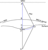 |
Fig. 3 Imaging geometry of SHARAD onboard MRO and the surface topography. |
Pseudo-code for producing the cluttergram.
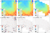 |
Fig. 4 Comparison of different Martian DTMs: (a) The MOLA DTM, (b) the MADNet HRSC DTM and the MADNet CTX DTM, with (c) to (f) showing the elevation difference maps between the two. |
3.3 Dielectric constant estimation
Once the subsurface layers are identified after the comparison, the surface terrain model and panchromatic images are investigated for related associated exposed layering sequences. After finding the correspondence between subsurface layers and exposed layers, the dielectric constant, ϵ, of the surface deposited material is estimated as
 (13)
(13)
where n = Iss – Is is the row number difference between the subsurface and surface layers observed in the radargram (measured as a unit in pixels), and d denotes the depth of the subsurface layer to the Martian surface. This depth needs to be measured on site, which, in this case, is not applicable. In this study, this depth is measured as the elevation difference between the surface and the exposed subsurface layer, which can be identified in the surface imagery and measured in the surface terrain model.
4 Results
4.1 Clutter simulation based on different DTMs
Before comparing the clutter simulation results, we first evaluate the MADNet DTMs taking MOLA DTM as a reference. The comparison between the HRSC MADNet and CTX MADNet DTMs and the MOLA DTM is demonstrated in Fig. 4. Overall, the HRSC MADNet and CTX MADNet DTMs are well co-aligned with the MOLA DTM, except that more detailed variations can be seen in the HRSC MADNet DTM compared to the CTX MADNet DTM.
For all radargrams, we simulate the cluttergram using MOLA, HRSC, and CTX DTMs. The radargram and clutter-grams are scaled to 0–255 with grey and blue colour scales, respectively. In Fig. 5, three examples are shown in order to demonstrate the different clutter simulations based on different DTMs. The figures in the first row are original radargrams, with the orange dots denoting the projection of the nadir elevations using HRSC DTM. We can see an offset between the orange dots and the surface reflectors in the radargram of 04743502. This offset may result from the correction of the radargram, as the SHARAD radargram has been corrected with the MOLA DTM as described in the data specification (Campbell 2014).
From Fig. 5, we can see that, overall, the MOLA simulations resemble the filtered results of the other two simulations, and the HRSC simulations appear noisier than the CTX simulations. In Fig. 5, reflections of RL1–6 in the radargrams correspond to the clutter, CL1–6, in the cluttergrams. Comparisons between RL2, RL3, RL5, and RL6 and CL2, CL3, CL5, and CL6, respectively, demonstrate that the simulated clutter is less obvious in the MOLA simulation than in the HRSC and CTX simulations. It should also be noted that the MOLA simulation shows no clutter at the location of RL1 and RL4, while the HRSC simulation shows a faint feature and the CTX simulation shows obvious clutter corresponding to RL1 and RL4.
These comparisons show that the HRSC MADNet and CTX MADNet DTMs are superior to the MOLA DTM in their ability to simulate finer clutter. CTX MADNet DTM performs slightly better as it is less noisy than the HRSC MADNet DTM. However, the CTX DTM has a smaller coverage than the HRSC DTM, leading to areas with no data in the last row of panels in Fig. 5. Although we have less confidence in their ability to identify clutter, we used the HRSC simulations in the areas where CTX simulations are not available.
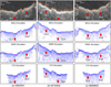 |
Fig. 5 Comparison between clutter simulations based on MOLA, HRSC MADNet and CTX MADNet DTMs. Resultant simulations along the SHARAD observations: (a) 02622401; (b) 04743502 and (c) 06829603. RL1–6 are radar reflectors and CL1–6 point to the location of corresponding clutters. The orange dots in the first-row subfigures are projections of nadir surface to the radargram coordinate. |
4.2 Subsurface feature extraction
In this study area, SHARAD receives return echoes with diminished power, resulting in few prominent reflectors. After visually inspecting all the SHARAD radargrams and comparing them with their corresponding cluttergrams, only one radargram (PID: 05594002) attracts our interest, which is because it appears to contain three sets of layer-like features. In Fig. 6a, the original radargram is demonstrated along with the clutter simulations based on MOLA, HRSC, and CTX DTMs as shown in (b–d), respectively. The interesting region is highlighted with the red box in (a), in which the red, yellow, and green arrows point to three faint layers just south of the Malino Crater, which is a degraded impact crater of 15 km in diameter. The floor of the crater is covered by low-relief, dark-toned material that overlaps light-toned terrain at breaches in the crater rims to the north and east (Fawdon et al. 2021). The layer pointed out by the red arrow is dubious as the cluttergrams in Figs. 6b,c show clutter near the observed layers. Left of the red arrow, the yellow and green arrows point to another region with two possible layers. This region is about 18 km away from the south rim of the crater. The upper layer set (with yellow arrow) is close to the lower boundary of the simulated clutter, while there appear to be no clutter in the region of the lower part (green arrow).
Figure 7a shows a close-up view of the original radargram within the red box area in Fig. 6, along with the radargram after application of the Log-Gabor filter (Gabor 1946), the MOLA cluttergram, and the HRSC cluttergram, which are shown in Figs. 7c–d, respectively. The black dots in Fig. 7b show the features extracted using the continuous wavelet transform (CWT). Among the extracted points, three sets of them seem to form three layers, which are highlighted in the red, yellow, and green ovals, respectively. Each of the three ovals corresponds to the arrow in the same colour shown in Fig. 6a. Comparing Figs. 7a,b against c and d, the layer annotated by the green oval is the most likely to be an unusual layer, while the other two are much closer to the simulated clutter. The solid red line in Fig. 7 spans Cols. 53–68, while the dotted red line spans Cols. 69–84.
To examine the echo strength of these areas, radar echoes and simulated clutter echoes are extracted along these columns and plotted in Fig. 8. The black and grey arrows in Fig. 8 show the possible locations of subsurface echoes. It can be seen from Fig. 8a that along Cols. 54–56, 62–64, and 66, the echo strengths of the arrow point location are higher than the strength of the surface echoes, while for the others (grey arrows), though higher than the background noise, the echo strength accounts for less than one-third of the surface echo strength. The row numbers of surface and subsurface echoes along Cols. 53–82 are measured and listed in Table 2. Due to more considerable echo strength and subsurface echo continuity, measurements along Cols. 53–68 are regarded as more reliable than the others. The average n calculated using measurements along these columns is 34.0, while this is 31.0 when using all measurements in Table 2.
From Cols. 62–67, we can see stronger echoes around row 2320. These echoes are not regarded as being related to subsurface layers because of the appearance of peak echoes in the HRSC cluttergram near row 2320. It should be noted that these stronger peak echoes correspond to the area pointed out by the yellow arrow in Fig. 7b, which is likely to be caused by clutter. In addition, some high peak echoes appear just before row 2360, such as Cols. 56 and 57. These high peak echoes may be due to noise in the HRSC DTM. Alternatively, this may result from the fact that we do not consider the side-lobe effect of the radar-transmitted signal. The radar side-lobe pointing to the side areas is weaker than that along the nadir direction, which means surface clutter from long range should be much weaker than that from close range. This effect has not been considered in the clutter simulation, which may lead to stronger clutter in the deeper part.
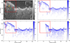 |
Fig. 6 Three sets of unusual subsurface layers (highlighted with the red, yellow, and green arrows) suspected to be found in the (a) SHARAD radargrams (PID: 05594002), and comparisons with the (b) MOLA cluttergram, (c) HRSC cluttergram, and (d) CTX cluttergram. A close-up view of this area is shown in Fig. 7 with corresponding clutter simulations based on MOLA and HRSC DTMs. |
 |
Fig. 7 Close-up view of the area of interest from (a) the original radargram with normalised echo strength, (b) the radargram with the log-Gabor filter applied, (c) the MOLA cluttergram, and (d) the HRSC cluttergram. The red, yellow, and green ovals show each of the three sets of unusual subsurface layers. In the green oval, the red solid line spans from Cols. 53 to 68, and the red dotted line ranges from Cols. 69 to 82. |
 |
Fig. 8 Radar reflections and simulations along (a) Cols. 53–68 and (b) Cols. 69–84 of the selected radargram (PID: 05594002), with the black and grey arrows pointing to the echoes caused by the possible subsurface layer, which corresponds to the area highlighted with the green arrow in Fig. 6 and the green oval in Fig. 7. |
Row numbers of surface (Is) and subsurface (Iss) reflections extracted from the interesting radargram acquired south of the Malino Crater (PID: 05594002).
4.3 Dielectric constant estimation
With the revealed possible layer, in this section, we attempted to find its manifestation of surface indicators from the surface imagery. This analysis is carried out in the Quantum GIS (QGIS) system as demonstrated in Fig. 9. In Fig. 9a, the hill-shaded HRSC DTM is overlaid by the CTX mosaic image. The region of interest is located at the southern rim of the Malino Crater, which is just at the boundary of the northern 1Nh and southern mNh. Northeast of the crater is one region of dark resistant units surrounded by the clay-bearing units, which have a thickness of more than 50 m. These clay-bearing units can be further divided into two types according to their different possible compositions, which are iron-rich alteration minerals mixed with olivine, or Fe/Mg phyllosilicate and hematite mixed with carbonates (Krzesińska et al. 2021; Mandon et al. 2021).
Figure 9a shows the close-up view of the area surrounding the Malino Crater. The base map of the CTX mosaic image is overlaid by the hill-shaded HRSC DTM and contour lines of the CTX DTM. The footprint (AA’) of the interesting SHARAD data (PID: 05594002) is plotted as the orange line, along which the elevation profile is demonstrated in Fig. 9b. To delineate the subsurface layer in the elevation profile, we need to assume a dielectric constant for the covering material. The two purple lines in Fig. 9b denote two cases of the subsurface layer with the dielectric constant set to 1 and 10, respectively. A linear fit is applied to the distance and elevation, and the two results are plotted as the dotted magenta lines. Moreover, we calculate the average elevation of the fitted line with regard to varying dielectric constant between 1 and 10, as shown in the subset figure in (b), in which the elevation ranges from −3026 to −2907 m.
In the next step, we attempt to find the exposed layer representing the apparent division of different deposits, and match the subsurface layer. First, we focus on the southern rim of the Malino Crater in Fig. 9c. Two subtle divisions on the exposed rim slope can be observed, annotated by the dashed red lines. From the contours overlying the image, it can be seen that the elevation of these faint layers is around −2940 m. If this layer is regarded as the correspondence of the subsurface layer, then the dielectric constant can be estimated to be 3.9.
Meanwhile, it is worth noting that there is another smaller crater east of the Malino Crater. The southern rim of this crater seems better preserved than that of the Malino Crater, as shown in Fig. 9d. Notably, one terraced layer can be clearly seen in the elevation range between −2930 and −2910 m. These elevations correspond to dielectric constants from 4.9 to 8.8 if the terrace layer is regarded as being a match to the subsurface layer. The subsurface layer is more likely to match the terrace layer than the faint layer in c, given that the latter appears to be more severely eroded than the former. This match is also more likely as the dielectric constant of olivine and phyllosilicate is between 6 and 10 (Biccari et al. 2001). With the estimated dielectric constant ranging between 4.9 and 8.8, the thickness of the upper covering material can be calculated to be ranging from 58 to 78 m according to the observed subsurface echoes. Regarding that this region shows an abundance of clay-bearing units of a thickness of more than 50 m, we suspect that the observed layers in the SHARAD radargram could form a boundary within the clay-bearing units, which may be composed of clay and olivine.
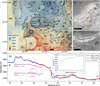 |
Fig. 9 Surface imagery showing exposed layers at the crater rim. (a) Base map of the CTX mosaic image overlaid by the hill-shaded HRSC DTM and contour lines of the CTX DTM. The orange line shows the footprint of the radargram of 05594002 in this region, (b) Elevation profiles along AA’ of the radargram. The possible subsurface layer is delineated as the purple solid lines with the magenta dotted line showing the linear fit of them, respectively, (c) Close-up view of the southern rim of the Malino Crater and (d) a close-up view of the southern rim of one smaller crater with contour lines in black and dashed lines with red showing the exposed layers. |
5 Discussion
We realised clutter simulations using different DTMs and compared them over the Oxia Planum landing site. Simulation results demonstrate that the higher the resolution of the DTM, the finer the detail of the clutter simulation. Previous interpretations of SHARAD data were hindered by limited coverage of high-resolution DTMs. This study shows that confidence in excluding clutter and identifying subsurface features from SHARAD data can be largely improved with our single-image-based DTM estimation method (Tao et al. 2021b,c). It is especially important to compare different simulations as this kind of study has no ground truth validation. However, detecting and identifying subsurface layers in SHARAD radargrams by excluding clutter in the cluttergram is hard to fully automate due to the complex terrain and faint layers of the region surrounding Oxia Planum. Manual intervention is still needed to guarantee reliable detection of subsurface layers, and the SHARADViewer QGIS plugin is developed to alleviate the manual work in this study. More highly automated methods are needed in order to reduce and eventually eliminate this manual work; these could be based on deep learning or artificial intelligence.
One problem associated with the estimation of the dielectric constant is the difficulty in establishing the correspondence between the observed radar reflectors in the SHARAD data and the exposed layers in surface imagery. In this study, the possible layer found in the SHARAD radargram is matched with the exposed layer on the crater rim. We believe that the layer preserved after surface erosion processes is more likely to be a subsurface layer extending further south. The dielectric constant estimation is based on the inference that the dielectric and radiation properties of two distinctive layer sequences can be in large contrast, leading to layers observed in both surface imagery and radar data. However, the link between these different types of layering phenomena is weak for several reasons. On the one hand, the long distance of the possible layer to the crater rim and the limited resolution of surface imagery make it difficult to associate this layer with a corresponding exposed layer. On the other hand, the radar reflectors are the dielectric boundary, while the exposed layers reflect the boundary due to differences in surface reflectance. It is hard to reach a definitive conclusion as to whether or not these two types of boundary are caused by the exact same subsurface layer. In the future, differences in the physical mechanism causing layering in these two data types should be further studied.
Data provided by the Observatoire pour la Mineralogie, l’Eau, les Glaces et l’Activité (OMEGA) and Compact Reconnaissance Imaging Spectrometer for Mars (CRISM) reveal that the minerals in this region are typical of Fe/Mg clays and the dominant spectra match that of a vermiculite-smectite type of clay (Carter et al. 2015). If this type of clay accounts for a large percentage of the surface deposited material, the radar signals may be largely absorbed, which would mean that no layers would observed in a SHARAD radargram. Unlike the Elysium Planitia, the rough surface and dense craters in this region can also reduce the transmitted energy of the radar signal because of the stronger diffuse reflections. This phenomenon may explain why so few subsurface features are observed, and why this layer-like feature is not observed in more than one SHARAD profile. Comparative studies should be carried out to investigate the influence of surface roughness, surface composition, and terrain relief on the applicability of SHARAD data in searches for subsurface features.
6 Conclusions
With this study, we provide a workflow combining subsurface radargrams and surface imagery to investigate the subsurface features on Mars based on previous studies. This workflow can be applied in future work to search for subsurface features in other regions on Mars. Deep-learning-based DTMs are used in this workflow for clutter simulation. Our analyses demonstrate the good performance of MADNet DTMs in simulating clutter and in helping identify subsurface features in SHARAD radar-grams. Within the study area, three possible subsurface layering sequences are observed in one radargram acquired south of the Malino Crater. Two of these observed layering sequences are less likely to be subsurface features. In contrast, one lower layering sequence is believed to be a possible subsurface layer after comparing radargrams with simulated cluttergrams. In addition, we tried to match this possible subsurface layer to the exposed layers on the slope of the crater rims and estimate the dielectric constant of surface deposits, which we find to be in the range of 4.9–8.8. Based on comparisons with published studies that analyse the geological units and formation of the Oxia Planum, this estimation indicates that the surface deposits are likely clay-bearing units.
The possible subsurface layering sequence is observed in only one SHARAD radargram. We are still facing the challenge that the existing SHARAD system has a lower detection limit that appears vary between repeat observations. Further observations are required in order to confirm the existence of the possible subsurface layer sequence reported here. As discussed in the previous section, from a technical perspective, this calls for more advanced methods to mitigate or eliminate the manual work involved in inspecting the radargrams and their comparison with cluttergrams, and also for the inclusion of other remote sensing datasets, such as thermal and multi-spectral datasets, including THEMIS and CRISM. From a scientific perspective, the performance of subsurface detection based on orbital radar data requires further evaluation and analysis by comparative studies across different geographical locations and geologic units.
Acknowledgements
This work is supported by the Shenzhen Science and Technology Innovation Commission (Grant No. JCYJ20190808120005713), and Guangdong Basic and Applied Basic Research Foundation (Grant No. 2022A1515110861). Part of this work was supported by funding from the National Natural Science Foundation of China (Grant No. 42004099 and 42241139), the UKSA Aurora programme (2018–2021) (Grant No. ST/S001891/1), and the STFC MSSL Consolidated Grant of United Kingdom (Grant No. ST/K000977/1).
References
- Biccari, D., Picardi, G., Seu, R., & Melacci, P. 2001, Int. Geosci. Remote Sens. Symp., 6, 2560 [Google Scholar]
- Brothers, T., Holt, J., & Spiga, A. 2015, J. Geophys. Res. Planets, 120, 1357 [NASA ADS] [CrossRef] [Google Scholar]
- Brown, R. H. 1949, Nature, 164, 810 [NASA ADS] [CrossRef] [Google Scholar]
- Campbell, B. 2014, U.S. Shallow Radar (SHARAD) data product description for the planetary data system, https://pds-geosciences.wustl.edu/mro/mro-m-sharad-5-radargram-v2/mrosh_2101/document/rgram_processing.pdf [Google Scholar]
- Carter, L. M., Campbell, B. A., Watters, T. R., et al. 2009, Icarus, 199, 295 [NASA ADS] [CrossRef] [Google Scholar]
- Carter, J., Loizeau, D., Quantin, C., et al. 2015, in EGU General Assembly Conference Abstracts, 5810 [Google Scholar]
- Chen, Z., Wu, B., & Liu, W. C. 2021, Remote Sens., 13, 839 [NASA ADS] [CrossRef] [Google Scholar]
- Choudhary, P., Holt, J. W., & Kempf, S. D. 2016, IEEE Geosci. Remote Sens. Lett., 13, 1285 [CrossRef] [Google Scholar]
- Christoffersen, M. S., Holt, J. W., Kempf, S. D., & O’Connell, J. D. 2022, SHARAD Surface Clutter Simulations PDS Archive User’s Guide, https://pds-geosciences.wustl.edu/mro/urn-nasa-pds-mro_sharad_simulations/document/userguide.pdf [Google Scholar]
- Douté, S., & Jiang, C. 2019, IEEE Trans. Geosci. Remote Sens., 58, 447 [Google Scholar]
- Egea-Gonzalez, I., Jiménez-Díaz, A., Parro, L. M., et al. 2021, Icarus, 353, 113379 [NASA ADS] [CrossRef] [Google Scholar]
- Fawdon, P., Grindrod, P., Orgel, C., et al. 2021, J. Maps, 17, 621 [CrossRef] [Google Scholar]
- Gabor, D. 1946, J. Institution Elec. Eng. Part III Rad. Commun. Eng., 93, 429 [Google Scholar]
- Gary-Bicas, C., & Rogers, A. 2021, J. Geophys. Res. Planets, 126, e2020JE006678 [NASA ADS] [CrossRef] [Google Scholar]
- Hagfors, T. 1964, J. Geophys. Res., 69, 3779 [NASA ADS] [CrossRef] [Google Scholar]
- Hurst, H. E. 1951, Trans. Am. Soc. Civil Eng., 116, 770 [CrossRef] [Google Scholar]
- Ivanov, M., Slyuta, E., Grishakina, E., & Dmitrovskii, A. 2020, Sol. Syst. Res., 54, 1 [CrossRef] [Google Scholar]
- Kapatza, A. 2020, Master’s thesis, University College London, UK [Google Scholar]
- Krzesińska, A. M., Bultel, B., Loizeau, D., et al. 2021, Astrobiology, 21, 997 [CrossRef] [Google Scholar]
- Malin, M. C., Bell, J. F. III, Cantor, B. A., et al. 2007, J. Geophys. Res. Planets, 112, E5 [CrossRef] [Google Scholar]
- Mandelbrot, B. 1977, Fractals (San Francisco: Freeman San Francisco) [Google Scholar]
- Mandon, L., Parkes Bowen, A., Quantin-Nataf, C., et al. 2021, Astrobiology, 21, 464 [NASA ADS] [CrossRef] [Google Scholar]
- Mastropietro, M., Pajola, M., Cremonese, G., Munaretto, G., & Lucchetti, A. 2020, Sol. Syst. Res., 54, 504 [NASA ADS] [CrossRef] [Google Scholar]
- Neukum, G., & Jaumann, R. 2004, EAS 1240, 17 [NASA ADS] [Google Scholar]
- Nouvel, J.-F., Herique, A., Kofman, W., & Safaeinili, A. 2004, Rad. Sci., 39, 1 [Google Scholar]
- Picardi, G., Plaut, J. J., Biccari, D., et al. 2005, Science, 310, 1925 [NASA ADS] [CrossRef] [Google Scholar]
- Plaut, J. J., Picardi, G., Safaeinili, A., et al. 2007, Science, 316, 92 [NASA ADS] [CrossRef] [Google Scholar]
- Quantin-Nataf, C., Carter, J., Mandon, L., et al. 2021, Astrobiology, 21, 345 [NASA ADS] [CrossRef] [Google Scholar]
- Scholten, F., Gwinner, K., Roatsch, T., et al. 2005, Photogramm. Eng. Rem. Sens., 71, 1143 [CrossRef] [Google Scholar]
- Seu, R., Biccari, D., Orosei, R., et al. 2004, Planet. Space Sci., 52, 157 [NASA ADS] [CrossRef] [Google Scholar]
- Shepard, M. K., & Campbell, B. A. 1999, Icarus, 141, 156 [NASA ADS] [CrossRef] [Google Scholar]
- Smith, D. E., Zuber, M. T., Frey, H. V., et al. 2001, J. Geophys. Res. Planets, 106, 23689 [CrossRef] [Google Scholar]
- Smith, I. B., Putzig, N. E., Holt, J. W., & Phillips, R. J. 2016, Science, 352, 1075 [NASA ADS] [CrossRef] [Google Scholar]
- Spagnuolo, M., Grings, F., Perna, P., et al. 2011, Planet. Space Sci., 59, 1222 [NASA ADS] [CrossRef] [Google Scholar]
- Stuurman, C., Osinski, G., Holt, J., et al. 2016, Geophys. Res. Lett., 43, 9484 [NASA ADS] [CrossRef] [Google Scholar]
- Tao, Y., Michael, G., Muller, J.-P., Conway, S. J., & Putri, A. R. 2021a, Remote Sens., 13, 1385 [NASA ADS] [CrossRef] [Google Scholar]
- Tao, Y., Muller, J.-P., Conway, S. J., & Xiong, S. 2021b, Remote Sens., 13, 3270 [NASA ADS] [CrossRef] [Google Scholar]
- Tao, Y., Muller, J.-P., Xiong, S., & Conway, S. J. 2021c, Remote Sens., 13, 4220 [NASA ADS] [CrossRef] [Google Scholar]
- Tao, Y., Xiong, S., Conway, S. J., et al. 2021d, Remote Sens., 13, 2877 [NASA ADS] [CrossRef] [Google Scholar]
- White, M. 2017, Ph.D. Thesis, The University of Texas, Austin [Google Scholar]
- Xiong, S., & Muller, J.-P. 2019, Planet. Space Sci., 166, 59 [CrossRef] [Google Scholar]
- Xiong, S., Tao, Y., Persaud, D. M., et al. 2021, Earth Space Sci., 8, e2019EA000968 [CrossRef] [Google Scholar]
All Tables
Row numbers of surface (Is) and subsurface (Iss) reflections extracted from the interesting radargram acquired south of the Malino Crater (PID: 05594002).
All Figures
|
Fig. 1 Area of Oxia Planum surrounding the proposed landing site of the ESA ExoMars rover, with the coverage by SHARAD and CTX highlighted. See inset for details of the areas covered by these instruments. The yellow dot indicates the location of the ExoMars landing site. The three main geological units of the Noachian highlands are shown: eNh, mNh, and 1Nh. The grey lines within the black box are the paths of the SHARAD radargrams. Three paths are annotated as cyan lines and example radargrams are shown in Fig. 5. |
| In the text | |
|
Fig. 2 Overall workflow, datasets, and tools used in the subsurface mapping of Mars. |
| In the text | |
|
Fig. 3 Imaging geometry of SHARAD onboard MRO and the surface topography. |
| In the text | |
|
Fig. 4 Comparison of different Martian DTMs: (a) The MOLA DTM, (b) the MADNet HRSC DTM and the MADNet CTX DTM, with (c) to (f) showing the elevation difference maps between the two. |
| In the text | |
|
Fig. 5 Comparison between clutter simulations based on MOLA, HRSC MADNet and CTX MADNet DTMs. Resultant simulations along the SHARAD observations: (a) 02622401; (b) 04743502 and (c) 06829603. RL1–6 are radar reflectors and CL1–6 point to the location of corresponding clutters. The orange dots in the first-row subfigures are projections of nadir surface to the radargram coordinate. |
| In the text | |
|
Fig. 6 Three sets of unusual subsurface layers (highlighted with the red, yellow, and green arrows) suspected to be found in the (a) SHARAD radargrams (PID: 05594002), and comparisons with the (b) MOLA cluttergram, (c) HRSC cluttergram, and (d) CTX cluttergram. A close-up view of this area is shown in Fig. 7 with corresponding clutter simulations based on MOLA and HRSC DTMs. |
| In the text | |
|
Fig. 7 Close-up view of the area of interest from (a) the original radargram with normalised echo strength, (b) the radargram with the log-Gabor filter applied, (c) the MOLA cluttergram, and (d) the HRSC cluttergram. The red, yellow, and green ovals show each of the three sets of unusual subsurface layers. In the green oval, the red solid line spans from Cols. 53 to 68, and the red dotted line ranges from Cols. 69 to 82. |
| In the text | |
|
Fig. 8 Radar reflections and simulations along (a) Cols. 53–68 and (b) Cols. 69–84 of the selected radargram (PID: 05594002), with the black and grey arrows pointing to the echoes caused by the possible subsurface layer, which corresponds to the area highlighted with the green arrow in Fig. 6 and the green oval in Fig. 7. |
| In the text | |
|
Fig. 9 Surface imagery showing exposed layers at the crater rim. (a) Base map of the CTX mosaic image overlaid by the hill-shaded HRSC DTM and contour lines of the CTX DTM. The orange line shows the footprint of the radargram of 05594002 in this region, (b) Elevation profiles along AA’ of the radargram. The possible subsurface layer is delineated as the purple solid lines with the magenta dotted line showing the linear fit of them, respectively, (c) Close-up view of the southern rim of the Malino Crater and (d) a close-up view of the southern rim of one smaller crater with contour lines in black and dashed lines with red showing the exposed layers. |
| In the text | |
Current usage metrics show cumulative count of Article Views (full-text article views including HTML views, PDF and ePub downloads, according to the available data) and Abstracts Views on Vision4Press platform.
Data correspond to usage on the plateform after 2015. The current usage metrics is available 48-96 hours after online publication and is updated daily on week days.
Initial download of the metrics may take a while.