| Issue |
A&A
Volume 686, June 2024
|
|
|---|---|---|
| Article Number | A136 | |
| Number of page(s) | 10 | |
| Section | Celestial mechanics and astrometry | |
| DOI | https://doi.org/10.1051/0004-6361/202348655 | |
| Published online | 07 June 2024 | |
MARSIS data as a new constraint for the orbit of Phobos
1
Univ. Grenoble Alpes, CNRS, CNES, IPAG,
38000
Grenoble, France
e-mail: This email address is being protected from spambots. You need JavaScript enabled to view it.
2
IMCCE, Observatoire de Paris, PSL Research University, CNRS, Sorbonne Université,
Univ. Lille, France
3
Centrum Badan Kosmicznych Polskiej Akademii Nauk (CBK PAN),
00–716
Warsaw,
Bartycka 18A, Poland
4
Istituto di Astrofísica e Planetologia Spaziali (IAPS), Istituto Nazionale di Astrofisica (INAF),
Rome, Italy
5
Istituto di Radioastronomia (IRA), Istituto Nazionale di Astrofisica (INAF),
Bologna, Italy
Received:
17
November
2023
Accepted:
4
March
2024
Abstract
Context. The orbit of Phobos is currently known with a 1σ precision of 300 m, mostly directed along its track. Most previous determinations were made with the help of the Super-Resolution Channel (SRC) channel of the HRSC camera on board Mars Express (MEX). The Mars Advanced Radar for Subsurface and Ionosphere Sounding (MARSIS) on board MEX crosses the orbit of Phobos every 7 months on average and can be used to measure the distance between MEX and Phobos at the time of approach.
Aims. We compared data from the MARSIS radar on board MEX to simulations using different shape models in order to provide measurements of the position of Phobos that can be used as control points for the determination of its orbit.
Methods. We measured the range offset between SAR syntheses of MARSIS datasets and SAR syntheses of coherent simulations taken as a reference, and link this to the offset of Phobos along its trajectory.
Results. We provide a set of measurements of range offsets made with MARSIS alongside the corresponding Phobos along-track offsets that would produce those discrepancies. We also provide measurements of the distance between Phobos and MARSIS. We performed those measurements for two different Phobos shape models and two different Phobos ephemerides, discussing the potential source of error in the range measurements. An estimation of the MARSIS instrumental delay for band III is derived from this work.
Key words: methods: data analysis / space vehicles: instruments / techniques: radar astronomy / ephemerides / planets and satellites: general / planets and satellites: surfaces
© The Authors 2024
 Open Access article, published by EDP Sciences, under the terms of the Creative Commons Attribution License (https://creativecommons.org/licenses/by/4.0), which permits unrestricted use, distribution, and reproduction in any medium, provided the original work is properly cited.
This article is published in open access under the Subscribe to Open model. This email address is being protected from spambots. You need JavaScript enabled to view it. to support open access publication.
1 Introduction
The orbit of Phobos has mainly been determined using imagery, and is currently known with a 1σ precision of 300 m (Lainey et al. 2021). With information on its orbit, we can study the martian tides, which can be used to gain insights into Mars’ interior structure (Pou et al. 2021). The orbit of Phobos was first determined using ground-based observations (see Pascu et al. 2014 and references therein). The most recent and precise astrometric observations were made with the Super-Resolution Channel (SRC) of the HRSC instrument on board Mars Express (MEX; Ziese & Willner 2018 and references therein). With this technique, the position is constrained along the plane of imagery only. For dynamical reasons, the error in the ephemerides of Phobos is mainly spread along its orbit. In particular, the orbital frequencies in the ephemerides are always slightly inaccurate (mostly because of observation error and remaining physical mismodelling). Consequently, a slight error in mean motion results in a secular drift of the moon’s orbital longitude. A similar error occurs on the node and pericentre of the orbit; however, such errors propagate more slowly over time because the frequencies of these are naturally lower.
In order to add control points and refine the ephemerides of Phobos, we propose the use of data from the Mars Advanced Radar for Subsurface and Ionosphere Sounding (MARSIS) on board MEX (Picardi et al. 2005) acquired using Band III and centred around 4 MHz with a 1 MHz bandwidth. Radars allow measurement of the distance between the sounded object and the spacecraft. By comparing MARSIS data to simulations, we measure range offsets corresponding to errors in the orbit reconstruction. Using this technique, we show that we are able to refine estimates of the position of Phobos. In Sect. 3, we provide details of the offset measurements made with the NOE-4-2020 Phobos kernel (Lainey et al. 2021) and the Willner et al. (2014) shape model. We also compare those measurements with the mar097 ephemerides (Jacobson & Lainey 2014) and the Ernst et al. (2023) shape model.
2 SAR synthesis of MARSIS data and simulations
2.1 MARSIS observation configuration
MEX crosses the orbit of Phobos every 7 months with its closest approach ranging from 45 to 300 km. At such short distances, which are shorter than nominal for Mars surface observation, MARSIS is operated in a particular mode that allows it to observe at closer distances than with the nominal mode (Cicchetti et al. 2017), but no closer than 180 km until 2022 (Cicchetti et al. 2023). This implies that on some orbits, the data are split between an approaching phase and a leaving phase. For this study, we are reasoning in the Phobos fixed frame. MARSIS is a synthetic aperture radar (SAR), meaning that an additional SAR processing is needed. In the classical subsurface sounding mode, MARSIS performs the SAR synthesis on board. However, for observations of Phobos, MARSIS is operated in Flash Memory mode (Jordan et al. 2009): raw data are downloaded without any on board SAR processing, as in the nominal mode. We therefore performed the SAR synthesis on ground. To this end, we used SPRATS (Gassot et al. 2020), a tool set for the analysis of radar data developed at IPAG in Grenoble whose SAR synthesis consists in a retro-propagation of the signal, allowing the radar reflectors to be located in space. The SAR synthesis requires knowledge of the geometry of the observation given by SPICE kernels (Acton 1996) of both the spacecraft and Phobos. The propagated signal is evaluated on a plane (the ‘SAR zone’) defined by the trajectory approximated by a straight line at our scale, and the ‘range’ direction: the radial direction from the centre of Phobos to the middle point of the considered portion of the orbit (see Fig. 1). In the SAR zone, an error in Phobos’ orbit results in a shift of the back-propagated signal with respect to its surface. In Fig. 2, we see that the SAR synthesis of MARSIS data is shifted in the range direction from the outline of Phobos. As can also be seen in this figure, some secondary radar echoes are present below the one that corresponds to the Phobos outline. These echoes come from the surface, but outside the SAR zone. In order to measure the offset of the MARSIS data as precisely as possible, we performed simulations using the trajectory of MEX and Phobos and compared these with a shape model of Phobos.
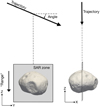 |
Fig. 1 Configuration of the observation for the MARSIS datasets. This case represents a scenario in which MEX is less than 180 km away from Phobos at closest approach. In this configuration, data are only acquired before and after closest approach, and therefore the trajectory is not perpendicular to the range direction. |
2.2 Radar simulations
We performed coherent simulations of MARSIS data using SPRATS (the same toolset used for the SAR synthesis) in order to analyse the data and accurately estimate the error in the geometry. We used ephemerides of MEX and Phobos for our simulations, along with a shape model of Phobos made by Willner et al. (2014). This model is generated using data from HRSC and has a grid spacing of 100 m. We later acquired a more recent and detailed shape model made by Ernst et al. (2023) with a grid spacing of 18 m. We compare the results obtained with both models in Sect. 3.2.
The simulation is based on the facet method and the Huygens-Fresnel principle (Nouvel et al. 2004; Berquin et al. 2015). The contribution from each facet of the surface is summed coherently, which allows us to reproduce the signal as it is sensed by the radar, meaning that we can apply the same SAR processing to simulations and MARSIS data. In doing so, we get rid of the orbital error: unlike real measurements, our simulated radargrams are self-coherent between the simulation and its SAR synthesis, as we use the same trajectory for both. This is not the case for the MARSIS data because the measurements were, by nature, made with the real trajectory, and therefore a different one from that used for the ephemerides.
We measured offsets between the simulations and MARSIS data by superimposing them. We decomposed the offsets coming from the error in the relative position of MEX and Phobos, which can be in three directions:
The range direction is the one radars are most sensitive to. As can be seen in Fig. 2, the shift between simulation and MARSIS data appears to be only in the range direction.
When having an error perpendicular to the range direction in the SAR plane (see Sect. 2.1), the output of the SAR will appear shifted in that direction relative to the simulation. However, given the geometry of the observation, we have poor resolution in that direction.
A shift in the direction of the normal to the SAR zone (across-track from the perspective of MEX) would have little to no impact on the simulation result. Indeed, the magnitude of the offsets are at most of a few kilometres, whereas the distance between MEX and Phobos is between 180 and 250 km. The difference in angle between the true observation and the maximum error will be of 1° at most. At the scale of Phobos, the result is unlikely to be greatly impacted.
We performed sensitivity tests for each of the three directions mentioned above; these show that our sensitivity to the along-track and across-track directions is negligible compared to the range direction. We therefore chose to focus on the range measurements. Also, we did not take into account the orientation of the antenna for this work, as this only influences the power of the echo though the antenna lobe, but has no impact on the range measurement. In Fig. 2, for example, we measure a range offset of 1.12 km between MARSIS and the simulated dataset for orbit n°11634.
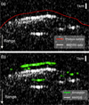 |
Fig. 2 Visualization of the offset of the SAR synthesis of MARSIS dataset n°11634. Panel a: outline of Phobos on top of the data. Panel b: Simulation on top of the same data (in green). |
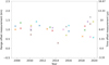 |
Fig. 3 Measurements of the range offsets between MARSIS data and simulations using the Willner et al. (2014) shape model. The corresponding round time offset is shown on the right (round trip). |
3 Offset measurements between MARSIS data and simulations
The SAR synthesis with the chosen SAR zone allows us to locate the radar reflectors in a plane as described in Fig. 1. As mentioned in Sect. 2.2, we only consider the offsets between simulations and MARSIS data in the range direction. For this section, all measurements were made using the Willner et al. (2014) and Ernst et al. (2023) shape models, along with the NOE-4-2020 Phobos orbital kernel (Lainey et al. 2021).
3.1 Offset measurement
For every dataset, we measured the offset that needed to be applied in order to align the MARSIS synthesised image and the simulation. Those offsets are shown in Fig. 2. The shape model is not perfect, and so the simulation does not perfectly align with the MARSIS data on every point of the SAR synthesised signal, making for a 100 m error in the measurement of the range offset.
The range offset measurements are plotted in Fig. 3. When averaging them, we find a value of 1 km, corresponding to an extra delay of 6.67µs in the MARSIS signal. Given that the measurements have been made over the entire surface of Phobos (see Fig. 4), this constant delay is not compatible with a shape model error – its volume would be incorrect – or with an orbital error– the direction of observation is considered random. We therefore consider that the measured average range offset is due to an instrumental delay. We confirm this value in Sect. 4.3. Hereafter, all offset measurements account for instrumental delay.
The corrected measured offsets are shown in Table A.1, and the distribution of offsets has a standard deviation of 400 m. There a various possible sources of this broad distribution; these are discussed in Sect. 4, but we can already rule out instrumental error, because the variations are orders of magnitude below the measured standard deviation. In order to use MARSIS data as control points for the orbit calculation, we provide the actual range measurement between MEX and the surface of Phobos in Table A.2. The issue with this way of presenting the data is that the point that we choose on the radar data is arbitrary. We took the point that is aligned with the middle of MEX’s trajectory and Phobos’ centre of mass as defined by the NOE-4-2020 kernel, which corresponds to the nadir direction in Phobos’ frame. This table also shows the corresponding distance to Phobos’ centre of mass as measured from our comparison with simulations, for both the Willner et al. (2014) and Ernst et al. (2023) shape models. This calculation was made as follows: we calculated the shift needed to be applied to the shape model so that the simulation matches the MARSIS data (taking into account the 6.67 µs instrumental delay), and from that we calculated the distance between MEX and the centre of mass of the shape model. These measurements are more accurate in the sense that we measure the offset by fitting the whole radar profile. The result is that, if there were a localised error on the shape model, it would have less impact on the resulting distance measurement. The use of these measurements for orbital fitting is presented in Appendix B, along with the choice of the time used in both Tables A.1 and A.2 under the columns named ‘Encounter time UTC’.
3.2 The role of the shape model in the offset measurements
One of the first ideas that comes to mind when seeing discrepancies between radar data and simulations is that the shape model is flawed. We performed the measurements with two different shape models: one from Willner et al. (2014) and another from Ernst et al. (2023). By comparing the two in Fig. 5, we observe a shift between them of a few hundreds metres in a particular direction. The difference between the offsets with simulations made using the Willner et al. (2014) and the Ernst et al. (2023) models is shown in Table A.1. We measured the standard deviation and the average of the range measurements taken until 2017 – see Sect. 4 for details on the choice of the date – and find similar values for both (250 m standard deviation and 50 m average using the Willner et al. 2014 model and 300 m standard deviation and 30 m average using the Ernst et al. 2023 one). This shows that while it can improve our measurements, the choice of shape model does not greatly impact their distribution. At several places around Phobos, we can see that some trajectories are overlapping (see Fig. 6). If the range offset were only coming from the shape model, we would measure the same error at the crossing of the two trajectories. However, as shown in Fig. 6, we measure discrepancies of 200–500 meters between any of the crossing trajectories, the same order of magnitude as if we take any pair of datasets until 2017. However, we observe in Fig. 4 that the greater offsets correspond to the more weakly constrained areas of Phobos by the Willner et al. (2014) shape model, meaning that the choice of shape model can have an impact on the local range measurement. These observations show that the shape model can play a minor role in the distribution of offsets, but is not the main source of error.
4 Phobos orbital errors leading to the offset measurements
For dynamical reasons, the most realistic hypothesis when considering an error in the orbit of Phobos is an along-track offset. Indeed, a small error in the determination of the mean motion of the moon will automatically introduce a secular drift over time. To test this hypothesis, we have to estimate the along-track offset that Phobos would need to have in order to create the range offset we measure. In other words, we suppose that the observed range offset is the projection of the Phobos along-track orbital error on the MARSIS line of sight. As the Phobos along-track direction corresponds to the ‘-Y’ direction (see Fig. 7), we apply the following equation in order to convert the range measurements into equivalent Phobos offsets:
 (1)
(1)
where D is the equivalent Phobos along-track offset, δ is the measured range offset, θ is the longitude of the middle point of the dataset, and ( ) is the longitude. See Fig. 7 for more detail. All the MARSIS data were taken for the same Phobos mean anomaly.
The Phobos offset values are shown in Table A.1 and are plotted in Fig. 8. For each measurement, we estimate the confidence interval: the same process is applied to our measurement error of 100 m. These confidence intervals allow us to estimate the impact of a measurement error on the Phobos along-track offset value. With this measurement method, a non-zero range offset measurement made perpendicularly to the Phobos along-track direction corresponds to an infinite Phobos along-track offset. These singularities must be taken into account; this is the reason why the Phobos offset values for orbits 7926 and 18395 are outside the normal range of the others. For those datasets, the trajectory crosses the 180° longitude line, and so the corresponding offset of Phobos along its track (90°/−90° direction on the map) is not meaningful. The evolution of the Phobos along-track error through time using the Willner et al. (2014) shape model and the NOE-4-2020 ephemerides in Fig. 8 presents two clearly distinct regimes. From 2008 to 2016, the measurements are distributed around a constant value of 300 m, with a standard deviation of 500 m; and from 2017, the along-track offset values are distributed along a decreasing line – 2017 being the date of the last measurement set contributing to the kernel.
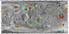 |
Fig. 4 Cylindrical projection of the range offset between the simulation and MARSIS data in colour for the Willner et al. (2014) shape model, and the NOE-4-2020 Phobos kernel. Data are mapped on top of a Viking mosaic taken from Stooke (2015). |
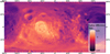 |
Fig. 5 Cylindrical projection of the difference in radius between the shape models made by Ernst et al. (2023) and Willner et al. (2014). |
4.1 Phobos along-track offset values from 2008 to 2016
For the first phase of the measurements, between 2008 and 2016, the dispersion is compatible with the known error on the NOE-4-2020 Phobos ephemeris combined with our 100 m measurement error. The 300 m constant value is the result of the average on the Phobos along-track offsets weighted by the squared error (impact of a 100 m measurement error on Phobos along-track measurement). To estimate the impact of the shape model and the ephemerides used, we performed the same measurements with the Ernst et al. (2023) shape model and the mar097 ephemerides (Jacobson & Lainey 2014). The results are shown in the top half of Table 1, and we notice that the weighted average is closer to zero when using mar097 than when using NOE-4-2020. However, for both datasets, the weighted average value is well below the calculated RMS value shown in the bottom part of the same table. From the comparison of average values alone, one can conclude that the mar097 ephemerides are better than NOE-4-2020 because of the lower average during the first phase of the measurements. However, we note that the standard deviation of the distribution is nearly twice as high when using the mar097 ephemerides than it is with the NOE-4-2020 data. In Fig. 9, we plot the Phobos along-track offset measured with NOE-4-2020 and mar097 through time. In the part from 2008 to 2016, we visualise the difference in standard deviation between the two ephemerides, and note that the mar097 data drift through time by 1–2 km from 2008 to 2016. The measurements made with NOE-4-2020 are therefore more precise than those based on mar097 data. This distribution difference can also be seen in Fig. 10, where we plot the measured Phobos along-track offset with the mar097 ephemerides as a function of the measurements made with the NOE-4-2020 ephemerides, with the colour of the points referring to the year of data acquisition. The first points from 2008 to 2010, in blue, are distributed along a line with a slope of 1. This means that the two ephemerides are similar and that either they use the same control points, or the measured offsets are biased by a common phenomenon: most probably an error on the trajectory of MEX. Then, from 2011 to 2016, the measurements, in green and yellow, are distributed along a line with a slope of 2. The trajectory biases are greater for mar097 than for NOE-4-2020. This difference is coherent with the findings of Lainey et al. (2021), as these authors measure a drift between the two kernels starting from this date.
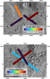 |
Fig. 6 Zoom onto an area where several tracks cross. We can see that orbits crossing each other do not have the same offset value, meaning that the shape model is not the only source of error. Background map taken from Stooke (2015). |
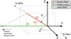 |
Fig. 7 Diagram explaining the geometry of the conversion from range measurements to equivalent Phobos offset. We note that the orbit of Phobos is going in the ‘-Y’ direction, hence the minus sign in Eq. (1). |
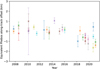 |
Fig. 8 Equivalent Phobos along-track offsets for the measurements using the Willner et al. (2014) shape model and NOE-4-2020 Phobos ephemerides. The colours are for readability only. We note the negative drift of the offset values from 2017. |
Average and standard deviation of Phobos’ along-track offset between 2008 and 2016 measured with different shape models and ephemerides.
4.2 Phobos along-track offset values from 2017 to 2021
When looking at the second half of the Phobos along-track offsets in Fig. 8, from 2017 to 2021, the values are distributed along a decreasing line, from 0 km in 2017 to about −1.5 km in 2021. This decreasing line is due to the fact that the NOE-4-2020 ephemerides are fitted to observations that end in November 2016. It means that from 2017 onwards, the ephemerides are predictive. In absence of astrometric data, it will drift over time. Nevertheless, the measured drift is larger than expected given the estimation of the Phobos ephemeris precision in Lainey et al. (2021), suggesting the existence of a bias in the ephemeris. When comparing the drift using NOE-4-2020 and mar097 in Fig. 9, using the mar097 ephemerides, we measure an offset of about -3km in 2021, which is twice that obtained when using those of NOE-4-2020. On the data measured with the mar097 kernel, we note a constant downwards tendency, which is most likely due to the fact that the latest control point used for the kernel was taken earlier than 2011. This drift speed difference is also visible in Fig. 10, where, from 2017 onwards, NOE-4-2020 and mar097 measure points (shown in orange and red) are distributed along a line with a slope of 2.
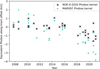 |
Fig. 9 Comparison of the equivalent Phobos along-track offsets for the measurements using NOE-4-2020 and mar097 Phobos ephemerides. The simulations were made using the Willner et al. (2014) shape model. |
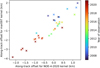 |
Fig. 10 Scatter plot comparing the Phobos along-track offset measured with NOE-4-2020 and mar097 ephemerides. The time of observation is represented in colour. |
4.3 Sensitivity to a global error on the range measurements
In Sect. 3.1, we see that there is an average of 1 km on the range measurements we make, which we chose to subtract from every measurement. To confirm this value, we measured the dispersion of the equivalent Phobos along-track offsets for different deltas applied to all the range measurements. A constant delta was added to all of the range measurements before converting them to an equivalent Phobos along-track offset. By varying this delta from −0.4 km to 0.4km, and measuring the standard deviation on orbits 4814 to 15260 − which are the one where no orbital drift has been observed −, we find that there is a clear minimum around a delta value of 0km (see Fig. 11). This means that the initial guess of substracting 1km from all range measurements is the most coherent solution. Those results were obtained using the NOE-4-2020 Phobos ephemerides and the Willner et al. (2014) shape model. The delta values where the RMS of the Phobos along-track measurements is the lowest for different combinations of shape model and ephemerides is shown in Table 2. On this table, we see that the delta values are close to zero, meaning that our initial guess of substracting 1km from every range measurement is justified. With some kernel – shape model combinations, there is still some error, which could be due to residual terms of error in MARSIS. We will investigate this remaining error in a future study.
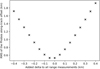 |
Fig. 11 Evolution of the RMS of the Phobos along-track offsets from 2007 to 2016 when adding a constant delay to the range measurements (delta). We note the clear minimum of standard deviation around a delta value of 0 km. The measurements are made with the Ernst et al. (2023) shape model and NOE-4-2020 Phobos kernel. |
Offset to be applied to all datasets in order to have the lowest RMS on the Phobos along-track measurements, depending on the ephemerides and shape model.
5 Conclusions
We measured range offsets between the SAR synthesis of MAR-SIS data and simulations of 35 datasets taken from 2008 to 2021. By estimating the offset that Phobos would need to have along its track in order to produce the measured range offsets, we are able to provide additional astrometric observations to constrain Phobos’ ephemeris. We also provide the raw ranging measurements for them to be used in future ephemerides. These data are available under the DOI : 10.57745/GSMEFN. The precision of our observations depends significantly on the error on the orbit of MEX. Since 2011, the precision on its orbit is of about 200 m. As noted by Lainey et al. (2021), this somewhat large error may be the consequence of the tracking strategy of MEX. Indeed, since 2011, ESA has decreased the amount of tracking data around periapsis, resulting in a poorer constraint on the motion of MEX. This 200 m must be added to our 100 m offset-measurement error, giving a total error of about 225 m on the range observations we provide. With a refinement of MEX’s orbit down to the original 20 m precision, we would be able to provide control points with a precision of about 100 m. We performed those measurements for two different shape models (Willner et al. 2014; Ernst et al. 2023) and two different ephemerides (NOE-4-2020, Lainey et al. 2021 and mar097, Jacobson & Lainey 2014). We determine that the NOE-4-2020 ephemerides produce less dispersion in the orbital error than those of mar097. We also show that with our measurements, we are able to detect the point where the NOE-4-2020 ephemerides start to drift, which corresponds to the last control point used to produce it. This shows that radars are also a useful tool for providing control points for the generation of ephemerides. In order to properly use our measurements to constrain Phobos’ orbit, we also provide the corresponding ranging measurements. Finally, we measured an instrumental delay of 6.6µs for the band III of MARSIS. This delay was previously estimated with MARSIS data while sounding the martian surface Cartacci et al. (2018), but was underestimated because of the difficulty in taking the ionospheric delay into account. The fact that there is no ionosphere between MARSIS and Phobos at the time of sounding makes for a more precise estimation.
A similar approach is proposed for the JuRa radar in the frame of the HERA mission to the Dimorphos asteroid binary system (Herique et al. 2022; Michel et al. 2022) in order to support both the spacecraft and the Dimorphos orbit restitution for operation and science purposes.
Acknowledgements
This project is supported by CNES. Mars Express is an ESA mission. MARSIS instrument has been developed and operated by University of Rome, Jet Propulsion Laboratory Pasadena and Thales Alenia Space under ASI and NASA funding. This research was funded by the Italian Space Agency (ASI) through contract ASI-INAF 2019-21-HH.0. The authors would also like to thank Konrad Willner for his valuable feedback on this work, along with the anonymous reviewer whose remarks helped improve this paper.
Appendix A Offset measurements data
This appendix is composed of two tables, in which one can find the reference of the datasets that were used in this study, along with the measured offsets for every one of them. These tables are showed on the following two pages.
Range offset measurements for Willner et al. (2014) and Ernst et al. (2023) shape models. The corresponding offsets of Phobos along its track are calculated using the method discussed in section 4. The longitude and latitude values are taken for the central point of the trajectory. The time reference is also taken for the central point, and is discussed in more detail in Appendix B.
Distance between MEX and the surface measured by MARSIS. These values represent the distance to the point of Phobos that is equidistant from the centres of mass of MEX and Phobos. For an easier use of the data, we can convert those measurements into distances to the centre of mass for both the Willner et al. (2014) and Ernst et al. (2023) shape models using the offset between simulations and MARSIS data (see section 3.1 for more detail). The longitudes and latitudes are taken for the central point of the trajectory for each dataset, and so is the time. The precise moment chosen as time reference is discussed in Appendix B.
Appendix B Using MARSIS ranging measurement for orbital fitting
In this Appendix, we present our proposed method of how to consider the MARSIS ranging measurements when solving for physical parameters with an orbital model of Phobos. As the general method for orbit fitting of natural satellites was already described in Lainey (2016), here we simply describe how the observation function should be constructed.
Let r and s being the Phobos and Mars Express position vectors in a Mars-centric J2000 frame, respectively, as schematised in Figure B.1. The Phobos position as seen from Mars Express at the time t0 of the ranging observation can be approximated by p = r(t0 + τ) − s(t0 + τ), where τ is the one-way light time correction between Phobos and Mars Express. In practice, the time furnished in the MARSIS data is the Rx window opening time, labelled tRx in Figure B.1.
Hence, the difference between the measured and computed ranging p = |p| can be expressed as
 (B.1)
(B.1)
where the superscript O and C refer to ‘observed’ and ‘computed’, while Δcl stands for the correction to be applied to the physical parameters to be retrieved from the fit (initial state coordinate, mass, etc.).
As sC has to be independent from cl, we immediately get
 (B.2)
(B.2)
In practice, the partial  is obtained from the integration of the variational equations (see Lainey 2016 for details).
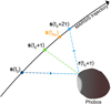 |
Fig. B.1 Schematic position of MARSIS at each step of the sounding. The date expressed in the MARSIS data is tRx, and the reference we chose is t0 + τ. |
References
- Acton, C. H. 1996, Planet. Space Sci., 44, 65 [Google Scholar]
- Berquin, Y., Herique, A., Kofman, W., & Heggy, E. 2015, Rad. Sci., 50, 1097 [NASA ADS] [CrossRef] [Google Scholar]
- Cartacci, M., Sánchez-Cano, B., Orosei, R., et al. 2018, Icarus, 299, 396 [NASA ADS] [CrossRef] [Google Scholar]
- Cicchetti, A., Nenna, C., Plaut, J., et al. 2017, Adv. Space Res., 60, 2289 [CrossRef] [Google Scholar]
- Cicchetti, A., Nenna, C., Cartacci, M., Noschese, R., & Orosei, R. 2023, INAF Technical Reports - Rapporti Tecnici INAF, 259, http://hdl.handle.net/20.500.12386/33358 [Google Scholar]
- Ernst, C. M., Daly, R. T., Gaskell, R. W., et al. 2023, Earth Planets Space, 75, 103 [NASA ADS] [CrossRef] [Google Scholar]
- Gassot, O., Herique, A., Rogez, Y., et al. 2020, in 2020 IEEE Radar Conference RadarConf20, Florence, Italy: IEEE, 1 [Google Scholar]
- Herique, A., Plettemeier, D., & Kofman, W. 2022, JuRa: the Juventas Radar on Hera to fathom Didymoon, Technical Report EPSC2022-487, Copernicus Meetings, conference Name: EPSC2022 [Google Scholar]
- Jacobson, R., & Lainey, V. 2014, Planet. Space Sci., 102, 35 [CrossRef] [Google Scholar]
- Jordan, R., Picardi, G., Plaut, J., et al. 2009, Planet. Space Sci., 57, 1975 [NASA ADS] [CrossRef] [Google Scholar]
- Lainey, V. 2016, Celest. Mech. Dyn. Astron., 126, 145 [NASA ADS] [CrossRef] [Google Scholar]
- Lainey, V., Pasewaldt, A., Robert, V., et al. 2021, A&A, 650, A64 [NASA ADS] [CrossRef] [EDP Sciences] [Google Scholar]
- Michel, P., Küppers, M., Bagatin, A. C., et al. 2022, Planet. Sci. J., 3, 160 [NASA ADS] [CrossRef] [Google Scholar]
- Nouvel, J.-F., Herique, A., Kofman, W., & Safaeinili, A. 2004, Rad. Sci., 39, RS1013 [NASA ADS] [CrossRef] [Google Scholar]
- Pascu, D., Erard, S., Thuillot, W., & Lainey, V. 2014, Planet. Space Sci., 102, 2 [Google Scholar]
- Picardi, G., Plaut, J. J., Biccari, D., et al. 2005, Science, 310, 1925 [NASA ADS] [CrossRef] [Google Scholar]
- Pou, L., Nimmo, F., Lognonné, P., et al. 2021, Earth Space Sci., 8, e2021EA001669 [CrossRef] [Google Scholar]
- Stooke, P. 2015, NASA Planetary Data System, Small Bodies Maps V3.0. MULTI-SA-MULTI-6-STOOKEMAPS-V3.0 [Google Scholar]
- Willner, K., Shi, X., & Oberst, J. 2014, Planet. Space Sci., 102, 51 [Google Scholar]
- Ziese, R., & Willner, K. 2018, A&A, 614, A15 [EDP Sciences] [Google Scholar]
All Tables
Average and standard deviation of Phobos’ along-track offset between 2008 and 2016 measured with different shape models and ephemerides.
Offset to be applied to all datasets in order to have the lowest RMS on the Phobos along-track measurements, depending on the ephemerides and shape model.
Range offset measurements for Willner et al. (2014) and Ernst et al. (2023) shape models. The corresponding offsets of Phobos along its track are calculated using the method discussed in section 4. The longitude and latitude values are taken for the central point of the trajectory. The time reference is also taken for the central point, and is discussed in more detail in Appendix B.
Distance between MEX and the surface measured by MARSIS. These values represent the distance to the point of Phobos that is equidistant from the centres of mass of MEX and Phobos. For an easier use of the data, we can convert those measurements into distances to the centre of mass for both the Willner et al. (2014) and Ernst et al. (2023) shape models using the offset between simulations and MARSIS data (see section 3.1 for more detail). The longitudes and latitudes are taken for the central point of the trajectory for each dataset, and so is the time. The precise moment chosen as time reference is discussed in Appendix B.
All Figures
|
Fig. 1 Configuration of the observation for the MARSIS datasets. This case represents a scenario in which MEX is less than 180 km away from Phobos at closest approach. In this configuration, data are only acquired before and after closest approach, and therefore the trajectory is not perpendicular to the range direction. |
| In the text | |
|
Fig. 2 Visualization of the offset of the SAR synthesis of MARSIS dataset n°11634. Panel a: outline of Phobos on top of the data. Panel b: Simulation on top of the same data (in green). |
| In the text | |
|
Fig. 3 Measurements of the range offsets between MARSIS data and simulations using the Willner et al. (2014) shape model. The corresponding round time offset is shown on the right (round trip). |
| In the text | |
|
Fig. 4 Cylindrical projection of the range offset between the simulation and MARSIS data in colour for the Willner et al. (2014) shape model, and the NOE-4-2020 Phobos kernel. Data are mapped on top of a Viking mosaic taken from Stooke (2015). |
| In the text | |
|
Fig. 5 Cylindrical projection of the difference in radius between the shape models made by Ernst et al. (2023) and Willner et al. (2014). |
| In the text | |
|
Fig. 6 Zoom onto an area where several tracks cross. We can see that orbits crossing each other do not have the same offset value, meaning that the shape model is not the only source of error. Background map taken from Stooke (2015). |
| In the text | |
|
Fig. 7 Diagram explaining the geometry of the conversion from range measurements to equivalent Phobos offset. We note that the orbit of Phobos is going in the ‘-Y’ direction, hence the minus sign in Eq. (1). |
| In the text | |
|
Fig. 8 Equivalent Phobos along-track offsets for the measurements using the Willner et al. (2014) shape model and NOE-4-2020 Phobos ephemerides. The colours are for readability only. We note the negative drift of the offset values from 2017. |
| In the text | |
|
Fig. 9 Comparison of the equivalent Phobos along-track offsets for the measurements using NOE-4-2020 and mar097 Phobos ephemerides. The simulations were made using the Willner et al. (2014) shape model. |
| In the text | |
|
Fig. 10 Scatter plot comparing the Phobos along-track offset measured with NOE-4-2020 and mar097 ephemerides. The time of observation is represented in colour. |
| In the text | |
|
Fig. 11 Evolution of the RMS of the Phobos along-track offsets from 2007 to 2016 when adding a constant delay to the range measurements (delta). We note the clear minimum of standard deviation around a delta value of 0 km. The measurements are made with the Ernst et al. (2023) shape model and NOE-4-2020 Phobos kernel. |
| In the text | |
|
Fig. B.1 Schematic position of MARSIS at each step of the sounding. The date expressed in the MARSIS data is tRx, and the reference we chose is t0 + τ. |
| In the text | |
Current usage metrics show cumulative count of Article Views (full-text article views including HTML views, PDF and ePub downloads, according to the available data) and Abstracts Views on Vision4Press platform.
Data correspond to usage on the plateform after 2015. The current usage metrics is available 48-96 hours after online publication and is updated daily on week days.
Initial download of the metrics may take a while.