| Issue |
A&A
Volume 675, July 2023
BeyondPlanck: end-to-end Bayesian analysis of Planck LFI
|
|
|---|---|---|
| Article Number | A2 | |
| Number of page(s) | 11 | |
| Section | Numerical methods and codes | |
| DOI | https://doi.org/10.1051/0004-6361/202142799 | |
| Published online | 28 June 2023 | |
BEYONDPLANCK
II. CMB mapmaking through Gibbs sampling
1
Department of Physics, University of Helsinki, Gustaf Hällströmin katu 2, Helsinki, Finland
e-mail: This email address is being protected from spambots. You need JavaScript enabled to view it.
2
Helsinki Institute of Physics, University of Helsinki, Gustaf Hällströmin katu 2, Helsinki, Finland
3
Institute of Theoretical Astrophysics, University of Oslo, Blindern, Oslo, Norway
4
Dipartimento di Fisica, Università degli Studi di Milano, Via Celoria, 16, Milano, Italy
5
INAF-IASF Milano, Via E. Bassini 15, Milano, Italy
6
INFN, Sezione di Milano, Via Celoria 16, Milano, Italy
7
INAF – Osservatorio Astronomico di Trieste, Via G. B. Tiepolo 11, Trieste, Italy
8
Planetek Hellas, Leoforos Kifisias 44, Marousi 151 25, Greece
9
Department of Astrophysical Sciences, Princeton University, Princeton, NJ, 08544, USA
10
Jet Propulsion Laboratory, California Institute of Technology, 4800 Oak Grove Drive, Pasadena, CA, USA
11
Computational Cosmology Center, Lawrence Berkeley National Laboratory, Berkeley, CA, USA
12
Haverford College Astronomy Department, 370 Lancaster Avenue, Haverford, PA, USA
13
Max-Planck-Institut für Astrophysik, Karl-Schwarzschild-Str. 1, 85741 Garching, Germany
14
Dipartimento di Fisica, Università degli Studi di Trieste, Via A. Valerio 2, Trieste, Italy
Received:
1
December
2021
Accepted:
19
March
2022
Abstract
We present a Gibbs sampling solution to the mapmaking problem for cosmic microwave background (CMB) measurements that builds on existing destriping methodology. Gibbs sampling breaks the computationally heavy destriping problem into two separate steps: noise filtering and map binning. Considered as two separate steps, both are computationally much cheaper than solving the combined problem. This provides a huge performance benefit as compared to traditional methods and it allows us, for the first time, to bring the destriping baseline length to a single sample. Here, we applied the Gibbs procedure to simulated Planck 30 GHz data. We find that gaps in the time-ordered data are handled efficiently by filling them in with simulated noise as part of the Gibbs process. The Gibbs procedure yields a chain of map samples, from which we are able to compute the posterior mean as a best-estimate map. The variation in the chain provides information on the correlated residual noise, without the need to construct a full noise covariance matrix. However, if only a single maximum-likelihood frequency map estimate is required, we find that traditional conjugate gradient solvers converge much faster than a Gibbs sampler in terms of the total number of iterations. The conceptual advantages of the Gibbs sampling approach lies in statistically well-defined error propagation and systematic error correction. This methodology thus forms the conceptual basis for the mapmaking algorithm employed in the BEYONDPLANCK framework, which implements the first end-to-end Bayesian analysis pipeline for CMB observations.
Key words: cosmic background radiation / methods: numerical / methods: data analysis
© The Authors 2023
 Open Access article, published by EDP Sciences, under the terms of the Creative Commons Attribution License (https://creativecommons.org/licenses/by/4.0), which permits unrestricted use, distribution, and reproduction in any medium, provided the original work is properly cited.
This article is published in open access under the Subscribe to Open model. This email address is being protected from spambots. You need JavaScript enabled to view it. to support open access publication.
1. Introduction
The removal of correlated 1/f noise generated by detectors is a crucial step in the data processing chain for cosmic microwave background (CMB) measurements. Noise removal is most commonly done jointly with mapmaking and a number of different methods have been developed for this purpose. For reviews of different methods applied to Planck, we refer to Poutanen et al. (2006), Ashdown et al. (2007a,b, 2009), and references therein. For a closely related discussion of Bayesian noise estimation with time-ordered CMB data, we refer to Wehus et al. (2012).
Conventional mapmaking produces (as its initial output) pixelized sky maps of CMB temperature and polarization at a given frequency. These pixelized sky maps then serve as input for the separation of astrophysical components (e.g., Planck Collaboration IV 2020), including the CMB, and further for power spectrum estimation (e.g., Planck Collaboration V 2020). As input, mapmaking takes the calibrated time-ordered information (TOI) data stream, together with corresponding detector pointing information.
The generalized least-squares methods (GLS) are aimed at finding the map, m, that maximizes the likelihood of the data P(d ∣ m), where the likelihood depends on an assumed known noise spectrum. Another widely used approach is the destriping technique (Burigana et al. 1999; Delabrouille 1998; Maino et al. 1999, 2002; Keihänen et al. 2004, 2005, 2010; Sutton et al. 2009; Kurki-Suonio et al. 2009), where the correlated noise component is modelled as a sequence of offsets, whose amplitudes are then solved for through maximum likelihood analysis and then subtracted from the timeline.
Conventional mapmaking, whether GLS or destriping, is a memory-intensive data processing step, since it requires that all the detector pointing information for the data set is kept in memory simultaneously. This follows from the coupling between two signal components with very different characteristics: the sky signal (represented by a map) is dependent on the detector’s pointing on the sky, while the noise component is correlated in the time domain but independent of where the detector is pointing.
In this work, we examine the possibility of solving the mapmaking and noise removal problem through a Gibbs sampling technique. Gibbs sampling breaks the computationally heavy mapmaking problem into two separate steps: noise removal and construction of the sky signal from noise-cleaned TOI. Considered as isolated steps, both are much simpler than the combined mapmaking procedure. As a test case. we use simulated Planck LFI data in the context of the BEYONDPLANCK project. For an introduction to Gibbs sampling theory and for an overview of the BEYONDPLANCK project, we refer the reader to the first paper of this series, BeyondPlanck Collaboration (2023).
A great benefit of the proposed procedure is that the noise removal step can be carried out separately for each Planck pointing period, reducing the memory requirement tremendously, as compared to conventional mapmaking methods. Second, in the absence of data flagging and Galactic masking, the noise removal step reduces into a simple fast Fourier transform (FFT) filtering operation, in which case the computational cost of noise removal is equivalent to only two FFTs of the full TOI. Flagging, however, breaks the stationarity of the data and we examine two alternative solutions to this problem: the filling of gaps with a Gibbs technique and exactly solving the non-stationary filtering problem. As a consequence of these two facts, we are for the first time able to reduce the length of the destriping baseline to one single TOI sample, with a significantly lower combined computational cost than traditional approaches.
As a byproduct, the Gibbs mapmaking process also yields an estimate of the residual noise in the output products in the form of a discrete set of samples that accounts for both white and residual correlated noise, without the need to compute a noise covariance matrix. The computational cost of running a full Gibbs chain, such as that described in this paper, must therefore be compared to the cost of generating a full ensemble of end-to-end simulations or the cost of evaluating a dense noise covariance matrix in a traditional pipeline.
The main focus of this paper is on the noise removal step. For demonstration purposes, we combine noise removal with a simple pixel-based mapmaking procedure. For this purpose we have written a stand-alone test code, which allows us to study the mapmaking step in separation, independently from the Commander code (Eriksen et al. 2008; Galloway et al. 2023) that forms the basis for the BEYONDPLANCK processing. The great potential of the method, however, lies in a scenario where noise removal is combined within the Gibbs framework with modeling of the sky signal and instrument effects, which is the main overall goal of the BEYONDPLANCK project. The methodology presented in this paper forms the conceptual basis for the mapmaking algorithm employed in the BEYONDPLANCK framework, which implements the first end-to-end Bayesian analysis pipeline for CMB observations (BeyondPlanck Collaboration 2023; Galloway et al. 2023).
2. Methodology
2.1. Gibbs sampling procedure
We consider a time-ordered data stream from one detector of a Planck-like CMB experiment, which may be modelled as
 (1)
(1)
Here, P is the pointing matrix, which encodes the scanning strategy and the detector’s response to temperature and polarization, and m is the pixelized sky map, which includes temperature and polarization components in the form of I, Q, U Stokes components. Formally, P is a large matrix (Nt, 3Np), where Nt is the number of samples in the time-ordered data stream and Np is the number of pixels in the sky map. In the place of Pm we could have other sky models, for instance, a harmonic representation of the sky, or a parametrized foreground model. In this work, we do not pursue these possibilities further and instead we assume the simple pixelized sky model.
The instrument noise of Planck LFI radiometers is well approximated as Gaussian distributed (Bersanelli et al. 2010). The noise stream can be divided into two components: correlated 1/f noise and uncorrelated white noise. In the spirit of destriping, we model the correlated noise component as a sequence of constant offsets, or “baselines” of fixed length Na. We write the noise term as
 (2)
(2)
where a represents the baseline amplitudes, and F is a matrix which formally projects them into a full data stream. With a baseline length of Na, each column of F has the value 1 along Na adjacent elements, and the value 0 elsewhere. In the extreme limit in which the baseline length equals one sample, F becomes a unity matrix and can be dropped from the equations. The last term, n, represents white noise.
We denote the covariance matrices of a and n by Ca and Cw, respectively, where Cw is diagonal (but not necessarily uniform), and Ca is the covariance of the noise baseline amplitudes. If the noise is stationary, the latter is band-diagonal to a good approximation, and can be represented as a filter in Fourier domain. If the baseline length equals one TOI sample (Na = 1), Ca becomes equal to the time-domain covariance of the 1/f noise component. The construction of the covariance in the general case of Na > 1 is presented in Keihänen et al. (2010); in this work we will assume Na = 1. In the following, both covariance matrices are assumed to be known a priori. Estimating the noise properties from the data itself (as part of the Gibbs sampling process) is addressed by Ihle et al. (2023).
We now proceed to write out the posterior distribution, P(m, a ∣ y, Cw, Ca), for the (a, m) model, given some TOI data stream, y, and assumed known noise properties. This is the posterior distribution we eventually want to sample by using Gibbs sampling technique, and may, according to Bayes’ theorem, be written as
 (3)
(3)
Here, we have assumed that a are m are statistically independent, and we include Ca and Cw explicitly only in factors for which the conditional in question actually depends on them. The denominator P(y) is an overall normalization factor and can be ignored, since the methods we use for drawing samples from the likelihood are insensitive to the normalization. Furthermore, we assume a uniform prior for the sky map m, P(m)=1, such that
 (4)
(4)
The first factor on the right is the probability of observing a data stream, y, for given realization of correlated noise, a, and for a given sky map, m. With both a and m fixed, the only difference between the model and the data comes from white noise. We obtain this likelihood from the white noise distribution, which is assumed to be Gaussian with covariance Cw,
 (5)
(5)
The second distribution on the right-hand side of Eq. (4) represents a prior on a, namely, the probability of obtaining a given realization of correlated noise in the abscence of actual measurements. As is customary in Planck mapmaking, we assume that the correlated noise component also is Gaussian distributed, such that
 (6)
(6)
The conventional destriping procedure finds the combination (a, m) that maximizes the posterior distribution in Eq. (4). Equating the derivative of this expression with respect to (a, m) to zero leads to a large linear system, which can be solved by conjugate gradient iteration (see, e.g., Keihänen et al. 2010).
In this paper, we instead proceed to use Gibbs sampling to sample from the distribution in Eq. (4). One full Gibbs sampling step consists of two substeps, in each of which one of the two parameters m, a is kept fixed, and the other is drawn from the corresponding conditional distribution,
 (7)
(7)
We use the semicolon to separated sampling parameters, which are however considered constant in the current sampling step, from parameters not sampled. Here, the symbol “←” indicates drawing a sample from the distribution on the right-hand side. Let us now look at these two substeps more closely:
1. For a given data stream, y, and noise baselines, a, we update the sky map, m, by drawing a sample from the Gaussian distribution:
 (8)
(8)
where y′ = y − Fa is the data stream from which we have subtracted the current a sample. Thus, y′ represents the current estimate of the noise-cleaned TOI stream.
2. For given data stream, y, and sky, m, we update the baseline vector a′ by drawing a sample from the distribution:
 (9)
(9)
where now y′″ = y − Pm is a data stream from which we have subtracted the current m sample. Thus, y′″ represents the current estimate of the noise-only TOI stream.
The outcome from the sampling procedure is a chain of m and a samples, with their distribution sampling the combined likelihood of Eq. (4).
The conditional distributions in Eqs. (8) and (9) are both multivariate Gaussian distributions, from which samples may be drawn efficiently using standard methods (see, e.g., Appendix A in BeyondPlanck Collaboration 2023 and references therein). In the following, we briefly review the main steps for convenient reference purposes.
Consider a Gaussian distribution for a stochastic variable x,
 (10)
(10)
where y represents data (observations); A is some linear operator that connects the unknown x to the data; Cn is the noise covariance, which may or may not be diagonal; and Cx is an optional covariance matrix for the prior of x. The value of x that maximizes the likelihood is readily found to be:
 (11)
(11)
Rather than finding the maximum-likelihood solution, we now want to draw a random sample of the distribution in Eq. (10). This can be done by solving a linear system similar to that of Eq. (11), but with a modified right-hand side b, as follows:
 (12)
(12)
Here, ω1 and ω2 are two vectors of random numbers drawn from a normalized Gaussian distribution N(0, I). The first vector has length equal to that of the data stream, y, and the second one to that of x.
We go on to apply this to our mapmaking problem. We take turns in drawing samples from the distributions of Eqs. (8) and (9). We end up with the following two-step procedure. Starting from sample (m, a), we update the parameters as follows.
![Mathematical equation: $$ \begin{aligned} \boldsymbol{m}^\prime = (\mathtt P ^T \mathtt C _{ w}^{-1}\mathtt P )^{-1} [\mathtt P ^T \mathtt C _{ w}^{-1} (\boldsymbol{y}-\mathtt F \boldsymbol{a}) + \mathtt C _{ w}^{-1/2}\boldsymbol{\omega }_1]. \end{aligned} $$](/articles/aa/full_html/2023/07/aa42799-21/aa42799-21-eq13.gif)
To draw one pair of samples we thus need three independent Gaussian random vectors, ω1, ω2, and ω3. Equations (13) and (14) summarize our Gibbs mapmaking algorithm.
2.2. Assumptions and optimization
The above discussion is general, and few assumptions regarding the experiment in question are made. However, to make the formalism more practical in terms of computer code implementation, we make a few assumptions that are familiar from the conventional Planck data processing pipeline:
First, we assume that all signal recorded by a detector at a time comes from the pixel where the beam center falls. With this assumption, the pointing matrix P is sparse, with three nonzero elements on each row, corresponding to three Stokes components of one pixel. In doing so, we are effectively regarding the beam smoothing as a property of the sky itself, an assumption which is strictly valid only for symmetric beams. The BEYONDPLANCK pipeline applies to the maps a beam leakage correction, as described by Svalheim et al. (2023).
The precise treatment of an asymmetric beam requires a full beam deconvolution. The task of beam deconvolution is simplified by the Planck scanning strategy, where multiple rotations fall on the same scanning ring. Full beam deconvolution has been shown to be feasible for Planck-like data sets (Keihänen & Reinecke 2012), however, this is beyond the scope of this work. Beam deconvolution in the context of BEYONDPLANCK is discussed further in Suur-Uski et al. (in prep.).
Second, we do not correct for bandpass effects and we assume that all detectors see the same sky. Third, the detector noise is uncorrelated between pointing periods. Furthermore, correlated noise within a pointing period is Gaussian and stationary. Finally, the white noise component, by definition, is uncorrelated from sample to sample, but not necessarily with constant variance. The covariance Cw is thus diagonal, but the values of the diagonal elements are allowed to vary. In the following we make the further simplifying assumption that the variance stays constant within one pointing period. However, we do allow for the possibility that some of the samples are discarded from the analysis by setting  .
.
Based on these assumptions, the coupling matrix  is block-diagonal and consists of a 3 × 3 block per pixel that may be easily inverted. The map sampling step of Eq. (13) represents a simple binning operation, where the noise-cleaned TOI samples are coadded into pixels as given by the pointing matrix P, and the resulting map is normalized with the corresponding 3 × 3 matrix.
The noise sampling step can be carried out independently for each pointing period, which has an average length of about 40 min. This leads to a significant memory saving when compared to full mapmaking, and for the first time we can bring the baseline length down to one single sample. At this extreme limit F reduces to the identity matrix, F = I, and the noise sampling step of Eq. (14) is simplified to:
 (15)
(15)
and
 (16)
(16)
Here the term  represents the operation of applying the noise filter to a sequence of Gaussian random numbers. Since Ca is stationary, this can be carried out efficiently with FFT technique.
To increase the efficiency of the FFT operations, it is useful to pad the data to a suitable FFT length. In this paper, we have chosen the following procedure to deal with data ends: to reduce boundary effects, we first subtract the mean of the data (over unflagged samples) and only then do we pad the data with zeroes to a suitable FFT length. We then carry out the FFT operation, apply the relevant filter, perform the inverse FFT; cut off the padded region, and add back the original offset.
2.3. Flagging and masking
As mentioned regarding Eq. (16),  represents a stationary filter. However, the presence of missing observations makes the full coupling matrix
  non-stationary. The two most common causes for missing observations are glitches in the data collection and the application of an analysis mask that excludes bright foreground regions on the sky, which is useful for preventing striping along the scanning path of the instrument.
The most convenient way of implementing masking is by formally setting the white noise level to infinity for the discarded samples, or, equivalently, to  . The computational price for this is that Eq. (16) can no longer be treated as a strict Fourier filter. The system can still be solved through conjugate gradient iteration, but this is significantly slower than solving the stationary system. A faster, but approximate, solution is to fill the gaps with a simulated data. We consider both options more closely in the following.
2.3.1. Solving the non-stationary system
We first consider the exact solution of the non-stationary system in Eq. (16), where  in the flagged part of the data. Let us for convenience define:
 (17)
(17)
and M to be a stationary version of the same, with flags appropriately omitted,
 (18)
(18)
If only a small fraction of samples are flagged, we have:
 (19)
(19)
Conjugate gradient iteration can be sped up significantly with a properly chosen preconditioner matrix. In our case, M represents a natural choice for a preconditioner. However, even with preconditioning, full convergence typically requires 40−50 iteration steps, which becomes computationally prohibitive when this algorithm is repeated within every Gibbs loop.
Fortunately, we can speed up the procedure significantly by reformulating the problem as follows. We first symbolically write the right-hand side of Eq. (16) in the form:
 (20)
(20)
Second, we define:
 (21)
(21)
to be the deviation from the constant white noise variance in Cw. Explicitly, D is a diagonal matrix with zero on the diagonal for the non-flagged samples, and 1/σ2 for the flagged ones. We denote by the number of flagged samples on the pointing period by Nf, and the total number of samples by Ns. Typically, only a small fraction of samples are flagged and, thus, Nf is shown to be much smaller than Ns. We then decompose D into D = UδUT in eigenmode, where δ is a diagonal matrix of size (Nf, Nf) with 1/σ2 on the diagonal. The matrix U has size (Ns, Nf), with each column of U corresponding to one flagged sample and containing one nonzero (equal to one) element marking its position on the data stream.
Using this notation we have:
 (22)
(22)
Using the well-known Woodbury matrix identity we can re-write the matrix inverse into the form:
 (23)
(23)
The solution of Eq. (16) therefore becomes
 (24)
(24)
where we have written δ−1 = σ2I. This expression conforms to the format of Eq. (20) and is the solution we were aiming at.
The vector a′ can now be computed efficiently from Eq. (24). The first term, M−1b, represents the operation of applying the stationary filter of M to the right-hand side b, and can be carried out efficiently by FFT techniques. The rest represents a correction that takes care of flagging. Working from right to left, the matrix UT represents the trivial operation of picking the flagged samples from a full TOI, and concatenating them into a vector of length Nf. The middle matrix inversion must still be carried out using conjugate gradient iteration, but the system is now much smaller than the original one. Finally, the matrix U represents the operation of inserting the Nf values of its target vector into a full-size TOI, in the positions of the flagged samples. We find that the solution of Eq. (24) requires only 5−6 iteration steps for convergence, to be contrasted with 40−50 steps required for the original system to converge.
2.3.2. Gap filling
As efficient as this procedure may be, it involves a computational cost that is five to six times higher when compared to a case where no flagging is applied. Thus, in the following, we present an alternative way of handling the flagged data sections: we fill them with a noise realization, as part of the overall Gibbs sampling procedure. We note that similar gap filling techniques have been routinely used by a long history of previous CMB experiments, including Planck LFI (e.g., Planck Collaboration II 2014) and in the following, we discuss both the exact and approximate solutions to this problem.
First, we introduce the white noise component w in the flagged section as a new explicit Gibbs variable to be sampled over. The original noise sampling step,
 (25)
(25)
is therefore replaced by a two-step procedure
 (26)
(26)
The first step consists of generating a white noise sample for all flagged TOI segments, which is simply equivalent to drawing a random realization from the Gaussian distribution with variance Cw = σ2I. The second step represents the usual sampling operation of Eqs. (15) and (16), but this time, for a full data stream where the gaps are filled and, consequently, the white noise covariance Cw is uniform.
The remaining question considers what should go in place of y − Pm′ in Eq. (15)? This vector represents the current best estimate of the noise stream, including both correlated and white noise. In the non-flagged data section, it is therefore raw data minus the sky estimate, as usual. In the flagged section, where no information is available from the data regarding y, it is given by the correlated noise TOI, a, from the preceding Gibbs iteration plus the white noise realization, w, that had just been generated, With the gaps filled in this manner, the calculation of Eq. (16) can be solved with FFT technique without CG iteration and, thus, the overall algorithm becomes very fast.
This solution has two potential disadvantages compared to the original solution that are worth keeping in mind. The first is a longer overall Monte Carlo correlation length, which arises from the fact that we are now conditionally sampling the correlated and white noise terms separately, which is always less efficient than sampling them jointly. The second disadvantage is the fact that this method increases the overall memory requirements, since the correlated noise TOI for the flagged section also have to be stored in memory between two consecutive Gibbs iterations. We test both solutions with simulations.
3. Simulations
We characterized and validated the algorithms described above using controlled simulated data. Specifically, we created a set of simulated time-ordered data using the Level-S simulation software (Reinecke et al. 2006). We chose to focus on the Planck LFI 30 GHz channel, since the data set for this particular channel is the smallest of the Planck channels in terms of data volume and, therefore, it also has the fastest turnaround time. The simulated data span the full Planck LFI mission, namely, four years of observations.
The simulated data contain time streams for CMB, foregrounds, and noise. The steps of this process are as follows. We simulate each component separately and use the sum of all time streams as an input to the Gibbs mapmaker. The CMB signal is simulated based on theoretical angular power spectra, while the foreground model is adopted from a preliminary BEYONDPLANCK analysis, taking into account radiometer-specific beam and bandpass responses. Both CMB and foreground simulations contain real Planck main and intermediate beams, as described by Planck Collaboration IV (2016). We use conviqt (Prézeau & Reinecke 2010) and multimod tools from the PlanckLevel-S package to convolve the sky with the beam, and to scan a time-ordered data stream from the input sky according to the detector pointing. The noise TOI is simulated on the basis of realistic noise parameters, as described by Planck Collaboration II (2016), and generated with multimod.
The Planck LFI detector pointing is regenerated with Level-S and has been confirmed to agree well with the real Planck LFI pointing. We use actual Planck LFI flags to discard flagged samples. This includes the so-called repointing periods, during which the spin axis of the satellite is moving. Additionally, we use a processing mask described by BeyondPlanck Collaboration (2023) to mask out regions with strong gradients.
In addition, we generate a set of 101 noise realizations by creating a noise TOD with Level-S and calculating corresponding maps with Madam. We use this set of maps to study potential noise biases. The noise realization used in the main validation work of the Gibbs sampler is the first noise MC sample. Hence we have a total of 102 noise realizations.
4. Results
We then ran the Gibbs sampling mapmaking algorithm described in Sect. 2 on the simulation data described in Sect. 3. As already mentioned, we used a test code for this purpose that is independent of the Commander code that is employed for the full BEYONDPLANCK analysis, as summarized by BeyondPlanck Collaboration (2023). This allows us to examine the mapmaking problem in isolation and also to try out different approaches with a faster turnaround time. The test code implements the Gibbs sampling mapmaking procedure, as presented in Sect. 2, without any component separation step. The output maps thus contain both the CMB and foreground signal, and represent traditional frequency maps, rather than astrophysical component maps. We implemented the following steps, running the code both in “sampling mode” and in “maximum-likelihood mode.” In the sampling mode, the code performs full Gibbs sampling, and draws samples from the combined baseline-plus-map posterior distribution. In the maximum-likelihood mode, the fluctuation terms that involve ω1, ω2, and ω3 in Eqs. (13) and (14) are omitted, with the effect that the algorithm performs a (computationally very inefficient) steepest-descent search towards the maximum-likelihood solution.
In the following, we refer to the posterior mean map, as evaluated from the mean of the ensemble of posterior samples, as the “Gibbs map”, with a burn-in period appropriately excluded. Thus, the Gibbs map represents a single-point estimate of the true map. In contrast, the “maximum-likelihood map” refers to the last sample of a chain with the sampling terms disabled.
Unless stated otherwise, we fill the gaps as described in Sect. 2.3.2, using the previous correlated noise sample as a baseline. In the noise-sampling step, we mask the Galactic region to reduce leakage of strong foreground signal into polarization. The mask is applied only in the noise sampling step, while in the map-binning step, all data are included, such that a full-sky map is produced as output. We briefly discuss the other option, exact solution of the non-stationary system, in Sect. 4.3.
Because we are working with simulated data, we know exactly what the true sky signal should be. As a reference, we therefore construct a map from the pure CMB-plus-foreground time stream, and exclude both correlated and white noise. We refer to this ideal map as the “noise-free map”, which represents the map we would obtain in the absence of instrumental noise. The difference between the Gibbs estimates and this map provides a measure of residual noise in the former.
We constructed another validation reference by running the Madam mapmaking code on the same simulated data. Both Madam and the new Gibbs sampler, when run in the maximum-likelihood mode, essentially solve the same likelihood problem, however, using different methods of implementation. We thus expect the results to be very close, if not identical. Small differences may arise due different baseline lengths or from different implementation of the noise filter, or simply from different convergence properties. In particular, since a Gibbs sampler only allow changes along coordinate directions, we expect this approach to converge much slower towards the maximum-likelihood solution than a conjugate gradient solver like Madam. We note, however, that the Gibbs sampling approach will normally not be used in the maximum-likelihood mode, but rather as a sampler within a more complete analysis framework.
4.1. Pixel space
We begin by inspecting the maps visually. Figure 1 shows the unnormalized χ2 difference, computed as the squared difference between the noise-free map and a map from the Gibbs chain, as a function of the sample number. For each map, we first subtract the mean of I to remove arbitrary map offsets. This applies for all maps in this paper’s analysis. We interpret the first 100 steps as the “burn-in” period, and discard them from all further analysis. In the maximum-likelihood mode, the χ2 value converges towards the Madam value, shown by a horizontal line. In the sampling mode, the χ2 value includes the additional variation from the sampling.
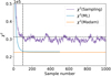 |
Fig. 1. Gibbs chain burn-in as illustrated by the χ2 difference between a given Gibbs sample and the noise-free reference map. The dashed line shows the χ2 level after 100 steps. The χ2 value from Madam is shown by a horizontal line. |
We now pick two sky pixels for closer examination. We arbitrarily select two pixels at a resolution of Nside = 16 from the region excluding strong foregrounds, with pixel indices 200 and 600 in the HEALPix nested pixelization scheme; the locations of these pixels are indicated in Fig. 2, where they are shown on top of the simulated CMB+foreground map.
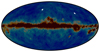 |
Fig. 2. Location of HEALPixNside = 16 pixels 200 and 600 on the sky in nested ordering. The color scale of the underlying map is dimmed to highlight the locations of the two pixels. |
In Fig. 3, we plot the I, Q, U Stokes components of pixel 600 against those of pixel 200. This creates a two-dimensional (2D) plot that illustrates the behaviour of the Gibbs sampling chain. The correct signal value, as taken from the noise-free map, is indicated by a red star. The estimated values necessarily differ from this due to noise. The Madam estimate, representing the maximum-likelihood solution, is shown by an orange star. As expected, the Gibbs sampler in the maximum-likelihood mode approaches the same solution, although we note that the number of steps required to reach it is large.
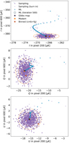 |
Fig. 3. Gibbs chains for the Stokes parameters I, Q and U in pixels 200 and 600 in a HEALPixNside = 16 map with nested ordering. The value in pixel 600 is shown on the y-axis, plotted against the value in pixel 200 (x-axis). Purple dots indicate individual steps during a sampling run, while blue dots indicate steps in a maximum-likelihood run. The orange stars indicate the Madam solution, and orange contours indicate confidence regions based on white noise uncertainties alone. |
In the sampling mode, the map samples fluctuate around the maximum-likelihood solution, revealing the shape of the likelihood distribution. This can be compared to the theoretical white noise distribution. Along with the maximum-likelihood solution for the map, Madam produces a white noise approximation of the noise covariance. This is indicated by orange circles in the same plot. The Gibbs chain tracks the shape of the distribution well, when the burn-in period (shown by gray dots) is discarded. The sampled distribution includes also a contribution from correlated noise, which is missing in the white noise estimate. As the residual is dominated by white noise, however, these are difficult to discern in the pixel plot. In Sect. 4.2 we will further examine the noise residuals in harmonic space, where correlated residuals are visible much more clearly.
The Stokes components (I, Q, U) of the pixelized Gibbs map are shown in the uppermost panel of Fig. 4, adopting a HEALPix resolution of Nside = 512, or 7′ pixel size. All polarization components in this figure have been smoothed with a 1 deg FWHM Gaussian smoothing window to reduce noise.
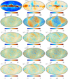 |
Fig. 4. Temperature and polarization maps from simulation. Columns show, from left to right, the Stokes T, Q, and U components. Rows show, from top to bottom, (1) Gibbs map: the mean of maps from the Gibbs chain, as evaluated from 900 samples; (2) absolute residual error as evaluated as the difference between the Gibbs map and the noise-free map; (3) the difference between the Gibbs map and the Madam map derived from the same data set; (4) residual error in Madam for a simulation that does not contain bandpass (i.e., a simulation with same input foreground map for all radiometers) evaluated as the difference between the Madam map and noise-free map; and (5) the difference between the Gibbs map and the maximum-likelihood map. |
The second row of Fig. 4 shows the difference with respect to the noise-free map. This represents residual noise and systematic errors in the Gibbs map. We observe that in addition to white noise, there is also a large-scale signal residual in the polarization component, indicating leakage of temperature signal into polarization. However, when we take the difference between the Gibbs map and the Madam map constructed from the same data, the structure nearly disappears, as shown in the third row. This indicates that the same signal residual is present in the Madam map as well. The leakage is thus not a property of the Gibbs sampling method, but a feature common all mapmaking methods.
As shown below, the source of the leakage is detector-dependent bandpass and beam mismatch, coupled to a frequency-dependent foreground signal. To mitigate this, we have masked the Galactic region during correlated noise estimation. However, the mask size is a trade-off: removing more of the foreground will reduce the leakage, but at the same time this will also remove useful data and make noise reduction more difficult. Here, we are working with the 30 GHz channel, which is particularly cumbersome in this respect, as the foreground signal extends over a large part of the sky.
To pinpoint the origin of the large-scale residual in the second row, we create a simplified simulation data set where the bandpasses of all radiometers are set equal. To do this, we took the bandpass-weighted input sky for radiometer LFI27M and fed it as input to all radiometers, however, with each one always convolving with each radiometer’s own beam. Since running a full Gibbs chain is computationally expensive and knowing that Madam is subject to same leakage, we only ran Madam on the new simulation. The difference between the Madam map and the noise-free reference map is shown in fourth row of Fig. 4. The structure is strongly reduced as compared to the one seen in the second row. This shows that the large-scale structure seen in row 2 is caused by foreground signal residuals in combination with differential instrument responses and associated with bandpass mismatch. This highlights the importance of combined mapmaking and systematics corrections, as discussed by BeyondPlanck Collaboration (2023), and accounting for these types of effects is one of the main motivations for the full BEYONDPLANCK Gibbs sampler.
Finally, in the bottom row of Fig. 4, we show the difference between the Gibbs map (with sampling) and the maximum-likelihood map (last sample from the Gibbs chain with sampling off). The differences between the two are below the 1 μK level.
4.2. Harmonic space
We now proceed to examine the noise residuals in harmonic space, where the correlated residuals are seen more clearly. In Fig. 5 we plot the residual noise spectrum for Madam, maximum-likelihood map, and the Gibbs map. The residual noise spectrum is computed as the angular power spectrum of the difference map between a map estimate and the noise-free map. All three spectra are very close to each other.
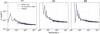 |
Fig. 5. Residual noise spectra for different mapmaking options. The residual noise spectrum is computed as the angular power spectrum of the residual noise map, which, in turn, is obtained as the difference between a map estimate and the noise-free map. |
To show the differences more clearly, we plot ratios of these spectra in Figs. 6 and 7. We use the Madam spectrum as a reference and we plot the ratio of other spectra to it. In Fig. 6 we show the residual noise in the Gibbs map for different numbers of sampling steps. In each case, the map is an average of the Gibbs samples over the indicated number of samples. The burn-in period is excluded in all cases. The spectrum is very close to that of Madam at high multipoles, but differences are seen at the lowest multipoles. In particular, we see that the Gibbs map converges very slowly with number of iterations, resulting in an overall high computational cost. Clearly, a direct solver is highly preferred over the Gibbs approach in applications that only require a single maximum-likelihood solution and no error estimate, as, for instance, is the case in most forward simulation-based analysis pipelines.
We might have hoped for the Gibbs map to yield a lower noise residual, due to the shorter baseline length. However, we did not observe this in our simulations. This is good news for the official Planck analysis, since it indicates that correlated noise at scales below the Madam baseline length (0.25 s) is already negligible. For a few multipoles (ℓ = 4 − 6), Madam yields a lower residual than the Gibbs solver. This can be attributed to numerical differences in the implementation of the noise filter, and is well below the sample variance.
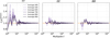 |
Fig. 6. Ratio of the residual noise spectrum of the Gibbs map to that of Madam for different chain lengths. |
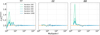 |
Fig. 7. Ratio of the residual noise spectrum of the maximum-likelihood map to that of Madam for different Gibbs chain lengths. |
In a similar manner, Fig. 7 shows the ratio of residual noise spectrum in the maximum-likelihood map to that of the Madam map. Here, the map in question is based on the last sample of a Gibbs chain with the given number of steps and with sampling turned off. We see that more than 500 steps are required for convergence. In Fig. 8 we show in the same plot the residual spectra from Figs. 6 and 7. From both plots, we pick the result with highest number of samples.
 |
Fig. 8. Ratio of residual noise spectrum to that of Madam, for a Gibbs map and for a maximum-likelihood map with the largest available number of samples. The data are the same as in Figs. (6) and (7). |
For the Gibbs sampling approach, the scatter of the samples around the mean estimate provides a direct account of the residual noise and may be used to construct an estimate of the noise bias as follows: we first compute individual noise maps by subtracting the average map from each map sample. We then compute the angular power spectrum of each noise map with the standard anafast tool (Górski et al. 2005) and obtain the noise bias as the mean of these spectra, dividing by N − 1 as usual for a variance estimate.
In Fig. 9 we plot this estimated noise bias together with the average noise spectrum from 101 noise-only Monte Carlo samples, as processed through Madam. The first MC sample is shown in dark grey and represents the same data set as the one used in the validation of the Gibbs sampler. The noise bias and the Monte Carlo average agree very well. We see also that the differences seen in Fig. 8 at low multipoles are small compared with the random scatter between realizations in the noise MC.
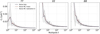 |
Fig. 9. Noise bias from Gibbs chain compared with noise Monte Carlo. Noise MC contains 101 realizations, processed with Madam. The mean of the MC spectra is plotted in brown, and ±1σ regions in light grey. Realization 0 of noise MC is plotted in medium grey. |
We note that unlike the residual noise spectra that require information on the simulation input, the noise bias can be computed from Gibbs chains alone, since it involves only the Gibbs samples and their mean. The procedure is thus available when processing actual measurement data.
4.3. Computational costs
We run the simulation on a 24-core compute node with Intel Xeon E5-2697 (2.7 GHz) processors. On this system, one Madam run on the simulation data set takes 4000 s of wall time (27 core-hours). One Gibbs sampling step with gap filling takes 173 s, while the full cost of a Gibbs chain with 1000 steps is 1150 core-hours (two days in wall-clock time), or more than 40 times the cost of a Madam run. In maximum-likelihood the process is somewhat faster, taking 107 s per iteration, and a total of 360 core-hours for 500 iteration steps; this is still 13 times the cost of Madam. It is thus evident that if one is interested only in the maximum-likelihood solution, the Gibbs procedure is not competitive with more direct methods, such as Madam.
We have also tried running Gibbs sampling without gap filling, which is the most time-consuming step in the procedure, as it requires a conjugate gradient iteration inside every Gibbs step. Since we are dealing here with a full-scale simulation with foreground signal and bandpass effects, the convergence is somewhat slower than what we observed with the pure noise simulation of Sect. 2.3.1. The procedure takes 1814 seconds per Gibbs iteration, and is thus more than ten times slower than the procedure with gap filling, In our test case, the additional memory requirement associated with the gap filling procedure is negligible in comparison with the overall memory requirement.
In Fig. 10, we compare the residual noise as estimated both with gap filling and with the conjugate gradient solution, both in the maximum-likelihood mode. The conjugate gradient option does converge faster, but the differences are in the end negligible.
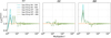 |
Fig. 10. Ratio of residual noise spectrum to that of Madam, with and without gap filling for 199, 299, or 499 samples. |
The most computationally expensive combination is the sampling mode without gap filling. Preliminary tests indicate that this option would take two weeks of wall-clock time, most likely without offering any benefit over the options already studied. Thus, we do not examine this combination further.
5. Conclusions
In this work, we introduce Gibbs sampling as a novel solution to the mapmaking problem for CMB experiments. Gibbs mapmaking can be run in “maximum-likelihood mode” to find the map solution that maximizes the likelihood function, or in “sampling mode” in the case of which the algorithm draws samples from the corresponding posterior distribution. The mean of this distribution gives a best estimate of the underlying true sky, while the scatter of the samples provides an account of the residual noise in the map estimate.
To validate the procedure, we compared the results against those of a direct maximum-likelihood solver (Madam). We demonstrate that with noise sampling disabled, the Gibbs sampling procedure can be used to find the maximum-likelihood map solution. Since the sampler proceeds in small one-dimensional steps through the large multi-dimensional parameter space, the procedure is relatively slow and offers little benefit over direct methods. Even so, this is an important validation step.
The true value of the Gibbs sampling approach lies in error propagation and integration with systematic corrections. In this paper, we demonstrate the first part, namely that Gibbs sampling provides an efficient method to sample the full likelihood distribution surrounding the maximum-likelihood map. In this way, we obtain a reliable estimate of the level of residual noise in the map (noise bias), which is otherwise possible only through Monte Carlo simulations or through the construction of a pixel-to-pixel noise covariance matrix, which is notorious as a computationally demanding task.
We study two ways to deal with gaps in the data: either by solving an exact maximum-likelihood system where flagged samples are assigned an infinite variance or by including the gaps in the Gibbs process as another variable to sample. The latter translates into filling the gaps with a new white noise realization at every step. In our test case, gap filling turns out to be significantly more efficient and, thus, we set this as our method of choice. It is worth bearing in mind, however, that gap filling comes with an increased memory requirement, which may become prohibitive in other user cases.
The full power of Gibbs sampling as a mapmaking solution is realized in cases where mapmaking and noise removal are included as a part of a full Gibbs sampling machinery, including foreground modeling and estimation of instrument effects. This is the goal of the larger BEYONDPLANCK project.
Acknowledgments
We thank Prof. Pedro Ferreira and Dr. Charles Lawrence for useful suggestions, comments and discussions. We also thank the entire Planck and WMAP teams for invaluable support and discussions, and for their dedicated efforts through several decades without which this work would not be possible. The current work has received funding from the European Union’s Horizon 2020 research and innovation programme under grant agreement numbers 776282 (COMPET-4; BEYONDPLANCK), 772253 (ERC; BITS2COSMOLOGY), and 819478 (ERC; COSMOGLOBE). In addition, the collaboration acknowledges support from ESA; ASI and INAF (Italy); NASA and DoE (USA); Tekes, Academy of Finland (grant no. 295113), CSC, and Magnus Ehrnrooth foundation (Finland); RCN (Norway; grant nos. 263011, 274990); and PRACE (EU).
References
- Ashdown, M. A. J., Baccigalupi, C., Balbi, A., et al. 2007a, A&A, 471, 361 [NASA ADS] [CrossRef] [EDP Sciences] [Google Scholar]
- Ashdown, M. A. J., Baccigalupi, C., Balbi, A., et al. 2007b, A&A, 467, 761 [NASA ADS] [CrossRef] [EDP Sciences] [Google Scholar]
- Ashdown, M. A. J., Baccigalupi, C., Bartlett, J. G., et al. 2009, A&A, 493, 753 [NASA ADS] [CrossRef] [EDP Sciences] [Google Scholar]
- Bersanelli, M., Mandolesi, N., Butler, R. C., et al. 2010, A&A, 520, A4 [NASA ADS] [CrossRef] [EDP Sciences] [Google Scholar]
- BeyondPlanck Collaboration (Andersen, K. J., et al.) 2023, A&A, 675, A1 (BeyondPlanck SI) [Google Scholar]
- Burigana, C., Malaspina, M., Mandolesi, N., et al. 1999, ArXiv e-prints [arXiv:astro-ph/9906360] [Google Scholar]
- Delabrouille, J. 1998, A&AS, 127, 555 [NASA ADS] [CrossRef] [EDP Sciences] [Google Scholar]
- Eriksen, H. K., Jewell, J. B., Dickinson, C., et al. 2008, ApJ, 676, 10 [Google Scholar]
- Galloway, M., Andersen, K. J., Aurlien, R., et al. 2023, A&A, 675, A3 (BeyondPlanck SI) [NASA ADS] [CrossRef] [EDP Sciences] [Google Scholar]
- Górski, K. M., Hivon, E., Banday, A. J., et al. 2005, ApJ, 622, 759 [Google Scholar]
- Ihle, H. T., Bersanelli, M., Franceschet, C., et al. 2023, A&A, 675, A6 (BeyondPlanck SI) [NASA ADS] [CrossRef] [EDP Sciences] [Google Scholar]
- Keihänen, E., & Reinecke, M. 2012, A&A, 548, A110 [NASA ADS] [CrossRef] [EDP Sciences] [Google Scholar]
- Keihänen, E., Kurki-Suonio, H., Poutanen, T., Maino, D., & Burigana, C. 2004, A&A, 428, 287 [NASA ADS] [CrossRef] [EDP Sciences] [Google Scholar]
- Keihänen, E., Kurki-Suonio, H., & Poutanen, T. 2005, MNRAS, 360, 390 [NASA ADS] [CrossRef] [Google Scholar]
- Keihänen, E., Keskitalo, R., Kurki-Suonio, H., Poutanen, T., & Sirviö, A. 2010, A&A, 510, A57 [CrossRef] [EDP Sciences] [Google Scholar]
- Kurki-Suonio, H., Keihänen, E., Keskitalo, R., et al. 2009, A&A, 506, 1511 [NASA ADS] [CrossRef] [EDP Sciences] [Google Scholar]
- Maino, D., Burigana, C., Maltoni, M., et al. 1999, A&AS, 140, 383 [NASA ADS] [CrossRef] [EDP Sciences] [Google Scholar]
- Maino, D., Burigana, C., Górski, K. M., Mandolesi, N., & Bersanelli, M. 2002, A&A, 387, 356 [NASA ADS] [CrossRef] [EDP Sciences] [Google Scholar]
- Planck Collaboration II. 2014, A&A, 571, A2 [NASA ADS] [CrossRef] [EDP Sciences] [Google Scholar]
- Planck Collaboration II. 2016, A&A, 594, A2 [NASA ADS] [CrossRef] [EDP Sciences] [Google Scholar]
- Planck Collaboration IV. 2016, A&A, 594, A4 [NASA ADS] [CrossRef] [EDP Sciences] [Google Scholar]
- Planck Collaboration IV. 2020, A&A, 641, A4 [NASA ADS] [CrossRef] [EDP Sciences] [Google Scholar]
- Planck Collaboration V. 2020, A&A, 641, A5 [NASA ADS] [CrossRef] [EDP Sciences] [Google Scholar]
- Poutanen, T., de Gasperis, G., Hivon, E., et al. 2006, A&A, 449, 1311 [NASA ADS] [CrossRef] [EDP Sciences] [Google Scholar]
- Prézeau, G., & Reinecke, M. 2010, ApJS, 190, 267 [CrossRef] [Google Scholar]
- Reinecke, M., Dolag, K., Hell, R., Bartelmann, M., & Enßlin, T. A. 2006, A&A, 445, 373 [NASA ADS] [CrossRef] [EDP Sciences] [Google Scholar]
- Sutton, D., Johnson, B. R., Brown, M. L., et al. 2009, MNRAS, 393, 894 [NASA ADS] [CrossRef] [Google Scholar]
- Svalheim, T. L., Zonca, A., Andersen, K. J., et al. 2023, A&A, 675, A9 (BeyondPlanck SI) [NASA ADS] [CrossRef] [EDP Sciences] [Google Scholar]
- Wehus, I. K., Næss, S. K., & Eriksen, H. K. 2012, ApJS, 199, 15 [NASA ADS] [CrossRef] [Google Scholar]
All Figures
|
Fig. 1. Gibbs chain burn-in as illustrated by the χ2 difference between a given Gibbs sample and the noise-free reference map. The dashed line shows the χ2 level after 100 steps. The χ2 value from Madam is shown by a horizontal line. |
| In the text | |
|
Fig. 2. Location of HEALPixNside = 16 pixels 200 and 600 on the sky in nested ordering. The color scale of the underlying map is dimmed to highlight the locations of the two pixels. |
| In the text | |
|
Fig. 3. Gibbs chains for the Stokes parameters I, Q and U in pixels 200 and 600 in a HEALPixNside = 16 map with nested ordering. The value in pixel 600 is shown on the y-axis, plotted against the value in pixel 200 (x-axis). Purple dots indicate individual steps during a sampling run, while blue dots indicate steps in a maximum-likelihood run. The orange stars indicate the Madam solution, and orange contours indicate confidence regions based on white noise uncertainties alone. |
| In the text | |
|
Fig. 4. Temperature and polarization maps from simulation. Columns show, from left to right, the Stokes T, Q, and U components. Rows show, from top to bottom, (1) Gibbs map: the mean of maps from the Gibbs chain, as evaluated from 900 samples; (2) absolute residual error as evaluated as the difference between the Gibbs map and the noise-free map; (3) the difference between the Gibbs map and the Madam map derived from the same data set; (4) residual error in Madam for a simulation that does not contain bandpass (i.e., a simulation with same input foreground map for all radiometers) evaluated as the difference between the Madam map and noise-free map; and (5) the difference between the Gibbs map and the maximum-likelihood map. |
| In the text | |
|
Fig. 5. Residual noise spectra for different mapmaking options. The residual noise spectrum is computed as the angular power spectrum of the residual noise map, which, in turn, is obtained as the difference between a map estimate and the noise-free map. |
| In the text | |
|
Fig. 6. Ratio of the residual noise spectrum of the Gibbs map to that of Madam for different chain lengths. |
| In the text | |
|
Fig. 7. Ratio of the residual noise spectrum of the maximum-likelihood map to that of Madam for different Gibbs chain lengths. |
| In the text | |
|
Fig. 8. Ratio of residual noise spectrum to that of Madam, for a Gibbs map and for a maximum-likelihood map with the largest available number of samples. The data are the same as in Figs. (6) and (7). |
| In the text | |
|
Fig. 9. Noise bias from Gibbs chain compared with noise Monte Carlo. Noise MC contains 101 realizations, processed with Madam. The mean of the MC spectra is plotted in brown, and ±1σ regions in light grey. Realization 0 of noise MC is plotted in medium grey. |
| In the text | |
|
Fig. 10. Ratio of residual noise spectrum to that of Madam, with and without gap filling for 199, 299, or 499 samples. |
| In the text | |
Current usage metrics show cumulative count of Article Views (full-text article views including HTML views, PDF and ePub downloads, according to the available data) and Abstracts Views on Vision4Press platform.
Data correspond to usage on the plateform after 2015. The current usage metrics is available 48-96 hours after online publication and is updated daily on week days.
Initial download of the metrics may take a while.