| Issue |
A&A
Volume 674, June 2023
Gaia Data Release 3
|
|
|---|---|---|
| Article Number | A2 | |
| Number of page(s) | 28 | |
| Section | Catalogs and data | |
| DOI | https://doi.org/10.1051/0004-6361/202243680 | |
| Published online | 16 June 2023 | |
Gaia Data Release 3
Processing and validation of BP/RP low-resolution spectral data
1
Institute of Astronomy, University of Cambridge, Madingley Road, Cambridge, CB3 0HA, UK
2
Institut de Ciències del Cosmos (ICC), Universitat de Barcelona (IEEC-UB), c/ Martí i Franquès, 1, 08028 Barcelona, Spain
3
INAF – Osservatorio di Astrofisica e Scienza dello Spazio di Bologna, Via Gobetti 93/3, 40129 Bologna, Italy
4
Max Planck Institute for Astronomy, Königstuhl 17, 69117 Heidelberg, Germany
5
Institute for Astronomy, School of Physics and Astronomy, University of Edinburgh, Royal Observatory, Blackford Hill, Edinburgh, EH9 3HJ, UK
6
Kavli Institute for Cosmology, Institute of Astronomy, Madingley Road, Cambridge, CB3 0HA, UK
7
INAF – Osservatorio Astrofisico di Arcetri, Largo E. Fermi, 5, 50125 Firenze, Italy
8
INAF – Osservatorio Astronomico di Roma, via Frascati 33, 00078 Monte Porzio Catone (Roma), Italy
9
Space Science Data Center – ASI, Via del Politecnico SNC, 00133 Roma, Italy
10
School of Physics & Astronomy, University of Leicester, Leicester, LE9 1UP, UK
11
Leiden Observatory, Leiden University, Niels Bohrweg 2, 2333 CA Leiden, The Netherlands
12
Institut d’Astrophysique et de Géophysique, Université de Liège, 19c, Allée du 6 Août, 4000 Liège, Belgium
13
INAF – Osservatorio Astronomico d’Abruzzo, Via Mentore Maggini, 64100 Teramo, Italy
14
Royal Observatory of Belgium, Ringlaan 3, 1180 Brussels, Belgium
15
IAC – Instituto de Astrofisica de Canarias, Via Láctea s/n, 38200 La Laguna S.C., Tenerife, Spain
16
SRON Netherlands Institute for Space Research, Niels Bohrweg 4, 2333 CA Leiden, The Netherlands
17
Ruder Bošković Institute, Bijenička cesta 54, Zagreb, Croatia
18
INAF – Osservatorio Astronomico di Brera, Via E. Bianchi, 46, 23807 Merate (LC), Italy
19
STFC, Rutherford Appleton Laboratory, Harwell, Didcot, OX11 0QX, UK
20
Dpto. de Inteligencia Artificial, UNED, c/ Juan del Rosal 16, 28040 Madrid, Spain
21
INAF – Osservatorio Astronomico di Padova, Vicolo Osservatorio 5, 35122 Padova, Italy
Received:
30
March
2022
Accepted:
29
June
2022
Abstract
Context. Blue (BP) and Red (RP) Photometer low-resolution spectral data are one of the exciting new products in Gaia Data Release 3 (Gaia DR3). These data have also been used to derive astrometry and integrated photometry in Gaia Early Data Release 3 and astrophysical parameters and Solar System object reflectance spectra in Gaia DR3.
Aims. In this paper, we give an overview of the processing techniques that allow raw satellite data of multiple transits per source to be converted into combined spectra calibrated to an internal reference system, resulting in low-resolution BP and RP mean spectra. We describe how we overcome challenges due to the complexity of the on-board instruments and to the various observation strategies. Furthermore, we show highlights from our scientific validation of the results. This work covers the internal calibration of BP/RP spectra to a self-consistent mean instrument, while the calibration of the BP/RP spectra to the absolute reference system of physical flux and wavelength is covered by one of the accompanying Gaia DR3 papers.
Methods. We calibrate about 65 billion individual transit spectra onto the same mean BP/RP instrument through a series of calibration steps, including background subtraction, calibration of the CCD geometry, and an iterative procedure for the calibration of CCD efficiency as well as variations of the line-spread function and dispersion across the focal plane and in time. The calibrated transit spectra are then combined for each source in terms of an expansion into continuous basis functions. We discuss the configuration of these basis functions.
Results. Time-averaged mean spectra covering the optical to near-infrared wavelength range [330, 1050] nm are published for approximately 220 million objects. Most of these are brighter than G = 17.65 but some BP/RP spectra are published for sources down to G = 21.43. Their signal-to-noise ratio (S/N) varies significantly over the wavelength range covered, and with magnitude and colour of the observed objects, with sources around G = 15 having a S/N above 100 in some wavelength ranges. The top-quality BP/RP spectra are achieved for sources with magnitudes 9 < G < 12, with S/N reaching 1000 in the central part of the RP wavelength range. Scientific validation suggests that the internal calibration was generally successful. However, there is some evidence for imperfect calibrations at the bright end G < 11, where calibrated BP/RP spectra can exhibit systematic flux variations that exceed their estimated flux uncertainties. We also report that, due to long-range noise correlations, BP/RP spectra can exhibit wiggles when sampled in pseudo-wavelength.
Conclusions. The Gaia DR3 data products are the expansion coefficients and corresponding covariance matrices for BP and RP separately. Users are encouraged to work with the data in this format, with full covariance information showing that correlations between coefficients are typically very low. Documentation and instructions on how to access and use BP/RP spectral data from the archive are also provided.
Key words: instrumentation: photometers / instrumentation: spectrographs / catalogs / surveys / techniques: photometric / techniques: spectroscopic
Corresponding author: F. De Angeli, e-mail: This email address is being protected from spambots. You need JavaScript enabled to view it. .
© The Authors 2023
 Open Access article, published by EDP Sciences, under the terms of the Creative Commons Attribution License (https://creativecommons.org/licenses/by/4.0), which permits unrestricted use, distribution, and reproduction in any medium, provided the original work is properly cited.
This article is published in open access under the Subscribe to Open model. This email address is being protected from spambots. You need JavaScript enabled to view it. to support open access publication.
1. Introduction
The European Space Agency (ESA) mission Gaia (Gaia Collaboration 2016) has already released three catalogues to the astronomical community; of increasing richness in terms of content, precision, and accuracy. Researchers from many branches of astrophysics have shown great interest in the published data, leading to the publication of more than 6000 refereed papers based on Gaia data to date1.
With respect to the previous Gaia Early Data Release 3, Gaia Data Release 3 (Gaia DR3; Gaia Collaboration 2023b) introduces a number of new data products based on the same source catalogue, including a total of 1.8 billion objects and based on a period of 34 months of satellite operations. A large fraction of the objects in the catalogue has astrophysical parameters determined from the medium (Radial Velocity Spectrometer, RVS) and low-resolution (Blue and Red Photometers, BP and RP) spectral data as well as from the photometric data (Andrae et al. 2023; Creevey et al. 2023). For many of these objects, the actual RVS and/or BP/RP data themselves are part of the release; RVS spectra are released for about 1 million sources, while mean low-resolution BP/RP spectra are available for about 220 million objects, which were selected to have a reasonable number of observations and to be sufficiently bright to ensure good signal-to-noise ratio (S/N) at this stage in the mission. New estimates of mean radial velocities, variable-star classification, and epoch photometry are released for a subset of sources. A large set of Solar System objects, including new discoveries, with preliminary orbital solutions and individual epoch observations are available in the Gaia DR3 release. A selection of these also have their reflectance spectra estimated from the epoch BP/RP spectral data (Gaia Collaboration 2023a). The release also includes results for non-single stars, quasars, and extended objects. Finally, an additional data set is also released, called the Gaia Andromeda Photometric Survey (GAPS), which consists of the photometric time series for all sources located in a 5.5 degree radius field centred on the Andromeda galaxy (Evans et al. 2023). A number of papers have been prepared by the Data Processing and Analysis Consortium (DPAC) describing all aspects of the data processing and the results of the performance verification activities. In this paragraph, we have only included specific citations to papers that have made use of the BP/RP spectral data. A full list is available at2.
This paper focuses on the BP/RP low-resolution spectral data and on the processing that led to the generation of the BP/RP spectra included in Gaia DR3. Some aspects of the BP/RP processing have already been introduced in recent papers which should be considered essential companions to this one. In particular, calibrations that were also required for the generation of the BP/RP integrated photometry are detailed in Riello et al. (2021) and are described only very briefly in this paper. The algorithm adopted for the internal calibration of the BP/RP spectral data is presented in the dedicated paper Carrasco et al. (2021). We refer to Carrasco et al. (2021) for a detailed justification of the model definition and complement that work by providing information on the actual model configuration adopted to generate the Gaia DR3 BP/RP spectra. The focus of this paper is the processing leading to the generation of a homogeneous catalogue of source spectra from the raw Gaia BP/RP observations. While Gaia DR3 does not provide access to individual observations, knowing the complexities related to the instruments, observing strategies, and processing is important to understand the final product. This paper also contains useful information about the representation of the spectra and the strategies adopted to optimise it and minimise the noise in the final spectra. The validation shown in this paper focuses on these aspects. The calibration of the BP/RP spectral data to the absolute reference system (both in terms of flux and wavelength) is detailed in Montegriffo et al. (2023). This latter should be seen as an essential companion to this paper. Users interested in systematic effects present in the final BP/RP products should refer to that paper, which presents the results of the validation of the externally calibrated data with respect to external absolute spectra. Finally, Babusiaux et al. (2023) present the overall results of the independent DPAC validation process, with useful insights into the limitations and recommendations for BP/RP spectral data.
The paper outline is the following: in Sect. 2 we describe the general concept of low-resolution spectroscopic data and the specific aspects of the Gaia BP/RP data that are relevant for this paper; Sect. 3 is dedicated to the data processing, with considerations as to the processing strategies, algorithms, and results; a description of the composition of the BP/RP spectral catalogue in Gaia DR3 is provided in Sect. 4; highlights from the internal validation activities are given in Sects. 5 and 6 offer some recommendations for the users.
2. Input data
During its operations, the Gaia satellite scans the entire sky every 6 months while spinning around its principal axis and precessing around the Earth-Sun direction. The light from two fields of view (FoVs) is focused on the same focal plane. Images of sources crossing the focal plane move over an array of charge-coupled devices (CCDs) operating in time-delayed integration (TDI) mode, such that the charges generated by a point-like astronomical source are clocked through the CCD at the same speed as the apparent motion of the source caused by the satellite scanning motion. In the following, we use transit to refer to a full focal plane crossing of a source and CCD transit when referring to the crossing of a single CCD, generating one observation.
Throughout this paper, time is expressed in on-board mission time (OBMT) in units of satellite revolutions (1 OBMT-Rev =21 600 s). A formula to convert OBMT to barycentric coordinate time is provided by Eq. (3) in Gaia Collaboration (2016). In the focal plane array (see Fig. 4 in Gaia Collaboration 2016, or Fig. 2 in Carrasco et al. 2021), the CCDs are arranged in rows (in the along-scan direction, AL) and strips (in the across-scan direction, AC). The largest section of the focal plane array (including 62 astrometric field (AF) CCDs, arranged in seven rows of nine CCDs each, except for one row where there are only eight) is dedicated to the collection of the observations in the broad G-band which are used for astrometric measurements and photometry. Following these, two strips of seven CCDs each are dedicated to the BP and RP instruments. Finally, four rows and three strips of CCDs collect the RVS observations. Not all sources crossing the focal plane will also cross the RVS CCDs.
Colour information for all sources is essential to achieving the high accuracy that characterises the Gaia astrometry. An initial design – where the flux of sources in a variety of medium bands would be measured on different CCD strips to fulfil this requirement (Jordi et al. 2006) – was abandoned in favour of low-resolution aperture prism spectroscopy. This observational technique is frequently used to obtain a large number of spectra with a single exposure in large-scale astronomic surveys, starting from the Draper catalogue in the early 20th century (Pickering 1890) all the way to future applications such as in Euclid (Costille et al. 2016) and NGRST (formerly known as WFIRST Akeson et al. 2019). The BP/RP instruments were added to the satellite payload to collect this data covering the wavelength ranges [330, 680] nm and [640, 1050] nm, respectively, with varying resolution depending on the position in the spectrum and on the CCD (the resolution covers the range 100 to 30 for BP and 100 to 70 for RP in λ/Δλ; see Fig. 3 in Carrasco et al. 2021).
In normal operation mode, observations transmitted to the ground from the satellite are cut-outs of a small area surrounding the position where each source was detected on board. In the case of BP/RP observations, because of the need to cover the full range of the dispersed light, these cut-outs (windows in Gaia terminology) need to be much longer in the direction in which the light is dispersed, which is aligned with the AL direction. This is why the size of the BP/RP windows is 60 pixels in AL (as opposed to a maximum of 18 pixels for the AF windows assigned to the brightest objects) by 12 pixels in AC direction, corresponding to an area in the sky of approximately 3.5 by 2.1 arcsec3. This affects the possibility to assign different windows to nearby sources in crowded regions. As a consequence, not all detections result in a BP/RP observation and the average number of BP/RP observations is lower than the average number of transits per source on the focal plane. Partly overlapping windows can in some cases be allocated by the on-board software. When this happens, the window of the brightest sources is transmitted fully to the ground, while only the non-overlapping section of the other window is transmitted to the ground. These truncated windows are not included in the data leading to Gaia DR3 as they are normally rather disturbed by the nearby brighter source and require special treatment which will only be implemented for future data releases.
Observations on board can be taken in different configurations depending on the on-board magnitude estimate of the source. The activation of a given configuration can also affect simultaneous observations nearby.
Different configuration aspects include the AC resolution within a window which is only achieved for sources brighter than 11.5 mag in the G-band, while windows assigned to fainter sources are binned in the AC direction on board before transmission, resulting in a spectrum with 60 AL samples, where each sample contains the overall flux measurement from 12 pixels. Figure 1 shows the case of a 2D spectrum. The top panel shows the 1D spectrum resulting from the binning in the AC direction. The shape of the 1D spectrum is defined by the combined effect of the response curve, the line spread function (LSF), and the dispersion. The flux from a point-like source is dispersed in the AL direction. The flux at each wavelength is further spread according to the LSF at that wavelength. As a result, each sample in the spectrum, in addition to the local photons, will contain alien photons with different wavelengths. The instrument response, including the filter transmission curve, modulates the flux, only allowing light from a given wavelength range to be detected. A well-centred point-like source should have no flux close to the edge of the observed window. The purpose of the different window strategy for sources fainter than 11.5 mag is to limit the volume of the data that needs downloading from the satellite and to reduce the readout noise. In the following, we refer to these as different window classes (WCs) and in particular to 2D (where the AC resolution is preserved) versus 1D (where binning AC occurs) spectra, respectively. It should be noted that all BP/RP spectra available in Gaia DR3 are 1D (i.e. flux values corresponding to positions in the AL coordinate or wavelength when the external calibration is applied). Spectra acquired with a 2D configuration on board are flattened to 1D during the calibration process: a simple sum of the samples in the same AC column is adopted for consistency with the on-board AC binning algorithm.
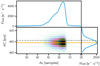 |
Fig. 1. Example of a 2D BP spectrum. The central panel shows the observed spectrum. The dashed and continuous horizontal lines show the AC centre of the window and the AC predicted position based on the source astrometry, the satellite attitude, and the BP CCD geometry. The top and right panels show the result of binning in the AC and AL directions, respectively. The AL coordinate is given in units of samples. |
An ad hoc strategy is also available to prevent saturation when observing bright sources. Different gates can be activated at different locations in the CCD to limit the section of the CCD where the charges are accumulated and therefore effectively reduce the exposure time. The exposure time of an ungated observation is approximately 4.4 s, and the shortest gate active in BP/RP (Gate05) reduces this to 0.06 s. Each gate is activated on board as required based on a configured set of magnitude ranges and the on-board magnitude estimated for each transit. The configuration changes for different instruments (BP/RP) and across the focal plane (even within a CCD); see Fig. 2 for the distribution of different gate and WC configuration versus on-board magnitude for BP and RP. As already mentioned, the selection of the appropriate gate configuration is based on the on-board magnitude estimate which can show up to 0.5 mag uncertainties at the bright end. This implies that a given source may be observed in different gate configurations in different transits. Some of these gate configurations will be suboptimal and therefore some saturation cannot be excluded. Moreover the activation of a gate will affect all observations taken at the same time (within 60 pixels or 0.06 s AL) in the same CCD, thus generating gated observations for faint sources that would normally be observed without any gate. This can also cause what are called complex gate cases, where different gates are active in different sections of a window. Complex gate cases are also not included in the processing leading to Gaia DR3.
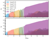 |
Fig. 2. Distribution of the number of BP/RP observations acquired in BP (top panel) and RP (bottom panel) with a given gate and WC configuration vs. on-board magnitude labelled as GVPU. The gated observations for sources fainter than ≈11.5 mag in the G-band are due to occasional alignment of these sources with brighter objects triggering the activation of a gate. |
Figure 3 shows the implications for the fraction of BP (top) and RP (bottom) transits available for processing of some of the mission aspects mentioned in this section (size of BP/RP windows, gates, and truncation). The different curves show the fraction of transits that will not contribute a BP/RP observation to the processing leading to the Gaia DR3 catalogue for various reasons: the blue curve shows the fraction of BP transits affected by truncation, the red line those acquired with a complex gate, the orange line shows the fraction of transits that do not have a BP or RP window acquired, and the green line simply shows the sum of the three previous quantities and therefore the fraction of transits that will not have an observation that can be processed at this stage. Both fractions of truncated and not-acquired windows increase significantly at the faint end, as expected.
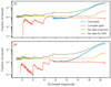 |
Fig. 3. Fraction of transits that will not contribute a BP/RP observation to the processing leading to Gaia DR3 due to either the window not having been acquired (orange line), or to the window being truncated (blue line), or to the window having been observed with multiple gates active within the window (red line). The green line shows the total effect. This is shown as a function of the on-board magnitude estimate as this is the parameter that defines the observation strategy applied to each observation. Truncation for instance is only applied to 1D windows and therefore the corresponding fraction is zero for on-board magnitude brighter than 11.5 mag. |
The total number of transits acquired in the period covered by Gaia DR3 was almost 78 billion. The processing of the BP/RP spectral data produced calibrated BP/RP epoch spectra (i.e. spectra generated from one single observation) for about 65 billion transits, and mean BP/RP spectra (i.e. spectra averaged over the many observations for a given source) for more than 2 billion sources. Not all transits or sources had a complete set of BP and RP spectra. Section 4 provides more information on the selection criteria that lead to the composition of the Gaia DR3 catalogue containing BP/RP spectra for about 220 million sources.
3. Processing
When calibrating the BP/RP data, the characteristics of the various CCDs, the effects introduced by the different optical paths for the two FoVs and by the configuration activated for each observation, and the variation in time of all these elements need to be taken into account. We refer to a set of validity time range (i.e. the interval in time where a given calibration is applicable), CCD, FoV, WC, and gate as a configuration or calibration unit. A set of calibrations per calibration unit (for a total of several tens of thousands of configurations) is produced as part of the instrument calibration process to describe each effect that needs calibrating. Due to the complexity of the system (effectively equivalent to many instruments), the calibration of the data cannot rely on any existing catalogue of standards (all too limited in number and quality), but needs to be solved for internally in the first instance using a large subset of the BP/RP data themselves. This subset is selected to contain data for a sufficiently large catalogue of sources (referred to as calibrators; see Sect. 3.2) covering all calibration units as homogeneously as possible within the limits imposed by nature (e.g., in terms of magnitude and colour distribution). The goal of the internal calibration is to define a reference instrument which is homogeneous across all configurations and time. It is then the responsibility of the external or absolute calibration to define the link between the internal system and the absolute system using a carefully assembled catalogue of spectro-photometric calibrators (Pancino et al. 2021; Marinoni et al. 2016; Altavilla et al. 2015, 2021) and other objects that present features in their spectra that are useful to calibrate specific aspects of the instrument and for which suitable absolute spectra are already available. The internal reference system is defined by the calibrations, that is, the actual calibration coefficients. Once the reference system is established, all the data can be brought to the same system by applying the calibrations. The same approach has been followed for the processing of the Gaia photometric data (Carrasco et al. 2016). In this paper, we focus on the internal calibration of the BP/RP spectral data, while the external calibration is the subject of Montegriffo et al. (2023).
The internal calibration includes many different individual calibration steps that are solved for in separate stages of the data processing, often relying on different subsets of calibrators and requiring different strategies for accessing the data in an optimal way. Figure 4 shows a schematic overview of the major steps and dependencies of the process starting from the input raw observed spectra until the output mean spectra.
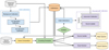 |
Fig. 4. Schematic view of the processing leading to the generation of the BP/RP mean spectra in Gaia DR3. |
The two main inputs to the process are the BP/RP observed spectra and the source catalogue containing astrometry and photometry information for all sources observed so far. In the flow diagram, dashed lines are used to represent data flow for calibrators only, while solid lines are used to indicate that the entire set of the observed spectra is used as input into a given stage. The process flows from left to right and top to bottom. The first calibrations are those grouped in the Initial Calibrations block (see Sect. 3.1), which are repeated after the crowding assessment to ensure only the best-suited data are used. The output of these calibrations is part of a database of calibrations that are needed in various stages of the process. The other block of calibrations is the one labelled Flux and LSF Calibration (see Sect. 3.3), which can only start after the initial calibrations are finalised. This is an iterative process that calibrates the effects of differences in response, varying LSF across the focal plane, and small deviations from the nominal differential dispersion functions. When all calibrations are defined, the final steps in the process produce the output catalogues of internally calibrated spectra. In this paper we focus on the mean source spectra (see Sect. 3.4), which are produced using all the observations for a given source, while the process producing the epoch spectra (one calibrated spectrum per observed spectrum) is only briefly described in Sect. 3.3.1. While the epoch spectra are not directly available in Gaia DR3, they contributed to the generation of mean reflectances for Solar System objects.
3.1. Initial calibrations
Starting at the top left corner from the raw BP/RP data, we find a first block of calibrations labelled Initial Calibrations. Some of these have been described in previous papers (Riello et al. 2018, 2021) because they are also required for the photometric processing: the computation of integrated BP/RP fluxes and spectrum shape coefficients (SSCs) – which are the input to the photometric processing together with the corresponding G-band fluxes – requires the application of the background and AL geometric calibrations.
The background calibration for Gaia DR3 is a two-stage process: high-resolution stray-light maps are first generated to remove effects due to diffraction from loose fibres in the sun shield (Fabricius et al. 2016); a k-nearest neighbour approach is then applied to the map residuals to describe the local astrophysical background (e.g., non-resolved sources, diffuse light from nearby objects, zodiacal light) at a resolution of about 25 arcsec. More details about this calibration and a validation of the results are provided in Riello et al. (2021) (see their Sect. 3.2).
Due to small inaccuracies in on-board detection and window assignment, sources are usually not perfectly centred within the acquired windows. In order to be able to align spectra taken at different times and in different configurations for a given source, we need to rely on a detailed geometric calibration, an accurate attitude reconstruction, and high-accuracy astrometry for all observed sources. Attitude and astrometry are inputs to the BP/RP processing, while the geometric calibration is a product of one of the calibration steps (AL and AC Geometric Calibration in Fig. 4). The AL geometric calibration provides a correction in the AL direction to the location of a reference wavelength within the observed window as computed using our pre-launch knowledge of the CCD geometry. Once the reference wavelength is located within the window, this can also be used as reference position for the application of nominal differential dispersion functions that mitigates the difference in dispersion across the focal plane. More details about the AL geometric calibration can be found in Riello et al. (2018) and Carrasco et al. (2016). The AC geometric calibration is similarly defined as a correction to the predicted location on the source centroid in the AC direction as obtained from pre-launch knowledge of the CCD geometry, the satellite attitude, and the source astrometry.
The two geometric calibrations (AL and AC) are required for the generation of accurate BP/RP transit time and AC coordinate predictions for all sources in the catalogue, that is, the Scene Computation in Fig. 4. An assessment of the crowding status of a given transit (the assessment needs to be done per transit rather than per source because of the overlap of the two FoVs on the focal plane and the varying scan direction) cannot be purely based on the acquired surrounding windows. As we have already mentioned, crowding and priorities imply that a given source may not be assigned a window in the BP/RP CCDs, and therefore such an assessment would be incomplete. This is why the scene is generated starting from the source catalogue containing objects that have been observed at all times during the mission operations so far. The astrometric information from the source catalogue is combined with the satellite attitude and with the geometric calibrations of the CCD of interest to generate the predictions. A detailed description of the scene computation and crowding evaluation has been included in Riello et al. (2021) because of its relevance in the generation of crowding information included in Gaia EDR3.
As shown in the schematic view, the Initial Calibrations are repeated after the Crowding Evaluation to include only data that have been assessed as not significantly affected by crowding, thus minimising the disturbing effects of crowding on the calibrations. After this second run of the Initial Calibrations, the spectra are used to generate integrated BP/RP fluxes and Spectrum Shape Coefficients (a set of ad hoc filters designed for the photometric calibration; see Riello et al. 2021). At this point, 2D spectra are marginalised in the AC direction to form 1D spectra and all subsequent processing only deals with 1D spectra.
3.2. Internal calibrators
Each calibration step normally relies on a specifically designed set of calibration data. For the background calibration, for instance, only Virtual Objects (empty windows acquired on a predefined pattern for calibration purposes) and observations of objects fainter than G = 18.95 mag were used to avoid systematic effects due to the target source flux biasing the background measurement obtained from the first and last few samples in the window. For the AL geometric calibration, the need to find the best alignment of the spectra implies a requirement that their shape be similar and therefore that the colour range of calibrators be quite narrow. Finally, for the AC geometric calibration, 2D spectra are essential in order to resolve the location of the peak in the flux distribution in the AC direction.
In the case of the Flux and LSF calibration, the most important requirement is that all configurations are well covered by the set of calibrators. Calibrators covering more than one configuration are particularly valuable. This is naturally the case for time, FoV, and CCD (sources are observed an average of about 40 times in the time range covered by Gaia DR3, in different FoVs and CCDs), while in the case of gates and WC, only a limited subset of the calibrators will have observations in two or more observation configurations; these will be sources that have a magnitude close to the boundary of the magnitude range where that strategy is active and that, due to inaccuracies of the on-board magnitude estimate, may therefore be observed in different configurations in subsequent transits. The following criteria were tailored to ensure a clean but well-populated set of calibrators. Only sources in the colour range −2.0 < (GBP − GRP)< 5.0 mag and magnitude range 5.0 < G < 17.0 mag based on the Gaia DR2 photometry were considered. Sources with G-band magnitude brighter than 11.5 mag were selected as long as they had more than ten transits in BP/RP, which is to ensure that the magnitude range where gates are activated is well covered. Sources fainter than 11.5 mag with at least one 2D or gated observation were selected as long as their number of usable transits was larger than the median of the distribution of the number of transits in the same HEALPix pixel of level 6 minus the uncertainty estimated as the median absolute deviation of the distribution. This particular criterion was designed to avoid cases of faint sources that happened to be observed in a gated configuration because of their proximity to a bright object: in these cases, a large fraction of the transits of the faint source would be acquired with multiple gates (a case that is not currently processed) and would therefore not be usable. Only the few transits acquired when the two sources were observed at the same time would be usable. These would be likely to be significantly disturbed by the nearby bright source and therefore hardly suitable for calibration purposes. Finally, to enhance the fraction of sources with extreme colours (within the allowed range) with respect to sources of intermediate colours, the distribution of sources fainter than 11.5 mag that are only observed in ungated configuration and in 1D window strategy is flattened in colour as much as possible. Blue sources in particular are essential to constrain the internal calibration at short wavelengths and a poor calibration for blue sources may affect the absolute calibration given that the catalogue of external calibrators contains a large fraction of white dwarfs. The colour flattening is achieved in ranges of magnitude and HEALPix pixels by considering the distribution in colour of the possible calibrators and selecting calibrators from the least populated colour ranges first: each time a number of calibrators are added to the list of selected calibrators from the least populated colour bin, an equal number of calibrators are selected from each of the other colour ranges, giving priority to the sources with the largest number of transits. The process is repeated until the number of selected calibrators has reached the desired number of calibrators per HEALPix. These criteria generated a list of internal calibrators including about 7.6 M objects.
As very blue sources are naturally rare, during the calibration process measurements coming from sources from less populated areas of the colour–magnitude diagram were given larger weight in the least squares solution of the calibration. These additional source-based weights were computed from the density of calibrators in the colour–magnitude diagram and were only applied for the calibration of the BP instrument.
3.3. Flux and LSF calibration
The flux and LSF calibration model is described in detail by Carrasco et al. (2021). This calibration has been defined to take into account sensitivity differences, LSF variations, deviations from the nominal differential dispersion function, and AC flux loss. However, flux-loss terms were not activated for the processing that lead to Gaia DR3. The calibration model describes the overall effect of these different aspects on the BP/RP spectra.
Here, it is useful to reiterate Eq. (9) from Carrasco et al. (2021) as the basic formulation of the Flux and LSF calibration:
 (1)
(1)
which describes the observed spectrum of source s in calibration unit k, hs, k, as a discrete convolution via the instrument model Ak of the mean spectrum. The mean spectrum is in turn defined as a linear combination of some basis functions  . In the following, basis functions and bases are used interchangeably. Here, u refers to a pseudo-wavelength system close to the AL coordinate of the samples within a window but adjusted for AL geometry and differential nominal dispersion function. We use ui to indicate the coordinate of sample i in the pseudo-wavelength system and consequently hs, k(ui) is the flux measured in the sample i, corrected for effects calibrated in the initial calibration stage (see Sect. 3.1). In this formulation, all the information about the individual source BP/RP spectra is encoded in the bs coefficients, while the Ak describes the instrument properties. The spectra available in Gaia DR3 are in this format (see Sect. 4 for more details on the archive content).
The discrete convolution kernel Ak, the actual calibration, describes the transformation to be applied to the mean spectrum to predict an observation in calibration unit k. Only differential effects between the reference system and the calibration unit it refers to are calibrated in this process. These include contributions from LSF, response, and dispersion. The calibration Ak depends on both the pseudo-wavelength of the sample i that the model is trying to predict and the pseudo-wavelength of the sample i + j that is contributing to the discrete convolution. As explained in Carrasco et al. (2021), given the expected smooth behaviour of Ak across the pseudo-wavelength range, the discrete kernel is replaced by a linear combination of polynomial bases. A smooth variation of the calibration with AC coordinate (within a CCD) is ensured by defining the coefficients of the polynomial in pseudo-wavelength as a polynomial in AC coordinate (see Eq. (13) in Carrasco et al. 2021). A quadratic dependency with the pseudo-wavelength and a cubic dependency in AC coordinate were used for Gaia DR3, where the AC coordinate refers to the centre of the window for both 1D and 2D spectra. Given the size of the LSF (see Fig. 5 in Carrasco et al. 2021) and of the expected deviations from the nominal dispersion function, only contributions from neighbouring samples are expected to be significant. Two adjacent neighbours on each side (i.e. J = 2 in Eq. (1)) were considered in the processing leading to Gaia DR3. The number of neighbours and the possibility of introducing a step between neighbours were adjusted during trial runs to offer the best balance between residuals and the number of calibration parameters.
At the start of the calibration process, both the mean spectra for the internal calibrators (the bs coefficients) and the instrument calibrations (Ak) are unknown. An identity calibration is therefore assumed to compute a first set of reference mean spectra for the internal calibrators, effectively solving the following simplified equation for the bs, n parameters:
 (2)
(2)
The resulting mean spectra are then used to solve for a first set of calibrations, Ak, using Eq. (1). With these in hand, we can update the reference mean spectra by solving the same Eq. (1) again for the bs coefficients. The process then proceeds via iterations. The step where the mean spectra are solved for is called Source Update, while the one where the calibrations are computed is the Instrument Calibration. When solving for the BP or RP mean spectrum for a given calibrator, all its observed spectra in that calibration unit need to be collected and used to set up the least squares problem. When solving for the instrument calibration of a specific calibration unit instead, all observed spectra for the calibrators that happened to be observed in that calibration unit and their corresponding mean spectra need to be combined to form the least squares problem. This iterative algorithm was developed using the Map/Reduce paradigm (Dean & Ghemawat 2008) which provides a simple parallelisation model; the Hadoop implementation provided a very efficient horizontally scalable I/O and processing capacity (see e.g., Riello et al. 2018). As the algorithm described above requires grouping the data in two different ways (by source when producing the mean spectrum, and by calibration unit when solving the instrument model), the implementation required two Map/Reduce jobs to perform a single iteration. Although the execution time of individual iterations was quite reasonable, the cost of running a large number of iterations and testing different configuration parameters for the instrument model proved to be the main limitation of this approach. For iterative algorithms, such as the one required for the instrument model computation, a better alternative to Map/Reduce has proven to be Apache Spark4 which was used for the Gaia EDR3photometric processing. For Gaia DR4, the iterative instrument model solution will be ported to Spark, allowing for in-memory iterations between source update and instrument model which will dramatically reduce the cost of running a large number of iterations.
Given the large systematic effects present in the data due to water-based contamination in the payload (Gaia Collaboration 2016), particularly at the start of the mission, and the discontinuities caused by the various decontamination campaigns designed to reduce those effects, the iterations designed to initialise the BP/RP reference system were restricted to use only data collected during a specific time period, which was chosen to have the lowest and most stable contamination level. The same strategy was followed for the Gaia EDR3photometry (Riello et al. 2021). We refer to this time period as INIT. The periods adopted are approximately [2574.7, 2811.7] and [4121.4, 5230.1] in OBMT-Rev (these are the same used for the photometric processing; see Riello et al. 2021). This effectively implies that the set of calibrators is defined not as a list of sources but as a list of observations, restricted to a specific time period and to a specific subset of sources. A consequence of this is that at the end of the iterative process described above, only instrument calibrations covering the INIT period will be available. Calibrations for all the other periods (collectively called CALONLY) can be computed with a final Instrument Calibration step using all the observed spectra from the CALONLY time ranges for the sources used as calibrators combined with their reference mean spectra. This is shown in the flow diagram in Fig. 5 where dashed lines are used for calibrators’ data and the labels INIT and CALONLY indicate the time periods covered by each calibration step.
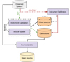 |
Fig. 5. Flow diagram of the flux and LSF calibration process. Dashed arrows show the flow of calibrator data (also the corresponding mean spectra dataset is shown with dashed borders). When applicable the labels INIT or CALONLY have been added to indicate that only data from the corresponding time periods are being used by a given process. |
When calibrations are available to cover the entire time period, a final Source Update using all observed spectra for all sources – not only calibrators – produces the catalogue of mean spectra.
It should be mentioned that in all steps of this process, weighted least squares solutions are obtained via QR-decomposition using Householder reflection to ensure numerical robustness (van Leeuwen 2007). Each solution is computed iteratively: at a given iteration, we use the solution computed at the previous iteration to reject observations that have residuals larger than 5σ. Sample flux measurements are weighted by the inverse variance computed from the flux error for each sample. In the last run of the source update – the one that applies the instrument calibration to all observations to generate the catalogue of mean spectra –, sample flux errors are re-scaled taking into account the scatter in the normalised residuals to mitigate the effects of error underestimation in the wings of the spectra.
3.3.1. Exact solution
Calibrations can also be applied to a single observed spectrum to obtain an internally calibrated epoch spectrum. This process appears as Exact Solution in the schematic overview in Fig. 4. In this case the system of equations to be solved is
 (3)
(3)
where gs is the output internally calibrated epoch spectrum and Ak is the instrument calibration for the calibration unit k of the observed spectrum hs, k being calibrated. In this case, the solution is simply obtained by inverting the matrix representing the instrument calibration and the resulting spectrum has the same sampling (in terms of number of samples and their location in pseudo-wavelength space) as the observed spectrum, as opposed to the mean spectrum that, being defined as a linear combination of some analytic bases, is effectively a continuous function in pseudo-wavelength. The instrument calibration matrix Ak was generally non-singular and the inversion could be done successfully. Only very few epoch spectra could not be calibrated using this procedure.
Epoch spectra are particularly valuable for objects that vary in time (either due to intrinsic variability or due to different distance or orientation such as is the case for Solar System objects). For these types of objects, the mean spectrum will be ill-defined. Although epoch spectra are not included in Gaia DR3, they are relevant here because they have been the input to the generation of the reflectances for Solar System objects.
3.3.2. Calibrations
Calibrations are obtained in time intervals or scopes of about 20 OBMT-Rev (corresponding to about 5 days) for most calibration units. Only for the shortest-exposure configurations, with Gate 05 or Gate 07 active, was it necessary to extend the length of the time intervals to about 100 OBMT-Rev (∼25 days) because of the much smaller number of calibrators in these magnitude ranges. The length of the time intervals will vary slightly between calibrations due to the few events that cause discontinuities in the calibrations (such as decontamination campaigns and refocus events; see also Riello et al. 2021). As within a time scope the calibration is assumed to be constant in time, time scopes need to be defined so that such events happen at the boundary between two subsequent intervals.
A set of calibration parameters was solved for each of the 31 860 calibration units. For Gate 05 and Gate 07, the number of nominal calibration units was 1064 per gate configuration, while for other gate configurations or in the ungated case the number of nominal calibration units was 5708 (the ungated case having twice as many as the others because of the two possible window strategies active for objects with magnitude fainter than 11.5 mag). This implies a total of 24 960 nominal calibration units, but there are often cases of non-nominal configurations that get a sufficient number of observations to allow a robust calibration. These are cases of faint sources being observed with a gate triggered by a nearby bright source being observed at the same time (see also Fig. 2).
Displaying detailed information for such a large number of calibrations is challenging. To facilitate this we define two parameters describing each calibration. One is defined as the sum over j of the Ak(ui, ui + j) values weighted by the distance between ui and ui + j. In the case of a perfectly symmetric calibration (seen here as a convolution kernel) this sum would be equal to zero. In general, it indicates the location of the peak of the kernel. A skewed kernel might be caused by small deviations from the nominal dispersion. The second parameter is given by the sum over j of all Ak(ui, ui + j) values, that is, the integral of the kernel. Variations in this parameter show differences in the response across the focal plane and between different calibration units.
Figure 6 shows an example of the calibration for a given calibration unit, evaluated in the central part of the spectrum and of the CCD. This particular case has the peak parameter equal to −0.80 and the integral parameter equal to 0.98.
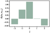 |
Fig. 6. Ak(ui, ui + j) values defining the instrument calibration for one specific configuration (RP, CCD row 1, preceding FoV, ungated, 1D) in the time range including OBMT-Rev 5000 evaluated at ui = 30.0 and AC coordinate 1000. |
The plots shown in Fig. 7 offer a quick view of the calibrations computed for all ungated and 1D configurations for the preceding and following FoVs, in terms of the two parameters defined above. The first row of plots refers to the preceding FoV while the second shows the following FoV calibrations. Starting from left, the first two sets of 14 panels show the variation of the peak parameter with the AL position ui (and therefore wavelength) and time in OBMT-Rev or AC coordinate in all the BP (first seven panels, one panel per CCD) and RP (second column of seven panels) CCDs; the following two sets of 14 panels show the variation of the integral parameter with respect to the same dependencies. Several discontinuities can be observed in the time variation of these parameters. Most of these can be traced back to particular events during the mission, such as decontamination campaigns and refocus activities. The strong variations in the BP calibrations and in particular in the integral parameter versus AL position and time are mostly linked to the varying level of contamination from water-based contaminants present in the payload (Gaia Collaboration 2016), which affects BP more strongly than other instruments (see Fig. 8 in Riello et al. 2018, where the effect of contamination on the photometry in G-band, GBP, and GRP is compared).
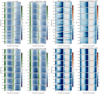 |
Fig. 7. Overview of the BP and RP calibrations for the preceding (first row of plots) and following (second row) FoVs, ungated 1D configuration: peak and integral parameter variations vs. wavelength, time, and AC coordinate are shown for each CCD. Each set of 14 panels show the peak (first two sets) and integral (second two sets) variations (see the top title label and colour bar next to each set) as a function of different parameters: the first set shows the variation of the peak parameter in time (expressed in OBMT-Rev) and pseudo-wavelength, while the second set shows the variation of the same parameter in AC coordinate and pseudo-wavelength, the third and fourth sets show the same dependencies for the integral parameter. When showing the dependency in time and pseudo-wavelength, the parameters have been evaluated at the centre of each CCD in the AC direction (i.e. AC = 1000), while when showing variations with AC coordinate and pseudo-wavelength the reference time OBMT-Rev = 5000 was used. Within each set, the 14 panels show the BP case in the left column of 7 panels (one per CCD) and the RP case in the right column of 7 panels. |
Relative residuals computed for a random subset of the calibrators (about 50 000 sources) are shown in Fig. 8 for BP and RP. For each observed spectrum, relative residuals are computed as the difference between the observed flux value and the predicted value (computed applying the calibration to the source mean spectrum) divided by the observation flux error. Residuals from all observations and all sources in this dataset are accumulated in a grid in ui, magnitude, and colour to analyse residual dependencies. From these plots, it is evident that the performance of the internal calibration for the BP data varies significantly over the wavelength range covered and with magnitude and colour. Sources brighter than G = 12.5 − 13 and in particular red bright sources show a much larger spread in relative residuals. Performances in RP show a much smoother behaviour across all parameters. The additional weights based on the relative frequency of sources in the colour–magnitude diagram (see Sect. 3.2) are likely to be the cause of this. We remind readers that source-based weights were only adopted for the BP calibration to boost the leverage of rare blue sources and to help in the calibration of the bluest wavelength range where only very blue sources have significant flux. This may have affected the calibration process, particularly in magnitude ranges where the number of blue sources is very small because of the natural magnitude and colour distribution of sources in the sky: in these cases, a few blue outliers might adversely affect the solution.
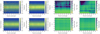 |
Fig. 8. Relative residual distribution for a subset of the calibrators covering the G-band magnitude range [5, 18]. The first row of plots shows the BP results, while the bottom row shows RP. In each row, the first plot shows the distribution of relative residuals vs. AL coordinate in the range [10, 50] where most of the flux is observed. In the second plot, the same distribution is shown including only data from sources in the magnitude range [13, 17]. In these first two plots, the 2D histogram is normalised to the number of measurements in each column and the relative number of sources is shown by the colour bar. The red line shows the median value, while the orange dashed lines show the 15.865 and 84.134 percentiles. The following two plots show the robust width of the distribution of relative residuals defined as the difference between the 84.134 and 15.865 percentiles divided by two vs. G-band magnitude and GBP − GRP colour and AL coordinate for the entire magnitude range covered by this subset. |
The plots in Fig. 8 include only data and calibrations for the INIT period. As explained above, once a stable set of calibrations for the INIT period has been obtained and a reference set of mean spectra for the calibrators is established, these are used to generate consistent calibrations covering all the rest of the mission data collected so far. The distribution in time of the relative residuals covering the whole period included in Gaia DR3 is shown in Fig. 9 for BP and RP in the top and bottom panels, respectively.
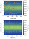 |
Fig. 9. Relative residual distribution for a subset of the calibrators covering the magnitude range [5, 18]. The top panel shows the BP residuals, while the bottom one shows the RP residuals. Only samples with AL coordinate in the range [10, 50] are included in this plot. The 2D histogram is normalised to the number of measurements in each column. |
The top panel shows that the calibration algorithm was not able to fully remove the large systematic effects that are present in the BP data due to the contamination in the early phases of the mission. Considering the long period of time with minimal contamination available, we decided to ignore all BP data collected before the decontamination event that took place shortly before OBMT-Rev 2340 when generating the final catalogue of mean spectra.
3.3.3. Convergence
Convergence of the iterative process was monitored by looking at different parameters: the median standard deviation of the solutions, the overall absolute change in parameters, and the average χ2 of the residuals for a subset of the calibrators were all considered.
Each least squares solution for a calibration unit is assigned a standard deviation. The normalised median standard deviation of all least squares solutions over the OBMT-Rev range [3000, 4000] grouped by gate and window class combination versus iteration number is shown in Fig. 10. Each panel shows a combination of photometer (BP/RP), gate, and window class as indicated in the label. There are some configurations where the evolution of the median standard deviation is not monotonically decreasing, particularly in the first few iterations. If the calibration of each configuration were solved independently, one would expect the corresponding standard deviation to decrease in subsequent iterations. However, in the iterative process described in Sect. 3.3, all calibration units are linked together by the common catalogue of reference spectra that is updated at each source update. For this reason, the fact that the standard deviation does not decrease for all configurations is not a sign of a lack of convergence over all.
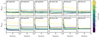 |
Fig. 10. Median standard deviation for all solutions covering the OBMT-Rev range [3000, 4000], normalised to the median standard deviation of all calibrations obtained for the same photometer (BP/RP), gate, and window class at iteration 50 (by that iteration the system seems to have become quite stable). Top panels: BP solutions, one panel per nominal combination of gate and window class. Bottom panels: RP solutions. Different colours indicate different CCD rows and solid and dashed lines are used for the preceding and following FoV, respectively. |
Overall convergence is assessed looking at the absolute relative change in the values of model parameters Ak between two subsequent iterations. Figure 11 shows how these evolve during the iterations for different nominal combinations of gate and window class in BP (top panels) and RP (bottom panels). Given the large number of parameters, only results for ROW4 are shown here, with other rows showing similar trends. The curves in each panel show the median value over the central part of the spectrum in different colours depending on the index j. The overall absolute relative change in calibration parameters is at or below 1% well before iteration 50 for the central part of the spectra and for j = 0. For BP there seem to be larger relative changes (at about the 10% level) in the wings of the spectra and for j ≠ 0. This is not completely unexpected and is probably due to correlations between the parameters.
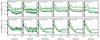 |
Fig. 11. Absolute relative change in the values of model parameters between two subsequent iterations for all solutions covering the OBMT-Rev range [3000, 4000] in a logarithmic scale. The relative change for each parameter is computed as the absolute difference between the values at two subsequent iterations, normalised by the value of the same parameter at the preceding iteration. Top panels: BP solutions, one panel per nominal combination of gate and window class. Bottom panels: RP solutions. Different colours indicate different values of the index j with the darkest line showing j = 0 and lighter colours being used for j = ±1 and j = ±2. The median value over the central part of the spectrum (25.0 < ui < 35.0) is plotted. |
Finally, Fig. 12 shows the evolution through the iterations of the normalised median χ2 for the same random subset of the calibrators used for which residuals where shown in Sect. 3.3. In this plot, the normalised median χ2 value at each iteration is obtained by dividing the corresponding median χ2 by the value at the first iteration. The χ2 value for each epoch spectrum is given as the sum of squared residuals between the observed spectrum and the predicted spectrum divided by the observed flux error. It is important to point out that the normalised median χ2 shown here is not the quantity that is being minimised within the iterative process, which will be the sum of squared residuals for all observations of all calibrators within each calibration unit when solving the instrument model and the sum of squared residuals for all observations of each calibrator when solving the source update step. The increase in late iterations for BP shown in Fig. 12 could be due to changes in the distribution of χ2 caused by the iterations trying to catch a few extreme outliers at the expense of slightly degrading the residuals for other sources.
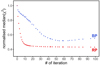 |
Fig. 12. Normalised median χ2 for a subset of about 50 K calibrator sources with respect to the iteration number. Blue and red symbols show the BP and RP residuals, respectively. |
There are indications from both the standard deviation and χ2 analyses that in late iterations the solutions start diverging. We have mentioned a possible cause but this is not fully understood. The additional weighting introduced to give more leverage to blue sources seems to have an effect in this respect. Alternative strategies are being considered for future data releases. From the analysis of all criteria, iterations 55 and 40 were finally adopted for BP and RP, respectively, to proceed with the generation of a reference catalogue of mean spectra to be used for the calibration of the CALONLY data.
3.4. Mean spectra representation
Once the internal reference system has been established by the flux and LSF calibration and calibration solutions are available covering all calibration units, a final source update is run including all observed spectra to generate the catalogue of mean spectra that are released as part of Gaia DR3. The algorithms described in this section have been applied only to this last run of the source update.
3.4.1. Internal reference system
The flux and LSF calibration procedure described in Sect. 3.3 leads to the definition of an internal reference system. This can be seen as an average instrument. The monitoring of intermediate results during the iterative process showed that in late iterations some of the spectral features in mean spectra assumed a smoother, shallower shape with respect to what is observed in the predicted and observed spectra. In order to ensure that the reference system and the corresponding mean spectra remain as close as possible to the actual instrument and to the actual data, we decided to instead use a specific epoch instrument and to represent the final mean spectra as observed in this system. The epoch instrument was chosen somewhat arbitrarily to be the one corresponding to CCD row 7 for BP and row 5 for RP at a time equal to 4500 in OBMT-Rev.
To avoid having to invert the instrument model to derive mean spectra directly in this new system, we computed a transformation matrix T where each row k contains the coefficients that need to be applied to the canonical Hermite function bases to reproduce the prediction of the kth basis in the chosen epoch instrument. These are the result of a fit of each predicted basis function, which is obtained by applying Eq. (1) to a mean spectrum where only one coefficient has a value equal to 1 while all others are 0, with the same set of 55 Hermite function bases. In the new system, the mean spectra are defined by the array of coefficients b′ computed by multiplying the transformation matrix by the array of coefficients in the starting reference system b, that is b′ = T b. The covariance matrix of the source update least squares solution also needs to be converted by computing C′=T C TT where C is the covariance matrix in the starting reference system and C′ is the covariance matrix in the new system.
3.4.2. Bases function optimisation
As described by Carrasco et al. (2021, see Sect. 5) and introduced in Sect. 3.3, the source mean BP/RP spectrum is described as a combination of basis functions. At the start of the calibration process, little is known about the instrument and therefore a generic set of basis functions is used throughout the initialisation phase. Hermite functions, that is, Hermite polynomials multiplied by a Gaussian, were used in this stage: they provide an orthonormal set of basis functions, are centred around zero, and allow to increase details and range by adding higher order bases. These Hermite functions also tend to zero for sufficiently high absolute values of the independent variable. This resembles the behaviour of BP/RP spectra where the combination of CCD efficiency and response ensures that the measured flux tends to zero for increasing distance from the source location.
We denote the n−th Hermite function φn(x). In order to make the Hermite functions efficient in representing the BP/RP spectra, a linear transformation between the pseudo-wavelength and the argument of the Hermite functions is required. This transformation includes a shift Δθ such that the Hermite functions are centred approximately on the centre of the spectra, and a scaling factor Θ that adjusts the width of the Hermite functions to the width of the spectra to be represented. Furthermore, a suitable number of Hermite functions needs to be chosen. The BP/RP spectrum of a source s, fs(u), is then represented by the linear combination
 (4)
(4)
In Eq. (1) the mean spectrum fs(u) appeared as  . Here we have made explicit the transformation of the pseudo-wavelength u into the argument of the Hermite functions φn. The values of Θ, Δθ, and N cannot be chosen independently from each other. Since the pseudo-wavelength range covered by most BP/RP spectra is [0, 60], a value of Δθ of around 30 is required to centre the Hermite functions on the spectra. Furthermore, the linear combination of Hermite functions need to cover the range from −30 to 30. Increasing the number of Hermite functions used in the representation results in the coverage of a wider range of arguments, while increasing the scaling factor results in a reduction of the range of arguments (Carrasco et al. 2021). To find a suitable combination, we first determined the values of N for Δθ = 30 for values of Θ from 2 to 3.5 such that the local minimum or maximum at the largest value of u of the N − 1th basis function is close to 30. For all resulting combinations of Θ and N, a fixed number of five iterations of the instrument calibration was performed. A random subset of approximately 50 000 internal calibrators was used for this purpose. The total residuals in the epoch spectra were then computed and compared for different combinations of parameters. The distribution of the residuals versus various parameters were analysed to select the final combination of parameters. In both BP and RP, N = 55 is used, implying that 55 coefficients will be available for each BP/RP spectrum in Gaia DR3. The values for Θ and Δθ are slightly different for BP and RP, with Θ = 3.062231 for BP and 3.020529 for RP, and Δθ = 30.00986 for BP and 30.00292 for RP. The slight deviation from round numbers is simply the result of adjusting the parameters to the smallest and largest values in pseudo-wavelength in the set of internal calibrators used.
Once the catalogue of mean spectra for the calibrators is established based on the set of standard Hermite functions, the set of bases can be optimised to improve the efficiency of the representation. This is achieved when most of the information is contained in the coefficients for the bases with the lowest indices and allows us to reduce the number of coefficients required to describe each spectrum by dropping coefficients that are within the noise.
The optimisation algorithm used normalised mean spectra for the subset of calibrators already used to define the best configuration for the standard Hermite functions. L2 normalisation was used to ensure equal weights for sources of different magnitude in the decomposition. The N coefficients representing each of these sources in the canonical set of bases are normalised with respect to their l2-norm and are used to populate a matrix M × N where M is the number of sources. Singular value decomposition of this matrix gives the orthogonal matrix V that represents a rotation of the canonical Hermite bases into a new set of optimised bases.
Figure 13 shows the first few bases in the canonical Hermite function set (in the top panel) and in the optimised BP and RP sets of bases (in the following two panels). Darker shades are used for bases with lower indices. The first optimised bases, being tailored to the actual spectra, reproduce the average spectrum and exhibit the imprint of the transmission curve. Higher order bases become increasingly complex with narrower wavy structures required to fit the sharpest features in the spectra.
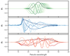 |
Fig. 13. Comparison between the first few canonical Hermite function (top panel), BP (middle panel), and RP (bottom panel) optimised bases. |
3.4.3. Truncation
As explained in Sect. 3.4.2, by expressing the mean spectra in terms of an optimised set of basis functions, a particular spectrum is essentially described by a small number of basis functions with low indices. The coefficients corresponding to higher order basis functions have small absolute values, and, taking their errors into account, are close to zero. Their effect in representing an BP/RP spectrum is therefore essentially adding noise, which manifests itself in wavy structures in the sampled spectrum. It is therefore of interest to suppress the insignificant high-order coefficients and with it, reduce the noise on the spectra.
A simple criterion to decide whether a number of high-order coefficients is insignificant or not has been suggested by Carrasco et al. (2021). The criterion is based on the standard deviation of the M coefficients with the highest indices, that is, the coefficients with indices ranging from N − M to N − 1. All coefficients are normalised by their standard errors. We then compute the standard deviation of the M normalised coefficients with the highest order. If this standard deviation remains below a specified threshold, the M coefficients are considered insignificant. As threshold we use a multiple x of the standard error of the standard deviation. For the standard deviation of a set of M samples from a standard normal distribution we assume the simplified expression of  , and a mean of one. Thus, if the standard deviation of the M normalised coefficients with highest indices is smaller than
  , the coefficients are assumed to be consistent with being zero, and can be truncated. We adopted a value of x = 2, and for each BP/RP spectrum, progressively increasing values of M > 2 were tested for truncation until the standard deviation of the M coefficients exceeds the threshold for some M. If the truncation threshold is never reached, that is, all coefficients are considered to be consistent with being zero, the full number of N = 55 is kept. This happened for a small number of sources, in particular for BP spectra of faint and very red sources, where the flux in the BP spectrum is so low that it is indeed essentially consistent with being only noise.
This criterion makes two simplifications. First, the assumed mean and standard deviation is inaccurate for very small numbers of M. However, the resulting overestimation of the truncation threshold is on the level of a few per cent in the worst case, and has no significant impact on the truncation levels. Second, the truncation ignores correlations between the errors on the coefficients. For sources for which the optimised basis was constructed, the correlations are indeed very low, and the negligence is justified. This is the case for the vast majority of sources. On the other hand, for sources for which the optimised basis is less efficient, correlations might be larger, and the truncation unreliable. This is in particular the case for extremely red sources, or sources with spectral energy distributions that are very different from typical stellar spectral energy distributions, such as quasi-stellar objects (QSOs) or sources with strong emission lines. In the latter case, the truncation is to be used with caution, as it might affect the representation of narrow spectral features.
In the following, we illustrate the effect of truncation for four example cases. First, we consider the case of a typical, bright star (G ≈ 11.5 mag and GBP − GRP ≈ 1.0 mag) in Fig. 14. The top panels compare the sampled BP and RP spectra, represented by all 55 coefficients, and by the number of coefficients considered significant according to the procedure described above. These numbers of coefficients are 35 and 15 for BP and RP, respectively, for this example source. No difference in the sampled spectra is visible to the eye, although the number of basis functions used in the representation of the sampled spectrum is significantly smaller. The bottom panels of the figure illustrate the truncation process. The black symbols show the values of the coefficients normalised to their errors. The red curve shows the standard deviation of the M normalised coefficients, starting from M = 3 on the right-hand side. The blue shaded region is the cone given by  . When the red curve remains below the upper limit of the blue cone, the corresponding higher order coefficients are considered insignificant.
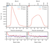 |
Fig. 14. Sampled BP (left) and RP (right) spectra are shown in the top panels for source Gaia DR3 6210089815971933056 (G ≈ 11.5 mag and GBP − GRP ≈ 1.0 mag). Each panel contains two curves: a blue curve showing the non-truncated spectrum using all 55 coefficients, and a red curve showing the truncated spectrum. The number of coefficients used for each spectrum is given in the label within the plot. The bottom panels show the truncation assessment. This is run independently for BP and RP. The black circles indicate the coefficients normalised by their formal errors, and the red line shows the standard deviation of the M normalised coefficients, starting from M = 3 on the right-hand side. The blue shaded region is the cone given by |

The truncation becomes more significant for noisier spectra. As a second example, we therefore consider a source with a similar colour as the first example, but fainter magnitude (G ≈ 18.1 mag and GBP − GRP ≈ 1.0 mag; see Fig. 15). In this case, more coefficients are in agreement with being zero, and the number of significant coefficients is only 2 and 11 for BP and RP, respectively. Truncating the representation of the spectra at these numbers of basis functions maintains the general shape of the spectra, but suppresses the wavy patterns introduced by the noisy higher index coefficients.
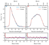 |
Fig. 15. Illustration of the effects of truncation on the mean spectra of source Gaia DR3 6776463197626299392 (G ≈ 18.1 mag and GBP − GRP ≈ 1.0 mag). We refer to the caption of Fig. 14 and the text for details. |
We also show examples for sources with emission lines. The first case is a bright source (G ≈ 11.5 mag) with multiple emission lines in BP and RP, shown in Fig. 16. Here, the truncation criterion is not even reached for M = 3, as all coefficients are required to represent the complex spectra for this source. In similar cases, the number of significant coefficients should have been set to 55, but as the cases where M < =2 were not tested for the truncation criterion, 53 is the maximum number returned by the algorithm. Therefore, the use of all 55 coefficients is recommended in cases where the number of significant coefficients is 53.
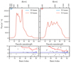 |
Fig. 16. Illustration of the effects of truncation on the mean spectra of source Gaia DR3 3032940844556081408 (G ≈ 11.5 mag). We refer to the caption of Fig. 14 and the text for details. |
Finally, we consider a faint QSO with emission lines as an example. Figure 17 shows the BP and RP spectra of a QSO (G = 18.7 mag and GBP − GRP = 0.5 mag), with all 55 coefficients, and with the truncated representation, using 3 and 11 coefficients in BP and RP, respectively. The spectral energy distribution from SDSS is shown for comparison. In particular, the strong emission line visible in the SDSS spectrum coincides with a line in the BP spectrum. This line is removed by the truncation process. The truncation in the case of complex spectral shapes might therefore be too strong.
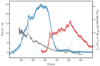 |
Fig. 17. Comparison between the internally calibrated BP (in blue) and RP (in red) spectra vs. the SDSS (in grey) spectrum for QSO Gaia DR3 578415237301611520 (SDSS thing_id = 144680521). Dashed lines are used for the truncated spectra (using only 3 bases for BP and 11 for RP), while continuous lines show the spectra obtained using the full set of 55 coefficients. |
The truncation procedure was also tested by the subsystem dedicated to the estimation of astrophysical parameters within the DPAC analysis pipeline, referred to as Apsis (see Creevey et al. 2023). Most Apsis modules found that the truncation would have a negative impact on the quality of the scientific results based on the emission lines of quasars and certain types of stars. These tests were conducted at a very early stage when no external calibration was available, such that the conclusions were uncertain and most Apsis modules considered not truncating the coefficients to be the safer option. In the extreme case of ultra-cool dwarfs, which are very red and very faint stars, the truncation was found to have a positive impact and has been employed specifically for the Apsis module ESP-UCD which focuses on this type of stars. For these faint stars, the suppression of noise might aid the data analysis.
The result of the truncation assessment is provided as part of the Gaia DR3 in the parameters bp_n_relevant_bases and rp_n_relevant_bases available in the xp_summary table and in the mean continuous spectra available via Datalink (see also Sect. 4). In the case of very faint and typical stars, the use of the truncated representation of BP and RP spectra might be useful. Particularly for sources with unusual spectral energy distributions, such as sources with emission lines, the use of all 55 coefficients for BP and RP, respectively, is advised. The full array of 55 coefficients is available via the archive. Users will need to decide whether or not the suggested truncation is appropriate for their use case.
4. Output data
This Section describes the BP/RP data available via the Gaia archive5. The exact number of sources with BP/RP mean spectra in the Gaia DR3 release is 219 197 643. This list is the result of several selection criteria. Sources with G-band magnitude brighter than 17.65 mag and more than 15 CCD transits contributing to the generation of the mean spectra for both BP and RP were automatically selected. The criterion based on the number of transits leads to a (slightly) non-uniform completeness across the sky (see the density sky distribution in Sect. 7). From this initial list, sources that had shown poor estimates of SSC values (see Sect. 8.2 for more details Riello et al. 2021) were excluded unless they were part of one of the lists of specific objects (see below). An additional 35K sources were excluded to allow further processing and validation within DPAC which is likely to be finalised only after Gaia DR3. A few lists of specific objects for which other criteria would not apply were defined: these included about 500 sources used for the calibration of the BP/RP data, a catalogue of about 100K WD candidates, 17K galaxies, about 100K quasars, about 19K ultra-cool dwarfs, 900 objects that were considered to be the most representative sources (or centroid) for each of the 900 neurons of the self-organising map used by the Outlier Analysis module (Creevey et al. 2023), and finally 19 solar analogues. All these selections are specific to Gaia DR3 and will not affect the content of future releases. In Gaia DR3, there is one source (Gaia DR3 5405570973190252288) that has only an RP spectrum.
The gaia_source table in the archive contains a boolean column has_xp_continuous that is true if the corresponding source has BP/RP mean spectra available6. After retrieving a list of gaia_source entries, BP/RP spectra can be downloaded from the archive via Datalink7 in various file formats. This can be done either from the archive web interface or programmatically. In Appendix A we provide instructions for downloading the data from Python.
The spectra are provided in the continuous representation (see also Appendix B for more details): for each BP and RP, the spectrum is defined as a set of coefficients (bp/rp_coefficients); an array with the coefficient formal errors, defined as the standard uncertainties from the least square solution multiplied by the standard deviation of the solution (bp/rp_coefficient_errors); the correlation matrix8 (bp/rp_coefficient_correlations); various parameters from the source update process, such as number of measurements, number of degrees of freedom, χ2 and standard deviation of the solution.
In addition to the data available via Datalink, the xp_summary table provides access to some of the parameters listed in the previous paragraph via queries (e.g., to enable the selection of sources based on the standard deviation of their mean spectrum solution) and to other relevant information. Users interested in retrieving the number of CCD transit spectra (and individual measurements) that contributed to the generation of the mean spectrum or that want to know how many of these were assessed as contaminated or blended should interrogate this table, not the main gaia_source table which instead provides similar counters for the photometric data. While BP/RP spectra and G-band and BP/RP photometry share part of the processing and filtering criteria, there are also some important differences that can lead to apparent inconsistencies in these counters.
The Python package GaiaXPy9 has been developed to help the users of BP/RP spectra. It offers the following functionalities: generation of a sampled version of the original continuous representation in both internal and absolute flux and wavelength systems, computation of synthetic photometry in various photometric systems and simulation of Gaia-like mean spectra from an input absolute spectral energy distribution. For more information on these tools, we refer to the online package documentation.
5. Validation
5.1. Errors
In order to test the performance of the calibration, a special validation dataset was generated where for each source the available transits were randomly divided into two groups and processed separately to generate two mean spectra for BP and two for RP. This allows us to compare the calibration results from two sets of transits for the same sources. We refer to this dataset as the BP/RP split-epoch validation dataset. Further details (including how to access the dataset) are available in Appendix D.
For this comparison, we computed the Mahalanobis distance, DM between the two solutions for each source, given by
 (5)
(5)
Here, c1 and c2 denote the coefficient vectors for the two solutions, and Σ1 and Σ2 the corresponding covariance matrices. Under the idealised circumstances of normally distributed noise, correct covariance matrices, and the absence of intrinsic photometric variability of the sources used in the test, DM follows a chi distribution with the degree of freedom corresponding to the length of c1 and c2. Deviations from a chi distribution therefore indicate unreliable covariance matrices Σ1 or Σ2.
We analysed the distribution of the DM in comparison to the chi distribution as a function of colour, magnitude, and indices of coefficients. The dependency on colour is only weak, with slightly larger values of DM for very red sources, with GBP − GRP ≳ 3.0 mag. The magnitude dependency is more pronounced, and depends on the indices of the coefficients. This is illustrated in Fig. 18. The top panels of this figure show the distribution of the DM, normalised to the total number of sources in each magnitude bin, for all 40K test sources, for the first five and the last five coefficients in BP, respectively. For the first five coefficients, the values of DM are in general too large compared to what is expected from a chi distribution, an effect that is more pronounced for bright sources. For the five coefficients corresponding to the highest order basis functions, the magnitude dependency is weaker, with values being slightly smaller than expected from a chi distribution for the brighter sources.
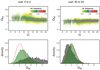 |
Fig. 18. Top panels: distribution of the Mahalanobis distances of all test sources as a function of G-band magnitude. The grey horizontal line indicates the mean of the chi distribution. Bottom panels: histograms of the Mahalanobis distances for sources with G < 10 mag (grey) and G > 16 mag (green). The red line is the corresponding chi distribution. The left-hand side plots are for the first five coefficients, with indices 0–4, and the right-hand side plots are for the five coefficients of highest order, with indices 50–54. |
The bottom panels of Fig. 18 show the density histograms for bright sources, with G < 10 mag in grey, and faint sources, with G > 16 mag in green, respectively, in comparison with the chi distribution for five degrees of freedom. For the first five coefficients, the distribution is much wider than the chi distribution, in particular for the bright sources, and is shifted to larger values. For the last five coefficients, the faint sources are in good agreement with a chi distribution, while the distribution for the bright sources is shifted towards smaller values of DM.
An underestimation of the error results in larger DM than expected from a chi distribution, while an overestimation of the error results in smaller values. The differences in DM with respect to the chi distribution can therefore be interpreted as an underestimation of the errors for the coefficients with low indices, and an overestimation of the errors for coefficients of high indices for bright sources. For high indices and faint sources, the errors are however reliable. While the results shown here are from BP spectra, the situation for RP is similar. When using the BP/RP spectra, the errors for brighter sources in particular should be interpreted with caution.
5.2. Specific cases
Although most of the spectra show a good behaviour, there are a few cases where we see peculiar shapes, which are due to several factors. In the following, we analyse a few of the most common situations.
In the case of very faint sources, the fitting procedure generating the mean spectrum will be poorly constrained and may produce unrealistic features. For example, Fig. 19 shows the spectra of a faint red source (with GBP = 21.6 mag and GRP = 17.8 mag). For this type of spectrum, the parameters bpnrelevantbases and rpnrelevantbases in the xpsummary table in the Gaia DR3 archive are particularly relevant, as they indicate the number of coefficients that are significant considering the noise level (see Carrasco et al. 2021, and Sect. 3.4.3 in this paper for more details). In this case, only 1 of the 55 coefficients defining the BP spectrum is considered significant. Our adopted truncation procedure suggests that, for BP, all coefficients beyond the first one are only fitting the noise fluctuations rather than real spectral features and can be ignored when using the mean spectra for further investigations. For RP, the number increases to 11 thanks to the higher S/N.
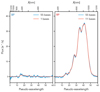 |
Fig. 19. BP (left) and RP (right) spectra for the faint red source Gaia DR3 1252666141462905344 (GBP = 21.6 mag and GRP = 17.8 mag). The blue curves show the spectra defined by the 55 coefficients (errors are shown as a shaded area). The red curves show the truncated spectra where only the first bp/rp_n_relevant_bases have been used. |
In crowded areas, it is possible that two or more sources are so close in the sky that their observations are always or often contaminated or blended. We refer to blended spectra when two or more sources fall within the observed window, while contamination refers to flux belonging to a source that is located outside the window. If this happens in a large fraction of the observations of a given source, then the mean spectra for that source will be affected. To enable users to assess the reliability of BP/RP mean spectra, the xpsummary table in the archive includes several parameters (bp/rpnblendedtransits and bp/rpncontaminatedtransits) indicating the number of transits affected by blending or contamination for all sources for which BP/RP spectra are published. Figure 20 shows the case of four sources in the globular cluster 47 Tuc that have all their observations flagged as blended. Users are strongly encouraged to make use of the available crowding flags to detect problematic cases.
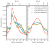 |
Fig. 20. BP (left) and RP (right) normalised internal spectra of some sources with all transits blended by other nearby sources in the 47 Tuc cluster. |
The wings of the spectra should normally have a low flux level because of the combined action of LSF, dispersion, and response. However, this may not be the case because of the presence of residual background flux not fully removed in the background calibration stage or diffused flux due to the source being extended. For example, Fig. 21 shows the BP and RP internal spectra for a source with the ingalaxycandidates flag in the gaiasource table set to true. Both spectra present a higher-than-normal flux in the wings. This source also shows a significant mismatch between the photometry in the different bands (G = 18.7 mag, GBP = 15.7 mag and GRP = 14.3 mag), the two BP/RP integrated flux values being much brighter than the value in the G-band, due to the much larger size of the BP/RP windows with respect to the AF ones.
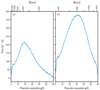 |
Fig. 21. BP (left) and RP (right) internally calibrated spectra of a source (Gaia DR3 1252344813484742272) flagged as galaxy in the gaia_source table. The spectra are broader than expected and the corresponding integrated magnitudes are much brighter compared with the G-band photometry. |
A similar effect is seen when considering objects that are close to a very bright source. Their spectra will appear to be contaminated by flux coming from the nearby bright object. The resolution of the background calibration is not sufficient to completely remove this effect and may actually lead to an under- or overestimation of the background in the regions surrounding very bright sources. Figure 22 shows the BP/RP spectra for two sources near Sirius. Source Gaia DR3 2947050466531872640, at 30 arcsec from Sirius, is clearly contaminated by diffuse flux coming from the nearby bright source. Also in this case, the photometry indicates a much brighter source in the BP/RP integrated bands than in the G-band: G = 15.7 mag, GBP = 13.2 mag, and GRP = 13.2 mag. The second source (Gaia DR3 2947047202356748672) is located further away at about 3 arcmin. In this case, the background seems to have been overestimated, causing negative flux values in the wing of the spectra in both BP and RP.
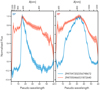 |
Fig. 22. BP (left) and RP (right) internally calibrated spectra of two sources near Sirius: one located at 30 arcsec (in red) and the other at 3 arcmin (in blue). The source closest to Sirius shows clear signs of contamination from the nearby object. |
5.3. Signal-to-noise ratio
An overall indication of the S/N for a given source and photometer can be obtained directly from the coefficients by dividing the L2-norm of the vector of coefficients by the L2-norm of the vector of errors on the coefficients. Figure 23 shows a colour–magnitude diagram of the sources with BP/RP spectra in Gaia DR3 colour coded by this global S/N in the BP and RP photometers in the left and right panel.
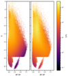 |
Fig. 23. Colour–magnitude diagram of a random 10% of the sources for which BP/RP spectra are available in Gaia DR3, colour coded in a logarithmic scale by the global S/N as computed directly from the continuous representation coefficients and their errors. BP and RP S/Ns are shown in the left and right panels, respectively. |
A user that is interested in the S/N at different wavelengths will have to consider the representation of the spectrum by the linear combination of basis functions that have an explicit wavelength dependency rather than relying on the coefficients alone. The panels in Fig. 24 show typical S/N distribution of internally calibrated spectra over the BP (left panels) and RP (right panels) pseudo-wavelength ranges covered by the BP/RP spectra. In the top two panels, each curve shows the S/N for sources of different magnitude, as reported in the colour bar, GBP − GRP colour close to 1.0, and with typical global S/N (for sources of similar magnitude and colour). In the bottom two panels instead, each curve shows the S/N for sources of different colour, as reported in the colour bar, G-band magnitude close to 16.0 and with typical global S/N (for sources of similar magnitude and colour). Only sources with |c*|< 0.02 have been considered for these plots, c* being the corrected BP/RP flux excess factor as defined in Riello et al. (2021). As in previous figures, the top axes showing the correspondence with absolute wavelengths are only indicative.
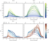 |
Fig. 24. S/N vs. pseudo-wavelength (and approximate absolute wavelength) for internally calibrated spectra. The top panels show the S/N for sources of different magnitude and similar colour (close to 1.0), while the bottom panels focus on sources with similar G-band magnitude (close to 16.0) and a range of colours. |
Due to the fact that the mean BP/RP spectra are a combination of many single observations for each object, intrinsic variability will result in larger uncertainties in the mean spectra. This is confirmed by the fact that the S/N for a sample of known RR Lyrae (extracted from Clementini et al. 2023) is significantly lower than the S/N for a sample of random (mostly non-variable) sources with similar apparent G.
The dependency of the S/N from pseudo-wavelength is linked to the spectrum itself. Looking at the top-right panel of Fig. 24, the maximum S/N in RP is achieved for sources with G 9–10. Saturation and occasional gate misconfiguration could be responsible for this: while the mean spectra of very bright sources do not show clear signatures of saturation, the presence of some saturated epoch spectra among those contributing to the mean spectrum –which is possibly due to gate misconfiguration caused by large on-board magnitude errors at the bright end– could lead to a larger scatter around the peak and therefore a larger error and a lower S/N than expected.
6. Recommendations
6.1. Recommended format
The mean spectra are available in the archive in the form of a set of coefficients that define a continuous function over the pseudo-wavelength range. This is the fundamental product of the BP/RP spectral data processing. When sampling the spectra on a discrete grid in pseudo-wavelength (or wavelength if working in the absolute system), some information is unavoidably lost. In particular, the continuous representation comes with full covariance information, whereas a spectrum sampled on a (pseudo-)wavelength grid with more points than the number of coefficients in the continuous representation cannot. Users are therefore strongly encouraged to consider using the continuous representation to best exploit the BP/RP spectra in Gaia DR3 (e.g., to derive astrophysical parameters or analyse the presence of spectral features) and avoid sampling the spectra or deriving synthetic photometry from them, losing information in the process.
Figure 25 shows that the coefficients can be used to successfully classify sources in different regions of the Hertzsprung–Russell diagram. At least for the few cases shown in the plot, most of the information required for classification is already available in the first few coefficients of the continuous representation. Figure 26 shows the corresponding plot with the more familiar sampled spectra.
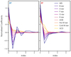 |
Fig. 25. First eight coefficients of the continuous representation in BP (left) and RP (right) for some sources with different astrophysical parameters. |
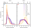 |
Fig. 26. Normalised internal mean spectra in BP (left) and RP (right) for the same sources shown in Fig. 25. |
Figure 13 clearly shows that narrow spectral features in the spectra can only be reproduced with larger higher order coefficients. For example, Fig. 27 shows an example of two sources with rather similar RP spectra except for the presence of a strong emission line. One of the two sources is a QSO. As can be seen in the bottom right panel, higher order coefficients for the QSO have larger values.
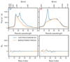 |
Fig. 27. Comparison of the mean spectra obtained for a QSO with a strong emission line (Gaia DR3 1255795527649038720 in blue), and another source with similar shape and flux level but without strong features (Gaia DR3 4689627408431598336 in orange). BP and RP are shown in the left and right panels, respectively. Sampled spectra are shown in the top panels, while the bottom panels show the corresponding coefficients. |
6.2. Effects of noise
The correlations between the coefficients of a source, both for BP and RP, are in general rather low, with median correlation coefficients well below 0.1 in both BP and RP. When constructing the sampled spectrum as a function of pseudo-wavelength (or wavelength), the correlations might become much more important. As there are only 55 basis functions for BP and RP, respectively, any sampled spectrum with more than 55 sample points needs to have linear dependencies among the samples. Furthermore, even if the coefficients were uncorrelated, the non-local character of the basis function representation would still introduce correlations between different pseudo-wavelengths. This effect is illustrated in Fig. 28 for the RP spectrum of one particular source, with G = 17.89, GBP − GRP = 2.74. The BP/RP split epoch validation dataset (see Appendix D) has been used for this analysis. The two sets of transits for this source contain 18 transits and 3 transits, respectively. Consequently, the S/N in the first set is higher than in the second one. This is seen in the first column of Fig. 28, where the coefficients for the calibration using only three transits are noisier and have larger error bars than for the 18 transits case. The second column in this figure shows the correlation matrices for the two cases. In general the correlations are low, with little structure in the off-diagonal entries. However, the correlations are larger for the noisier case. The third column shows the sampled RP spectra for the 18 transits and the three transits cases. The larger noise in the latter case manifests itself in a wavy structure in the sampled spectrum. In the correlation matrix for the sampled spectrum, shown in the fourth column, this larger noise manifests itself in the form of alternating short-scale patterns of positive and negative correlations. These patterns are again more pronounced when the S/N is lower. As random noise in the BP/RP spectra manifests itself in the sampled spectra as wavy structures, and correlations within the sampled spectra are not negligible, the interpretation of the coefficients, being much less affected by correlations, might be more convenient.
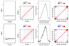 |
Fig. 28. Example of the effect of noise for an RP spectrum. First column: RP coefficients with errors. Second column: correlation matrices for the coefficients. Third column: sampled RP spectrum (black line) with 1-sigma uncertainty interval (grey shaded region). Fourth column: correlation matrix for the sampled RP spectrum. The top row is for 18 transits, and the bottom row for 3 transits, for the same source. |
7. Conclusions
In this paper, we focus on the processing that generated the internally calibrated BP/RP spectra contributing to Gaia DR3 starting from the raw satellite data. The released data are time-averaged source spectra that result from the combination of all single observations of a given source. Only a selection of all generated spectra will be included in the release at this stage, but several other new products are based on the entire dataset. The main challenges faced by this step in the data processing are due to the vast amount of data (about 65 billion single BP/RP transits were processed), to the nature of the low-resolution aperture prism spectroscopy with the additional complications added by the TDI mode, and to the large number of different observing configurations effectively corresponding to the different instruments that need to be calibrated onto the same homogeneous system. We explain how we dealt with these challenges and show how we have been monitoring the intermediate performances of our calibration procedures. We also describe the somewhat unfamiliar format of the BP/RP spectral data in the archive. Rather than providing spectra defined as a flux value corresponding to a sample covering a given wavelength range, the BP/RP spectra are represented by an array of coefficients, and their errors and correlations, which are to be applied to a set of basis functions to obtain a continuous function. This approach allows us to combine multiple transit spectra, each having its own sampling, dispersion, and LSF (Carrasco et al. 2021). The set of bases has been optimised to ensure maximum efficiency, thus focusing most of the flux in the first few coefficients and leaving higher order coefficients to be constrained by narrow spectral features.
We want to conclude this paper by showing some sky distributions related to the BP/RP data in Fig. 29. All maps are in Galactic coordinates and show the entire catalogue of sources with BP/RP spectra in Gaia DR3. The first map shows the density distribution in the sky. As expected, most of the sources are concentrated along the Galactic plane. The two Magellanic Clouds also stand out, as well as a few clusters. The darkest areas close to the Galactic plane in the map correspond to regions obscured by dust and regions with extremely high density where the BP/RP data are particularly affected by strong crowding (both in the acquisition and in the processing). Some regions with lower density away from the Galactic plane still show imprints of the scanning law (compare this with the map showing the median number of transits). These are expected to disappear with the addition of more observations in future releases. The second map shows the distribution of GBP − GRP colour. The third map shows the median number of transits per source (in RP). This is clearly defined by the satellite scanning law. A similar map of BP would be very similar with the exception of the occurrences of a larger number of transits near the Ecliptic poles. These are due to the first month of operations in Ecliptic scanning law. This period was not included in the generation of average source BP spectra as explained in Sect. 3.3. The fourth map shows the median fraction of contaminated or blended transits with respect to the number of transits per source for RP. The equivalent maps for BP would be very similar. The areas showing higher density in the first map also stand out in this map as regions where the mean spectra are more affected by crowding. This is justified by the fact that the crowding evaluation is limited to the Gaia source catalogue itself. Finally, the last two maps show the distribution in the sky of the median of the 84th percentile of the S/N distribution over the BP and RP wavelength ranges. As expected, the scanning law signature is very evident in these maps with errors being lower in the most observed regions. Areas at low Galactic latitude show lower S/N in the BP spectra due to the abundance of red-coloured sources. The S/N distribution of the internally calibrated spectra shows values larger than 1000 for bright sources in some wavelength ranges (see Fig. 24). Gaia DR3 will contain about 700 000 BP spectra and 4.3 million RP spectra with the 84th percentile of the S/N above 500.
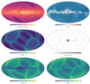 |
Fig. 29. Sky distribution (in Galactic coordinates in Hammer-Aitoff projection, with resolution equivalent to HEALPiX level 7) of various parameters related to the BP/RP data: from the top left to the bottom right the maps show the sky density of objects with BP/RP spectral data, the median GBP − GRP colour, the median number of transits in RP contributing to the mean spectra, the median crowding level, and the median of the 84th percentile of the S/N over the BP and RP ranges. The colour scales do not cover the full range covered by the data. |
Various parameters available from the archive can be useful to clean the catalogue from disturbed spectra. A very useful quantity already introduced for Gaia DR2 is the phot_bp_rp_excess_factor. This parameter is available from the gaia_source table and is defined as the ratio between the sum of BP and RP integrated fluxes and the G-band flux for the same source. Due to the shape of the G, GBP, and GRP passbands, some colour dependency of this ratio is expected and may bias selections based on phot_bp_rp_excess_factor. To correct for the expected colour trends, users should apply the equation recommended in Riello et al. (2021) to form what is known as C⋆ 10. The deviation of this parameter from 0.0 indicates the presence of inconsistencies between the flux measured in the BP/RP windows and the flux in the G-band. These inconsistencies can be due to different source properties (e.g., in the case of extended sources) or systematic errors in the calibration procedures (e.g., in the case of residual background due to nearby bright sources). Section 9.4 in Riello et al. (2021) also provides a function reproducing the 1σ scatter for a sample of well-behaved isolated stellar sources with good-quality photometry. Users wishing to use C⋆ and its 1σ scatter to select the most reliable spectra would find that 90% of the sources have C⋆ < 3σ while 79% fulfil the criterion C⋆ < 1σ. Figure 30 shows the distribution of C⋆ together with the 1- and 3-σ limits.
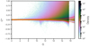 |
Fig. 30. Distribution of C⋆ vs. magnitude for all sources with BP/RP spectra in Gaia DR3. Also shown are the 1- and 3-σ curves in yellow and red, respectively, as defined in Riello et al. (2021). |
In terms of BP/RP spectral data, future releases will see a vast increase in the number of average source spectra and the addition of calibrated epoch spectra, that is, spectra derived from one single observation in BP/RP. From a processing and validation point of view, this will focus the attention on calibrations that deviate from the average behaviour. While robust techniques help mitigate these problems when generating mean spectra, the application of noisy calibrations can generate unreliable data. This needs to be mitigated to ensure the quality of calibrated BP/RP epoch spectra, which we plan to include in future releases. One other area where some improvement is being sought is in the bluest wavelength range covered by BP (350 − −400 nm) where the small fraction of calibrators makes the flux and LSF calibration particularly challenging. The effect of this can be seen in some systematic offsets in the bluest part of the wavelength range covered by BP/RP data. These can be quantified when comparing BP/RP spectra with external absolute spectra (Montegriffo et al. 2023) and/or synthetic photometry generated from BP/RP spectra in various bands and photometric systems versus existing catalogues (Gaia Collaboration 2023c). In particular, in the latter work, the comparison of synthetic photometry from externally calibrated BP/RP spectra with state-of-the-art ground-based photometric standard stars suggests that, in the wavelength range spanned by SDSS u-band (and/or Johnson-Kron-Cousins U), differences can be as large as 20% for some spectral types and in some colour ranges. In the range covered by SDSS g-band (and/or Johnson-Kron-Cousins B-band), systematic errors reach the 5% level at most, while for redder passbands they are typically below the 2% level.
See the list of refereed papers since launch available at https://ui.adsabs.harvard.edu/public-libraries/fWFE_JYLRZG2jwgwKetH8w
The angular dimensions of each pixel are approximately 58.9 and 176.8 mas in the AL and AC directions, respectively.
When querying the gaia_source table for sources fulfilling some criteria and having BP/RP spectra available, the user needs to add WHERE has_xp_continuous=‘true’ to the ADQL query.
See https://www.cosmos.esa.int/web/gaia-users/archive/ancillary-data
Given the symmetry of the correlation matrix, only the upper triangular elements (above and not including the diagonal elements which are 1 by definition) of the matrix are provided. The matrix elements are stored as a 1D array of size n (n − 1)/2 where n is the number of coefficients. The full correlation matrix would therefore be of size n × n. The ordering of the elements in the array follows a column-major scheme.
C⋆ is obtained from the phot_bp_rp_excess_factorC as C − f(GBP − GRP) where f(GBP − GRP) is a polynomial in colour defined as
where x = GBP − GRP.
The corrected parameter (c_star) will be available for all sources included in the Gaia Synthetic Photometric Catalogue from the archive; see Gaia Collaboration (2023c).
https://doi.org/10.5281/zenodo.6799330
https://doi.org/10.5281/zenodo.6802733
Acknowledgments
We are very grateful to the anonymous Referee for a careful and constructive report, that improved the quality of the manuscript. We would also like to thank R. Blomme for kindly reviewing an earlier version of this manuscript. This publication made extensive use of the online authoring Overleaf platform (https://www.overleaf.com/). The data processing and analysis made use of matplotlib (Hunter 2007), NumPy (Harris et al. 2020), the IPython package (Pérez & Granger 2007), TOPCAT (Taylor et al. 2005). This work presents results from the European Space Agency (ESA) space mission Gaia. Gaia data are being processed by the Gaia Data Processing and Analysis Consortium (DPAC). Funding for the DPAC is provided by national institutions, in particular the institutions participating in the Gaia MultiLateral Agreement (MLA). The Gaia mission website is https://www.cosmos.esa.int/gaia. The Gaia archive website is https://archives.esac.esa.int/gaia. Full acknowledgements are given in Appendix F.
References
- Akeson, R., Armus, L., Bachelet, E., et al. 2019, ArXiv e-prints [arXiv:1902.05569] [Google Scholar]
- Altavilla, G., Marinoni, S., Pancino, E., et al. 2021, MNRAS, 501, 2848 [NASA ADS] [CrossRef] [Google Scholar]
- Altavilla, G., Marinoni, S., Pancino, E., et al. 2015, Astron. Nachr., 336, 515 [NASA ADS] [CrossRef] [Google Scholar]
- Andrae, R., Fouesneau, M., Sordo, R., et al. 2023, A&A, 674, A27 (Gaia DR3 SI) [NASA ADS] [CrossRef] [EDP Sciences] [Google Scholar]
- Babusiaux, C., Fabricius, C., Khanna, S., et al. 2023, A&A, 674, A32 (Gaia DR3 SI) [NASA ADS] [CrossRef] [EDP Sciences] [Google Scholar]
- Carrasco, J. M., Evans, D. W., Montegriffo, P., et al. 2016, A&A, 595, A7 [NASA ADS] [CrossRef] [EDP Sciences] [Google Scholar]
- Carrasco, J. M., Weiler, M., Jordi, C., et al. 2021, A&A, 652, A86 [NASA ADS] [CrossRef] [EDP Sciences] [Google Scholar]
- Clementini, G., Ripepi, V., Garofalo, A., et al. 2023, A&A, 674, A18 (Gaia DR3 SI) [NASA ADS] [CrossRef] [EDP Sciences] [Google Scholar]
- Costille, A., Caillat, A., Rossin, C., et al. 2016, SPIE Conf. Ser., 9912, 99122C [Google Scholar]
- Creevey, O. L., Sordo, R., Pailler, F., et al. 2023, A&A, 674, A26 (Gaia DR3 SI) [NASA ADS] [CrossRef] [EDP Sciences] [Google Scholar]
- Dean, J., & Ghemawat, S. 2008, Commun. ACM, 51, 107 [CrossRef] [Google Scholar]
- Evans, D. W., Eyer, L., Busso, G., et al. 2023, A&A, 674, A4 (Gaia DR3 SI) [NASA ADS] [CrossRef] [EDP Sciences] [Google Scholar]
- Fabricius, C., Bastian, U., Portell, J., et al. 2016, A&A, 595, A3 [NASA ADS] [CrossRef] [EDP Sciences] [Google Scholar]
- Gaia Collaboration (Prusti, T., et al.) 2016, A&A, 595, A1 [NASA ADS] [CrossRef] [EDP Sciences] [Google Scholar]
- Gaia Collaboration (Galluccio, L., et al.) 2023a, A&A, 674, A35 (Gaia DR3 SI) [NASA ADS] [CrossRef] [EDP Sciences] [Google Scholar]
- Gaia Collaboration (Vallenari, A., et al.) 2023b, A&A, 674, A1 (Gaia DR3 SI) [NASA ADS] [CrossRef] [EDP Sciences] [Google Scholar]
- Gaia Collaboration (Montegriffo, P., et al.) 2023c, A&A, 674, A33 (Gaia DR3 SI) [CrossRef] [EDP Sciences] [Google Scholar]
- Harris, C. R., Millman, K. J., van der Walt, S. J., et al. 2020, Nature, 585, 357 [NASA ADS] [CrossRef] [Google Scholar]
- Hunter, J. D. 2007, Comput. Sci. Eng., 9, 90 [NASA ADS] [CrossRef] [Google Scholar]
- Jordi, C., Høg, E., Brown, A. G. A., et al. 2006, MNRAS, 367, 290 [NASA ADS] [CrossRef] [Google Scholar]
- Marinoni, S., Pancino, E., Altavilla, G., et al. 2016, MNRAS, 462, 3616 [Google Scholar]
- Montegriffo, P., De Angeli, F., Andrae, R., et al. 2023, A&A, 674, A3 (Gaia DR3 SI) [NASA ADS] [CrossRef] [EDP Sciences] [Google Scholar]
- Pancino, E., Sanna, N., Altavilla, G., et al. 2021, MNRAS, 503, 3660 [Google Scholar]
- Pérez, F., & Granger, B. E. 2007, Comput. Sci. Eng., 9, 21 [Google Scholar]
- Pickering, E. C. 1890, Ann. Harvard College Obs., 27, 1 [Google Scholar]
- Riello, M., De Angeli, F., Evans, D. W., et al. 2018, A&A, 616, A3 [NASA ADS] [CrossRef] [EDP Sciences] [Google Scholar]
- Riello, M., De Angeli, F., Evans, D. W., et al. 2021, A&A, 649, A3 [NASA ADS] [CrossRef] [EDP Sciences] [Google Scholar]
- Taylor, M. B. 2005, ASP Conf. Ser., 347, 29 [Google Scholar]
- van Leeuwen, F. 2007, Hipparcos, the New Reduction of the Raw Data, 350 (Dordrecht: Springer) [Google Scholar]
Appendix A: Downloading BP/RP data from the Gaia DR3 archive
Not all sources included in Gaia DR3 will have BP/RP spectra available. The main gaia_source table in the archive contains a field has_xp_continuous that is true if a BP/RP spectrum is available for that source. Users can therefore query the gaia_source table to select sources with their favourite combination of parameters and use the additional criterion has_xp_continuous=’true’ to restrict their selection to sources that have BP/RP spectra available from the archive.
The support of the Datalink feature in the archive includes an independent service for the serialization of the BP/RP spectra. Other types of data such as photometric light curves are served using similar services. A dedicated tutorial is available https://www.cosmos.esa.int/web/gaia-users/archive/ancillary-datatutorialdatalinklc.
In this section we provide an example of how to download BP/RP spectra using the Python programming language. By splitting the list of sources identifiers (ids[’source_id’] in the following code snippet), users can overcome the Datalink limitation on the number of sources. A bulk download option will also be implemented for users interested in getting all the BP/RP spectra in Gaia DR3.
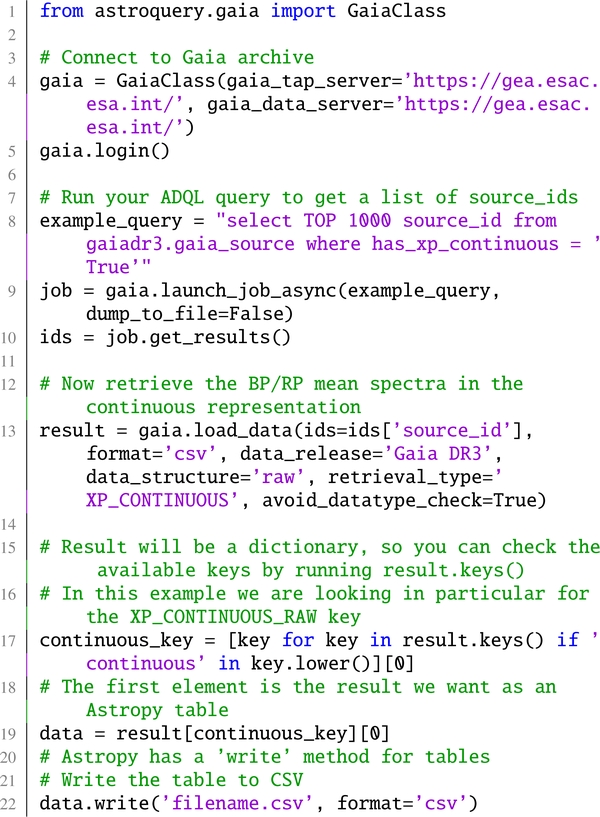
The data can be downloaded in different file formats. For a complete list of the available formats and for instructions on alternative download procedures, please refer to the archive pages and tutorials.
Once downloaded, the files can be given in input to GaiaXPy utilities to obtain sampled spectra or synthetic photometry. GaiaXPy also offers the possibility of providing a list of source IDs. In this case, the download of the spectra from the archive is done within the GaiaXPy utility (users will be prompted for credentials).
Appendix B: Data format details
This section provides more detailed information on the structure of the data representing BP/RP mean spectra in the archive. For completeness, all fields are described here, even though some have been mentioned and explained in the main text. Detailed descriptions are also available from the Gaia DR3 documentation and from the archive documentation.
We first describe the fields available via DataLink when retrieving XP_CONTINUOUS data:
-
source_id Source identifier. Among other information, this encodes the approximate position of the source in the equatorial system (ICRS) using the nested HEALPix scheme at level 12 (Nside = 4096), which divides the sky into ≃200 million pixels of about 0.7 arcmin2.
-
bp/rp_basis_function_id Identifier of the set of bases functions used in the Source Update process (see Sect. 3.3). Different sets were used during trial runs and validation but all the released spectra were created using the same set of bases. This implies that the identifier in Gaia DR3 is different for BP and RP spectra, but the same for all sources in each band. When sampling the spectra in the internal reference system, care must be taken to ensure that the right basis configuration is used.
-
bp/rp_degrees_of_freedom Number of degrees of freedom in the Source Update least squares solution.
-
bp/rp_n_parameters Number of parameters in the Source Update least squares solution. This will be always 55 for the Gaia DR3 BP/RP spectra.
-
bp/rp_n_measurements Number of measurements contributing to the Source Update least squares solution. This counts the single samples contributing rather than full epoch spectra.
-
bp/rp_n_rejected_measurements Number of samples rejected in the Source Update least squares solution. This is based on a k-sigma rejection algorithm.
-
bp/rp_standard_deviation The final standard deviation of the Source Update least squares solution for this BP/RP and source.
-
bp/rp_chi_squared The χ2 of the Source Update least squares solution for this BP/RP and source.
-
bp/rp_coefficients The array of coefficients of the mean spectrum representation as a superposition of basis functions. These are the bs, n in Eq. 4. This array will have length equal to bp/rp_n_parameters.
-
bp/rp_coefficient_errors The errors on the coefficients, one error per coefficient. This array will have length equal to bp/rp_n_parameters. The errors in this array are computed multiplying the formal errors (as obtained from the covariance matrix of the source update least square solution) by the standard deviation of the solution. This is a standard methodology and can also account for when the modelling of the data introduces a systematic error that adds a pseudo-random error to the individual input data not accounted for in quoted errors.
-
bp/rp_coefficient_correlations The matrix containing the information on correlations between coefficients. Only the elements located in the upper triangular section of the matrix, excluding the diagonal where all elements are equal to 1.0 by definition, are stored as an array of constant size n (n − 1)/2 where n is equal to bp/rp_n_parameters. The order of the elements in the linear array follows a column-major scheme, i.e. for n = 55,
![Mathematical equation: $$ \mathbf{M} = \begin{bmatrix} 1&C[0]&C[1]&C[3]&C[6]&\cdots&C[1431]\\&1&C[2]&C[4]&C[7]&\cdots&C[1432]\\&1&C[5]&C[8]&\cdots&C[1433]\\&&1&C[9]&\cdots&C[1434]\\&&1&\cdots&\vdots \\&&&1&C[1484]\\&&&1 \\ \end{bmatrix} $$](/articles/aa/full_html/2023/06/aa43680-22/aa43680-22-eq13.gif)
-
bp/rp_n_relevant_bases Number of coefficients that were considered above the noise according to the criterion described in Sect. 3.4.3.
-
bp/rp_n_relative_shrinking Ratio between the L2-norm of the truncated and full BP/RP spectrum.
In the following, we also describe the additional fields available in the xp_summary table (fields that duplicate information given in the above data structure are not repeated here):
-
bp/rp_n_transits Number of epoch spectra contributing to the mean spectrum.
-
bp/rp_n_contaminated_transits Number of transits assessed as contaminated among those that contributed to the mean spectrum. A transits is considered contaminated when some of the flux within the window is estimated to come from a nearby (on the focal plane) source located outside the acquired window. Crowding assessment for Gaia DR3 was based on the Gaia DR2 source catalogue. The contaminating flux was estimated as detailed in Sect. 3.1 in Riello et al. (2021).
-
bp/rp_n_blended_transits Number of transits assessed as blended among those that contributed to the mean spectrum. A transit is considered blended when more than one source is within the acquires window. A transit is flagged as blended also when the non-target source is just outside the window (within five TDI periods in the AL direction and two pixels in the AC direction).
Appendix C: Bases configuration and spectrum sampling
The optimised bases finally adopted to represent the Gaia DR3 mean spectra are defined as an orthogonal transformation of the first N Hermite functions. The orthogonal transformations are different for BP and RP, and the N × N transformation matrices are denoted VBP and VRP, respectively, where N = 55 for both. The two transformation matrices are embedded in the Python package GaiaXPy, which uses them when computing sampled mean spectra in the internal reference system. The same xml configuration file used in GaiaXPy is also available via Zenodo11.
Users that prefer to use this file directly rather than relying on GaiaXPy will have to pay attention to the following:
-
The file contains a bpConfig and an rpConfig element. Each configuration element is identified with a unique ID (uniqueId) which must agree with the bp/rp_basis_function_id parameter in the Gaia DR3 BP/RP spectral data.
-
The ranges range and normalizedRange give the conversion rule from the pseudo-wavelength system to the argument of the Hermite functions. With reference to Eq. 4, the scaling factor Θ will be given by Θ = (r+ − r−)/(n+ − n−) while the offset Δθ will be given by Δθ = r− − n− ⋅ Θ where r± and n± are used to indicate the higher (+) and lower (−) boundaries of the ranges range and normalizedRange respectively.
-
The element transformationMatrix lists all matrix elements for VBP and VRP, stored in a row-major scheme.
The sampled spectrum on a discrete grid of n pseudo-wavelengths u = [ui]i = 1, …, n is computed easily in a matrix formalism. First, the values of the first N Hermite functions are computed on the pseudo-wavelength grid and arranged into an n × N matrix D. The elements of this matrix are
 (C.1)
(C.1)
Multiplying this matrix with  from the right transforms from Hermite functions to the optimised Hermite basis. The sampled spectrum f(u) is thus obtained as
 (C.2)
(C.2)
The covariance matrix for f(u), Cu is
 (C.3)
(C.3)
with CBP/RP the covariance matrix for the coefficient vector cBP/RP. Correlations might not be negligible in Cu. In particular if n > N, Cu is singular.
If users desire to apply the suggested truncation, they will simply have to drop coefficient, coefficient error, and associated row/column in the correlation matrix with index larger than bp/rp_n_relevant_bases. Only the first bp/rp_n_relevant_bases columns of the transformationMatrix will be required.
Appendix D: The BP/RP split-epoch validation dataset
During the validation activities leading to Gaia DR3 (see Sects. 5.1 and 6.2) and in the preparation of Andrae et al. (2023) and Gaia Collaboration (2023c), one particular dataset was found to be very useful; it contains about 43 000 sources for which two mean spectra per source were generated using only about half of the available epoch spectra (randomly chosen to avoid possible problems due to the distribution in time of their observations). This dataset, referred to as BP/RP split-epoch validation dataset, is made available via Zenodo12, in the same format used in the archive for mean BP/RP spectra (with the exception of the truncation-related parameters bp/rp_n_relevant_bases and bp/rp_n_relative_shrinking that will not be available). We hope the wider community will find this useful to assess the uncertainties of their particular science cases.
The source list for this dataset was initially defined as a selection of the flux and LSF calibrators but was later augmented to include more bright sources and to increase the number of sources in the magnitude range [11, 12], that is, around the boundary between 1D and 2D BP/RP configurations. The dataset covers the magnitude range 4.2 ≤ G ≤ 20.7 mag and the colour range −0.6 ≤ GBP − GRP ≤ 7.1 mag. While the initial selection came from the set of calibrators that were selected to have at least ten usable FoV transits (thus leading to at least five transits when these are split in two groups, although the random generation of the two groups could in fact lead to smaller numbers), the following additions included also sources with fewer transits. Moreover, the criterium based on the number of FoV transits for the selection of the calibrators was assessed on the number of usable observations and these were then subject to availability of calibrations and outlier rejection which could have the effect of decreasing the number of transits contributing to the mean spectrum below the quoted limit. This implies that this dataset contains mean spectra that have been generated from a number of transits that is lower to the limit adopted for the release. About 6 000 of these sources will not have BP/RP spectra in Gaia DR3, mostly because their magnitude is fainter than 17.65 (see Sect. 4). Nevertheless they were not excluded from this dataset as they provide an opportunity to probe uncertainties at fainter magnitudes where some BP/RP spectra are still released.
Users are strongly discouraged from trying to look for consistency in the number of transits and measurements between this dataset and the Gaia DR3 catalogue of BP/RP spectra: rejection and filtering at epoch and sample level will act differently depending on the list of transits available to the software.
Appendix E: Acronyms
Table E.1 lists the acronyms used in the paper. Each acronym is also defined at its first occurrence in the text.
Acronyms used in the paper.
Appendix F: Funding Agency Acknowledgements
This work presents results from the European Space Agency (ESA) space mission Gaia. Gaia data are being processed by the Gaia Data Processing and Analysis Consortium (DPAC). Funding for the DPAC is provided by national institutions, in particular the institutions participating in the Gaia MultiLateral Agreement (MLA). The Gaia mission website is https://www.cosmos.esa.int/gaia. The Gaia archive website is https://archives.esac.esa.int/gaia.
The Gaia mission and data processing have financially been supported by, in alphabetical order by country:
-
the Algerian Centre de Recherche en Astronomie, Astrophysique et Géophysique of Bouzareah Observatory;
-
the Austrian Fonds zur Förderung der wissenschaftlichen Forschung (FWF) Hertha Firnberg Programme through grants T359, P20046, and P23737;
-
the BELgian federal Science Policy Office (BELSPO) through various PROgramme de Développement d’Expériences scientifiques (PRODEX) grants and the Polish Academy of Sciences - Fonds Wetenschappelijk Onderzoek through grant VS.091.16N, and the Fonds de la Recherche Scientifique (FNRS), and the Research Council of Katholieke Universiteit (KU) Leuven through grant C16/18/005 (Pushing AsteRoseismology to the next level with TESS, GaiA, and the Sloan DIgital Sky SurvEy – PARADISE);
-
the Brazil-France exchange programmes Fundação de Amparo à Pesquisa do Estado de São Paulo (FAPESP) and Coordenação de Aperfeicoamento de Pessoal de Nível Superior (CAPES) - Comité Français d’Evaluation de la Coopération Universitaire et Scientifique avec le Brésil (COFECUB);
-
the Chilean Agencia Nacional de Investigación y Desarrollo (ANID) through Fondo Nacional de Desarrollo Científico y Tecnológico (FONDECYT) Regular Project 1210992 (L. Chemin);
-
the National Natural Science Foundation of China (NSFC) through grants 11573054, 11703065, and 12173069, the China Scholarship Council through grant 201806040200, and the Natural Science Foundation of Shanghai through grant 21ZR1474100;
-
the Tenure Track Pilot Programme of the Croatian Science Foundation and the École Polytechnique Fédérale de Lausanne and the project TTP-2018-07-1171 ‘Mining the Variable Sky’, with the funds of the Croatian-Swiss Research Programme;
-
the Czech-Republic Ministry of Education, Youth, and Sports through grant LG 15010 and INTER-EXCELLENCE grant LTAUSA18093, and the Czech Space Office through ESA PECS contract 98058;
-
the Danish Ministry of Science;
-
the Estonian Ministry of Education and Research through grant IUT40-1;
-
the European Commission’s Sixth Framework Programme through the European Leadership in Space Astrometry (https://www.cosmos.esa.int/web/gaia/elsa-rtn-programme) Marie Curie Research Training Network (MRTN-CT-2006-033481), through Marie Curie project PIOF-GA-2009-255267 (Space AsteroSeismology & RR Lyrae stars, SAS-RRL), and through a Marie Curie Transfer-of-Knowledge (ToK) fellowship (MTKD-CT-2004-014188); the European Commission’s Seventh Framework Programme through grant FP7-606740 (FP7-SPACE-2013-1) for the Gaia European Network for Improved data User Services (https://gaia.ub.edu/twiki/do/view/GENIUS/) and through grant 264895 for the Gaia Research for European Astronomy Training (https://www.cosmos.esa.int/web/gaia/great-programme) network;
-
the European Cooperation in Science and Technology (COST) through COST Action CA18104 ‘Revealing the Milky Way with Gaia (MW-Gaia)’;
-
the European Research Council (ERC) through grants 320360, 647208, and 834148 and through the European Union’s Horizon 2020 research and innovation and excellent science programmes through Marie Skłodowska-Curie grant 745617 (Our Galaxy at full HD – Gal-HD) and 895174 (The build-up and fate of self-gravitating systems in the Universe) as well as grants 687378 (Small Bodies: Near and Far), 682115 (Using the Magellanic Clouds to Understand the Interaction of Galaxies), 695099 (A sub-percent distance scale from binaries and Cepheids – CepBin), 716155 (Structured ACCREtion Disks – SACCRED), 951549 (Sub-percent calibration of the extragalactic distance scale in the era of big surveys – UniverScale), and 101004214 (Innovative Scientific Data Exploration and Exploitation Applications for Space Sciences – EXPLORE);
-
the European Science Foundation (ESF), in the framework of the Gaia Research for European Astronomy Training Research Network Programme (https://www.cosmos.esa.int/web/gaia/great-programme);
-
the European Space Agency (ESA) in the framework of the Gaia project, through the Plan for European Cooperating States (PECS) programme through contracts C98090 and 4000106398/12/NL/KML for Hungary, through contract 4000115263/15/NL/IB for Germany, and through PROgramme de Développement d’Expériences scientifiques (PRODEX) grant 4000127986 for Slovenia;
-
the Academy of Finland through grants 299543, 307157, 325805, 328654, 336546, and 345115 and the Magnus Ehrnrooth Foundation;
-
the French Centre National d’Études Spatiales (CNES), the Agence Nationale de la Recherche (ANR) through grant ANR-10-IDEX-0001-02 for the ‘Investissements d’avenir’ programme, through grant ANR-15-CE31-0007 for project ‘Modelling the Milky Way in the Gaia era’ (MOD4Gaia), through grant ANR-14-CE33-0014-01 for project ‘The Milky Way disc formation in the Gaia era’ (ARCHEOGAL), through grant ANR-15-CE31-0012-01 for project ‘Unlocking the potential of Cepheids as primary distance calibrators’ (UnlockCepheids), through grant ANR-19-CE31-0017 for project ‘Secular evolution of galxies’ (SEGAL), and through grant ANR-18-CE31-0006 for project ‘Galactic Dark Matter’ (GaDaMa), the Centre National de la Recherche Scientifique (CNRS) and its SNO Gaia of the Institut des Sciences de l’Univers (INSU), its Programmes Nationaux: Cosmologie et Galaxies (PNCG), Gravitation Références Astronomie Métrologie (PNGRAM), Planétologie (PNP), Physique et Chimie du Milieu Interstellaire (PCMI), and Physique Stellaire (PNPS), the ‘Action Fédératrice Gaia’ of the Observatoire de Paris, the Région de Franche-Comté, the Institut National Polytechnique (INP) and the Institut National de Physique nucléaire et de Physique des Particules (IN2P3) co-funded by CNES;
-
the German Aerospace Agency (Deutsches Zentrum für Luft- und Raumfahrt e.V., DLR) through grants 50QG0501, 50QG0601, 50QG0602, 50QG0701, 50QG0901, 50QG1001, 50QG1101, 50QG1401, 50QG1402, 50QG1403, 50QG1404, 50QG1904, 50QG2101, 50QG2102, and 50QG2202, and the Centre for Information Services and High Performance Computing (ZIH) at the Technische Universität Dresden for generous allocations of computer time;
-
the Hungarian Academy of Sciences through the Lendület Programme grants LP2014-17 and LP2018-7 and the Hungarian National Research, Development, and Innovation Office (NKFIH) through grant KKP-137523 (‘SeismoLab’);
-
the Science Foundation Ireland (SFI) through a Royal Society - SFI University Research Fellowship (M. Fraser);
-
the Israel Ministry of Science and Technology through grant 3-18143 and the Tel Aviv University Center for Artificial Intelligence and Data Science (TAD) through a grant;
-
the Agenzia Spaziale Italiana (ASI) through contracts I/037/08/0, I/058/10/0, 2014-025-R.0, 2014-025-R.1.2015, and 2018-24-HH.0 to the Italian Istituto Nazionale di Astrofisica (INAF), contract 2014-049-R.0/1/2 to INAF for the Space Science Data Centre (SSDC, formerly known as the ASI Science Data Center, ASDC), contracts I/008/10/0, 2013/030/I.0, 2013-030-I.0.1-2015, and 2016-17-I.0 to the Aerospace Logistics Technology Engineering Company (ALTEC S.p.A.), INAF, and the Italian Ministry of Education, University, and Research (Ministero dell’Istruzione, dell’Università e della Ricerca) through the Premiale project ‘MIning The Cosmos Big Data and Innovative Italian Technology for Frontier Astrophysics and Cosmology’ (MITiC);
-
the Netherlands Organisation for Scientific Research (NWO) through grant NWO-M-614.061.414, through a VICI grant (A. Helmi), and through a Spinoza prize (A. Helmi), and the Netherlands Research School for Astronomy (NOVA);
-
the Polish National Science Centre through HARMONIA grant 2018/30/M/ST9/00311 and DAINA grant 2017/27/L/ST9/03221 and the Ministry of Science and Higher Education (MNiSW) through grant DIR/WK/2018/12;
-
the Portuguese Fundação para a Ciência e a Tecnologia (FCT) through national funds, grants SFRH/BD/128840/2017 and PTDC/FIS-AST/30389/2017, and work contract DL 57/2016/CP1364/CT0006, the Fundo Europeu de Desenvolvimento Regional (FEDER) through grant POCI-01-0145-FEDER-030389 and its Programa Operacional Competitividade e Internacionalização (COMPETE2020) through grants UIDB/04434/2020 and UIDP/04434/2020, and the Strategic Programme UIDB/00099/2020 for the Centro de Astrofísica e Gravitação (CENTRA);
-
the Slovenian Research Agency through grant P1-0188;
-
the Spanish Ministry of Economy (MINECO/FEDER, UE), the Spanish Ministry of Science and Innovation (MICIN), the Spanish Ministry of Education, Culture, and Sports, and the Spanish Government through grants BES-2016-078499, BES-2017-083126, BES-C-2017-0085, ESP2016-80079-C2-1-R, ESP2016-80079-C2-2-R, FPU16/03827, PDC2021-121059-C22, RTI2018-095076-B-C22, and TIN2015-65316-P (‘Computación de Altas Prestaciones VII’), the Juan de la Cierva Incorporación Programme (FJCI-2015-2671 and IJC2019-04862-I for F. Anders), the Severo Ochoa Centre of Excellence Programme (SEV2015-0493), and MICIN/AEI/10.13039/501100011033 (and the European Union through European Regional Development Fund ‘A way of making Europe’) through grant RTI2018-095076-B-C21, the Institute of Cosmos Sciences University of Barcelona (ICCUB, Unidad de Excelencia ‘María de Maeztu’) through grant CEX2019-000918-M, the University of Barcelona’s official doctoral programme for the development of an R+D+i project through an Ajuts de Personal Investigador en Formació (APIF) grant, the Spanish Virtual Observatory through project AyA2017-84089, the Galician Regional Government, Xunta de Galicia, through grants ED431B-2021/36, ED481A-2019/155, and ED481A-2021/296, the Centro de Investigación en Tecnologías de la Información y las Comunicaciones (CITIC), funded by the Xunta de Galicia and the European Union (European Regional Development Fund – Galicia 2014-2020 Programme), through grant ED431G-2019/01, the Red Española de Supercomputación (RES) computer resources at MareNostrum, the Barcelona Supercomputing Centre - Centro Nacional de Supercomputación (BSC-CNS) through activities AECT-2017-2-0002, AECT-2017-3-0006, AECT-2018-1-0017, AECT-2018-2-0013, AECT-2018-3-0011, AECT-2019-1-0010, AECT-2019-2-0014, AECT-2019-3-0003, AECT-2020-1-0004, and DATA-2020-1-0010, the Departament d’Innovació, Universitats i Empresa de la Generalitat de Catalunya through grant 2014-SGR-1051 for project ‘Models de Programació i Entorns d’Execució Parallels’ (MPEXPAR), and Ramon y Cajal Fellowship RYC2018-025968-I funded by MICIN/AEI/10.13039/501100011033 and the European Science Foundation (‘Investing in your future’);
-
the Swedish National Space Agency (SNSA/Rymdstyrelsen);
-
the Swiss State Secretariat for Education, Research, and Innovation through the Swiss Activités Nationales Complémentaires and the Swiss National Science Foundation through an Eccellenza Professorial Fellowship (award PCEFP2_194638 for R. Anderson);
-
the United Kingdom Particle Physics and Astronomy Research Council (PPARC), the United Kingdom Science and Technology Facilities Council (STFC), and the United Kingdom Space Agency (UKSA) through the following grants to the University of Bristol, the University of Cambridge, the University of Edinburgh, the University of Leicester, the Mullard Space Sciences Laboratory of University College London, and the United Kingdom Rutherford Appleton Laboratory (RAL): PP/D006511/1, PP/D006546/1, PP/D006570/1, ST/I000852/1, ST/J005045/1, ST/K00056X/1, ST/K000209/1, ST/K000756/1, ST/L006561/1, ST/N000595/1, ST/N000641/1, ST/N000978/1, ST/N001117/1, ST/S000089/1, ST/S000976/1, ST/S000984/1, ST/S001123/1, ST/S001948/1, ST/S001980/1, ST/S002103/1, ST/V000969/1, ST/W002469/1, ST/W002493/1, ST/W002671/1, ST/W002809/1, and EP/V520342/1.
The GBOT programme uses observations collected at (i) the European Organisation for Astronomical Research in the Southern Hemisphere (ESO) with the VLT Survey Telescope (VST), under ESO programmes 092.B-0165, 093.B-0236, 094.B-0181, 095.B-0046, 096.B-0162, 097.B-0304, 098.B-0030, 099.B-0034, 0100.B-0131, 0101.B-0156, 0102.B-0174, and 0103.B-0165; and (ii) the Liverpool Telescope, which is operated on the island of La Palma by Liverpool John Moores University in the Spanish Observatorio del Roque de los Muchachos of the Instituto de Astrofísica de Canarias with financial support from the United Kingdom Science and Technology Facilities Council, and (iii) telescopes of the Las Cumbres Observatory Global Telescope Network.
All Tables
All Figures
|
Fig. 1. Example of a 2D BP spectrum. The central panel shows the observed spectrum. The dashed and continuous horizontal lines show the AC centre of the window and the AC predicted position based on the source astrometry, the satellite attitude, and the BP CCD geometry. The top and right panels show the result of binning in the AC and AL directions, respectively. The AL coordinate is given in units of samples. |
| In the text | |
|
Fig. 2. Distribution of the number of BP/RP observations acquired in BP (top panel) and RP (bottom panel) with a given gate and WC configuration vs. on-board magnitude labelled as GVPU. The gated observations for sources fainter than ≈11.5 mag in the G-band are due to occasional alignment of these sources with brighter objects triggering the activation of a gate. |
| In the text | |
|
Fig. 3. Fraction of transits that will not contribute a BP/RP observation to the processing leading to Gaia DR3 due to either the window not having been acquired (orange line), or to the window being truncated (blue line), or to the window having been observed with multiple gates active within the window (red line). The green line shows the total effect. This is shown as a function of the on-board magnitude estimate as this is the parameter that defines the observation strategy applied to each observation. Truncation for instance is only applied to 1D windows and therefore the corresponding fraction is zero for on-board magnitude brighter than 11.5 mag. |
| In the text | |
|
Fig. 4. Schematic view of the processing leading to the generation of the BP/RP mean spectra in Gaia DR3. |
| In the text | |
|
Fig. 5. Flow diagram of the flux and LSF calibration process. Dashed arrows show the flow of calibrator data (also the corresponding mean spectra dataset is shown with dashed borders). When applicable the labels INIT or CALONLY have been added to indicate that only data from the corresponding time periods are being used by a given process. |
| In the text | |
|
Fig. 6. Ak(ui, ui + j) values defining the instrument calibration for one specific configuration (RP, CCD row 1, preceding FoV, ungated, 1D) in the time range including OBMT-Rev 5000 evaluated at ui = 30.0 and AC coordinate 1000. |
| In the text | |
|
Fig. 7. Overview of the BP and RP calibrations for the preceding (first row of plots) and following (second row) FoVs, ungated 1D configuration: peak and integral parameter variations vs. wavelength, time, and AC coordinate are shown for each CCD. Each set of 14 panels show the peak (first two sets) and integral (second two sets) variations (see the top title label and colour bar next to each set) as a function of different parameters: the first set shows the variation of the peak parameter in time (expressed in OBMT-Rev) and pseudo-wavelength, while the second set shows the variation of the same parameter in AC coordinate and pseudo-wavelength, the third and fourth sets show the same dependencies for the integral parameter. When showing the dependency in time and pseudo-wavelength, the parameters have been evaluated at the centre of each CCD in the AC direction (i.e. AC = 1000), while when showing variations with AC coordinate and pseudo-wavelength the reference time OBMT-Rev = 5000 was used. Within each set, the 14 panels show the BP case in the left column of 7 panels (one per CCD) and the RP case in the right column of 7 panels. |
| In the text | |
|
Fig. 8. Relative residual distribution for a subset of the calibrators covering the G-band magnitude range [5, 18]. The first row of plots shows the BP results, while the bottom row shows RP. In each row, the first plot shows the distribution of relative residuals vs. AL coordinate in the range [10, 50] where most of the flux is observed. In the second plot, the same distribution is shown including only data from sources in the magnitude range [13, 17]. In these first two plots, the 2D histogram is normalised to the number of measurements in each column and the relative number of sources is shown by the colour bar. The red line shows the median value, while the orange dashed lines show the 15.865 and 84.134 percentiles. The following two plots show the robust width of the distribution of relative residuals defined as the difference between the 84.134 and 15.865 percentiles divided by two vs. G-band magnitude and GBP − GRP colour and AL coordinate for the entire magnitude range covered by this subset. |
| In the text | |
|
Fig. 9. Relative residual distribution for a subset of the calibrators covering the magnitude range [5, 18]. The top panel shows the BP residuals, while the bottom one shows the RP residuals. Only samples with AL coordinate in the range [10, 50] are included in this plot. The 2D histogram is normalised to the number of measurements in each column. |
| In the text | |
|
Fig. 10. Median standard deviation for all solutions covering the OBMT-Rev range [3000, 4000], normalised to the median standard deviation of all calibrations obtained for the same photometer (BP/RP), gate, and window class at iteration 50 (by that iteration the system seems to have become quite stable). Top panels: BP solutions, one panel per nominal combination of gate and window class. Bottom panels: RP solutions. Different colours indicate different CCD rows and solid and dashed lines are used for the preceding and following FoV, respectively. |
| In the text | |
|
Fig. 11. Absolute relative change in the values of model parameters between two subsequent iterations for all solutions covering the OBMT-Rev range [3000, 4000] in a logarithmic scale. The relative change for each parameter is computed as the absolute difference between the values at two subsequent iterations, normalised by the value of the same parameter at the preceding iteration. Top panels: BP solutions, one panel per nominal combination of gate and window class. Bottom panels: RP solutions. Different colours indicate different values of the index j with the darkest line showing j = 0 and lighter colours being used for j = ±1 and j = ±2. The median value over the central part of the spectrum (25.0 < ui < 35.0) is plotted. |
| In the text | |
|
Fig. 12. Normalised median χ2 for a subset of about 50 K calibrator sources with respect to the iteration number. Blue and red symbols show the BP and RP residuals, respectively. |
| In the text | |
|
Fig. 13. Comparison between the first few canonical Hermite function (top panel), BP (middle panel), and RP (bottom panel) optimised bases. |
| In the text | |
|
Fig. 14. Sampled BP (left) and RP (right) spectra are shown in the top panels for source Gaia DR3 6210089815971933056 (G ≈ 11.5 mag and GBP − GRP ≈ 1.0 mag). Each panel contains two curves: a blue curve showing the non-truncated spectrum using all 55 coefficients, and a red curve showing the truncated spectrum. The number of coefficients used for each spectrum is given in the label within the plot. The bottom panels show the truncation assessment. This is run independently for BP and RP. The black circles indicate the coefficients normalised by their formal errors, and the red line shows the standard deviation of the M normalised coefficients, starting from M = 3 on the right-hand side. The blue shaded region is the cone given by |
| In the text | |
|
Fig. 15. Illustration of the effects of truncation on the mean spectra of source Gaia DR3 6776463197626299392 (G ≈ 18.1 mag and GBP − GRP ≈ 1.0 mag). We refer to the caption of Fig. 14 and the text for details. |
| In the text | |
|
Fig. 16. Illustration of the effects of truncation on the mean spectra of source Gaia DR3 3032940844556081408 (G ≈ 11.5 mag). We refer to the caption of Fig. 14 and the text for details. |
| In the text | |
|
Fig. 17. Comparison between the internally calibrated BP (in blue) and RP (in red) spectra vs. the SDSS (in grey) spectrum for QSO Gaia DR3 578415237301611520 (SDSS thing_id = 144680521). Dashed lines are used for the truncated spectra (using only 3 bases for BP and 11 for RP), while continuous lines show the spectra obtained using the full set of 55 coefficients. |
| In the text | |
|
Fig. 18. Top panels: distribution of the Mahalanobis distances of all test sources as a function of G-band magnitude. The grey horizontal line indicates the mean of the chi distribution. Bottom panels: histograms of the Mahalanobis distances for sources with G < 10 mag (grey) and G > 16 mag (green). The red line is the corresponding chi distribution. The left-hand side plots are for the first five coefficients, with indices 0–4, and the right-hand side plots are for the five coefficients of highest order, with indices 50–54. |
| In the text | |
|
Fig. 19. BP (left) and RP (right) spectra for the faint red source Gaia DR3 1252666141462905344 (GBP = 21.6 mag and GRP = 17.8 mag). The blue curves show the spectra defined by the 55 coefficients (errors are shown as a shaded area). The red curves show the truncated spectra where only the first bp/rp_n_relevant_bases have been used. |
| In the text | |
|
Fig. 20. BP (left) and RP (right) normalised internal spectra of some sources with all transits blended by other nearby sources in the 47 Tuc cluster. |
| In the text | |
|
Fig. 21. BP (left) and RP (right) internally calibrated spectra of a source (Gaia DR3 1252344813484742272) flagged as galaxy in the gaia_source table. The spectra are broader than expected and the corresponding integrated magnitudes are much brighter compared with the G-band photometry. |
| In the text | |
|
Fig. 22. BP (left) and RP (right) internally calibrated spectra of two sources near Sirius: one located at 30 arcsec (in red) and the other at 3 arcmin (in blue). The source closest to Sirius shows clear signs of contamination from the nearby object. |
| In the text | |
|
Fig. 23. Colour–magnitude diagram of a random 10% of the sources for which BP/RP spectra are available in Gaia DR3, colour coded in a logarithmic scale by the global S/N as computed directly from the continuous representation coefficients and their errors. BP and RP S/Ns are shown in the left and right panels, respectively. |
| In the text | |
|
Fig. 24. S/N vs. pseudo-wavelength (and approximate absolute wavelength) for internally calibrated spectra. The top panels show the S/N for sources of different magnitude and similar colour (close to 1.0), while the bottom panels focus on sources with similar G-band magnitude (close to 16.0) and a range of colours. |
| In the text | |
|
Fig. 25. First eight coefficients of the continuous representation in BP (left) and RP (right) for some sources with different astrophysical parameters. |
| In the text | |
|
Fig. 26. Normalised internal mean spectra in BP (left) and RP (right) for the same sources shown in Fig. 25. |
| In the text | |
|
Fig. 27. Comparison of the mean spectra obtained for a QSO with a strong emission line (Gaia DR3 1255795527649038720 in blue), and another source with similar shape and flux level but without strong features (Gaia DR3 4689627408431598336 in orange). BP and RP are shown in the left and right panels, respectively. Sampled spectra are shown in the top panels, while the bottom panels show the corresponding coefficients. |
| In the text | |
|
Fig. 28. Example of the effect of noise for an RP spectrum. First column: RP coefficients with errors. Second column: correlation matrices for the coefficients. Third column: sampled RP spectrum (black line) with 1-sigma uncertainty interval (grey shaded region). Fourth column: correlation matrix for the sampled RP spectrum. The top row is for 18 transits, and the bottom row for 3 transits, for the same source. |
| In the text | |
|
Fig. 29. Sky distribution (in Galactic coordinates in Hammer-Aitoff projection, with resolution equivalent to HEALPiX level 7) of various parameters related to the BP/RP data: from the top left to the bottom right the maps show the sky density of objects with BP/RP spectral data, the median GBP − GRP colour, the median number of transits in RP contributing to the mean spectra, the median crowding level, and the median of the 84th percentile of the S/N over the BP and RP ranges. The colour scales do not cover the full range covered by the data. |
| In the text | |
|
Fig. 30. Distribution of C⋆ vs. magnitude for all sources with BP/RP spectra in Gaia DR3. Also shown are the 1- and 3-σ curves in yellow and red, respectively, as defined in Riello et al. (2021). |
| In the text | |
Current usage metrics show cumulative count of Article Views (full-text article views including HTML views, PDF and ePub downloads, according to the available data) and Abstracts Views on Vision4Press platform.
Data correspond to usage on the plateform after 2015. The current usage metrics is available 48-96 hours after online publication and is updated daily on week days.
Initial download of the metrics may take a while.