| Issue |
A&A
Volume 673, May 2023
|
|
|---|---|---|
| Article Number | A23 | |
| Number of page(s) | 22 | |
| Section | Extragalactic astronomy | |
| DOI | https://doi.org/10.1051/0004-6361/202245509 | |
| Published online | 26 April 2023 | |
MaNGIA: 10 000 mock galaxies for stellar population analysis
1
Instituto de Astrofísica de Canarias (IAC), c/Vía Láctea s/n, La Laguna 38205, Spain
e-mail: This email address is being protected from spambots. You need JavaScript enabled to view it.
2
Departamento de Astrofísica, Universidad de La Laguna (ULL), Av. Astrofísico Francisco Sánchez s/n, 38200 La Laguna, Spain
3
Observatoire de Paris, LERMA, PSL University, 61 avenue de l’Observatoire, 75014 Paris, France
4
Instituto de Astronomía y Ciencias Planetarias, Universidad de Atacama, Copayapu 485, Copiapó, Chile
5
Escuela Superior de Física y Matemáticas, Instituto Politécnico Nacional, U.P. Adolfo López Mateos, C.P. 07738 Ciudad de México, Mexico
6
Max-Planck-Institut für Astronomie, Königstuhl 17, 69117 Heidelberg, Germany
7
Instituto de Astronomía, Universidad Nacional Autónoma de México, AP 70-264, CDMX 04510, Mexico
Received:
18
November
2022
Accepted:
18
January
2023
Abstract
Context. Modern astronomical observations give unprecedented access to the physical properties of nearby galaxies, including spatially resolved stellar populations. However, observations can only give a present-day view of the Universe, whereas cosmological simulations give access to the past record of the processes that galaxies have experienced in their evolution. To connect the events that happened in the past with galactic properties as seen today, simulations must be taken to a common ground before being compared to observations. Therefore, a dedicated effort is needed to forward-model simulations into the observational plane.
Aims. We emulate data from the Mapping Nearby Galaxies at Apache Point Observatory (MaNGA) survey, which is the largest integral field spectroscopic galaxy survey to date with its 10 000 nearby galaxies of all types. For this, we use the latest hydro-cosmological simulations IllustrisTNG to generate MaNGIA (Mapping Nearby Galaxies with IllustrisTNG Astrophysics), a mock MaNGA sample of similar size that emulates observations of galaxies for stellar population analysis.
Methods. We chose TNG galaxies to match the MaNGA sample selection in terms of mass, size, and redshift in order to limit the impact of selection effects. We produced MaNGA-like datacubes from all simulated galaxies, and processed them with the stellar population analysis code pyPipe3D. This allowed us to extract spatially resolved maps of star formation history, age, metallicity, mass, and kinematics, following the same procedures used as part of the official MaNGA data release.
Results. This first paper presents the approach used to generate the mock sample and provides an initial exploration of its properties. We show that the stellar populations and kinematics of the simulated MaNGIA galaxies are overall in good agreement with observations. Specific discrepancies, especially in the age and metallicity gradients in low- to intermediate-mass regimes and in the kinematics of massive galaxies, require further investigation, but are likely to uncover new physical understanding. We compare our results to other attempts to mock similar observations, all of smaller datasets.
Conclusions. Our final dataset is released with this publication, consisting of ≳10 000 post-processed datacubes analysed with pyPipe3D, along with the codes developed to create it. Future work will employ modern machine learning and other analysis techniques to connect observations of nearby galaxies to their cosmological evolutionary past.
Key words: galaxies: structure / galaxies: evolution
© The Authors 2023
 Open Access article, published by EDP Sciences, under the terms of the Creative Commons Attribution License (https://creativecommons.org/licenses/by/4.0), which permits unrestricted use, distribution, and reproduction in any medium, provided the original work is properly cited.
This article is published in open access under the Subscribe to Open model. This email address is being protected from spambots. You need JavaScript enabled to view it. to support open access publication.
1. Introduction
Over the past years we have witnessed an emergence of modern hydro-cosmological simulations (e.g. Schaye et al. 2015; Crain et al. 2015; Springel et al. 2018; Pillepich et al. 2018; Naiman et al. 2018; Nelson et al. 2018; Marinacci et al. 2018), which provide galaxies in a cosmological context and with unprecedented resolution, recovering structures in galaxies, such as spiral arms and bars (Pillepich et al. 2019). Characterizing how close the properties of simulated and observed galaxies are has become crucial to achieving progress in our understanding of the physics of galaxy formation.
However, observations are affected by a number of instrumental and selection effects. A dedicated effort is necessary to emulate the observational effects in simulation outputs and produce statistical samples to be compared with observations. This apple-to-apple comparison is needed to validate whether the simulations reproduce the observed galaxies and their properties or not. Mock imaging has been extensively used to statistically compare simulated galaxies with observations delivered by large surveys, such as the Sloan Digital Sky Survey (SDSS, York et al. 2000) and Pan-STARRS (Chambers et al. 2016), identifying compatibilities between simulations and observations and leading to a new generation of improved simulations. Some examples include studies on galaxy morphology, colour distribution, or mass-to-light ratios (Torrey et al. 2015; Bottrell et al. 2017a,b; Schulz et al. 2020; Nelson et al. 2018; Rodriguez-Gomez et al. 2019). In addition to comparing observations and simulations, realistic mock observations can also be used for simulation-based inference of physical processes, which are accessible in the simulation, but not in observations at fixed redshift.
In this work, we present MaNGIA (Mapping Nearby Galaxies with IllustrisTNG Astrophysics), a new forward-modelled sample from the TNG50 (Pillepich et al. 2019, Nelson et al. 2019) simulation to mimic the properties of the MaNGA survey (Bundy et al. 2015). MaNGA is currently the largest integral field spectroscopic survey with data for 10 000 galaxies and enables a statistical analysis of spatially resolved physical properties of nearby galaxies. The survey’s science goals include the study of galaxy assembly histories, galaxy quenching and its link to environment, and how galaxy morphology and components form (Bundy et al. 2015).
Previous works have addressed mock MaNGA datacubes for a reduced number of simulated galaxies, following different recipes. Bottrell & Hani (2022) emulated the instrumental effects of the survey with the REALSIMIFS code and applied it to TNG50 simulations (Pillepich et al. 2019; Nelson et al. 2019), producing mocks for 893 simulated galaxies using input datacubes that comprise the stellar particles’ line-of-sight (LOS) velocity distributions. Other approaches produced full spectral datacubes prior to mimicking MaNGA’s instrumental pipeline (Ibarra-Medel et al. 2019; Nevin et al. 2021; Nanni et al. 2022a). In these the spectra were generated considering three components: stellar continuum, emission lines due to young stars and/or active galactic nucleus (AGN) feedback, and dust attenuation. Nevin et al. (2021) shows the impact of using the full mock datacubes to recover the kinematic maps.
We present a set of 10 000 post-processed datacubes that resemble the MaNGA survey, constituting the first complete sample and the largest one to date. We used TNG50 (Pillepich et al. 2019, Nelson et al. 2019), the highest-resolution hydro-dynamical simulation of the IllustrisTNG family. This TNG simulation offers the best compromise to date between resolution and number of unique galaxies in a cosmological context. We mimicked MaNGA’s target selection and followed the procedures of Ibarra-Medel et al. (2019) to generate mock datacubes from simulated galaxies. These include producing the spectra associated with the particles in the simulation, recreating the fibre bundle observing scheme to mimic MaNGA’s spectral and spatial resolution, and incorporating typical observational effects as atmospheric seeing and noise. The data products are aimed to be comparable with the MaNGA MPL-11 release1 analysed with the pyPipe3D code2 (Lacerda et al. 2022, Sánchez et al. 2022), which extracts the stellar populations and emission line properties from the integral field spectroscopy data.
The paper is organized as follows. Section 2 details the sample selection strategy. The method used to generate mock MaNGA datacubes is described in Sect. 3. In Sect. 4 we show an overview of the mock dataset. Data can be accessed by following the instructions in Sect. 7. The discussion is presented in Sect. 5 and our conclusions in Sect. 6.
2. Sample selection
2.1. MaNGA
MaNGA (Bundy et al. 2015) is the integral field spectroscopic (IFS) survey of the Sloan Digital Sky Survey IV (SDSS IV; Blanton et al. 2017). MaNGA targets were observed with the Sloan 2.5 m aperture telescope at APO (Gunn et al. 2006). To obtain the spatial-spectral cubes, MaNGA used integral field units (IFUs) formed by arrays of fibres distributed in a hexagonal pattern (Drory et al. 2015). The fibres are connected to two twin multi-object fibre spectrographs covering the 340 − 1030 nm wavelength range with a spectral resolution R ∼ 2000 (Smee et al. 2013). MaNGA data was released in ten public releases, completed in DR17 (Abdurro’uf et al. 2022).
The MaNGA survey consists of over 104 galaxies to have a statistical sample of galaxies that covers a variety of environments and star formation activity. To achieve this, the galaxies were selected to have a flat distribution in mass, as this parameter is an important driver of the galaxy population. However, to avoid uncertainties in the mass calculation, the selection was based on the i-band magnitude (Mi) instead, commonly used as a proxy for stellar mass. A uniform distribution in Mi was achieved by selecting galaxies at different redshifts.
The complete sample is divided into three subsamples: Primary, Secondary, and Colour-Enhanced. The Primary sample represents ∼50% of the survey and optimizes a galaxy spatial coverage out to 1.5 effective radii Re, while the spatial coverage in the Secondary sample (designed to have half as many targets as the Primary sample) is out to 2.5 Re. The Colour-Enhanced sample was defined to balance the NUV-i colour distribution in the Primary sample by increasing the number of galaxies in the red–low-mass and in the blue–high-mass regimes and in the green valley. As the targets should have a similar spatial coverage (1.5 or 2.5 Re of the galaxy), five bundle sizes were used to optimize the coverage. This introduces a constraint on the redshift and the size of the galaxies such that their apparent sizes match that of the bundles’ field of view (FOV; Bundy et al. 2015).
To mimic the MaNGA sample we selected simulated galaxies with similar redshifts, sizes, and masses (see Sect. 2.3 for more details). In particular, we used the following parameters for the observed galaxies. The redshifts assumed are listed in the NASA-Sloan Atlas (NSA) catalogue. As the MaNGA IFU allocation is based on the elliptical Petrosian 50% light radius in the SDSS r-band, we used this parameter as a proxy for size. Although the original sample selection replaces stellar mass by the i-band magnitude, deriving magnitudes from simulated galaxies involves a mocking process itself which is computationally very expensive and not justified at the target selection stage of this work. While TNG50 provides stellar magnitudes, these are based on Bruzual & Charlot (2003) simple stellar populations (different to the one used in this work, see Sect. 3.2) and without accounting for dust effects. Therefore, we relied on the stellar mass values inferred from observations rather than forward-modelling all the simulated galaxies into the observer space for the purposes of deriving stellar masses. Therefore, we used the stellar mass Mobs within an aperture of two Petrosian radii. Like the redshifts, the effective radii and stellar masses are extracted from the NSA catalogue.
2.2. TNG50
TNG50 uses a finite periodic co-moving volume of 50 Mpc3 and assumes a flat ΛCDM cosmology with H0 = 67.74 km s−1 Mpc−1 (Planck Collaboration XIII 2016), which is the one used throughout this work. As the cosmological box evolves through time, 100 snapshots are saved with a typical separation of Δz = 0.01 across MaNGA’s redshift range, which is equivalent to a mean time span of 0.16 Gyr between snapshots. We consider simulated galaxies from snapshots 87 to 98 (0.012 ≤ z ≤ 0.15).
While MaNGA targets were selected based on properties derived from the SDSS survey, photometric measurements are not directly derivable from the simulations. Therefore, the challenge of matching observed galaxies with simulated ones relies on their properties being comparable. While redshifts are defined by the TNG snapshots, radius and mass require a more detailed estimation. We use the preexisting catalogues from Rodriguez-Gomez et al. (2019) which collect photometric parameters of TNG50 galaxy mocks produced using the SKIRT radiative transfer code (Baes et al. 2011, Baes & Camps 2015). As these catalogues are only available for a limited number of TNG snapshots, we aim to relate the radii directly calculated from the simulations (i.e. the stellar half-mass radii) with the photometric radii derived from the mocks to later extend this relation to all the snapshots with z ≤ 0.15. In particular, we used the catalogue corresponding to snapshot 95 (z = 0.048) as it is the one with the available redshift that is nearest to MaNGA’s average redshift. Galaxies in this snapshot are divided in five stellar mass bins to later perform a linear fit per bin between the simulation and observation-like sizes. An analogous procedure is followed to estimate the circularized Petrosian radius, which is then used to calculate the stellar mass of the galaxy enclosed within two Petrosian radii. In Appendix A we describe in detail the fit performed to estimate the elliptical Petrosian half-radii and the stellar masses for the simulated galaxies.
As other parameters such as colour, star formation rate (SFR), and environment are not matched, the TNG-MaNGA counterparts will not necessarily share the same properties. However, the MaNGA sample and our TNG sample should both have a similar variety of these properties, as the target selection is essentially the same. We avoid matching the samples by colour as the magnitudes derived from the simulation are not necessarily comparable to the observed ones. Although the Colour-Enhanced sample is colour-defined, this sample represents only ≲15% of the total. Nevertheless, we identify TNG50 analogues for these galaxies, but only considering the parameters described above. This means that this subsample of MaNGA may not be represented as well as the others in our sample. However, the simulated galaxies are observed with the largest bundle size to enable a posterior rearrangement of the samples.
2.3. Matching algorithm
Our simulated sample was built by finding a TNG50 analogue to every MaNGA galaxy, matching redshift, stellar mass, and Re with a similar approach to Duckworth et al. (2020). We used the DRPall catalogue v3.1.1 corresponding to SDSS Data Release 17. In this catalogue 10 233 observed galaxies have a well-defined mass, Re, and redshift, of which 10 094 are unique. We considered all the galaxies with M* > 108.5 M⊙ in this subsample for the matching of the sample (10 070 in total).
As the number of simulated galaxies is limited, we made two assumptions that allowed us to complete the sample. First, galaxies have modified their properties enough across redshift such that they can be considered as different galaxies if they are in different snapshots. In the local Universe, merger and accretion events, bursts of stellar feedback, or SMBH feedback due to gas infall or gas brought in by merging galaxies can induce changes on timescales of 150 − 200 Myr (Sotillo-Ramos et al. 2022). Additionally, at fixed projection, a given galaxy rotates and can change its orientation between snapshots, indeed appearing as a different galaxy. Second, mocks produced by observing a simulated galaxy from different angles are sufficiently different to be considered independent galaxies. However, the latter assumption fails for galaxies with a near to spherical symmetry or a large number of viewing angles. To reduce the impact of this assumption, the selection strategy should not only seek to minimize the difference in mass, size, and redshift between the observed and simulated counterparts, but it should also maximize the assignment of different TNG50 galaxies. Therefore, we first performed a match considering only unique galaxies and later allowed repetition until the sample was complete. The repeated galaxies were then observed from different angles.
For the match, each MaNGA galaxy is assigned to the TNG50 snapshot that has the redshift nearest to that of the observed galaxy. The TNG50 galaxy counterpart for the observed one must be in this snapshot. This limits the TNG50 snapshots used to 87 − 98, with redshifts from 0.012 to 0.15. We then define a distance d in the mass-Re space as
![Mathematical equation: $$ \begin{aligned} \begin{aligned} d^{2} = \left[\log (M_{\rm obs}[M_{\odot }])-\log (M_{\rm {TNG}}[M_{\odot }])\right]^2 + \\ \left[\log (R_{\rm e,\,\,obs}[^{\prime \prime }])-\log (R_{\rm e,\,\,\mathrm {TNG}}[^{\prime \prime }])\right]^2 \end{aligned} ,\end{aligned} $$](/articles/aa/full_html/2023/05/aa45509-22/aa45509-22-eq1.gif) (1)
(1)
where masses and radii from observed and simulated galaxies are defined as in Sects. 2.1, 2.2, and Appendix A. Masses M and radii Re are in log-scale, such that the difference between observed and simulated parameters is relative (i.e. setting an upper limit to d < 0.1 implies that mass and radius are constrained to have relative differences smaller than 25%).
Each MaNGA galaxy gets paired with the nearest TNG50 galaxy in the M − Re plane. As one TNG50 galaxy might be the nearest neighbour of multiple MaNGA galaxies in the mass-size plane, we defined the following iterative algorithm to choose priority pairs. If a TNG50 galaxy gets selected more than once (e.g. n times), then the nearest MaNGA galaxy is assigned to this TNG50 galaxy, which will no longer be available to be selected in later iterations. The n − 1 remaining galaxies are sent back to the pool of unassigned MaNGA galaxies. This step is repeated until there are no more TNG50 galaxies available within the imposed range. We found that 7522 MaNGA galaxies were assigned a unique TNG50 match if d was limited to d < 0.25, which is of the order of the expected errors in the mass and radius estimations from observations.
After this step a significant fraction of the MaNGA sample remained unassigned, and so we allowed TNG50 galaxies to be repeated. This was done by repeating the previous step until all MaNGA galaxies were allocated, with the consideration that the simulated galaxies selected in each new iteration of this step are repetitions of previously selected galaxies. This resulted in 99.2% of MaNGA galaxies assigned with up to three repetitions per TNG50 galaxy, where 5452 were unique galaxies, 1664 were repeated twice, and 361 required a third repetition. Only 45 TNG50 galaxies needed to be repeated more than three times. Of these, 39 were repeated exactly three times, four appeared five times, and two required six repetitions (Table 1). After allowing six repetitions, only ten MaNGA galaxies remained unassigned and four were assigned to TNG50 galaxies that had already been chosen six times. These 14 galaxies are outliers in the M* − Re plane, and therefore were left unassigned in our sample.
Simulated galaxies repeated in MaNGIA.
The repeated TNG50 galaxies are observed from different angles. The galaxies that appear in the sample less than four times are observed in the direction of the x, y, and z positive axes, while those that appear four to six times are observed from up to six isotropically distributed directions. Table 1 lists the number of galaxies that were observed in each direction.
Because spheroid galaxies are similar when observed from different angles, we analysed how frequent they are in our sample using the Zana et al. (2022) morpho-kinematic catalogue. We considered a galaxy to be spheroidal if its bulge and halo components combined represent over 70% of their mass. With this classification, 534 spheroid galaxies are unique in our sample, 164 were observed twice, 44 were observed from three angles (x, y, and z), and only four needed to be observed four times (see last column in Table 1). Therefore, over 70% of the spheroidal galaxies in our sample are unique.
The resulting distribution of distances d in the M − Re plane is shown in the first and second panels of Fig. 1. We note that the mass and radius terms have similar distributions, indicating that neither term systematically dominates the final value of d (Fig. 1, right). Furthermore, both distributions are roughly symmetric and centred around zero, suggesting that the simulated and observed parameters populate the same regions of the M–R plane and do not introduce a further bias (which could have happened since one sample is mass-limited, while the others are a series of volume-limited samples, one per snapshot).
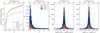 |
Fig. 1. Distances in the mass-radius plane between MaNGA galaxies and their assigned TNG galaxy pair. From left to right: cumulative percentage of galaxies at a distance given by Eq. (1). Histogram of distances with galaxies paired with three repetitions. Histograms of the differences in the mass and radius components in d. The majority of MaNGA galaxies are allocated a TNG pair that is within a relative difference of 25% in the mass-radius plane. |
In addition to analysing the distance distribution of the pairs, we compared the distribution in mass, size, and redshift of MaNGA galaxies to that of the matched sample. Because every TNG50 snapshot is associated with a redshift, the TNG50 galaxies in our sample have a discrete distribution of redshifts that reflects the 12 snapshots used for the match (see Fig. 2, right). Although the densest regions in the M − Re plane are comparable, some outliers cannot be matched in the TNG50 sample, for instance the large galaxies in the massive end, as seen in Fig. 2, left panel. In these regions of the plane repetitions are more frequent because TNG50 is a volume-limited sample. As the number of galaxies per mass decreases towards high masses, fewer massive galaxies are available. Another region where our sample appears to be less dense is at small Re; however, all MaNGA galaxies in this region are paired. The effect can then either be due to repetitions or to galaxies that are selected in multiple snapshots, but do not vary their properties across time. The mass distribution is properly reproduced.
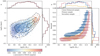 |
Fig. 2. Matched properties of the MaNGIA sample. Left panel: Distribution of mass and effective radius (M* − Re plane) of the TNG galaxies in the matched sample, colour-coded by redshift. The black contours indicate the density of galaxies in the MaNGA M* − Re plane. Right panel: Mass vs. redshift of the TNG galaxies in the matched sample. The colour-coding indicates the MaNGA subsamples: galaxies in the Primary sample in red, Secondary sample in blue, and Color-Enhanced sample in yellow. The contours show the distribution of the MaNGA galaxies in the plane. |
3. Construction of a mock dataset
Once the subset of TNG50 galaxies is selected (Sect. 2), a mock MaNGA-like datacube is constructed for each of the simulated galaxies in this sample. We describe the steps for generating mock datacubes below. We first define the FOV of the observations. This limits the particles and cells from the simulation that will contribute to form the spectra in the final datacube. Later, instrumental effects are included to emulate MaNGA observations. The procedure is based on Ibarra-Medel et al. (2019) and further details can be found there. A scheme of the steps followed is shown in Fig. 3.
 |
Fig. 3. Scheme followed to build a MaNGA-like datacube from a TNG50 simulated galaxy. Each step is described in Sect. 3 |
3.1. Field of view definition
The MaNGA survey uses IFUs formed by arrays of fibres distributed in a hexagonal pattern (Fig. 4). The bundles have five different sizes with diameters 12.5″, 17.5″, 22.5″, 27.5″, and 32.5″. These correspond to IFUs of 19, 37, 61, 91, and 127 fibres, respectively. To form a MaNGA datacube, the target is observed with one of these IFUs in three dithering positions resulting in a series of spectra associated with the fibre position in the FOV (Drory et al. 2015). Later, the fibre spectra are recombined and sampled onto a grid of 0.5 × 0.5 arcsec2.
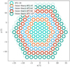 |
Fig. 4. Fiber arrays used by MaNGA. Outer fibres of each MaNGA IFU bundle are shown in a different colour and a thick line, while circles with a thinner line width show the other two dithers for the same IFU. Large bundles have the same fibre array than smaller bundles, with additional rings of fibres in the outer parts. The inner-most fibres (IFU-19, light green) are shared by all the bundle sizes. |
The survey is designed such that every galaxy has a similar spatial coverage. Each galaxy is allocated to the bundle size that optimizes either 1.5 or 2.5 Re coverage if they have been chosen for the Primary or the Secondary sample, respectively (Wake et al. 2017). Because the galaxies in our sample are matched in size and redshift, the proportion of galaxies assigned to each bundle is kept. However, to enable different sample selections, all mocks are produced with the largest bundle as smaller bundles can be obtained by removing the outer fibres.
The line of sight to the galaxy is defined by an unitary vector and the centre of the galaxy as listed in the TNG catalogue (SubhaloPos). For the galaxies that require up to three repetitions, we use the unitary vectors parallel to x, y, and z axes:  ,
,  , and
, and  for views 1, 2, and 3, respectively. When the TNG galaxy requires more than three repetitions, we define six isotropically distributed views. The orientation of the galaxy with respect to the observer is random as it is given by the position of the particles in the simulation cube (for more details, see Appendix B). The galaxy is observed from the distance defined by the redshift of the snapshot the galaxy was taken from.
We consider all the stellar particles and gas cells from the simulation collected by the Friends-Of-Friends (FOF, Turner & Gott 1976, Zeldovich et al. 1982, Huchra & Geller 1982) algorithm. The FOF algorithm groups particles together if they are within a given linking length of each other, or of another particle already linked to the group. In the TNG simulation, these groups trace the dark matter haloes. They may include more than one galaxy and, in this case, they are understood as a central galaxy and its satellites (Bose et al. 2019). This means that not only are the particles and cells to the target galaxy considered, but also those of the neighbouring galaxies, which reproduces a more realistic environment.
As the spatial axes of the cube are formed by the combination of multiple fibre observations, each fibre will have its own FOV. Atmospheric seeing is emulated by applying a random shift to the simulation’s particle positions. The shift follows a multivariate Gaussian distribution with FWHM = 1.43″. This shift is updated for each fibre and determines which particles fall in the FOV of the fibre.
3.2. From particles to light
The mock spectra are generated by including the stellar emission associated with the simulated stellar particles and the absorption produced by the presence of dust in the line of sight. Gas emission lines produced in HII regions are simulated by associating star-forming gas cells to CLOUDY templates (Ferland et al. 1998, 2017; see Appendix A3 in Ibarra-Medel et al. 2019 for implementation details3). However, because the interstellar medium model behind IllustrisTNG (Springel & Hernquist 2003) does not allow us to rely on the temperature and other thermo-dynamical properties of the star-forming gas, we remove the emission line contribution from the spectra for our analysis. As PYPIPE3D performs two spectral fits to extract emission lines before fitting the simple stellar population (SSP) template, the analysis of our spectra should be comparable to that performed on observations. Nonetheless, a non-perfect subtraction of the emission lines or the superposition of emission with absorption lines introduces an additional source of noise to the spectrum that could affect the template fitting. We evaluate this effect in Appendix C.
The SSP template was chosen with the following considerations. On the one hand, the SSP template used to create the mock cubes should be the same as the one used in the stellar population analysis (see Sect. 3.4) to avoid introducing uncertainties due to the assumptions behind the stellar populations template. On the other hand, to be consistent with the observations the stellar population analysis should be carried out with the same template used to process MaNGA observations. Therefore we adopt the SSP template used in Sánchez et al. (2022), MaStar_sLOG.
The MaStar_sLOG template consists of a set of synthetic spectra generated with the GALAXEV code (Bruzual & Charlot 2003, Yan & Wang 2010) based on MaNGA’s stellar library, MaStar (Yan et al. 2019). This library has spectra of a variety of single stars, in order to cover a wide range of effective temperature, surface gravity, metallicity and alpha-elements-to-iron ratio. GALAXEV combines these spectra assuming a Salpeter (1955) initial mass function (IMF) and PARSEC isochrones (Bressan et al. 2012) to produce synthetic stellar populations spectra. In particular, we use a subset of 273 synthetic spectra LSSP(λ, Z, t) comprising 39 ages between 0.0023 ≤ t≤ 13.5 Gyr with the sLOG sampling, seven metallicities 0.0001 ≤ Z ≤ 0.4 4 (see Camps-Fariña et al. 2022 for more details of the template age-metallicity sampling), and a linearly sampled wavelength range of 2000−10 000 Å at rest. Because the MaStar library was obtained using the same instrument as used for the MaNGA survey, the spectra have the same spectral resolution.
Because the datacubes are obtained imitating the IFU bundles, the spectra are constructed per fibre with the information of all the particles within the FOV of the fibre. Hereafter, we refer to these spectra as fibre spectra or Fi(λ), the i-th fibre spectrum in a bundle.
The ns stellar particles in the field of view of each fibre in the bundle contribute to form the spectrum. The j-th stellar particle is assigned the SSP with the nearest age and metallicity of the template. The spectrum is then mass-weighted and normalized by the mass-luminosity factor MLSSP associated with the corresponding SSP to obtain the flux. Next, the spectrum corresponding to the j-th stellar particle as a function of wavelength is given by
 (2)
(2)
where rj, Zj, tj, and mj are the distance, metallicity, age, and mass of the j-th stellar particle.
The presence of dust between the emitting source and the observer produces absorption in the optical range. As the simulation does not include dust particles, the dust content of the galaxies is estimated as a gas fraction following the recipe of Rémy-Ruyer et al. (2014), which is metallicity-dependent. The effect of dust is introduced in the mocks considering a simple screen model that attenuates the spectrum associated with every single stellar particle using the relation Aλ/AV from the Cardelli et al. (1989) extinction law with an extinction factor RV = 3.1. For this purpose, the extinction at Johnson’s V photometric band AV, j is calculated for the j-th stellar particle as the contribution of all the gas cells that are within the fibre’s FOV and placed between the observer and the stellar particle (see Ibarra-Medel et al. 2019). Specifically, the code considers the gas cells whose position (x,y,z) are in the FOV of the fibre. In the case that a section of a Voronoi gas cell is in the fibre FOV but its centre is not, the cell does not contribute to the extinction of the fibre spectrum. While this approximation may not be perfect, its impact is minimized by the fact that the large gas cells also imply low gas (dust) density; therefore, the underestimation of dust extinction due to these cells should be negligible. Then, the attenuated spectrum of the j-th stellar particle is
 (3)
(3)
The spectrum is then Doppler-shifted in wavelength according to the particle’s velocity in the line of sight vj and the redshift z at which the galaxy is placed. The spectrum of the i-th fibre is calculated as the sum of all the stellar contributions as
![Mathematical equation: $$ \begin{aligned} F_i(\lambda ) = \sum _{j}^{n_s} F_j^\mathrm{\,stellar\,\,obs}\left(\lambda + \lambda \times \left[\frac{v_j}{c}+z\right]\right) \,\,, \end{aligned} $$](/articles/aa/full_html/2023/05/aa45509-22/aa45509-22-eq7.gif) (4)
(4)
where c is the speed of light. Because the emission associated with each stellar particle is individually attenuated, we note that the dust extinction in different regions of a galaxy can be different.
To retrieve a rough value of the line of sight velocity, it is only necessary to have at least four particles in the FOV of the fibre to ensure a mean error of 50% ( , Wall & Jenkins 2012). However, more particles are needed to properly estimate the velocity dispersion. To study the kinematics of simulated galaxies, Walo-Martín et al. (2020) set a minimum number of nine particles per pixel to obtain a S/N = 3, assuming a Poisson distribution of the particles in the 2D projection of the galaxy. We calculate the percentage of fibres per galaxy that are under this value and find that only 30 galaxies in our sample have over 50% of their fibres under this threshold, indicating that this is not a dominant feature in our sample. Therefore, for the intrinsic maps we can ensure that almost all the galaxies have the minimum number of particles per fibre to recover the kinematics of the simulated galaxies. The fibres with fewer than nine particles in their FOV are mostly located at the outskirts of the galaxies, while all the fibres that cover the central regions of the galaxies have a good representation of the velocity dispersion. Additionally, the outskirt effects are minimized in the recovered maps due to the segmentation scheme of PYPIPE3D as the spectral fitting code recombines the spaxels to achieve a target S/N. Therefore, the kinematics at the galaxies’ outskirts are calculated from a combination of spaxels (which are also a combination of individual fibre spectra), providing a better statistic for the kinematic extraction.
Even though the dust model used in this work is rather simple, it is not less complex than the reverse analysis that PYPIPE3D performs. While the dust modelling in the two cases is similar, recovering the extinction during the spectral analysis is not as trivial a task as simply inverting the problem. This is because the attenuation effect is implemented per stellar particle spectrum before shifting and integrating the contribution of all the stellar particles in the fibre during the mocking process, while PYPIPE3D recovers one extinction value per observed spectrum. Another layer of complexity in the inversion problem is that the spectral fitting code is limited to derive properties from the observable light, and therefore cannot retrieve the information of the obscured light beyond the optical depth (see Sect. 4.2). Other more complex approaches to model dust extinction include radiative transfer (SKIRT, Baes et al. 2011, Baes & Camps 2015, or SUNRISE, Jonsson 2006, Jonsson et al. 2010), where the gas cells are treated as a Voronoi grid, which is compatible with how the simulation is computed. These approaches are considerably more expensive computationally than ours.
At this point the fibre spectra are saved in the row-stacked spectra (RSS) format. For control, the intrinsic properties of the stellar particles in the FOV of the fibres are saved as an extension of the RSS file. The luminosity-weighted (LW) values of age and metallicity, are computed using the MaStar_sLOG and weighting by the flux at 5000 Å. To be consistent with the stellar analysis applied to the datacubes, these are added in log-scale for the i-th fibre as
 (5)
(5)
While the age t, the metallicity Z, and the mass m of the particles cover continuous ranges, the luminosity weights w depend on the template’s MLSSP which has a discrete sampling in age and metallicity.
Because the particles get assigned a spectrum from the template, the fibre spectrum is formed by a combination of discrete ages and metallicities. To analyse how the intrisic ages and metallicities are affected by this discretizing step, an additional set of control properties is generated. These are calculated as in Eq. (5), but replacing the ages and metallicities by the assigned values of the SSP template.
3.3. Building MaNGA-like datacubes
To realistically emulate MaNGA observations, we include a series of instrumental effects that are detailed in this section. We first reproduce the fibre bundle dithering scheme (Sect. 3.1) to obtain the spatial sampling and resolution of MaNGA. The spectrum corresponding to each fibre is constructed as in the previous section (Sect. 3.2). Noise is added to the spectra. Finally, the fibre spectra are re-sampled to MaNGA’s spatial grid format.
The spectra observed in MaNGA are affected by noise introduced by the detector, of a Poisson distribution nature. Because the spectra are sky-subtracted to the Poisson-limit level, the noise is ideally distributed following a Gaussian distribution (Law et al. 2016). We follow the recipe of Ibarra-Medel et al. (2019) to emulate BOSS spectrograph noise which mimics the detector’s behaviour by increasing the noise towards the edges of the wavelength range, with a plateau value F0. As MaNGA observations target a signal-to-noise ratio (S/N) of 5–10 at the outskirts of the galaxies (at 1 − 2Re; Bundy et al. 2015), we fix F0 to obtain a S/N ∼ 5 in the r-band at 2 Re. Because the noise is added to the fibre spectra before computing the spatial grid, the value of F0 is estimated from the hexagonal ring of fibres with radius closest to 2 Re (see Fig. 4). This produces a wider variety of S/N values in the mocks, which is more similar to observations.
The stacked spectra corresponding to each galaxy are then used to reconstruct the spectral cube. MaNGA’s spatial grid is formed by 0.5 × 0.5 arcsec2 pixels. The contribution of a fibre to the pixels in the grid is weighted by the distance rp, i of the pixel p to the centre of the fibre i. If rp, i > 1.6″ the contribution of the fibre to the pixel is zero. Otherwise, the weights are defined as
 (6)
(6)
where σrec = 0.7″ (Law et al. 2016) and ωT is a normalizing factor to keep the total flux constant.
The mock datacubes have the format detailed in Sánchez et al. (2022) to be analysed by PYPIPE3D (Lacerda et al. 2022), namely a FITS file comprising three extensions: the flux datacube in units of 10−16 erg s−1 Å cm−2 per spaxel, a second datacube with the flux error, and a final extension comprising a datacube with a mask for bad pixels, all with a linear fixed step in wavelength.
The intrinsic and assigned values of the galaxies that were saved per fibre for control (Sect. 3.2) are now spatially recombined in the same way as the mock datacubes. This results in a set of 2D maps with the instrinsic and assigned stellar properties of the simulated galaxies with the same spatial resolution as the datacubes. We refer to the maps generated from the continuous properties of the galaxies as the intrinsic maps, while those formed with the discrete ages and metallicities from the template are the assigned maps.
3.4. From spectra to stellar population maps
The post-processing of the mock datacubes is performed with PYPIPE3D (Lacerda et al. 2022), the PYTHON implementation of the PIPE3D code (Sánchez et al. 2016a,b). The goal of this programme is to disentangle the contributions to the emission produced by the different stellar populations and extract the emission line information from galaxy spectra.
For this purpose, it is necessary to separate the kinematic and dust extinction effects in the observed spectra and remove emission lines before finding the best-fitting SSPs. Therefore, the first step this software performs on given galaxy spectra is a non-linear fit to determine the extinction ( ) and the stellar kinematic (σ* and z) parameters. A parametric fit is then used to approximate strong emission lines. Once the emission line contribution is calculated, it is subtracted from the original spectra to perform the stellar population linear fit.
The SSP fit consists in finding the best-fitting linear combination of SSP spectra (positive contributions only). As the spectra generally have lower S/N towards the edges, a binning scheme is necessary to extract the SSP information from these regions. In particular, PIPE3D uses a Continuous plus S/N binning algorithm to define how adjacent bins are going to be co-added. As this scheme sets a goal S/N at the same time as it requires continuity in the surface brightness, the shape of the resulting spatial bins follows the isophotes, which typically have an arc shape rather than the square or round bins formed with the Voronoi binning scheme. The S/N is set to 50, although the final S/N value per bin is generally lower because of the brightness restriction of the algorithm (see Sánchez et al. 2016b).
Once the stellar spectra have been decomposed into a set of SSPs, the code saves the spatially resolved star formation histories of the galaxy, as well as its maps of stellar age, metallicities, and kinematics (see Fig. 5, recovered maps on the right-hand side). Other outputs of the PYPIPE3D analysis include the emission line properties and stellar absorption indices.
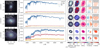 |
Fig. 5. Three simulated galaxies with stellar masses 109 M⊙, 1010 M⊙, and 1011 M⊙ show the mocking process. Panels on the left-hand side show the stellar mass density of the galaxies, while the central panels show their spectra at different radii (centre in blue, 0.5Re in red, and 1Re in yellow). Squared panels on the right-hand side show the stellar properties derived directly from the particles (top row for each galaxy) and recovered from the spectral cubes with PYPIPE3D (bottom row for each galaxy). From left to right, these panels show the V-band reconstructed image (mass density for the particle maps), luminosity-weighted age, luminosity-weighted metallicity, LsOS velocity, and velocity dispersion. As galaxy mass increases, the spectra are redder. Stellar maps are, in general, properly recovered. |
4. Results
We evaluate the performance of the complete pipeline by comparing the stellar population and kinematic maps produced during the mocking process (TNG50 intrinsic, assigned, and recovered maps; see Table 2), and then compare the simulated sample with the observed one (TNG50-recovered and MaNGA-recovered, see Table 2). While the maps of the simulated galaxies were obtained as described in Sect. 3, those of the observed galaxies correspond to the latest PYPIPE3D analysis release for 10 000 MaNGA galaxies5 (Sánchez et al. 2022). In both cases the fitting code and the SSP template used for the analysis are the same. The maps considered in this work are the V-band reconstructed image, the luminosity-weighted age and metallicity, LOS velocity, and dispersion. First, we study the effect of discretizing in age and metallicity when associating stellar particles to a spectrum in the MaStar_sLOG template. Second, we analyse how well the parameters of the simulated galaxies are recovered from the spectral fitting by comparing them with a set of analogous stellar population maps calculated directly from the particle information of each simulated galaxy (assigned maps). Third, we compare the SSP maps derived from our mock datacubes with those derived from MaNGA observations.
Simulated and observed datasets used for comparison.
For this section, all the stellar population maps have been masked when the median intensity had S/N < 3. Because the mock datacubes were produced with the largest IFU bundle of 127 fibres, an additional mask was applied when their corresponding IFU bundle size is smaller (see Sect. 3.1). In this case, the allocated IFU size was the same as its observed counterpart.
4.1. Discretization effect in age and metallicity
The simulations produce stellar particles with ages and metallicities that span continuous ranges (constrained only by numerical limits). When the mock datacubes are produced, the particles are assigned to a limited number of SSPs (273) with discrete distributions in age and metallicity. The way the SSP grid is defined will determine how well the continuous values are represented by the template.
We compare the intrinsic LW age and metallicity of the simulated galaxies before and after being assigned an SSP from the template. For this we calculate the mean LW age and metallicity within 1Re from the intrinsic and the assigned LW age–metallicity maps per simulated galaxy. The difference between these values is shown in Fig. 6 (assigned minus intrinsic in log-scale). The age differences spread around zero, with a larger scatter towards young ages (ages < 5 Gyr). The mean of all differences is Δlog(AgeRe) < 0.003 dex, which is smaller than the standard deviation of 0.004 dex.
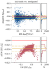 |
Fig. 6. Difference between the intrinsic and assigned mean LW-age and metallicity (top and bottom, respectively, both in log-scale) within 1Re per galaxy (dots), calculated from the respective 2D maps. The yellow solid and dashed lines indicate mean and standard deviation of the differences of the complete set of galaxies. While ages are slightly younger after being assigned, metallicities show a greater negative deviation from the intrinsic values. |
After assignation, the LW metallicity is systematically lower than the intrinsic value. Furthermore, the assigned values tend to deviate more from the intrinsic values at low ([Z/Z⊙]< − 0.3) and high ([Z/Z⊙]> 0) metallicities, reaching maximimum differences of ∼0.1 dex. The greater deviation towards high metallicities could be related to TNG50 galaxies generally having particles with metallicities greater than the template’s highest value ([Z/Z⊙]> 0.372), being more frequent at higher masses (see Appendix D). These particles’ metallicities are underestimated when discretized, resulting on an average lower metallicity of the galaxy. Within the range where the particles’ metallicity overlaps with the template’s range of metallicity, the discretization could still produce, on average, differences with the intrinsic values. This could occur because the intrinsic value distributions of the simulated galaxies may not be well represented by the sampling of the template or because the interpolation method should be revised.
4.2. Recovering physical properties with PYPIPE3D
Determining age, metallicity, and extinction from a spectrum is a highly degenerate problem. Even in the most favourable case where the input spectrum is a linear combination of spectra from the SSP template, recovering ages and metallicities through template fitting is a challenging task. Therefore, to see how well these properties are disentangled by PYPIPE3D, we compare the stellar population maps recovered with PYPIPE3D (recovered) with a set of maps that were produced directly from the stellar particle properties after being assigned the nearest ages and metallicities from the template’s discrete grid (assigned maps, see Sect. 3.2). The latter maps are produced with the same spatial properties as the mock datacubes so that the resolution is comparable. Additionally, the age and metallicity maps are luminosity-weighted and averaged in log-scale, like those recovered by PYPIPE3D.
Qualitatively, except for differences due to the binning in the recovered maps, we find that the spatially resolved properties are properly recovered, as seen in the examples in Fig. 5 (right panels). As the degeneracy in the determination of ages and metallicities is case-sensitive, it is worth analysing how the age and metallicity estimations depend on the galaxy properties. We calculate the difference between the average values within 1 Re of the recovered and assigned maps for each galaxy (age and metallicity in log-scale). In Fig. 7 we see that the estimated values of extinction tend to be lower than the real ones as their values grow (bottom right panel). This is a well-known problem of any inversion fitting code: the code can only measure the stellar properties of the observed light within the optical depth, and cannot recover the information of the obscured light beyond it. Therefore, the derivation of the recovered extinction is limited to the observable light, while the intrinsic extinction is estimated from all the particles along the line of sight assuming an ideal and completely transparent galaxy. This produces a systematic underestimation of the recovered extinction as the intrinsic extinction grows (see Fig. 12 in Ibarra-Medel et al. 2019, and Fig. 7 bottom right panel in this work). Although this means that the recovered spectra are redder than the original ones, this is not evidently compensated by an older or metal-rich estimation. There is, however, a degeneracy between age and metallicity. The ages estimated from the recovered data tend to be systematically lower than those of the assigned maps (−0.05 dex on average) and the metallicities tend to be estimated with higher values (+0.05 dex on average). This effect is more notorious towards low metallicities, where the differences in ages and metallicity are around 0.1 dex. Although we find systematics in the recovered ages and metallicities, we note that the deviation from the assigned values is within the expected range of 0.1 dex (Cid Fernandes et al. 2013, 2014, Sánchez et al. 2016b, Lacerda et al. 2022) and within 2σ on average (within 1σ for extinction).
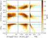 |
Fig. 7. Differences in age, metallicity, and extinction recovered by PYPIPE3D. The difference Δ is calculated as recovered-assigned for age and metallicity [dex] and as recovered-intrinsic for Av. The panels show the number density of galaxies of the differences across each parameter. The solid and dashed cyan lines show the mean and standard deviation of the differences, respectively, while the dashed magenta lines show 2σ deviations from the mean. An age-metallicity degeneracy is seen as PYPIPE3D tends to recover systematically younger ages and higher metallicities than expected. However, the recovered values are within the expected errors of 0.1 dex. As expected, extinction is increasingly underestimated as its value grows. |
After the full mocking process, the velocity dispersion of the galaxies is, on average, lower compared to the intrinsic values (Fig. 8, left panel). However, this effect is small given that the mean decrease is ≲0.1 dex, which is still within 1σ. To analyse if the reddening effects of redshift and extinction are properly disentangled, the right-hand side of Fig. 8 shows the difference between the intrinsic and recovered extinction as a function of redshift. The recovered extinction values are lower than the intrinsic values mostly at the lower redshifts (z < 0.06). This is likely related to the sample of galaxies considered, as it has a greater proportion of massive galaxies at higher redshift, which are likely to have a low gas mass fraction, and therefore less dust than those selected at low redshifts. Furthermore, a degeneracy between redshift and extinction should produce the inverse effect.
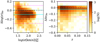 |
Fig. 8. Left panel: differences between intrinsic and recovered velocity dispersions as Fig. 7. Right hand-side panel: differences in extinction as a function of redshift. |
4.3. Comparing simulations to observations
We now compare the recovered SSP maps of simulated galaxies with their observed counterparts. Given the size of the sample, a detailed analysis cannot be done for all the galaxies. Therefore, we compare the integrated properties of the whole sample in the following subsections.
4.3.1. Individual stellar maps
To assess how well the mocks reproduce the observational features in the data, we show the stellar population and kinematic maps obtained for ten example galaxies compared with their MaNGA-observed counterparts (Fig. 9). These galaxies were chosen to represent ten regions of the M* − Re plane. For this purpose, we defined five mass bins (separated by the following mass limits:109.5, 1010, 1010.5, and 1011 M⊙) and subdivided each bin into two sizes (first and last 50th percentile in Re [kpc] within the bin). We then choose the galaxies with the most similar mass and size to the median values in each of the ten bins. Because there are two galaxy sizes for the same mass, we refer to the galaxies with larger Re as extended and the smaller Re as compact.
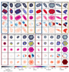 |
Fig. 9. Simulated and observed recovered maps. The left panels show ten TNG50 recovered stellar population and kinematic maps. From top to bottom in each subpanel: the V-band reconstructed image, LW-age, LW-metallicity, LOS velocity, and velocity dispersion maps. The right panels show the MaNGA counterparts of each of the galaxies in the left panels. These examples were chosen to represent ten regions of the M* − Re: five mass bins (delimited by 109.25, 109.75, 1010.25, and 1010.75 M⊙), which correspond to the columns, with increasing mass from left to right, and two Re[kpc] regions per mass bin (rows, increasing size from bottom to top). |
Mocks realistically reproduce the observational and pipeline effects seen in the observations including spatial resolution and binning. The noise level is adequate to recover a segmentation that is comparable to observations, as determined by the S/N < 3 clipping in both cases (Fig. 9).
While only ten example galaxies per mock–observed sample are shown in Fig. 9, these were chosen to have representative masses and sizes of different regions of the M* − Re plane. We see that the galaxies are older, more metal-rich, and exhibit less rotation as they are more compact and massive. The extended simulated low- and intermediate-mass examples have a distinctive central component and show negative gradients in age and metallicity, while the observed counterparts show flatter distributions and a more prominent disc component. At high mass, the compact simulated examples are fast-rotating, while the observed galaxies have higher velocity dispersion and disrupted LOS-velocity maps, corresponding to a typical slow-rotating galaxy (bottom) and an interaction with a nearby galaxy (top).
4.3.2. Integrated properties
To compare the global properties of the observed sample with those of the mocked sample, we analyse how the mean values of age, metallicity, LOS maximum velocity, projected V/σ, and dispersion distribute across the M* − Re plane. All values are calculated within 1 Re. While the projected V/σ is calculated as in Cappellari et al. (2007), the values obtained can differ from other works since this parameter is sensitive to the definition of the reference systemic velocity of the galaxy and the spaxel binning, which in our case is CS-binning instead of Voronoi. However, the values shown in Fig. 10 are directly comparable as they were calculated in a consistent manner for the observed and simulated galaxies.
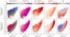 |
Fig. 10. TNG50 galaxies in the M* − Re plane (top) and their MaNGA counterparts (bottom). The galaxies are colour-coded from left to right by their mean LW-age, LW-metallicity, LOS maximum velocity, dispersion, and projected V/σ calculated within 1 Re from the recovered maps. The trends seen in the observed sample are replicated in the simulated sample with a greater dependence with galaxy size rather than mass. Although there is a discrepancy between the maximum values in dispersion and minimum values in age, the galaxies with these values lie in analogous regions of the plane. |
For the observed sample, older and more metal-rich galaxies lie on the lower and more massive side of the plane, as seen in Fig. 10 (top panels). These main trends are replicated in the matched TNG50 sample (bottom panels). However, the age, metallicity, and V/σ of the simulated sample have a stronger dependency on the size of the galaxy than those of the observed sample, which show a clearer correlation with stellar mass. In contrast, the LOS maximum velocity is strongly correlated with stellar mass in the simulations, with the highest values at the most massive end. This is consistent with the lack of simulated galaxies with low V/σ in this region, while the lack of galaxies with high V/σ at low masses could be due to slightly higher values of dispersion than in observations.
As expected, higher velocity dispersion values are found at the most massive end. However, the highest velocity dispersion of the simulated galaxies is limited to ≲150 km s−1, while observed galaxies reach values of 250 km s−1. Similarly, the youngest galaxies of both samples lie in the low- to intermediate-mass and most extended regions of the M* − Re plane, but here the most frequent age for the simulated galaxies is around 2 Gyr, while for the MaNGA galaxies this value is 1 Gyr younger.
4.3.3. Gradients
To analyse how the age and metallicity of the observed sample and the mock counterpart vary across the galaxies, we consider the mean values of the LW-maps in three annuli: within 0.5 Re, between 0.5 Re and 1 Re, and from 1Re to 1.5 Re. Then we calculate the median values per mass bin for both samples.
The best match in age between observations and mocks is found within 0.5 Re for high-mass galaxies (1010.5 M⊙< ), even though for lower-mass galaxies the discrepancy is 1 Gyr (top row in Fig. 11). Towards the outer regions of the galaxies, the discrepancy between observed and mocked increases. The mocks have a flatter distribution of ages across mass outside 0.5 Re, while the observed galaxies have a steep increase in ages with mass.
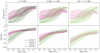 |
Fig. 11. Median luminosity-weighted age (top panels) and metallicity (bottom panels) per mass bin at increasing radii for MaNGA galaxies (green) and TNG50 fully mocked with PYPIPE3D (solid magenta line). The median values for the TNG50 intrinsic and assigned maps are shown with dashed and dot-dashed lines to compare the median shift produced by the mocking process. The shaded areas span from the 20th to the 80th percentile. |
The best match in metallicity between mocks and observations is found in the outer regions, in contrast to what is seen for age. Compared to the observations, the simulations form more metal-rich bulges in low- to intermediate-mass galaxies.
As seen before, there is some degeneracy when recovering age and metallicity with PYPIPE3D; however, the discrepancy between observations and simulations is still evident when we compare these values with those obtained from the particle maps (dashed lines in Fig. 11). As pointed out in the previous section, PYPIPE3D tends to predict lower ages than the real ones. This effect is greater in the outer regions of the galaxies, suggesting that the code’s performance might be affected by low S/N.
5. Reliability of the sample and caveats
The trends of the observed physical properties are recovered in our sample, although there is still a mismatch between the samples. We discuss here how the assumptions made when creating the mock datacubes could be the source of this discrepancy.
5.1. Simulations
The mock galaxies are older than those observed for MaNGA in the low- to intermediate-mass regime. This behaviour has been observed by Nelson et al. (2018) for TNG100 galaxies. The results between that work and ours might originate in the different samples of galaxies used in each case and/or a resolution difference since the cosmological volumes of the TNG50 and TNG100 simulations differ.
In the simulated sample the compact galaxies have old ages (> 5 Gyr) and high metallicities ([Z/Z⊙]> 0) at low masses, which is not seen in the MaNGA sample. In contrast to more extended galaxies in the same mass regime, the simulated compact galaxies are old, and therefore their age estimates should not be affected by strong emission lines. The difference between observed and simulated galaxies in this particular region of the M* − Re plane could be related to the larger fraction of satellite galaxies in MaNGIA (55%) compared to MaNGA (25%, based on the Yang et al. 2007 group catalogue). To analyse the effect in satellite and central galaxies of the observed and simulated samples, we compute the median LW-ages and metallicities per mass bin as in Sect. 4.3.3 (age and metallicity per galaxy is calculated as the mean value within 1Re from the recovered maps), now separating satellites from centrals. We consider a galaxy as ‘central’ if it is not a satellite. The satellite galaxies are, on average, older and more metal-rich than central galaxies (see Fig. 12), both in the observed and simulated sample. Older ages seen for satellite galaxies are consistent with a gas stripping scenario (Gunn et al. 1972, Quilis et al. 2000), where a more massive nearby galaxy removes gas from the less massive satellite limiting its ability to form new stars. While central galaxies may accrete stars and gas with low metallicities resulting in an effective lower metallicity, the enhanced metallicity observed in satellite galaxies might be connected to ‘strangulation’ processes, which operate more effectively in the low- to intermediate-mass regimes (M* < 1010 M⊙; Peng et al. 2015).
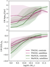 |
Fig. 12. As in Fig. 11, but taking the mean age and metallicity per galaxy up to 1Re. The solid and dashed lines represent the median age (top panel) and metallicity (bottom panel) per stellar mass bin of the central and satellite galaxies, respectively. TNG50 galaxies are plotted in magenta, while MaNGA galaxies are plotted in green. |
While the central and satellite galaxies have consistent behaviours in both observed and simulated sample when considered separately, there is still a discrepancy between the satellite and central simulated and observed galaxies. The simulated galaxies with stellar masses lower than 1010.5 M⊙ are older and more metal-rich than those observed, while at higher masses we find the inverse behaviour. The age discrepancy at low and intermediate masses can also be related to a selection bias in the observations. While MaNGA targets are selected based on their Mi, brighter galaxies are more likely to be observed. Therefore, at a fix mass, MaNGA may have a larger fraction of younger galaxies than the simulated sample simply because the larger proportion of recently formed hot stars makes these galaxies easier to detect.
In the high-mass regime the simulated galaxies show considerable rotation (V/σ > 1, right top panel in Fig. 10), which contrasts with the typically slow rotation in the observed galaxies. The behaviour of the massive simulated galaxies is compatible with the overpopulation of red spirals and late-type galaxies at high masses reported in Rodriguez-Gomez et al. (2019) and Huertas-Company et al. (2019), respectively. As these results were found for the TNG100 simulation, a different behaviour could be expected for TNG50. However, Donnari et al. (2021) show that TNG50 has a lower quenched fraction of galaxies at high masses than other TNG simulations (TNG100, TNG300), suggesting that the behaviour is still present in the highest resolution volume.
5.2. Stellar population templates
The determination of ages and metallicities from spectra relies heavily on the SSP template, which depends on the IMF, isochrones, and stellar library assumed to build the template, and on the sampling in age and metallicity of the template. The impact of the template choice in this work can be separated into two aspects. On the one hand, the generated spectra and the recovered maps of the mocks depend on these choices. On the other hand, observed galaxies do not necessarily behave as the models do.
By selecting the same template to produce the mocks as to analyse the observed datacubes, the uncertainty introduced by the assumptions is minimized when recovering the stellar population properties of the simulated galaxies. In terms of age and metallicity estimations from the mock data, the most relevant effect of the template choice is in the luminosity-weighted maps as age and metallicity, since the M/L ratio is given by the template. It is worth noting that the IMF assumed in the template used in our mocks is different to that used in the TNG simulation. However, as in Nanni et al. (2022a), this should not introduce large inconsistencies as a universal IMF is assumed in the simulations and in the templates.
For comparison, we produce a reduced sample of 100 mock assigned LW-maps using the Maraston et al. (2020) template (MaStar_MA19 from now on) and compare these maps with the assigned maps produced with the MaStar_sLOG template, for the same 100 galaxies. The MaStar_MA19 template is based on MASTAR, the same stellar library as used in this work. It combines Cassisi et al. (1997) and Schaller et al. (1992) isochrones, and it assumes a Kroupa (2002) IMF. This IMF’s positive slope for low masses (< M⊙) and higher fraction of massive stars than the Salpeter IMF is more similar to the Chabrier (2003) IMF, the one used in the TNG50 simulations. The difference between the two templates in LW-metallicity is negligible (Δ[Z/Z⊙]< 0.03), and the difference in LW-age is only evident for young galaxies. These differences are smaller than the uncertainties of the parameter estimation during the post-processing of the datacubes, as shown in Fig. 13. Although the MaStar_MA19 template is based in the same stellar library as used in our work (Sect. 3.2), the differences observed can also be affected by the different sampling in age and metallicity in each template. Although this highlights the complexity in the age determination through SSP template fit, it also shows that the assumptions behind the different templates have a limited impact in the LW-ages and metallicities when generating the mocks.
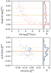 |
Fig. 13. Difference in the LW-age (top) and metallicity (bottom) obtained with MaStar_MA19 and MaStar_sLOG templates. The properties were calculated as the mean values within 1 Re from the assigned maps. While the metallicities are comparable, the assigned ages tend to be older when using the MaStar_MA19 template. |
The age and metallicity sampling of the SSP template plays a role both when producing the mocks and in the retrieval of the stellar parameters with the spectral fit. Here we focus on the first effect. As seen in Sect. 4.1, the sampling of the SSP produces a systematic shift in the average metallicity of galaxies, where intrinsic values are more metal-rich than those assigned (Fig. 11, bottom row). On the one hand, this behaviour could be related to the metallicity range covered by the SSP template, as some stellar particles in TNG have metallicities that exceed the highest value in the template (Z = 0.4, see Appendix D). On the other hand, the spacing of the metallicity template and/or the interpolation method used to assign an SSP spectrum to a stellar particle (nearest interpolation) may not properly represent the intrinsic properties of the particles, resulting in lower metallicities than expected.
Finally, the stellar population maps retrieved from the mock spectra are also affected by the internal degeneracy of the SSP template since different combinations of spectra from the template could result in a similar added spectrum. This leads to age and metallicity estimates that deviate from the real ones. While age and metallicity estimates from real spectra are also affected by this, the effect can be quantified with the mocks because they were built as a linear combination of the spectra in the template. If there is no degeneracy, the combination of spectra should be perfectly retrieved.
Recovering ages and metallicities from mocks produced with the same SSP template as used in post-processing is an idealized scenario where the nature of the galaxies is fully known. While the uncertainty is minimized by choosing the same SSP to generate the mocks, the assumptions may not be identically valid for real galaxies. As the degeneracy when recovering ages and metallicities through template fitting is non-negligible, this can lead to discrepancies between the samples. This could occur in particular for young stellar populations where the variations in the spectra are more significant.
We note that these properties in the mock sample recover the overall trends seen in the observed sample. This is in spite of the complexity of age and metallicity determination with SSP fits for real spectra, and the fact that the simulated sample was not built to match MaNGA’s age and metallicity distribution.
5.3. Emission lines
While interesting information is contained in emission lines, they are difficult to simulate reliably. Because studying galaxy line emission is not the final scope of this work, we produce spectra without it. Nonetheless, this choice motivates a further study of the effect of emission lines on the stellar population analysis. In Appendix C we show that strong emission lines can lead to lower estimates of metallicity and age. Although a detailed quantification of this effect is beyond the scope of this work, we find that it can be more important than the uncertainty in the retrieval of ages and metallicities when only considering the stellar component.
In our sample this means that the match with observations in metallicity and age could be slightly improved by adding emission lines as the discrepancy is stronger where the youngest galaxies lie (extended low- to intermediate-mass region in the M* − Re). These galaxies tend to be star forming as they exhibit such young ages. Therefore, they should still have massive stars capable of ionizing the surrounding gas and producing emission lines.
5.4. Comparison with other works
Our work is the first to construct MaNGA-like mock datacubes of simulated galaxies from TNG50 that match the number and mass-size-redshift distribution of the observed MaNGA galaxy sample. This allows us to make extensive comparisons between simulated and observed galaxies connecting the observed properties of current-epoch galaxies to their formation and evolutionary history. Previous studies have only matched smaller subsamples of simulated galaxies to MaNGA observations. We discuss here the similarities and differences between the various approaches. We consider the works by Ibarra-Medel et al. (2019, hereafter I–M), Nevin et al. (2021, N21), Bottrell & Hani (2022, B&H), and the series Nanni et al. (2022a, N22a) and Nanni et al. (2022b, N22b). For a fast comparison, the characteristics of each of these works are condensed in Table 3.
Comparison with similar works.
The N21 and I–M approaches are based on numerical hydro-dynamical simulations of single galaxies or pairs of merging galaxies. Because our goal is to generate a sample of galaxies that is statistically comparable to the MaNGA survey, a large enough sample is needed to cover a variety of galaxy types. In this sense, hydro-cosmological simulations are ideal as they produce a range of different galaxies in a realistic environment. Additionally, high resolution is required to capture the structures that can be resolved by MaNGA. We therefore use TNG50 simulations. The common choice with other works (B&H, N22a, and N22b) stems from TNG50’s good compromise between resolution, number of available galaxies and the fact that they are immersed in a cosmological context.
To construct the spectra, we employ a simpler approach than N21 and N22a, who run the radiative transfer (RT) codes SUNRISE (Jonsson 2006, Jonsson et al. 2010) and SKIRT (Baes et al. 2011, Baes & Camps 2015), respectively. Our spectra are the result of linearly combining the individual mass-weighted and doppler-shifted SSP spectra associated with each stellar particle, considering a simple dust screen model. RT codes use Monte Carlo methods to emulate the physical processes associated with dust (scattering, absorption, and emission) in the LOS of light-emitting sources. These codes perform a more complex treatment of dust as they consider a localized dust contribution and have been used to produce mock galaxy imaging (Rodriguez-Gomez et al. 2019, Torrey et al. 2015). However, as computation time scales with wavelength sampling, they are computationally very expensive when the aim is to produce high-resolution spectra (Rλ > 2000). To speed up this process, N22a compute the dust extinction at low spectral resolution. Furthermore, Zanisi et al. (2021) argue that dust modelled by SKIRT does not necessarily produce more realistic mocks as extinction modelling is not a trivial task that depends on several choices that could modify the outcome (i.e. estimation of dust from gas in the simulations, geometry assumed). They use a convolutional neural network framework to compare how TNG simulated galaxies reproduce observed morphologies using mock images produced with SKIRT (as Rodriguez-Gomez et al. 2019). Their framework recovers a higher agreement between the mock photometric images and the observed ones when the dust effect is removed from the synthetic images than when it is included (see Sect. 8.3 in Zanisi et al. 2021). For these reasons, we stick to a simpler approach to dust emission that is less computationally demanding. However, because the modelling of the dust in our mocks is similar to the inverse analysis carried out by PYPIPE3D, the performance of the code might be biased to more accurate results than in real observations where the nature of the extinction is not fully known.
To build IFU datacubes, a complex pipeline is needed. While this work, B&H, and I–M reproduce MaNGA fibre observations to form the spatial grid of the datacubes, N21 and N22a mimic this effect by convolving a high-resolution datacube with a comparable PSF in the spatial axes. By generating the fibre spectra, the spatially correlated noise of the datacubes is reproduced, as the noise is introduced by the spectrograph’s detector and propagated to the datacubes during the recombination of the fibres. While it is possible to combine the output of an RT code with the REALSIM code used by B&H to fully imitate MaNGA’s pipeline, our approach (and I–M’s) is considerably less time-consuming because the spectra are built per fibre, which translates to building up to 381 spectra per datacube (the largest IFU has 127 and three dithering positions) instead of producing a factor of ten more spectra to form the spatial grid that covers the IFU’s FOV with MaNGA’s spatial sampling (70 × 70 pixels of 0.5 × 0.5 arcsec2).
The stellar population templates used in each case are different as they either use different stellar libraries or assume different stellar formation models (e.g. IMF, isochrones; see references in Table 3). As in our work, the approaches of I–M and N22a are intended to perform a stellar population analysis on the mock datacubes. Therefore, the SSP templates of choice are the same as those used to process the MaNGA observations with the different stellar population analysis pipelines. This work and N22a, N22b use SSPs based on the MaStar library.
The spectral fitting code used in N21, N22a, and N22b is ppxf (Cappellari & Emsellem 2004, Cappellari 2016), which groups the spaxels in Voronoi bins (Voronoi 1908a,b) to achieve a minimal S/N per bin defined by the user. In contrast, the binning scheme used in the fitting codes PIPE3D and PYPIPE3D (used in I–M and this work, respectively) is CS-binning, which produces bins that not only target a minimal S/N, but also minimize the flux variation within the bin (Sánchez et al. 2016b). Therefore, the shapes of the CS-bins align with the galaxy’s isophotes.
In N22a and I–M only emission lines due to star-burst regions are simulated. While N22a associate stellar particles younger than 4 Myr with the MAPPINGSIII template (Groves 2004), I–M model emission lines assume that the star-forming gas forms young stars with ages 2.6 Myr. Their emission spectral template was produced with the CLOUDY code (Ferland et al. 1998). Although we do not include emission lines for the spectral fitting step, the emission lines are calculated as in I–M and are saved in an extension of the datacube file. In addition to the uncertainties of the modelling of these features, the emission lines have not been flux-calibrated. While other approaches use Mappings III, a specific young stellar populations template that includes emission lines associated with young stars, we adopt the same stellar template used for the SSP post-processing for the complete age range to avoid introducing further uncertainties in the SSP fit.
N21 includes emission not only from starburst regions and stars, but also from AGN activity. To do this, AGN spectral energy distributions (SEDs) are included by associating the black hole accretion rates derived from the simulations to the SED template from Hopkins et al. (2006).
N21 find that kinematic maps can change significantly after emulating the whole mocking procedure by increasing the velocity dispersion measurement. This effect is boosted when including dust scattering and absorption in the SUNRISE prescription. They find that the presence and treatment of AGN could also have an effect on the kinematic estimates. We do not report an increase in velocity dispersion after mocking.
6. Conclusions
We present a catalogue of 104 TNG50 galaxies, called MaNGIA, that matches MaNGA’s target selection, while maximizing the selection of unique simulated galaxies. MaNGA-like datacubes were generated for each of the galaxies in the catalogue and these were post-processed to obtain stellar population and kinematic maps that are comparable to those in Sánchez et al. (2022). MaNGIA is the first sample of 10 000 fully mocked and post-processed datacubes that mimic MaNGA’s target selection. This sample not only reproduces the global physical properties of the observed galaxies, but it also emulates observational effects to produce realistic stellar population and kinematic maps. Because these maps were generated with the same pipeline, they are directly comparable with observations.
This sample is ideal to connect the galaxies’ observable properties with the physical processes occurring within them, as many of the latter cannot be directly observed (i.e. accretion history, black hole growth), but can be easily extracted from the simulations. Therefore, this dataset can be used to constrain the cause of observables and infer the history of the observed galaxies.
The sample is also well suited for machine learning applications given its large volume and realistic observational features. The sample, mock datacubes, and derived maps are made publicly available with the publication of this paper.
While only stellar mass, size, and redshift were matched, the overall trends in age, metallicity, and velocity dispersion are in good agreement with observations. The sample was obtained with a one-to-one match to MaNGA galaxies, but the dataset presented in this work is intended to be used in a statistical manner as other key parameters have not been matched (e.g. star formation, morphology, colour).
A discrepancy between the observed and simulated samples found in age and metallicity for the low- to intermediate-mass galaxies is likely related to a combination of sample selection biases and pipeline effects. We report a greater proportion of satellite galaxies in MaNGIA than in the obsertvations, which leads to an average increase in ages and metallicities in the lower-mass regime. However, the differences seen for the younger galaxies are more probably related to uncertainties in the SSP template dependence and the spectral analysis. On the one hand, the determination of ages in the young regime through template fitting has high uncertainties. On the other hand, the presence of emission lines in galaxy spectra can lead to underestimated ages and metallicities. Because we do not include emission lines in our mocks, it is reasonable to find a stronger discrepancy in galaxies with young stellar populations as these galaxies have young stars and the gas to form them, and therefore produce emission lines.
At the high-mass end, the discrepancy in kinematics is probably caused by a greater proportion of massive discs in the simulations than in observations. This is compatible with previous works (Rodriguez-Gomez et al. 2019, Huertas-Company et al. 2019, Donnari et al. 2021), although it requires further study.
Future work should include analysing how the structures in the resolved stellar population and kinematic maps of the simulated galaxies reproduce the observed galaxies. Additionally, a more realistic emulation of emission lines is planned. This will be done by constraining the physical properties and geometries of the star-forming gas cells.
7. Data access and additional products
The data products are available with the publication of this work6 This includes the catalogue of TNG50 simulated galaxies; the RSS files from which the MaNGA-like datacubes are easily derivable; and the intrinsic, assigned, and recovered stellar maps.
The code is made available here7 and designed in a block chain style, as described in Sect. 3 and shown in Fig. 3. The intermediate files and final data products are as follows:
-
Particle file: Files with particle information from the simulation: position, velocity, mass, age, and metallicity of stellar particles and gas cells in the FOV.
-
RSS: FITS file comprising the stacked fibre spectra and their corresponding coordinates in the FOV. The running time for producing a RSS file scales with the number of fibres and IFU used, the number of stellar particles and gas cells, SSP age, and metallicity sampling. This can take from a few minutes (< 10 min) up to 12 hours for massive galaxies. This process can be distributed over several CPUs to reduce computing times.
-
MaNGA-like datacube: FITS file with the spectral datacube. It takes less than 15 min on one CPU to produce the datacube from the RSS file.
-
PYPIPE3D SSP output: FITS file comprising the 2D maps with recovered stellar properties.
-
Control maps: 2D maps with the intrinsic and assigned stellar properties of the simulated galaxies.
Together with the data, we release a set of masks to obtain the different bundles. Alternatively, the row-stacked spectra data is also available and it is possible to recombine the fibres for the different bundles with the code available.
The full text and appendices are available at the arXiV version online https://arxiv.org/pdf/1811.04856.pdf
A solar metallicity of Z⊙ = 0.01698 was adopted throughout the paper to covert Z to Z/Z⊙ units, and square brackets are used to indicate log-scale, log(Z/Z⊙) = [Z/Z⊙].
Acknowledgments
We thank Kevin Bundy for coming up with the name of the MaNGIA sample, as well as envisioning MaNGA in the first place. R.S. thanks the Max-Planck-Institut für Astronomie for the hospitality during a visit. We thank Ignacio Martín Navarro for the interesting discussions on galaxy properties and how they are affected by different evolution channels. We acknowledge financial support from the State Research Agency (AEIMCINN) of the Spanish Ministry of Science and Innovation under the grants “The structure and evolution of galaxies and their central regions” with reference PID2019105602GBI00/10.13039/501100011033 and “Galaxy Evolution with Artificial Intelligence” with reference PGC2018-100852-A-I00, from the ACIISI, Consejería de Economía, Conocimiento y Empleo del Gobierno de Canarias and the European Regional Development Fund (ERDF) under grants with reference PROID2021010044 and PROID2020010057, and from IAC projects P/300724 and P/301802, financed by the Ministry of Science and Innovation, through the State Budget and by the Canary Islands Department of Economy, Knowledge and Employment, through the Regional Budget of the Autonomous Community. R.S. thankfully acknowledges the technical expertise and assistance provided by the Spanish Supercomputing Network (Red Española de Supercomputación), as well as the computer resources used: the LaPalma Supercomputer, located at the Instituto de Astrofísica de Canarias. H.I.M. acknowledges a support grant from the Joint Committee ESO-Government of Chile (ORP 028/2020). The IllustrisTNG simulations were undertaken with computer time awarded by the Gauss Centre for Supercomputing (GCS) under GCS Large-Scale Projects GCS-ILLU and GCS-DWAR on the GCS share of the supercomputer Hazel Hen at the High Performance Computing centre Stuttgart (HLRS), as well as on the machines of the Max Planck Computing and Data Facility (MPCDF) in Garching, Germany.
References
- Abdurro’uf, Accetta, K., Aerts, C., et al. 2022, ApJS, 259, 35 [NASA ADS] [CrossRef] [Google Scholar]
- Baes, M., & Camps, P. 2015, Astron. Comput., 12, 33 [NASA ADS] [CrossRef] [Google Scholar]
- Baes, M., Dejonghe, H., & Davies, J. 2011, Astrophysics Source Code Library [record ascl:1109.003] [Google Scholar]
- Blanton, M. R., Bershady, M. A., Abolfathi, B., et al. 2017, AJ, 154, 28 [Google Scholar]
- Bose, S., Eisenstein, D. J., Hernquist, L., et al. 2019, MNRAS, 490, 5693 [CrossRef] [Google Scholar]
- Bottrell, C., & Hani, M. H. 2022, MNRAS, 514, 2821 [NASA ADS] [CrossRef] [Google Scholar]
- Bottrell, C., Torrey, P., Simard, L., & Ellison, S. L. 2017a, MNRAS, 467, 1033 [Google Scholar]
- Bottrell, C., Torrey, P., Simard, L., & Ellison, S. L. 2017b, MNRAS, 467, 2879 [NASA ADS] [CrossRef] [Google Scholar]
- Bressan, A., Marigo, P., Girardi, L., et al. 2012, MNRAS, 427, 127 [NASA ADS] [CrossRef] [Google Scholar]
- Bruzual, G., & Charlot, S. 2003, MNRAS, 344, 1000 [NASA ADS] [CrossRef] [Google Scholar]
- Bundy, K., Bershady, M. A., Law, D. R., et al. 2015, ApJ, 798, 7 [Google Scholar]
- Camps-Fariña, A., Sánchez, S. F., Mejía-Narváez, A., et al. 2022, ApJ, 933, 44 [CrossRef] [Google Scholar]
- Cappellari, M. 2016, MNRAS, 466, 798 [Google Scholar]
- Cappellari, M., & Emsellem, E. 2004, PASP, 116, 138 [Google Scholar]
- Cappellari, M., Emsellem, E., Bacon, R., et al. 2007, MNRAS, 379, 418 [Google Scholar]
- Cardelli, J. A., Clayton, G. C., & Mathis, J. S. 1989, ApJ, 345, 245 [Google Scholar]
- Cassisi, S., Castellani, M., & Castellani, V. 1997, A&A, 317, 108 [NASA ADS] [Google Scholar]
- Chabrier, G. 2003, PASP, 115, 763 [Google Scholar]
- Chambers, K. C., Magnier, E. A., Metcalfe, N., et al. 2016, ArXiv eprints [arXiv:1612.05560] [Google Scholar]
- Cid Fernandes, R., Pérez, E., García Benito, R., et al. 2013, A&A, 557, A86 [NASA ADS] [CrossRef] [EDP Sciences] [Google Scholar]
- Cid Fernandes, R., González Delgado, R. M., García Benito, R., et al. 2014, A&A, 561, A130 [NASA ADS] [CrossRef] [EDP Sciences] [Google Scholar]
- Crain, R. A., Schaye, J., Bower, R. G., et al. 2015, MNRAS, 450, 1937 [NASA ADS] [CrossRef] [Google Scholar]
- Donnari, M., Pillepich, A., Nelson, D., et al. 2021, MNRAS, 506, 4760 [NASA ADS] [CrossRef] [Google Scholar]
- Drory, N., MacDonald, N., Bershady, M. A., et al. 2015, AJ, 149, 77 [CrossRef] [Google Scholar]
- Duckworth, C., Tojeiro, R., & Kraljic, K. 2020, MNRAS, 492, 1869 [NASA ADS] [CrossRef] [Google Scholar]
- Ferland, G. J., Korista, K. T., Verner, D. A., et al. 1998, PASP, 110, 761 [Google Scholar]
- Ferland, G. J., Chatzikos, M., Guzmán, F., et al. 2017, Rev. Mex. Astron. Astrofis., 53, 385 [NASA ADS] [Google Scholar]
- Goddard, D., Thomas, D., Maraston, C., et al. 2017, MNRAS, 466, 4731 [NASA ADS] [Google Scholar]
- Groves, B., Dopita, M. A., Sutherland, R. S., et al. 2008, ApJS, 176, 438 [NASA ADS] [CrossRef] [Google Scholar]
- Groves, B. A. 2004, Ph.D. Thesis, Australian National University, Australia [Google Scholar]
- Gunn, J. E., Gott, J., & Richard, I. 1972, ApJ, 176, 1 [Google Scholar]
- Gunn, J. E., Siegmund, W. A., Mannery, E. J., et al. 2006, AJ, 131, 2332 [NASA ADS] [CrossRef] [Google Scholar]
- Hopkins, P. F., Hernquist, L., Cox, T. J., et al. 2006, ApJS, 163, 1 [Google Scholar]
- Hopkins, P. F., Richards, G. T., & Hernquist, L. 2007, ApJ, 654, 731 [Google Scholar]
- Huchra, J. P., & Geller, M. J. 1982, ApJ, 257, 423 [NASA ADS] [CrossRef] [Google Scholar]
- Huertas-Company, M., Rodriguez-Gomez, V., Nelson, D., et al. 2019, MNRAS, 489, 1859 [NASA ADS] [CrossRef] [Google Scholar]
- Ibarra-Medel, H. J., Avila-Reese, V., Sánchez, S. F., González-Samaniego, A., & Rodríguez-Puebla, A. 2019, MNRAS, 483, 4525 [NASA ADS] [CrossRef] [Google Scholar]
- Jonsson, P. 2006, MNRAS, 372, 2 [NASA ADS] [CrossRef] [Google Scholar]
- Jonsson, P., Groves, B. A., & Cox, T. J. 2010, MNRAS, 403, 17 [NASA ADS] [CrossRef] [Google Scholar]
- Kravtsov, A. V., Klypin, A. A., & Khokhlov, A. M. 1997, ApJS, 111, 73 [Google Scholar]
- Kravtsov, A. V., Nagai, D., & Vikhlinin, A. A. 2005, ApJ, 625, 588 [Google Scholar]
- Kroupa, P. 2002, Science, 295, 82 [Google Scholar]
- Lacerda, E. A. D., Sánchez, S. F., Mejía-Narváez, A., et al. 2022, New Astron., 97, 101895 [NASA ADS] [CrossRef] [Google Scholar]
- Law, D. R., Cherinka, B., Yan, R., et al. 2016, AJ, 152, 83 [Google Scholar]
- Leitherer, C., Schaerer, D., Goldader, J. D., et al. 1999, ApJS, 123, 3 [Google Scholar]
- Maraston, C., Hill, L., Thomas, D., et al. 2020, MNRAS, 496, 2962 [Google Scholar]
- Marinacci, F., Vogelsberger, M., Pakmor, R., et al. 2018, MNRAS, 480, 5113 [NASA ADS] [Google Scholar]
- Naiman, J. P., Pillepich, A., Springel, V., et al. 2018, MNRAS, 477, 1206 [Google Scholar]
- Nanni, L., Thomas, D., Trayford, J., et al. 2022a, MNRAS, 515, 320 [CrossRef] [Google Scholar]
- Nanni, L., Thomas, D., Trayford, J., et al. 2022b, ArXiv e-prints [arXiv:2211.13146] [Google Scholar]
- Nelson, D., Pillepich, A., Springel, V., et al. 2018, MNRAS, 475, 624 [Google Scholar]
- Nelson, D., Pillepich, A., Springel, V., et al. 2019, MNRAS, 490, 3234 [Google Scholar]
- Neumann, J., Thomas, D., Maraston, C., et al. 2022, MNRAS, 513, 5988 [NASA ADS] [Google Scholar]
- Nevin, R., Blecha, L., Comerford, J., et al. 2021, ApJ, 912, 45 [NASA ADS] [CrossRef] [Google Scholar]
- Peng, Y., Maiolino, R., & Cochrane, R. 2015, Nature, 521, 192 [Google Scholar]
- Pillepich, A., Nelson, D., Hernquist, L., et al. 2018, MNRAS, 475, 648 [Google Scholar]
- Pillepich, A., Nelson, D., Springel, V., et al. 2019, MNRAS, 490, 3196 [Google Scholar]
- Planck Collaboration XIII. 2016, A&A, 594, A13 [NASA ADS] [CrossRef] [EDP Sciences] [Google Scholar]
- Quilis, V., Moore, B., & Bower, R. 2000, Science, 288, 1617 [Google Scholar]
- Rémy-Ruyer, A., Madden, S. C., Galliano, F., et al. 2014, A&A, 563, A31 [Google Scholar]
- Rodriguez-Gomez, V., Snyder, G. F., Lotz, J. M., et al. 2019, MNRAS, 483, 4140 [NASA ADS] [CrossRef] [Google Scholar]
- Salpeter, E. E. 1955, ApJ, 121, 161 [Google Scholar]
- Sánchez, S. F., Pérez, E., Sánchez-Blázquez, P., et al. 2016a, Rev. Mex. Astron. Astrofis., 52, 171 [Google Scholar]
- Sánchez, S. F., Pérez, E., Sánchez-Blázquez, P., et al. 2016b, Rev. Mex. Astron. Astrofis., 52, 21 [NASA ADS] [Google Scholar]
- Sánchez, S. F., Barrera-Ballesteros, J. K., Lacerda, E., et al. 2022, ApJS, 262, 36 [CrossRef] [Google Scholar]
- Schaller, G., Schaerer, D., Meynet, G., & Maeder, A. 1992, A&AS, 96, 269 [Google Scholar]
- Schaye, J., Crain, R. A., Bower, R. G., et al. 2015, MNRAS, 446, 521 [Google Scholar]
- Schulz, S., Popping, G., Pillepich, A., et al. 2020, MNRAS, 497, 4773 [NASA ADS] [CrossRef] [Google Scholar]
- Smee, S. A., Gunn, J. E., Uomoto, A., et al. 2013, AJ, 146, 32 [Google Scholar]
- Sotillo-Ramos, D., Pillepich, A., Donnari, M., et al. 2022, MNRAS, 516, 5404 [NASA ADS] [CrossRef] [Google Scholar]
- Springel, V. 2005, MNRAS, 364, 1105 [Google Scholar]
- Springel, V., & Hernquist, L. 2003, MNRAS, 339, 289 [Google Scholar]
- Springel, V., Pakmor, R., Pillepich, A., et al. 2018, MNRAS, 475, 676 [Google Scholar]
- Torrey, P., Snyder, G. F., Vogelsberger, M., et al. 2015, MNRAS, 447, 2753 [NASA ADS] [CrossRef] [Google Scholar]
- Turner, E. L., Gott, J. R. III., 1976, ApJS, 32, 409 [NASA ADS] [CrossRef] [Google Scholar]
- Voronoi, G. 1908a, J. für die reine und angewandte Mathematik (Crelles Journal), 1908, 198 [CrossRef] [Google Scholar]
- Voronoi, G. 1908b, J. für die reine und angewandte Mathematik (Crelles Journal), 1908, 97 [CrossRef] [Google Scholar]
- Wake, D. A., Bundy, K., Diamond-Stanic, A. M., et al. 2017, AJ, 154, 86 [Google Scholar]
- Wall, J. V., & Jenkins, C. R. 2012, Practical Statistics for Astronomers (Cambridge, UK: Cambridge University Press) [Google Scholar]
- Walo-Martín, D., Falcón-Barroso, J., Dalla Vecchia, C., Pérez, I., & Negri, A. 2020, MNRAS, 494, 5652 [CrossRef] [Google Scholar]
- Yan, C.-S., & Wang, J.-M. 2010, ApJ, 725, 2359 [NASA ADS] [CrossRef] [Google Scholar]
- Yan, R., Chen, Y., Lazarz, D., et al. 2019, ApJ, 883, 175 [Google Scholar]
- Yang, X., Mo, H. J., van den Bosch, F. C., et al. 2007, ApJ, 671, 153 [Google Scholar]
- York, D. G., Adelman, J., John, E., Anderson, J., et al. 2000, AJ, 120, 1579 [NASA ADS] [CrossRef] [Google Scholar]
- Zana, T., Lupi, A., Bonetti, M., et al. 2022, MNRAS, 515, 1524 [NASA ADS] [CrossRef] [Google Scholar]
- Zanisi, L., Huertas-Company, M., Lanusse, F., et al. 2021, MNRAS, 501, 4359 [NASA ADS] [CrossRef] [Google Scholar]
- Zeldovich, I. B., Einasto, J., & Shandarin, S. F. 1982, Nature, 300, 407 [Google Scholar]
Appendix A: Mass and radius estimations
For every TNG50 galaxy we can obtain the radius of a sphere containing half of its stellar mass  . This is a good estimate for the galaxy size; however, it may not be directly comparable with the half-light radius used in MaNGA. We therefore perform a fit that allows us to obtain a better approximation to the observed radius. We use the Rodriguez-Gomez et al. (2019) catalogue, which lists photometric measurements of TNG50 and TNG100 galaxies with stellar masses greater than 109.5 M⊙ calculated with the STATMORPH code on mock images of such galaxies. We use the catalogue corresponding to snapshot 95 since it has the redshift that is nearest to MaNGA’s mean z = 0.03. As MaNGA galaxies span a small redshift range (0.01 < z < 0.15), the approximation holds for the whole range. From this catalogue we extract the semi-major axis of the ellipse containing half of the stellar light
  and the circularized Petrosian radius Rp in the r-band. As these values are given in units of co-moving kiloparsec per pixel, we convert them to physical units, for SDSS resolution.
We seek to find a relation between  and
and  . For this purpose, we define five mass bins in which we perform a linear fit between the previously defined radii in log-scale physical units. We find that values for
  are generally larger than those for
  . The scatter of these fits are within 0.1 − 0.17 dex. As the galaxies considered in this work extend to a lower mass boundary than 109.5 M⊙, the fit found for the lowest-mass bin is used for all galaxies with M* < 1010 M⊙. To obtain a mass estimate similar to that used in MaNGA, we first find an estimation for Rp following the previous procedure and later calculate the stellar mass within 2Rp.
Appendix B: Isotropic views for repeated galaxies
The high resolution of TNG50 comes at the cost of reducing the size of the cosmological box, resulting in a reduced number of eligible galaxies. Additionally, each snapshot is volume-limited. Therefore, to match MaNGA’s mass distribution and to reproduce the MaNGA survey properties, galaxy repetition is needed (especially for the high-mass end).
To define the number of repetitions needed we consider the following. While defining fewer repetitions leads to a larger variety of galaxies, more repetitions lead to a better match in terms of mass and size. An additional constraint comes into play when we consider how the views are defined. In general, we aim to sample galaxies with random orientations, and, if repeated, they should be observed from as many different angles as possible. As the simulated galaxies are randomly oriented in the cosmological box, we only need to define the orientation of the n-viewers to achieve this. Since galaxies generally have axial symmetries, we avoid selecting views placed in opposite directions as they would show the galaxy with the same inclination. Furthermore, we can measure how different views are by taking the absolute value of the cosine distance between the unit vectors that define the views, which is maximized if observers are oriented at 90° to each other and minimized if they are parallel. To maximize the distance, the observers must be isotropically distributed.
To obtain a set of six isotropic views (the maximum used in this work), we use the directions defined by the vertices of a regular polyhedron. In particular, we consider an icosahedron, a 3D shape with 20 faces and 12 vertices. We choose an icosahedron centred in the origin, oriented such that one of its vertices is in (1, 0, 0) and another in (a, b, 0), where a > 0, b > 0. These vertices define the first and second views, respectively. The other four views are defined by the remaining vertices that have a positive first component. The minimum angular separation between two observers is α = 63.4°. An example of how a galaxy would look with these six views is shown in Fig. B.1, while the three standard views (x, y, z) for the same galaxy are shown in Fig. B.2
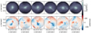 |
Fig. B.1. Six views of galaxy 377018 in snapshot 87 (from left to right). The top row shows the stellar mass per 0.25″ × 0.25″ in the field of view. The bottom row shows the mean line-of-sight velocity of the stellar particles. |
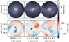 |
Fig. B.2. Same as Fig. B.1, three views of galaxy 377018 snapshot 87. The first three views in Fig. B.1 are chosen to be the most similar to the views in the x, y, z directions. |
Appendix C: SSP analysis with emission lines
We study the impact of excluding emission lines (ELs) when retrieving stellar population contributions in the spectra. In this test we run PYPIPE3D on a subsample of 100 simulated galaxies twice, first adding the EL spectra and then without them. The subsample is selected to have a representative distribution in the M* − Re plane of the MaNGA sample. The difference between the recovered ages and metallicities in each case is then used as an indicator of the bias introduced in SSP fits by the ELs. We calculate the EL contribution as in Ibarra-Medel et al. (2019) and downgrade its spectral resolution to MaNGA’s typical values before adding it to the stellar continuum spectra. While the resulting spectra look realistic, the EL spectra may not be reliably modelled, and therefore we do not pursue a further analysis of the ELs. An example of the spectra with the added contribution of the ELs is shown in Fig. C.1.
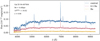 |
Fig. C.1. As in Fig. 5, but for the mock spectra with emission lines of a simulated galaxy at its centre, 0.5 Re, and 1 Re. |
Similar to the analysis in Sect. 4.2, we plot the difference between the mean ages and metallicities derived from the spectra within 1Re including ELs and those that do not include ELs for the same galaxies. As we are interested in the effect of ELs in the spectra and some of our 100 galaxies may have only weak ELs or no ELs, we identify the peak flux ratio between the spectra with and without the ELs within Re for each galaxy. While galaxies with weak ELs seem unaffected (scatter limited to ±0.5 dex), galaxies with strong ELs tend to lead to younger and more metal-poor estimations than when ELs are not included (Fig. C.2). While this effect is systematic in metallicity, the age estimations are more robust but with a larger scatter. The most extreme cases have a deviation of |Δlog(Age)| ∼ 0.4. At 2 Gyr; where the deviations are greater and more frequent, the ages can be estimated to be ∼1.2 Gyr younger. The correlation of this effect with age is evident since galaxies with young stellar populations will have young massive stars capable of ionizing the surrounding gas, thus producing emission lines. While this test shows how emission lines can impact in the SSP fitting, a more detailed study on the performance of PYPIPE3D is beyond the scope of this work.
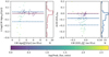 |
Fig. C.2. Difference retrieving ages and metallicities (left and right panels, respectively) with PYPIPE3D introduced by including emission lines in the spectra. The colour-coding is determined by the peak flux ratio between the spectra with and without the emission lines. The median of the differences is shown with a solid blue line, while the 20th and 80th percentiles are shown with dashed blue lines. |
Appendix D: Metallicity excess in stellar particles
The metallicities of the TNG50 stellar particles may have values above the upper limit of the MaStar_sLOG template. These values are not properly represented by the template, resulting in a underestimation of the average metallicity of the galaxy. We analyse how frequently the simulated galaxies have particles with metallicities above the threshold given by Zthres = max(ZSSP)+ΔZ, where max(ZSSP) = 0.4 is the maximum metallicity (Z) in the template and ΔZ = 0.05 is half the difference between the highest metallicity in the template and the one immediately before it. We consider that particles with metallicities above Zthres are underestimated when constructing the mock datacube.
Figure D.1 shows the fraction of stellar particles per galaxy in the MaNGIA sample where the metallicity exceeds Zthres and its dependence with stellar mass. For each galaxy, we considered all the particles identified with the subfind algorithm, which may not coincide with those in the field of view of the mock datacube. There is a clear dependence between stellar mass and high metallicity.
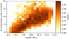 |
Fig. D.1. Fraction of stellar particles per galaxy in the MaNGIA sample where the metallicity exceeds Zthres (see text) and its dependence on stellar mass. N is the number density of galaxies per bin. |
All Tables
All Figures
|
Fig. 1. Distances in the mass-radius plane between MaNGA galaxies and their assigned TNG galaxy pair. From left to right: cumulative percentage of galaxies at a distance given by Eq. (1). Histogram of distances with galaxies paired with three repetitions. Histograms of the differences in the mass and radius components in d. The majority of MaNGA galaxies are allocated a TNG pair that is within a relative difference of 25% in the mass-radius plane. |
| In the text | |
|
Fig. 2. Matched properties of the MaNGIA sample. Left panel: Distribution of mass and effective radius (M* − Re plane) of the TNG galaxies in the matched sample, colour-coded by redshift. The black contours indicate the density of galaxies in the MaNGA M* − Re plane. Right panel: Mass vs. redshift of the TNG galaxies in the matched sample. The colour-coding indicates the MaNGA subsamples: galaxies in the Primary sample in red, Secondary sample in blue, and Color-Enhanced sample in yellow. The contours show the distribution of the MaNGA galaxies in the plane. |
| In the text | |
|
Fig. 3. Scheme followed to build a MaNGA-like datacube from a TNG50 simulated galaxy. Each step is described in Sect. 3 |
| In the text | |
|
Fig. 4. Fiber arrays used by MaNGA. Outer fibres of each MaNGA IFU bundle are shown in a different colour and a thick line, while circles with a thinner line width show the other two dithers for the same IFU. Large bundles have the same fibre array than smaller bundles, with additional rings of fibres in the outer parts. The inner-most fibres (IFU-19, light green) are shared by all the bundle sizes. |
| In the text | |
|
Fig. 5. Three simulated galaxies with stellar masses 109 M⊙, 1010 M⊙, and 1011 M⊙ show the mocking process. Panels on the left-hand side show the stellar mass density of the galaxies, while the central panels show their spectra at different radii (centre in blue, 0.5Re in red, and 1Re in yellow). Squared panels on the right-hand side show the stellar properties derived directly from the particles (top row for each galaxy) and recovered from the spectral cubes with PYPIPE3D (bottom row for each galaxy). From left to right, these panels show the V-band reconstructed image (mass density for the particle maps), luminosity-weighted age, luminosity-weighted metallicity, LsOS velocity, and velocity dispersion. As galaxy mass increases, the spectra are redder. Stellar maps are, in general, properly recovered. |
| In the text | |
|
Fig. 6. Difference between the intrinsic and assigned mean LW-age and metallicity (top and bottom, respectively, both in log-scale) within 1Re per galaxy (dots), calculated from the respective 2D maps. The yellow solid and dashed lines indicate mean and standard deviation of the differences of the complete set of galaxies. While ages are slightly younger after being assigned, metallicities show a greater negative deviation from the intrinsic values. |
| In the text | |
|
Fig. 7. Differences in age, metallicity, and extinction recovered by PYPIPE3D. The difference Δ is calculated as recovered-assigned for age and metallicity [dex] and as recovered-intrinsic for Av. The panels show the number density of galaxies of the differences across each parameter. The solid and dashed cyan lines show the mean and standard deviation of the differences, respectively, while the dashed magenta lines show 2σ deviations from the mean. An age-metallicity degeneracy is seen as PYPIPE3D tends to recover systematically younger ages and higher metallicities than expected. However, the recovered values are within the expected errors of 0.1 dex. As expected, extinction is increasingly underestimated as its value grows. |
| In the text | |
|
Fig. 8. Left panel: differences between intrinsic and recovered velocity dispersions as Fig. 7. Right hand-side panel: differences in extinction as a function of redshift. |
| In the text | |
|
Fig. 9. Simulated and observed recovered maps. The left panels show ten TNG50 recovered stellar population and kinematic maps. From top to bottom in each subpanel: the V-band reconstructed image, LW-age, LW-metallicity, LOS velocity, and velocity dispersion maps. The right panels show the MaNGA counterparts of each of the galaxies in the left panels. These examples were chosen to represent ten regions of the M* − Re: five mass bins (delimited by 109.25, 109.75, 1010.25, and 1010.75 M⊙), which correspond to the columns, with increasing mass from left to right, and two Re[kpc] regions per mass bin (rows, increasing size from bottom to top). |
| In the text | |
|
Fig. 10. TNG50 galaxies in the M* − Re plane (top) and their MaNGA counterparts (bottom). The galaxies are colour-coded from left to right by their mean LW-age, LW-metallicity, LOS maximum velocity, dispersion, and projected V/σ calculated within 1 Re from the recovered maps. The trends seen in the observed sample are replicated in the simulated sample with a greater dependence with galaxy size rather than mass. Although there is a discrepancy between the maximum values in dispersion and minimum values in age, the galaxies with these values lie in analogous regions of the plane. |
| In the text | |
|
Fig. 11. Median luminosity-weighted age (top panels) and metallicity (bottom panels) per mass bin at increasing radii for MaNGA galaxies (green) and TNG50 fully mocked with PYPIPE3D (solid magenta line). The median values for the TNG50 intrinsic and assigned maps are shown with dashed and dot-dashed lines to compare the median shift produced by the mocking process. The shaded areas span from the 20th to the 80th percentile. |
| In the text | |
|
Fig. 12. As in Fig. 11, but taking the mean age and metallicity per galaxy up to 1Re. The solid and dashed lines represent the median age (top panel) and metallicity (bottom panel) per stellar mass bin of the central and satellite galaxies, respectively. TNG50 galaxies are plotted in magenta, while MaNGA galaxies are plotted in green. |
| In the text | |
|
Fig. 13. Difference in the LW-age (top) and metallicity (bottom) obtained with MaStar_MA19 and MaStar_sLOG templates. The properties were calculated as the mean values within 1 Re from the assigned maps. While the metallicities are comparable, the assigned ages tend to be older when using the MaStar_MA19 template. |
| In the text | |
|
Fig. B.1. Six views of galaxy 377018 in snapshot 87 (from left to right). The top row shows the stellar mass per 0.25″ × 0.25″ in the field of view. The bottom row shows the mean line-of-sight velocity of the stellar particles. |
| In the text | |
|
Fig. B.2. Same as Fig. B.1, three views of galaxy 377018 snapshot 87. The first three views in Fig. B.1 are chosen to be the most similar to the views in the x, y, z directions. |
| In the text | |
|
Fig. C.1. As in Fig. 5, but for the mock spectra with emission lines of a simulated galaxy at its centre, 0.5 Re, and 1 Re. |
| In the text | |
|
Fig. C.2. Difference retrieving ages and metallicities (left and right panels, respectively) with PYPIPE3D introduced by including emission lines in the spectra. The colour-coding is determined by the peak flux ratio between the spectra with and without the emission lines. The median of the differences is shown with a solid blue line, while the 20th and 80th percentiles are shown with dashed blue lines. |
| In the text | |
|
Fig. D.1. Fraction of stellar particles per galaxy in the MaNGIA sample where the metallicity exceeds Zthres (see text) and its dependence on stellar mass. N is the number density of galaxies per bin. |
| In the text | |
Current usage metrics show cumulative count of Article Views (full-text article views including HTML views, PDF and ePub downloads, according to the available data) and Abstracts Views on Vision4Press platform.
Data correspond to usage on the plateform after 2015. The current usage metrics is available 48-96 hours after online publication and is updated daily on week days.
Initial download of the metrics may take a while.