| Issue |
A&A
Volume 671, March 2023
|
|
|---|---|---|
| Article Number | A156 | |
| Number of page(s) | 13 | |
| Section | Interstellar and circumstellar matter | |
| DOI | https://doi.org/10.1051/0004-6361/202245383 | |
| Published online | 21 March 2023 | |
Cosmic-ray sputtering of interstellar ices in the electronic regime
A compendium of selected literature yields
1
Institut des Sciences Moléculaires d’Orsay (ISMO), UMR8214, CNRS, Université Paris-Saclay,
Bât 520, Rue André Rivière,
91405
Orsay, France
e-mail: emmanuel.dartois@u-psud.fr
2
Laboratoire de physique des deux infinis Irène Joliot-Curie,CNRS-IN2P3, Université Paris-Saclay,
91405
Orsay, France
3
Centre de Recherche sur les Ions, les Matériaux et la Photonique, CIMAP-CIRIL-GANIL, Normandie Université, ENSICAEN, UNICAEN, CEA, CNRS,
14000
Caen, France
4
Institut de Minéralogie, de Physique des Matériaux et de Cosmochimie, CNRS, MNHN, Sorbonne Univ.,
75005
Paris, France
5
Université Grenoble Alpes, IPAG,
38000,
Grenoble, France ;
CNRS, IPAG,
38000
Grenoble, France
Received:
5
November
2022
Accepted:
20
January
2023
Aims. With this article, we aim to provide the sputtering yields for molecular species of potential astrophysical interest and in the electronic regime of interaction characteristic of cosmic rays. We specifically target molecules that are constitutive of interstellar ice mantles.
Methods. We used a compendium of existing data on electronic sputtering to calculate the prefactors leading to the generalisation of the stopping-power-dependent sputtering yield for many species condensing at low temperature. In addition, we present new experimental results to constrain the yield for solid CH4, C6, and CH3CN.
Results. Electronic sputtering is constrained using literature data for H2, HD, D2, Ne, N2, CO, Ar, O2, Kr, Xe, CO2, SO2, NH3, S, H2O, D2O, CH3OH, Leucine, C20H12, C24H12, and C60. A first-order relation with the sublimation enthalpy is derived, which allows us to predict the sputtering yield within an order of magnitude for most species. The fluctuations around the mean are partly assignable to the differences in resilience towards radiolysis for individual species, and partly to the micro-physics details of the energy transfer to the lattice.
Key words: astrochemistry / cosmic rays / ISM: lines and bands / molecular processes / solid state: volatile
© The Authors 2023
 Open Access article, published by EDP Sciences, under the terms of the Creative Commons Attribution License (https://creativecommons.org/licenses/by/4.0), which permits unrestricted use, distribution, and reproduction in any medium, provided the original work is properly cited.
This article is published in open access under the Subscribe to Open model. Subscribe to A&A to support open access publication.
1 Introduction
In dense phase regions, where the solid phase is of increasing importance in the chemical evolution of the medium, observations show that efficient mechanisms are at work to replenish the gas phase with species otherwise condensed on more refractory dust particles. The presence of high-energy radiation fields (e.g. UV, X) and cosmic-ray particles interacting with the gas and dust particles influences their physical and chemical evolution. The desorption of many observed species from the solid phase, which is induced by photons and/or high-energy particles, needs to be quantified in order to account for their contribution to the enrichment of the gas phase. The interaction of high-energy particles with solids in the electronic regime of interaction leads to sputtering, both because of the resulting heating of the entire grain (e.g. Leger et al. 1985) over long timescales after deposited energy is relaxed for small grains, and because of more local heating at early times in the energy cascade of the solid lattice. This latter induces a so-called thermal spike effect (e.g. Dufour & Toulemonde 2016; Johnson et al. 2013; Sigmund 1987, and references therein), in which a temperature rise occurs typically within less than 100 ps in the bulk close to the ion trajectory. The goal of the present article is to provide the sputtering yields in the electronic regime of the interaction of ions with solids, which is the regime adapted to describing Galactic cosmic rays (GCR) and is therefore of potential astro-physical interest. We used a compendium of existing data on electronic sputtering to calculate the prefactors leading to the generalisation of the stopping-power-dependent sputtering yield for many species condensing at low temperature. In addition, we present new experiments to constrain the yields of CH4, C6H6, and CH3CN. A first-order relation relating the sputtering rates with the sublimation enthalpy of the condensed species is shown, with variations partly assignable to the differences in resilience towards radiolysis for individual species.
2 Sputtering law
At low temperature and normal incidence, a functional (empirical law) describing the sputtering yield for a majority of molecular solids normal to the surface can be approximated to first order by the simple equation
 (1)
(1)
where Ytot is the total number of molecules (or rare gas atoms) ejected per incident ion, and Sn and Se are the ion stopping power in the so-called nuclear and electronic regimes. We make use of the stopping power expressed in this article in units of eV/(1015 molecules cm−2) for molecular solids and of eV/(1015 atoms cm−2) for rare gases and atomic solids, as widely used in the literature (e.g. Dartois et al. 2015; Raut & Baragiola 2013; Johnson et al. 2013; Schou & Pedrys 2001; Brown et al. 1984, and references in the abundant literature in the following). This stopping power unit allows us to compare the results on a scale that becomes independent of the target density. It also provides a yield per entity considered (i.e. molecule, or atoms for rare gases), which simplifies the interpretation.  and
and  are the nuclear and electronic sputtering prefactor, respectively. A more general empirical fit for water ice is given in Johnson et al. (2013), including angular dependence and thermal activation at high temperatures1. Here, we only use data where Se/Sn > 10 (with the corollary that
  ), and so Eq. (1) can be simplified as
 (2)
(2)
and is therefore clearly dominated by the electronic stopping power of ion particles.
 |
Fig. 1 Influences of the different elements in processes associated with cosmic rays represented as fractional proportions on a log scale. Left: Galactic cosmic-ray abundance. Middle: relevance of the cosmic-ray elements in processes proportional to Z2, i.e. typically the radiolytic destruction of ices constituents. Right: relevance of the cosmic-ray elements in processes proportional to Z4, i.e. typically associated with the electronic sputtering mechanisms discussed in this article. |
3 Relative importance of cosmic-ray elements
The sputtering yields, once determined as a function of the stopping power, can be used in models to simulate the sputtering process in interstellar space, taking into account the composition and flux of cosmic rays. The Galactic cosmic-ray abundances of elements from hydrogen to nickel are represented as fractional proportions on a log scale in the left panel of Fig. 1. Adopted Galactic cosmic-ray abundances of H and He are from Wang et al. (2002), those of Li and Be are from de Nolfo et al. (2006), and those above Be are from George et al. (2009). Hydrogen and helium abundances dominate in cosmic rays. The electronic stopping power, that is, the energy deposition, of a projectile in a given material scales with the projectile atomic number (Z) to the power of two (e.g. Chabot 2016; Ziegler et al. 2010; Bringa & Johnson 2003; Sigmund 1995). For astrophysical processes with ices involving an energy dependence proportional to Se (or close to that), such as radiolysis processes, heavier elements such as C, O, Ne, Mg, Si, and Fe play a significant role despite their lower abundance. This is what is shown in the middle panel of Fig. 1. In the case of the ice sputtering explored here, the relative contributions of the various cosmic-ray species evolve as the square of Se, therefore the dependency is in Z4. The heavier elements are then dominant in the effectiveness of the sputtering process, and iron becomes the most important cosmic-ray element, as shown in the right panel of Fig. 1. This is why it is important to perform measurements experimentally over a broad range of stopping powers, and to model the effect of the complete cosmic-ray distribution of elements, and not only H and He, in the case of sputtering.
4 Literature data and experiments
Literature data were explored for all the species presented in this article, and are scaled to a common electronic stopping power unit for comparison (eV/(1015 molecules cm−2)). If not provided in the original articles, we recalculate the stopping power in the electronic regime (as well as the nuclear stopping power in order to ensure we only consider experiments where the electronic stopping power dominates) using the SRIM (Ziegler et al. 2010) package.
The ice sputtering yields that we selected in this article were measured in the semi-infinite limit, i.e. with thick ice targets with respect to the number of sputtered molecules, unless stated otherwise. The origins of the sets of data that we use are explained in the following subsections. Many more irradiation experiments exist in the literature. However, the ones presented are selected because they provide absolute sputtering yield values.
H2, HD, D2
Sputtering of solid hydrogen molecules and iso-topologues (H2, HD, D2) irradiated by keV H+ were reported by Schou et al. (2002). D2 sputtering was explored with H+ in the keV range by Stenum et al. (1991a) and with 2 keV electrons by Børgesen & Sørensen (1982).
N2
Published yields for molecular nitrogen show marked variations. Its electronic sputtering yield has been found to be much less than that of dioxygen in measurements by Johnson et al. (1991) and Gibbs et al. (1988). The magnitude of the sputtering yield measured by other authors (Pirronello et al. 1981; Stenum et al. 1991b) is higher than expected when compared to the extrapolation of the other set of data and using a quadratic behaviour for the sputtering yield; these data sets seem not to reconcile with each other. In May 2019, 15N2 was available on an injection line to be used for an upcoming experiment on the simulation of isotopic anomalies in extraterrestrial organic matter produced by cosmic-ray irradiation of Solar System ices. In order to provide additional constraints on previous data sets, we measured the solid 15N2 sputtering yield at higher stopping power in order to add an additional point in the sputtering yield dependence on this latter parameter. The details of this yield determination are given in Dartois et al. (2020). When reported as a function of the electronic stopping power, this sputtering yield is in better agreement with the quadratic behaviour extrapolation from the data of Pirronello et al. (1981) and Stenum et al. (1991b) than with the Johnson et al. (1991) data alone.
CO
Carbon monoxide has been studied in many experiments. The data used in the compendium presented here were retrieved from reviews of CO data, such as in Brown et al. (1984), Johnson et al. (2013), and references therein. Data from Schou & Pedrys (2001) with 6–9 keV H+,  , and
, and  projectiles were added. Additional high-energy measurements with 50 MeV and 537 MeV Ni ions (Seperuelo Duarte et al. 2010) as well as 38 MeV Ca and 33 MeV Ni (Dartois et al. 2021) complete the already large data set. The data therefore span three orders of magnitude in stopping power. This is one of the best constrained quadratic dependencies on stopping power for electronic sputtering.
CH4
The CH4 ice sputtering yield was measured at the heavy-ion accelerator Grand Accélérateur National d’Ions Lourds (GANIL) during a swift ion irradiation experimental campaign with 56Fe10+ projectiles in June 2022. Details on the yield determination are given in Appendix A.
O2
MeV proton and helium ions were used to monitor the electronic sputtering of dioxygen by Johnson et al. (1991) and Gibbs et al. (1988). The proton experiments with the lowest stopping power show a linear dependency, whereas the nuclear stopping power does not contribute significantly to the total stopping power. This behaviour is attributed by Famá et al. (2007) to repulsion of ions in the ionisation track of the projectile, which, at low velocities, is augmented near the surface due to the additional ionisation resulting from electron captures. Other yield measurements performed earlier by Famá et al. (2002) with 100 keV protons using a quartz cell and mass spectrometer (that we corrected by the cosine of the 45° irradiation angle) show a higher sputtering efficiency than for the Johnson et al. (1991) and Gibbs et al. (1988) previous H+ measurements, with stopping power in the same range. These add to the dispersion in the evaluation of the prefactor for oxygen. Ellegaard et al. (1986a) showed that for O2, the keV electron sputtering yield is more linear than proportional to the square of the stopping power, and we do not include these measurements. In the electron irradiation case, these latter authors favour a sputtering yield driven by low-energy collision cascades initiated by dissociative recombination.
Ne, Ar, Kr, Xe
Yields for neon electronic sputtering by keV protons were extracted from measurements presented by Schou (1988) and Ellegaard et al. (1986b). Argon sputtering measurements were retrieved from MeV proton, di and trihydro-gen cation, and helium ion experiments (Besenbacher et al. 1981; Reimann et al. 1984b; Schou 1987; O’Shaughnessy et al. 1986). Krypton sputtering measurements were retrieved from several keV di and trihydrogen cations, and 30 keV helium ion experiments (Schou 1987; O’Shaughnessy et al. 1986). Xenon yields are obtained from MeV ion experiments (Bøttiger et al. 1980; Schou 1987) and 30keV helium ions (O’Shaughnessy et al. 1986).
As seen in Fig. 2, rare gases seem to display a particular behaviour, which is closer to a linear dependency of the yield on the stopping power, even for measurements where the electronic stopping power clearly dominates. Only Xe seems to show apseudo quadratic behaviour. This should be furtherinvestigated with additional measurements.
CO2
Carbon dioxide sputtering yield measurements were taken from Raut & Baragiola (2013), who used 100 keV protons irradiations, and Brown et al. (1982), who used H+, He, C+, and O+ ions, the results of which are also discussed in Brown et al. (1984). Recent sputtering yields with heavy ions in the MeV/u range were also added (Ni, Xe, Ti; Seperuelo Duarte et al. 2009; Mejía et al. 2015; Rothard et al. 2017; Dartois et al. 2021); these give rise to the points at high stopping power.
S, SO2
Elemental sulfur (S8) sputtering yields using several keV ion irradiations were measured by Chrisey et al. (1987). We selected the proton and helium ions, which are the only ones for which the electronic energy stopping power dominates in these experiments. MeV helium ion experiments by Torrisi et al. (1986) were also retrieved. Sulfur dioxide irradiations were conducted using 1.5 MeV He to 25 MeV F ions by Melcher et al. (1982) and Lepoire et al. (1983), and with 50 and 750 keV hydrogen ions, and 1.5 MeV hydrogen molecules, helium, oxygen, and argon ions by Lanzerotti et al. (1982).
NH3
The absolute sputtering yield for ammonia ice was measured with 1.5 MeV proton and neon ions by Lanzerotti et al. (1984). The error bars for this species appear moderate simply because of the lack of additional measurements, which would probably provide a larger scatter.
CH3OH
The sputtering yield for methanol was measured using 95 MeV swift xenon ion projectiles (Dartois et al. 2019). Additional measurements are required to better constrain the prefactor.
CH3CN
The sputtering yield for acetonitrile was measured experimentally using 33 MeV swift 56Fe10+ ion projectiles at GANIL in June 2022. The details of the determination of the CH3CN sputtering yield are given in Appendix C.
H2O, D2O
Water ice sputtering has been the subject of numerous investigations, as it represents a major ice matrix for most cold astrophysical objects from natural satellites and comets to interstellar dust grains in dense cloud regions. Many articles have been dedicated to the nuclear stopping power in view of its importance for planetary cold satellite surfaces. In the following, we refer to specific experiments when the electronic sputtering largely dominates the energy deposition and, when the information is available, the ice thickness is sufficient to have reached a plateau (i.e. the semi-infinite sputtering yield). Irradiations of water ice were performed using, as projectiles, 1 MeV helium and nitrogen ions by Bøttiger et al. (1980); 1.6–25 MeV fluor ions (Seiberling et al. 1982; Cooper & Tombrello 1984); keV to MeV protons, helium, carbon, and oxygen ions (Brown et al. 1980, 1982, 1984); 15–50 keV proton,  , and
, and  (Rocard et al. 1986); 15–50 keV helium and hydrogen (Bénit et al. 1987); 10–90 keV proton, deuteron, and helium ions (Shi et al. 1995); 1 MeV helium and 1.6–25 MeV fluor ions (Cooper & Tombrello 1984); 5–90 keVu−1 protons and helium ions (Baragiola et al. 2003); 46 MeV nickel, 81 MeV tantalum (Dartois et al. 2015), and 95.2MeV xenon (Dartois et al. 2018). The scatter in the results is higher than for example CO, leading to a higher uncertainty in the sputtering prefactor calculation. The heavy water sputtering yield was also measured with 30 and 50keV helium by Chrisey et al. (1986), as well as 1.5 MeV helium and neon ions by Reimann et al. (1984a).
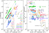 |
Fig. 2 Left: compendium of the sputtering yields Y obtained from the literature as a function of the electronic stopping power Se, to which are added our recent N2 measurement. The upper left dashed and dotted lines show the expected behaviour if the sputtering evolves linearly or quadratically, respectively, with the stopping power. The quadratic fit to each set of data for molecular systems and rare gases is over-plotted with dotted lines for comparison. Right: same data, assuming a quadratic dependency of the electronic sputtering yield on the stopping power, i.e. dividing the yield by Se2. Under this representation, a quadratic behaviour appears as a flat line, represented with dotted lines, and allows us to derive the sputtering yield prefactor |

Leucine
The sputtering of large molecules of biological interest has been thoroughly explored experimentally, mainly as a way to put such molecules in the gas phase for analytical purposes. If many experiments with swift ions do exist, only a handful of them have been sufficiently quantitative to allow an estimate of the absolute sputtering efficiency yield. Håkansson et al. (1988) used 78.2 MeV iodine, 48.7 MeV brome, 35.7 MeV nickel, and 19.7 MeV sulfur ions to irradiate leucine (C6H13NO2) and measured the absolute sputtering yield using a collector method. By comparing the measured absolute values to positive ions, these authors also confirm that the neutral sputtering yields are many orders of magnitude higher than those of secondary ions.
C6H6
The sputtering yield for benzene was measured experimentally using 33 MeV swift 56Fe10+ ion projectiles at GANIL in June 2022. Details of the determination of C6H6 sputtering yield are given in Appendix B.
C20H12 and C24H12
The sputtering yield for pery-lene and coronene was measured experimentally by Dartois et al. (2019).
C60
One experiment reports the electronic sputtering yields of the buckminsterfullerene C60 for 130 MeV Ag and 80–200 MeV Au projectiles (Ghosh et al. 2004). A yield of 500±75 C60/ion is given for the 200 MeV Au experiment, and we extract yields from published 130MeV Ag and 80MeV Au experiments by Ghosh et al. (2003). These experiments would require additional constraints, as it is assumed that most of the ejected systems remain intact. The absolute values are difficult to measure, but experiments on polyaromatic-molecule systems for swift heavy ions seem to show that even if fragmentation occurs, a large fraction of the molecules ejected are intact and they also confirm that the sputtering yields of neutral species are many orders of magnitude higher than for ion species (Breuer et al. 2016).
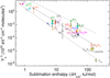 |
Fig. 3 Sputtering prefactor from Eq. (1) obtained from the fitting to the data presented in Fig. 2, reported as a function of the sublimation enthalpy of the considered species. A sputtering yield evolving quadratically with the stopping power has been adopted. There is a first-order correlation of |

5 Results
5.1 Compendium
The compendium of stopping-power-dependent yields for rare gases and molecular solids at low temperature is shown in Fig. 2 (left panel). The expected slopes representing a linear (Y ∝ Se) or quadratic ( ) behaviour on stopping power are plotted with dashed lines in the upper left for comparison. One common stopping power Se unit as calculated using the SRIM code (Ziegler et al. 2010) is given per atom in the target (10−15 eV cm2 atom−1) as to first order the stopping power scales with the atomic density for equivalent atoms. We decided to represent yields in terms of stopping power unit per molecule or species for evident consideration of the molecular solid entities in astrophysics. Following Eq. (2), the data are divided by
  and fitted to provide prefactors
  and show their dispersion with respect to the quadratic dependency on stopping power when large sets of data are available (Fig. 2, right panel). The corresponding fits are also over-plotted with dashed lines to the data from the literature in the left panel. The constrained prefactors are summarised in Table 1. When the nuclear contribution to the sputtering yield remains important (i.e. if the crossing point between the nuclear and electronic range sputtering slopes is high because
  is high), or if the behaviour does not follow a quadratic power law within the existing measurement range, then the calculated
  constant will be overestimated by the fitting procedure, and we therefore give this value as an upper limit (e.g. for Ne). Sputtering data clearly showing a Y/Se behaviour include the neon case. In the absence of further constraints on their behaviour, we provide upper limits to
  for the rare gases.
5.2 Relation to the sublimation enthalpy
The electronic sputtering prefactor ( ) in Eq. (1) is reported as a function of the sublimation enthalpy of the molecular solids in Fig. 3. There is a first-order correlation of
  with a power law of ΔHsub, which is indicated by the dashed line and framed by the dotted lines. The fitting to the complete set of data allows us to define that
  , where n = −2.9 ± 0.8 at 3 σ. Excluding the four highest-molecular-weight species would provide a slope that is slightly less steep, with n = −2.2 ± 0.6.
This first-order correlation might reflect the fact that the highest criterion for the magnitude of the electronic sputtering for such solids is the sublimation energy that must be overcome after the energy is deposited over a short timescale in the molecular lattice within the so-called thermal spike effect (e.g. Dufour & Toulemonde 2016, and references therein), in which the temperature rise occurs typically within less than 100 ps in the bulk. We note that this is only a very first-order correlation, as relatively large variations are observed at a given ΔHsub because of the influence of many other parameters, among which the degree of electron phonon coupling and specific heat of the solid, which are taken into account in thermal spike models, and also the radiolysis efficiency for the considered species. If the radiolytic efficiency becomes too high, for larger species, the yield will decrease more rapidly than the correlation observed with the sublimation enthalpy, as suggested by the apparent change in the slope of the prefactor in Fig. 3 for the larger species, or mainly ejected fragments will be produced. The case of mixtures will also modify the yields and these will rely on the details of the energy transfer among species and newly opened radiolytical/chemical routes. In astrophysical media, if the species are embedded in a dominant matrix, the sputtering yield of the host is expected to be close to the pure species, but must be recorded to take into account the difference in stopping power and possible new routes for radiolytic processes occurring during the energy deposition (e.g. Dartois et al. 2020, 2019). When dealing with ice mixtures not dominated by one species, and especially if these species have very different enthalpies of sublimation, the sputtering yield evolution we deduce from pure species will serve as a guideline, but dedicated experiments must be conducted with the expected relative proportions in order to take into account both the lattice change and also possible new routes for radiolysis.
Sputtering yield prefactors and adopted low-temperature sublimation enthalpies for the considered species.
5.3 Comparison with photodesorption
In interstellar space, cosmic rays directly contribute to sputtering. They also participate in the generation of a secondary vacuum Ultraviolet (VUV) photon field by interaction with the gas, which leads to ionisation and recombination, mainly of hydrogen. These secondary VUV photons also induce a photodesorption process after absorption of these photons in the electronic states of the species constitutive of the molecular or atomic solid. The photodesorption yields can be measured experimentally (e.g. Dupuy et al. 2017a; Carrascosa et al. 2020; Martín-Doménech et al. 2018; Westley et al. 1995; DeSimone et al. 2013; Cruz-Diaz et al. 2018, 2016; Öberg et al. 2007, 2009; Arakawa et al. 2000; Fayolle et al. 2011, 2013; Bertin et al. 2012, 2016; Chen et al. 2014; Muñoz Caro et al. 2010; Dupuy et al. 2017b; Féraud et al. 2019; Zhen & Linnartz 2014; Bahr & Baragiola 2012; Yuan & Yates 2013; Martín-Doménech et al. 2015; Basalgète et al. 2021). A relation between the measured cosmic ray ionisation rate ζ and the generated secondary VUV photon flux was estimated by Prasad & Tarafdar (1983) of 1350 VUV photons cm−2 for an ionisation rate of 1.7 × 10⁻¹⁷ s−1, and about 3130 photons cm−2 for an ionisation rate of 3 × 10⁻¹⁷ s−1 by Shen et al. (2004). For comparison of the relative importance of photodesorption versus cosmic-ray-induced desorption, we summarise photodesorption rates retrieved from the literature in Table 2 and Fig. 4. As the VUV flux in the dense regions of the ISM is thus linked to the cosmic-ray-induced ionisation rate, we report in Fig. 4 the equivalent rate assuming a mean value of about 920 photons cm−2 for an ionisation rate of 10−17 s−1. Although neon is clearly above the other photodesorption rates, there is no longer any clear trend with the sublimation enthalpy. The nature of the photon interaction with the individual species is very different from the thermal spike model for cosmic-ray sputtering, and is very specific not only to the electronic structure of the solids but also to the possible energy transfer after absorption of the VUV photons. Large variations in the measured rates are observed. Part of the variations may still be due to the distribution of VUV photons used in the different experiments.
5.4 Astrophysical sputtering rate
Converting the derived prefactors into an effective sputtering rate for astrochemical networks requires that the sputtering rates be integrated over the cosmic-ray fluxes. The sputtering rate by cosmic rays can be calculated by:
 (3)
(3)
where RateGCR(cm−2 s−1) is the resulting sputtering rate, and  (E, Z)[particles cm−2 s−1 sr−1/(MeV/u)] is the differential flux of the cosmic-ray element of atomic number Z, with a cutoff in energy Emin set at 100 eV. Moving the cutoff from 10 eV to 1 keV does not change the results significantly. The differential flux for different Z follows the observed relative GCR abundances from Wang et al. (2002) (H, He), de Nolfo et al. (2006) (Li, Be), and George et al. (2009) (>Be), as explained in more detail in Dartois et al. (2013). The integration is performed up to Ζ = 28, corresponding to Ni, and a significant drop in the cosmic abundance and therefore contribution is observed above that. The sputtering rate YCR(E, Z) follows from Eq. (2) and the prefactor derived from the present literature analysis and the calculated electronic stopping power Se using the SRIM code (Ziegler et al. 2010) as a function of atomic number Ζ and specific energy E (in MeV per nucleon). For the differential Galactic cosmic-ray flux, we adopt the functional form given by Webber & Yushak (1983) for primary cosmic-ray spectra using the leaky box model, also described in Shen et al. (2004),
 (4)
(4)
where C is a normalisation constant (= 9.42 × 10⁴, Shen et al. 2004). Under such parametrisation, the high-energy differential flux dependence asymptotically approaches a slope of −2.7. Unless close to a strong emitting source (like a supernova), the propagation of cosmic rays in the diffuse ISM (GALPROP model, e.g. Jóhannesson et al. 2016), the local ISM (e.g. Cummings et al. 2016; Bisschoff & Potgieter 2016), and in dense molecular clouds (e.g. Chabot 2016) flattens the distribution in the low energy range. To first order, the E0 form parameter allows us to adjust with a simple parameter the less understood low-energy cosmic-ray contribution, and thus influences the resulting ionisation rate; but a full propagation model can also be used (e.g. Chabot 2016), providing a better approximation of the relative ratio of contributions to sputtering for heavier cosmic rays, particularly in very dense regions of the cloud. Typical adopted conservative values for E0 to explore different propagated distributions are taken between 200 and 600 MeV u−1 (e.g. Shen et al. 2004). The ionisation rate (ξ2) corresponding to the same distribution can also be calculated (Sect. 4.4.2 in Dartois et al. 2013), and gives an observable that can be compared with astro-physical observations obtained in various environments (e.g. McCall et al. 2003; Geballe & Oka 2010; Indriolo & McCall 2012; Neufeld & Wolfire 2017; Oka et al. 2019). The sputtering rates for the main interstellar ice constituents, namely H2O, CO2, and CO, has been evaluated in such models using the estimated prefactors, and the corresponding ionisation rates derived. The results are presented in Fig. 5. In this plot, we put a (loose) upper limit on the range of validity of these calculations. Indeed, interstellar ice mantles appear above a visual extinction threshold (dependent on the considered dense cloud), and this sets an upper limit to the maximum ionisation rate for dense cloud regions where they reside. The ionisation rate cannot be set arbitrarily high, even close to a strong source, because of the minimum propagation through a few AV of matter.
Photodesorption rates from the literature.
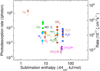 |
Fig. 4 Photodesorption rates from the literature reported as a function of enthalpy of sublimation. The variations in the absolute determination of the rate for various experiments are reported in Table 2. The right ordinate axis translates the rates into effective rates for a given ionisation rate ζ, assuming about 920 VUV photons cm−2 s−1 for an ionisation rate of ζ = 10−17 s−1. See text for details. |
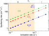 |
Fig. 5 Sputtering rate as a function of ionisation rate for H2O (blue), CO2 (red), and CO (green). The upper abscissa axis represents the approximate relation established between observed ionisation rate and the inverse of the visual extinction (e.g. Neufeld & Wolfire 2017). The arrow is shown to stress the fact that ices only appear above a visual extinction threshold (dependent on the particular dense cloud). This sets an upper limit to the maximum ionisation rate for dense cloud regions where they reside. The ionisation rate cannot be set arbitrarily high, even close to a strong source, as the cosmic rays spectrum is propagated (and therefore low energies attenuated) at least within a column density of matter corresponding to this minimum threshold AV. |
5.5 Cosmic-ray versus secondary VUV photon rates
The ratio of cosmic rays to photodesorption rates calculated for a cosmic ray distribution leading to an ionisation rate of 3 × 10⁻¹⁷ s−1 is presented in Fig. 6, corresponding to about 2760 cosmic-ray-induced secondary VUV photons s−1 cm−2 (see above); that is, the visual extinction is high, the external VUV field is attenuated by dust grains, ice mantles are developed, and the VUV photons to cosmic rays ratio is almost constant. As can be seen in Fig. 6, there is sometimes a large dispersion in the reported photodesorption yield. It is clear from this plot that for small species, cosmic rays and secondary VUV photons show comparable rates, but that cosmic rays dominate when species are bigger.
6 Conclusions
We report a compendium of absolute sputtering yield values derived by fitting data retrieved from the literature resulting from experiments involving the interaction of high-energy ions representative of the energy deposition in the electronic regime, such as is the case for cosmic rays. We focus on molecular solids of potential astrophysical interest, some constitutive of interstellar ice mantles. In addition, we add new experimental data to constrain the yield for solid CH4, CH3CN, C6H6 at high energy.
We fitted a quadratic model, allowing us to extract the sputtering yield prefactors for a simple description of the energy-dependent sputtering yield for 24 solids, with only upper limits for 4 of them.
Our most remarkable finding is that we show a tendency of the sputtering prefactor to correlate, to first order, with the enthalpy of sublimation of the considered solids. This can be used to predict the range in which the sputtering yield of other species should lie. This relation with the sublimation enthalpy supports the fact that the thermal spike model is a good description of the process, in which the energy is rapidly transferred to the lattice prior to sublimation of essentially neutral species. The fluctuations around the trend found may be imputable to many other competitive mechanisms at work, such as the radiolysis efficiency and details in the energy transfer to the lattice, which is strongly species dependent. The sputtering-yield pref-actors for the species considered can be used in astrochemical models. The trend with the sublimation enthalpy can be used to derive yields for new species, providing first-order sputtering rates that can be implemented in models in the absence of dedicated experimental results. These will also help in predictions of experimental parameters that can be used to better constrain yields using designed astrophysics experiments in the laboratory.
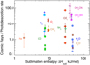 |
Fig. 6 Ratio of cosmic rays to photodesorption rates calculated for a cosmic ray distribution leading to an ionisation rate of 3 × 10⁻¹⁷ s−1, and corresponding to about 2760 UV photons s−1 cm−2. See text for details. |
Acknowledgements
This work was supported by the Programme National ‘Physique et Chimie du Milieu Interstellaire’ (PCMI) of CNRS/INSU with INC/INP co-funded by CEA and CNES. Experiments on CH4, C6H6, CH3CN were performed at GANIL. We thank T. Madi, J.-M. Ramillon, F. Ropars, A Sineau, F. Dardy, and P. Voivenel for their invaluable technical assistance. CAFDC acknowledges a RIN post-doc grant from Normandy Region.
Appendix A CH4 sputtering yield determination
The CH4 ice sputtering yield was measured at the heavy-ion accelerator Grand Accélérateur National d’Ions Lourds (GANIL) during the June 2022 swift ion irradiation experimental campaign. 56Fe10+ projectiles were accelerated at 39.25 MeV on the IRRSUD beam line. This beam was coupled to an ultrahigh vacuum chamber, the IGLIAS (Irradiation de GLaces d’Intérêt AStrophysique) setup, operating in the 10−9 mbar range for the considered experiment, holding an infrared transmitting ZnSe substrate window cryocooled at 10 K, on top of which the ice films are condensed (for details, see Augé et al. 2018). The ice films are produced by placing the cold window substrate in front of a deposition line where gas mixtures are injected. The targeted film thickness is in the micron range. At such thicknesses, the ion beam passes through the film with an almost constant energy deposition. At the considered ion energy, the stopping power is dominated by the electronic regime and amounts to Se = 1791 × 10−15eV cm2/CH4 molecule. In the following, we refer to ‘electronic stopping power’ for brevity. A Bruker Vertex 70v FTIR spectrometer with a spectral resolution of 1 cm−1 was used. The evolution of the infrared spectra was recorded at several fluences; the infrared transmittance spectra are recorded at 12° of incidence (a correction factor of 0.978 is therefore applied to determine the normal column densities).
As discussed in previous articles on the modelling of the evolution of ice mantles (Dartois et al. 2021, 2020, 2015), the column density of the ice films can be described —when exposed to ion irradiation— as a function of ion fluence (F) by a differential equation:
 (A.1)
(A.1)
where N is the CH4 column density, σdes is the ice effective radiolysis destruction cross-section (cm2), and  is the semi-infinite (thick film) sputtering contribution in the electronic regime to the evolution of the ice column density. This is multiplied, to first order, by the relative fraction (f) of the considered species (here named x) with respect to the total number of molecules and radicals in the ice film, which are estimated from their measured column densities, as follows
 (A.2)
(A.2)
The first term −σdesN in the right hand side of the equation is a bulk process affecting all depths in the film, whereas the second term  affects the surface up to a depth corresponding to a column density of ≈ Nd. When the ice film is thin (column density N ≲ Nd; Nd being the semi-infinite ‘sputtering depth’), the removal of molecules by sputtering follows a direct impact model, that is, all the molecules within the sputtering area defined by a sputtering ‘effective’ cylinder are removed from the surface. The apparent sputtering yield, as a function of thickness, is modelled to first order to estimate the corresponding sputtering depth by an exponential decay, leading to the 1 – e(−N/Nd) correcting factor applied to
  . A schematic view of such a simplified cylinder approximation is shown in Fig.1 of Dartois et al. (2018). The sputtering cylinder is defined by a radius rs (defining an effective sputtering cross section σs) and a height d (related to the measured sputtering depth). These parameters are calculated from the measurement of Nd and
  . The column densities of the molecules are followed experimentally in the infrared via the integral of the optical depth (τv̄) of a vibrational mode, taken over the band frequency range. The band strength value (A, in cm/molecule) for a vibrational mode has to be considered. The evolution of the methane column density is followed using the v4 band around 1300 cm−1 integrated band strength of A ≈ 8 × 10⁻¹⁸cm/CH4 (Bouilloud et al. 2015). This band is more suitable here than the 3000 cm−1 ν4 band because of the absence of strong overlap with the contribution from the radiolysis products of the irradiation. The results are anchored to the adopted A values and should be modified if another reference value is favoured.
The evolution of the infrared spectra upon ion irradiation shows three stages that are much better understood when the data are plotted showing dN/dF as a function of column density, rather than column density as a function of fluence, evolving over several decades. We clearly see in Fig. A.2 that the evolution of dN/dF departs from the ideal model of Equation A.1, in particular at low fluence. At the beginning of irradiation, the ice film evolves towards the compact amorphous structure with the first ions impinging the freshly deposited ice film. Therefore, the molecular environment and phase is modified and/or compacted. The oscillator strength of the measured transitions in the infrared and/or the refractive index of the ice are slightly changing. As a consequence, the apparent dN/dF evolution is rapid. At the considered stopping powers for the ions, this is stabilised after a fluence of a few 1011 ions/cm2, and the observed behaviour of dN/dF better follows the expectation of the model. This early phase of the irradiation cannot be safely used to monitor the column-density variations as both the molecule column density and the infrared band strength vary, leading to unpredictable changes, and they are discarded from the fits used to extract the model parameters (in the figures they are represented by light colours in the dN/dF plots). Including these points in the fit leads to misestimation of the radiolysis destruction cross-section. In the second evolution stage, the film can be considered semi-infinite with respect to the sputtering and dN/dF evolves as a slope combining the radiolysis of the bulk and semi-infinite sputtering. In the later phase, the film becomes thin with respect to the semi-infinite sputtering depth (Nd) of individual ions. dN/dF decreases accordingly with a linear and exponentially convolved behaviour.
Fits of Equation A.1 are shown in the middle panels of Fig. A.2. Best parameters were retrieved with an amoeba method minimisation to find the minimum chi-square estimate on the model function. The fitted output parameters, namely σdes,  , and Nd, are 7.0 ± 0.8 × 10⁻¹⁴ cm2, 1.2 ± 0.08 × 10⁵ CH4/ion, 2.0 ± 0.2 × 1017 cm−2, respectively, with the uncertainties being estimated at two times the reduced chi-square value obtained in the minimisation.
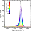 |
Fig. A.1 Infrared spectra of the v4 vibrational mode for the CH4 ice experiment with 39.25 MeV 56Fe10+ ions. The inserted colour code gives the corresponding irradiation fluence. |
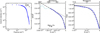 |
Fig. A.2 CH4 sputtering yield determination. Left panel: CH4 column-density evolution measured with the v4 mode spectra as a function of 56Fe10+ ion fluence for a CH4 ice film deposited and measured at 10 K. Middle panel: Experimentally measured differential evolution of -dN/dF as a function of column density, to be compared to equation A.1. A fit of the equation to the data is shown as a black long-dashed line, and a fit not taking into account the finite depth of sputtering is shown with a short-dashed line. Right panel: Sputtering yield evolution as a function of column density; over-plotted are the infinite thickness yield (dashed lines) and adjusted exponential decay (long-dashed lines). See text for details. |
Appendix B C6H6 sputtering yield determination
The application of the column density of the ice films described by Equation A.1 recorded directly by infrared integrated absorption bands monitoring works well for relatively volatile molecular species for which the considered molecule is always dominant and even better if the radiolytic products are volatile enough that they can also be sputtered. This translates into a high f, eventually staying close to 1, during the irradiations. In addition, for most small species  ≈ σdesN occurs at relatively high column densities. There is therefore a good constraint on the fitted parameters. Overestimating f because some species are missing in the evaluation of equation A.2, or assuming f≈1 in the fitting, leads to a slight underestimate of the true sputtering yield.
In some experiments, measurable interference fringes due to the film thickness can be used alternatively, combined to an optical model. These have been applied to the sputtering of infrared-inactive species such as N2 (Dartois et al. 2020). In such a model, these fringes represent the ice-film thinning evolution upon ion irradiation due to the sputtering that is measured. We apply this method to the benzene ice film experiment, as, because of the high radiolytic cross section for such large species,  is low and equation A.1 is dominated at almost all fluences by the first term. The sputtering yield determination via the absorption band integration method therefore requires a very high stability in the measurements, with the consequence that the sputtering yield can be highly underestimated. In addition, contrary to small species, the radiolytic products of benzene are not necessarily easy to identify, and many of them lack known band strengths with which to quantify and address the f fraction. The thin-film interference fringe evolution tracing the film thickness can be still more easily measured and provides information on the thinning of the film because of sputtering. An optical model was fitted to the data to extract the film thicknesses and deduce the corresponding loss to the gas phase. The model is calculated using the rigorous expression for the transmission of a thin absorbing film, of thickness d, on a thick transparent substrate, as presented in (Swanepoel 1983):
 (B.1)
(B.1)
![$\matrix{ {\phi = 4\pi {\rm{nd/}}\lambda } \hfill \cr {\alpha = 4\pi {\rm{k/}}\lambda } \hfill \cr {{\rm{x}} = \exp \left( { - \alpha {\rm{d}}} \right)} \hfill \cr {{\rm{A}} = 16{\rm{s}}\left( {{{\rm{n}}^2} + {{\rm{k}}^2}} \right)} \hfill \cr {{\rm{B}} = \left[ {{{\left( {{\rm{n}} + 1} \right)}^2} + {{\rm{k}}^2}} \right]\left[ {\left( {{\rm{n}} + 1} \right)\left( {{\rm{n}} + {{\rm{s}}^2}} \right) + {{\rm{k}}^2}} \right]} \hfill \cr {{\rm{C}} = \left[ {\left( {{{\rm{n}}^2} - 1 + {{\rm{k}}^2}} \right)\left( {{{\rm{n}}^2} - {{\rm{s}}^2} {{\rm{k}}^2}} \right) - 2{{\rm{k}}^2}\left( {{{\rm{s}}^2} - 1} \right)} \right]2\cos \left( \phi \right)} \hfill \cr {\quad - {\rm{k}}\left[ {2\left( {{{\rm{n}}^2} - {{\rm{s}}^2} + {{\rm{k}}^2}} \right) + \left( {{{\rm{s}}^2} + 1} \right)\left( {{{\rm{n}}^2} - 1 + {{\rm{k}}^2}} \right)} \right]2\sin \left( \phi \right)} \hfill \cr {{\rm{D}} = \left[ {{{\left( {{\rm{n}} - 1} \right)}^2}\left. { + {{\rm{k}}^2}} \right)\left( {\left( {{\rm{n}} - 1} \right)\left( {{\rm{n}} - {{\rm{s}}^2}} \right) + {{\rm{k}}^2}} \right.} \right].} \hfill \cr } $](/articles/aa/full_html/2023/03/aa45383-22/aa45383-22-eq56.png)
The wavelength(λ)-dependent refractive index s of ZnSe, used as substrate in the experiment, is taken from Querry et al. (1987). The complex refractive index {n,k} for benzene ice films was adopted from Hudson & Yarnall (2022). A least squares fit procedure is used to fit the model to the measurements and retrieve the thickness values. Due to the lack of thermalisation of the experience hall, progressive albeit limited variations in the gain of the overall signal (of less than about two percent) are observed during the measurements. This slowly varying instrumental effect is compensated for in the minimisation by applying an equivalent global gain correction to the spectra. The measured spectra, and the best-fitted model spectra calculated during the minimisation are shown in the upper and lower panels of Fig. B.1, respectively.
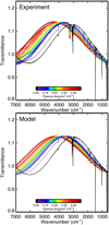 |
Fig. B.1 Benzene infrared spectra and modelling. Upper panel: Infrared transmittance spectra of a C6H6 ice film evolution as a function of 39.25MeV 56Fe10+ ion fluence. Lower Panel: Model spectra fitted to the data as a function of fluence. See text for model details. |
The expected column density of benzene ice can be estimated from the measured thickness using
 (B.2)
(B.2)
where NA, ρ, d, and  are the Avogadro number, the C6H6 ice density, the film thickness, and the molar mass of benzene, respectively. The C6H6 ice density adopted is ρ = 0.77 g/cm3 from Hudson & Yarnall (2022). We note that ion irradiations of ice films can induce an amorphous compaction of ice structures when starting from amorphous and porous ice films that can affect the density and thus column-density estimates. Compaction, given the cross-sections for other ices at such dE/dx, occurs for fluences of a few 1011 ions/cm2. With the fluences presented in this study, in the present experiments, we are analysing an amorphous compact C6H6 ice phase. The very first fluence points can be affected by a compaction phase change and we therefore do not include the first fluence points in the analysis. If another density is adopted, the extracted yield can be adjusted proportionally to the inverse of the newly adopted value. The column-density evolution as estimated from equation B.2 is shown in Fig. B.3.
From the slope of the column density evolution with thickness, the derived sputtering yield is Ys ≈ 1.1 ± 0.3 × 10⁴ C6H6/ion.
From the integration of the evolution of the CH band centered at about 680 cm−1, and using the integrated absorption strength of 1.62 ± 0.1 × 10⁻¹⁷ cm/molecule from Hudson & Yarnall (2022), the column density evolution as estimated from this band is shown in Fig. B.3. This evolution is driven by the bulk benzene radiolysis, and the destruction cross section can be evaluated to σdes = 2.4 ± 0.2 × 10⁻¹³ cm2. This confirms a posteriori that  .
.
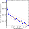 |
Fig. B.2 Column-density evolution as estimated from equation B.2 as a function of 39.25MeV 56Fe10+ ion fluence, with the thickness retrieved from the models presented in Fig. B.1. |
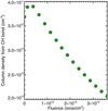 |
Fig. B.3 Column-density evolution as estimated from the integrated absorption of the 680 cm−1 benzene CH out of plane bond. |
Appendix C CH3CN sputtering yield determination
We proceed for the acetonitrile measurements analysis as for benzene, adopting an ice density of ρ = 0.78 g/cm3 from Hudson (2020) and optical constants {n,k} from Moore et al. (2010). This experiment was performed on a previously used ZnSe window coated with a thin carbon film and the refractive index of the substrate interface is higher than ZnSe, as can be seen from the increased amplitude of the interference fringes (Fig. C.1). We therefore constrained this index by minimisation with a constant that turns out to be close to n≈3.4. From the slope of the column density evolution with thickness (Fig. C.2), the derived sputtering yield is Ys ≈ 8.3 ± 3.4 × 10³ molecules/ion. From the integration of the evolution of the C≡N band centred at about 2250 cm−1, and using the integrated absorption strength of 2.3 ± 0.1 × 10⁻¹⁸ cm/molecule from D’Hendecourt & Allamandola (1986), the column density evolution as estimated from this band is shown in Fig. C.3. This evolution is driven by the bulk acetonitrile radiolysis, and the destruction cross section can be evaluated to σdes = 1.6 ± 0.2 × 10⁻¹³ cm2. This also confirms that for CH3CN, a posteriori,  .
.
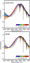 |
Fig. C.1 Acetonitrile infrared spectra and modelling. Upper panel: Infrared transmittance spectra of a CH3CN ice-film evolution as a function of 39.25MeV 56Fe10+ ion fluence. Lower Panel: Model spectra fitted to the data as a function of fluence. See text for model details. |
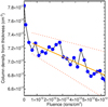 |
Fig. C.2 CH3CN column-density evolution as estimated from equation B.2 as a function of 39.25MeV 56Fe10+ ion fluence, with the thickness retrieved from the models presented in Fig. B.1. |
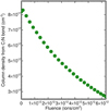 |
Fig. C.3 Column-density evolution as estimated from the integrated absorption of the 2250 cm−1 acetonitrile C≡N stretching bond. See text for detailed interpretation. |
References
- Augé, B., Been, T., Boduch, P., et al. 2018, Rev. Sci. Instrum., 89, 075105 [Google Scholar]
- Arakawa, I., Adachi, T., Hirayama, T., et al. 2000, Surf. Sci., 451, 136 [NASA ADS] [CrossRef] [Google Scholar]
- Bahr, D. A., & Baragiola, R. A. 2012, ApJ, 761, 36 [NASA ADS] [CrossRef] [Google Scholar]
- Baragiola, R. A., Vidal, R. A., Svendsen, W., et al. 2003, Nucl. Instrum. Methods Phys. Res. B, 209, 294 [Google Scholar]
- Bar-Nun, A., Herman, G., Rappaport, M. L., et al. 1985, Surf. Sci., 150, 143 [NASA ADS] [CrossRef] [Google Scholar]
- Basalgète, R., Ocaña, A. J., Féraud, G., et al. 2021, ApJ, 922, 213 [CrossRef] [Google Scholar]
- Bénit, J., Bibring, J.-P., Della-Negra, S., et al. 1987, Nucl. Instrum. Methods Phys. Res. B, 19/20, 838 [CrossRef] [Google Scholar]
- Bertin, M., Fayolle, E. C., Romanzin, C., et al. 2012, Phys. Chem. Chem. Phys., 14, 9929 [NASA ADS] [CrossRef] [Google Scholar]
- Bertin, M., Romanzin, C., Doronin, M., et al. 2016, ApJ, 817, L12 [NASA ADS] [CrossRef] [Google Scholar]
- Besenbacher, F., Bøttiger, J., Graversen, O., et al. 1981, Nucl. Instrum. Methods Phys. Res., 191, 221 [Google Scholar]
- Bisschoff, D., & Potgieter, M. S. 2016, Ap&SS, 361, 48 [NASA ADS] [CrossRef] [Google Scholar]
- Bohn, R. B., Sandford, S. A., Allamandola, L. J., et al. 1994, Icarus, 111, 151 [NASA ADS] [CrossRef] [Google Scholar]
- Børgesen, P., & Sørensen, H. 1982, Phys. Lett. A, 90, 319 [CrossRef] [Google Scholar]
- Bøttiger, J., Davies, J. A., L’ecuyer, J., Matsunami, N., & Ollerhead, R. 1980, Radiat. Effects, 49, 119 [CrossRef] [Google Scholar]
- Bouilloud, M., Fray, N., Bénilan, Y., et al. 2015, MNRAS, 451, 2145 [Google Scholar]
- Breuer, L., Meinerzhagen, F., Herder, M., et al. 2016, J. Vac. Sci. Technol. B 34 [Google Scholar]
- Bringa, E. M., & Johnson, R. E. 2003, Solid State Astrochem., 120, 357 [NASA ADS] [CrossRef] [Google Scholar]
- Brown, W. L., Augustyniak, W. M., Lanzerotti, L. J., et al. 1980, Phys. Rev. Lett., 45, 1632 [Google Scholar]
- Brown, W. L., Augustyniak, W. M., Simmons, E., et al. 1982, Nucl. Instrum. Methods Phys. Res. A, 198, 1 [CrossRef] [Google Scholar]
- Brown, W. L., Augustyniak, W. M., Marcantonio, K. J., et al. 1984, Nucl. Instrum. Methods Phys. Res. B, 1, 307 [NASA ADS] [CrossRef] [Google Scholar]
- Carrascosa, H., Cruz-Díaz, G. A., Muñoz Caro, G. M., et al. 2020, MNRAS, 493, 821 [CrossRef] [Google Scholar]
- Cervinka, C., & Fulem, M. 2017, J. Chem. Theory Comput., 13, 2840 [CrossRef] [Google Scholar]
- Chabot, M. 2016, A&A, 585, A15 [NASA ADS] [CrossRef] [EDP Sciences] [Google Scholar]
- Chen, Y.-J., Chuang, K.-J., Muñoz Caro, G. M., et al. 2014, ApJ, 781, 15 [Google Scholar]
- Chrisey, D. B., Boring, J. W., Phipps, J. A., et al. 1986, Nucl. Instrum. Methods Phys. Res. B, 13, 360 [NASA ADS] [CrossRef] [Google Scholar]
- Chrisey, D. B., Johnson, R. E., Phipps, J. A., et al. 1987, Icarus, 70, 111 [NASA ADS] [CrossRef] [Google Scholar]
- Cooper, B. H., & Tombrello, T. A. 1984, Radiat. Effects, 80, 203 [NASA ADS] [CrossRef] [Google Scholar]
- Dartois, E., Ding, J. J., de Barros, A. L. F., et al. 2013, A&A, 557, A97 [NASA ADS] [CrossRef] [EDP Sciences] [Google Scholar]
- Cruz-Diaz, G. A., Martín-Doménech, R., Muñoz Caro, G. M., et al. 2016, A&A, 592, A68 [NASA ADS] [CrossRef] [EDP Sciences] [Google Scholar]
- Cruz-Diaz, G. A., Martín-Doménech, R., Moreno, E., et al. 2018, MNRAS, 474, 3080 [NASA ADS] [CrossRef] [Google Scholar]
- Dartois, E., Chabot, M., Id Barkach, T., et al. 2019, A&A, 627, A55 [NASA ADS] [CrossRef] [EDP Sciences] [Google Scholar]
- Dartois, E., Chabot, M., Bacmann, A., et al. 2020, A&A, 634, A103 [NASA ADS] [CrossRef] [EDP Sciences] [Google Scholar]
- Dartois, E., Chabot, M., Koch, F., et al. 2022, A&A, 663, A25 [NASA ADS] [CrossRef] [EDP Sciences] [Google Scholar]
- Cummings, A. C., Stone, E. C., Heikkila, B. C., et al. 2016, ApJ, 831, 18 [CrossRef] [Google Scholar]
- Dartois, E., Augé, B., Boduch, P., et al. 2015, A&A, 576, A125 [NASA ADS] [CrossRef] [EDP Sciences] [Google Scholar]
- Dartois, E., Chabot, M., Id Barkach, T., et al. 2018, A&A, 618, A173 [NASA ADS] [CrossRef] [EDP Sciences] [Google Scholar]
- Dartois, E., Chabot, M., Id Barkach, T., et al. 2019, A&A, 627, A55 [NASA ADS] [CrossRef] [EDP Sciences] [Google Scholar]
- Dartois, E., Chabot, M., Id Barkach, T., et al. 2020, Nucl. Instrum. Methods Phys. Res. B, 485, 13 [Google Scholar]
- Dartois, E., Chabot, M., Id Barkach, T., et al. 2021, A&A, 647, A177 [EDP Sciences] [Google Scholar]
- D’Hendecourt, L.B., & Allamandola, L.J. 1986, A&AS, 64, 453 [Google Scholar]
- DeSimone, A. J., Crowell, V. D., Sherrill, C. D., et al. 2013, J. Chem. Phys., 139, 164702 [NASA ADS] [CrossRef] [Google Scholar]
- Dufour, C., & Toulemonde, M. 2016, Models for the Description of Track Formation, in Ion Beam Modification of Solids, eds. W. Wesch, & E. Wendler, Springer Series in Surface Sciences, 61 (Cham: Springer) [Google Scholar]
- Dupuy, R., Bertin, M., Féraud, G., et al. 2017a, A&A, 603, A61 [NASA ADS] [CrossRef] [EDP Sciences] [Google Scholar]
- Dupuy, R., Féraud, G., Bertin, M., et al. 2017b, A&A, 606, A9 [NASA ADS] [CrossRef] [EDP Sciences] [Google Scholar]
- Ellegaard, O., Schou, J., Sørensen, H., et al. 1986a, Surf. Sci., 167, 474 [NASA ADS] [CrossRef] [Google Scholar]
- Ellegaard, O., Schou, J., & Sørensen, H. 1986b, Nucl. Instrum. Methods Phys. Res. B, 13, 567 [NASA ADS] [CrossRef] [Google Scholar]
- Famá, M., Bahr, D. A., Teolis, B. D., et al. 2002, Nucl. Instrum. Methods Phys. Res. B, 193, 775 [CrossRef] [Google Scholar]
- Famá, M., Teolis, B. D., Bahr, D. A., et al. 2007, Phys. Rev. B, 75, 100101 [CrossRef] [Google Scholar]
- Fayolle, E. C., Bertin, M., Romanzin, C., et al. 2011, ApJ, 739, L36 [Google Scholar]
- Fayolle, E. C., Bertin, M., Romanzin, C., et al. 2013, A&A, 556, A122 [NASA ADS] [CrossRef] [EDP Sciences] [Google Scholar]
- Feistel, R., & Wagner, W. 2007, Geochim. Cosmochim. Acta, 71, 36 [NASA ADS] [CrossRef] [Google Scholar]
- Féraud, G., Bertin, M., Romanzin, C., et al. 2019, ACS Earth Space Chem., 3, 1135 [Google Scholar]
- Geballe, T. R., & Oka, T. 2010, ApJ, 709, L70 [Google Scholar]
- George, J. S., Lave, K. A., Wiedenbeck, M. E., et al. 2009, ApJ, 698, 1666 [Google Scholar]
- Gibbs, K. M., Brown, W. L., & Johnson, R. E. 1988, Phys. Rev. B, 38, 11001 [NASA ADS] [CrossRef] [Google Scholar]
- Ghosh, S., Avasthi, D. K., Som, T., et al. 2003, Nucl. Instrum. Methods Phys. Res. B, 212, 431 [NASA ADS] [CrossRef] [Google Scholar]
- Ghosh, S., Avasthi, D. K., Tripathi, et al. 2004, Nucl. Instrum. Methods Phys. Res. B, 219-220, 973 [CrossRef] [Google Scholar]
- Håkansson, P., & Sundqvist, B. U. R. 1989, Vacuum, 39, 339 [CrossRef] [Google Scholar]
- Haynes, W. M., Lide, D. R., & Bruno, T. J. 2016, CRC Handbook of Chemistry and Physics: A Ready-reference Book of Chemical and Physical Data, 20162017, 97th edn. (Boca Raton, Florida: CRC Press) [CrossRef] [Google Scholar]
- Hudson, R. L. 2020, Icarus, 338, 113548 [CrossRef] [Google Scholar]
- Hudson, R. L., & Moore, M. H. 2002, ApJ, 568, 1095 [NASA ADS] [CrossRef] [Google Scholar]
- Hudson, R. L., & Yarnall, Y. Y. 2022, Icarus, 377, 114899 [NASA ADS] [CrossRef] [Google Scholar]
- Indriolo, N., & McCall, B. J. 2012, ApJ, 745, 91 [NASA ADS] [CrossRef] [Google Scholar]
- Jamieson, C. S., & Kaiser, R. I. 2007, Chem. Phys. Lett., 440, 98 [NASA ADS] [CrossRef] [Google Scholar]
- Jóhannesson, G., Ruiz de Austri, R., Vincent, A.C., et al. 2016, ApJ, 824, 16 [CrossRef] [Google Scholar]
- Johnson, R. E., Pospieszalska, M., & Brown, W. L. 1991, Phys. Rev. B, 44, 7263 [NASA ADS] [CrossRef] [Google Scholar]
- Johnson, R. E., Carlson, R. W., Cassidy, T. A., & Fama, M. 2013, Sputtering of Ices, in eds. M. Gudipati, & J. Castillo-Rogez, The Science of Solar System Ices, Astrophysics and Space Science Library, 356 (New York, NY: Springer) [Google Scholar]
- Lähde, A., Raula, J., Malm, J., Kauppinen E.I., & Karppinen, M. 2009, Thermochim. Acta, 482, 17 [CrossRef] [Google Scholar]
- Lanzerotti, L. J., Brown, W. L., Augustyniak, W. M., et al. 1982, ApJ, 259, 920 [NASA ADS] [CrossRef] [Google Scholar]
- Lanzerotti, L. J., Brown, W. L., Marcantonio, K. J., et al. 1984, Nature, 312, 139 [NASA ADS] [CrossRef] [Google Scholar]
- Leger, A., Jura, M., & Omont, A. 1985, A&A, 144, 147 [Google Scholar]
- Lepoire, D. J., Cooper B.H., Melcher C.L., & Tombrello T.A. 1983, Radiolysis Effects, 71, 245 [NASA ADS] [CrossRef] [Google Scholar]
- Martín-Doménech, R., Manzano-Santamaría, J., Muñoz Caro, G. M., et al. 2015, A&A, 584, A14 [NASA ADS] [CrossRef] [EDP Sciences] [Google Scholar]
- Martín-Doménech, R., Cruz-Díaz, G. A., & Muñoz Caro, G. M. 2018, MNRAS, 473, 2575 [CrossRef] [Google Scholar]
- Martínez-Herrera, M., Campos, M., Torres, L. A., & Rojas, A. 2015, Ther- mochim. Acta, 622, 72 [CrossRef] [Google Scholar]
- McCall, B. J., Huneycutt, A. J., Saykally, R. J., et al. 2003, Nature, 422, 500 [CrossRef] [Google Scholar]
- Mejía, C., Bender, M., Severin, D., et al. 2015, Nucl. Instrum. Methods Phys. Res. B, 365, 477 [Google Scholar]
- Melcher, C. L., Lepoire, D. J., Cooper, B. H., et al. 1982, Geophys. Res. Lett., 9, 1151 [NASA ADS] [CrossRef] [Google Scholar]
- Moore, M. H., Ferrante, R. F., Moore, W. J., et al. 2010, ApJS, 191, 96 [NASA ADS] [CrossRef] [Google Scholar]
- Muñoz Caro, G. M., Jiménez-Escobar, A., Martín-Gago, J. Á., et al. 2010, A&A, 522, A108 [NASA ADS] [CrossRef] [EDP Sciences] [Google Scholar]
- Neufeld, D. A., & Wolfire, M. G. 2017, ApJ, 845, 163 [Google Scholar]
- de Nolfo, G. A., Moskalenko, I. V., Binns, W. R., et al. 2006, Adv. Space Res., 38, 1558 [Google Scholar]
- Öberg, K. I., Fuchs, G. W., Awad, Z., et al. 2007, ApJ, 662, L23 [Google Scholar]
- Öberg, K. I., Linnartz, H., Visser, R., et al. 2009, ApJ, 693, 1209 [CrossRef] [Google Scholar]
- Oja, V., & Suuberg, E. M. 1998, J. Chem. Eng. Data, 43, 486 [CrossRef] [Google Scholar]
- Oka, T., Geballe, T. R., Goto, M., et al. 2019, ApJ, 883, 54 [Google Scholar]
- O’Shaughnessy, D.J., Boring, J.W., Phipps, J.A., et al. 1986, Nucl. Instrum. Methods Phys. Res. B, 13, 304 [CrossRef] [Google Scholar]
- Pirronello, V., Strazzulla, G., Foti, G., et al. 1981, A&A, 96, 267 [NASA ADS] [Google Scholar]
- Prasad, S. S., & Tarafdar, S. P. 1983, ApJ, 267, 603 [Google Scholar]
- Querry M.R. 1987, Chemical Research, Development Engineering Center, Aberdeen, CRDEC-CR-88009 [Google Scholar]
- Raut, U., & Baragiola, R. A. 2013, ApJ, 772, 53 [Google Scholar]
- Rocard, F., Benit, J., Bibring, J. P., & Meuneir, R. 1986, Radia Effects, 99, 97 [NASA ADS] [CrossRef] [Google Scholar]
- Rothard, H., Domaracka, A., Boduch, P., et al. 2017, J. Phys. B, 50, 062001 [NASA ADS] [CrossRef] [Google Scholar]
- Reimann, C. T., Boring, J. W., Johnson, R. E., et al. 1984a, Appl. Surf. Sci., 147, 227 [NASA ADS] [CrossRef] [Google Scholar]
- Reimann, C. T., Johnson, R. E., & Brown, W. L. 1984b, Phys. Rev. Lett., 53, 600 [Google Scholar]
- Růžička, K., Fulem, M., & Cervinka, C. 2014, J. Chem. Thermodyn., 68, 40 [CrossRef] [Google Scholar]
- Ruehl, G., Harman, S. E., Árnadóttir, L., & Campbell, C. T. 2021, ACS Catal., 12, 156 [Google Scholar]
- Sandford, S. A., Bernstein, M. P., Allamandola, L. J., et al. 2001, ApJ, 548, 836 [NASA ADS] [CrossRef] [Google Scholar]
- Satorre, M. Á., Domingo, M., Millán, C., et al. 2008, Planet. Space Sci., 56, 1748 [Google Scholar]
- Satorre, M. Á., Luna, R., Millán, C., et al. 2018, Astrophys. Space Sci. Libr., 51 [NASA ADS] [CrossRef] [Google Scholar]
- Schou, J. 1987, Nucl. Instrum. Methods Phys. Res. B, 27, 188 [NASA ADS] [CrossRef] [Google Scholar]
- Schou, J. 2002, J. Nucl. Sci. Technol., 39, 4, 354 [NASA ADS] [CrossRef] [Google Scholar]
- Schou, J., & Pedrys, R. 2001, J. Geophys. Res., 106, 33309 [Google Scholar]
- Schou, J., Ellegaard, O., Sørensen, H., Pedrys, R. 1988, Nucl. Instrum. Methods Phys. Res. B, 33, 808 [CrossRef] [Google Scholar]
- Schriver-Mazzuoli, L., Chaabouni, H., & Schriver, A. 2003, J. Mol. Struct., 644, 151 [NASA ADS] [CrossRef] [Google Scholar]
- Seiberling, L. E., Meins, C. K., Cooper B.M., et al. 1982, Nucl. Instrum. Methods, 198, 17 [Google Scholar]
- Seperuelo Duarte, E., Boduch, P., Rothard, H., et al. 2009, A&A, 502, 599 [NASA ADS] [CrossRef] [EDP Sciences] [Google Scholar]
- Seperuelo Duarte, E., Domaracka, A., Boduch, P., et al. 2010, A&A, 512, A71 [NASA ADS] [CrossRef] [EDP Sciences] [Google Scholar]
- Shakeel, H., Wei, H., Pomeroy, J. M. 2018, J. Chem. Thermodyn., 118, 127 [CrossRef] [Google Scholar]
- Shen, C. J., Greenberg, J. M., Schutte, W. A., & van Dishoeck, E. F. 2004, A&A, 415, 203 [NASA ADS] [CrossRef] [EDP Sciences] [Google Scholar]
- Shi, M., Baragiola, R. A., Grosjean, D. E., et al. 1995, J. Geophys. Res., 100, 26387 [NASA ADS] [CrossRef] [Google Scholar]
- Sigmund, P. 1987, Nucl. Instrum. Methods Phys. Res. B, 27, 1 [NASA ADS] [CrossRef] [Google Scholar]
- Sigmund, P. 1995, Phys. Rev. A, 56, 3781 [Google Scholar]
- Smirnova, N. N., Bykova, T. A., Van Durme, K., & Van Mele, B. 2006, J. Chem. Thermodyn., 38, 879 [CrossRef] [Google Scholar]
- Souers, P. C., Briggs, C. K., Pyper, J. W., & Taugawa, R. T., 1977, UCRL-52226 [Google Scholar]
- Stenum, B., Schou, J., Ellegaard, O., et al. 1991a, Phys. Rev. Lett., 67, 2842 [NASA ADS] [CrossRef] [Google Scholar]
- Stenum, B., Ellegaard, O., Schou, J., et al. 1991b, Nucl. Instrum. Methods Phys. Res. B, 58, 399 [NASA ADS] [CrossRef] [Google Scholar]
- Stephenson, R. M., & Malanowski, S. 1987, Handbook of the Thermodynamics of Organic Compounds [CrossRef] [Google Scholar]
- Swanepoel, R. 1983, J. Phys. E Sci. Instrum., 16, 1214 [NASA ADS] [CrossRef] [Google Scholar]
- Torrisi, L., Coffa, S., Foti, G., & Strazzulla, G. 1986, Radiat. Effects, 100, 61 [NASA ADS] [CrossRef] [Google Scholar]
- Wang, J. Z., Seo, E. S., Anraku, K., et al. 2002, ApJ, 564, 244 [Google Scholar]
- Webber, W. R., & Yushak, S. M. 1983, ApJ, 275, 391 [Google Scholar]
- Westley, M. S., Baragiola, R. A., Johnson, R. E., et al. 1995, Nature, 373, 405 [NASA ADS] [CrossRef] [Google Scholar]
- Yuan, C., & Yates, J. T. 2013, J. Chem. Phys., 138, 154303 [NASA ADS] [CrossRef] [Google Scholar]
- Zhen, J., & Linnartz, H. 2014, MNRAS, 437, 3190 [NASA ADS] [CrossRef] [Google Scholar]
- Ziegler, J. F., Ziegler, M. D., & Biersack, J. P. 2010, Nucl. Instrum. Methods Phys. Res. B, 268, 1818 [Google Scholar]

All Tables
Sputtering yield prefactors and adopted low-temperature sublimation enthalpies for the considered species.
All Figures
|
Fig. 1 Influences of the different elements in processes associated with cosmic rays represented as fractional proportions on a log scale. Left: Galactic cosmic-ray abundance. Middle: relevance of the cosmic-ray elements in processes proportional to Z2, i.e. typically the radiolytic destruction of ices constituents. Right: relevance of the cosmic-ray elements in processes proportional to Z4, i.e. typically associated with the electronic sputtering mechanisms discussed in this article. |
| In the text | |
|
Fig. 2 Left: compendium of the sputtering yields Y obtained from the literature as a function of the electronic stopping power Se, to which are added our recent N2 measurement. The upper left dashed and dotted lines show the expected behaviour if the sputtering evolves linearly or quadratically, respectively, with the stopping power. The quadratic fit to each set of data for molecular systems and rare gases is over-plotted with dotted lines for comparison. Right: same data, assuming a quadratic dependency of the electronic sputtering yield on the stopping power, i.e. dividing the yield by Se2. Under this representation, a quadratic behaviour appears as a flat line, represented with dotted lines, and allows us to derive the sputtering yield prefactor |
| In the text | |
|
Fig. 3 Sputtering prefactor from Eq. (1) obtained from the fitting to the data presented in Fig. 2, reported as a function of the sublimation enthalpy of the considered species. A sputtering yield evolving quadratically with the stopping power has been adopted. There is a first-order correlation of |
| In the text | |
|
Fig. 4 Photodesorption rates from the literature reported as a function of enthalpy of sublimation. The variations in the absolute determination of the rate for various experiments are reported in Table 2. The right ordinate axis translates the rates into effective rates for a given ionisation rate ζ, assuming about 920 VUV photons cm−2 s−1 for an ionisation rate of ζ = 10−17 s−1. See text for details. |
| In the text | |
|
Fig. 5 Sputtering rate as a function of ionisation rate for H2O (blue), CO2 (red), and CO (green). The upper abscissa axis represents the approximate relation established between observed ionisation rate and the inverse of the visual extinction (e.g. Neufeld & Wolfire 2017). The arrow is shown to stress the fact that ices only appear above a visual extinction threshold (dependent on the particular dense cloud). This sets an upper limit to the maximum ionisation rate for dense cloud regions where they reside. The ionisation rate cannot be set arbitrarily high, even close to a strong source, as the cosmic rays spectrum is propagated (and therefore low energies attenuated) at least within a column density of matter corresponding to this minimum threshold AV. |
| In the text | |
|
Fig. 6 Ratio of cosmic rays to photodesorption rates calculated for a cosmic ray distribution leading to an ionisation rate of 3 × 10⁻¹⁷ s−1, and corresponding to about 2760 UV photons s−1 cm−2. See text for details. |
| In the text | |
|
Fig. A.1 Infrared spectra of the v4 vibrational mode for the CH4 ice experiment with 39.25 MeV 56Fe10+ ions. The inserted colour code gives the corresponding irradiation fluence. |
| In the text | |
|
Fig. A.2 CH4 sputtering yield determination. Left panel: CH4 column-density evolution measured with the v4 mode spectra as a function of 56Fe10+ ion fluence for a CH4 ice film deposited and measured at 10 K. Middle panel: Experimentally measured differential evolution of -dN/dF as a function of column density, to be compared to equation A.1. A fit of the equation to the data is shown as a black long-dashed line, and a fit not taking into account the finite depth of sputtering is shown with a short-dashed line. Right panel: Sputtering yield evolution as a function of column density; over-plotted are the infinite thickness yield (dashed lines) and adjusted exponential decay (long-dashed lines). See text for details. |
| In the text | |
|
Fig. B.1 Benzene infrared spectra and modelling. Upper panel: Infrared transmittance spectra of a C6H6 ice film evolution as a function of 39.25MeV 56Fe10+ ion fluence. Lower Panel: Model spectra fitted to the data as a function of fluence. See text for model details. |
| In the text | |
|
Fig. B.2 Column-density evolution as estimated from equation B.2 as a function of 39.25MeV 56Fe10+ ion fluence, with the thickness retrieved from the models presented in Fig. B.1. |
| In the text | |
|
Fig. B.3 Column-density evolution as estimated from the integrated absorption of the 680 cm−1 benzene CH out of plane bond. |
| In the text | |
|
Fig. C.1 Acetonitrile infrared spectra and modelling. Upper panel: Infrared transmittance spectra of a CH3CN ice-film evolution as a function of 39.25MeV 56Fe10+ ion fluence. Lower Panel: Model spectra fitted to the data as a function of fluence. See text for model details. |
| In the text | |
|
Fig. C.2 CH3CN column-density evolution as estimated from equation B.2 as a function of 39.25MeV 56Fe10+ ion fluence, with the thickness retrieved from the models presented in Fig. B.1. |
| In the text | |
|
Fig. C.3 Column-density evolution as estimated from the integrated absorption of the 2250 cm−1 acetonitrile C≡N stretching bond. See text for detailed interpretation. |
| In the text | |
Current usage metrics show cumulative count of Article Views (full-text article views including HTML views, PDF and ePub downloads, according to the available data) and Abstracts Views on Vision4Press platform.
Data correspond to usage on the plateform after 2015. The current usage metrics is available 48-96 hours after online publication and is updated daily on week days.
Initial download of the metrics may take a while.