| Issue |
A&A
Volume 647, March 2021
|
|
|---|---|---|
| Article Number | A177 | |
| Number of page(s) | 13 | |
| Section | Interstellar and circumstellar matter | |
| DOI | https://doi.org/10.1051/0004-6361/202039535 | |
| Published online | 30 March 2021 | |
Cosmic ray sputtering yield of interstellar ice mantles
CO and CO2 ice thickness dependence★
1
Institut des Sciences Moléculaires d’Orsay, UMR8214, CNRS, Université Paris-Saclay,
91405
Orsay,
France
e-mail: This email address is being protected from spambots. You need JavaScript enabled to view it.
2
Laboratoire de physique des deux infinis Irène Joliot-Curie, CNRS-IN2P3, Université Paris-Saclay,
91405
Orsay,
France
3
Centre de Recherche sur les Ions, les Matériaux et la Photonique, CIMAP-CIRIL-GANIL, Normandie Université, ENSICAEN, UNICAEN, CEA, CNRS,
14000
Caen,
France
4
Institut de planétologie et d’astrophysique de Grenoble, CNRS, Université Grenoble Alpes,
38000
Grenoble,
France
5
Department of Physics, Indian Institute of Technology,
Hauz Khas,
New Delhi
110016,
India
Received:
27
September
2020
Accepted:
22
January
2021
Abstract
Aims. Cosmic-ray-induced sputtering is one of the important desorption mechanisms at work in astrophysical environments. The chemical evolution observed in high-density regions, from dense clouds to protoplanetary disks, and the release of species condensed on dust grains, is one key parameter to be taken into account in interpretations of both observations and models.
Methods. This study is part of an ongoing systematic experimental determination of the parameters to consider in astrophysical cosmic ray sputtering. As was already done for water ice, we investigated the sputtering yield as a function of ice mantle thickness for the two next most abundant species of ice mantles, carbon monoxide and carbon dioxide, which were exposed to several ion beams to explore the dependence with deposited energy.
Results. These ice sputtering yields are constant for thick films. It decreases rapidly for thin ice films when reaching the impinging ion sputtering desorption depth. An ice mantle thickness dependence constraint can be implemented in the astrophysical modelling of the sputtering process, in particular close to the onset of ice mantle formation at low visual extinctions.
Key words: astrochemistry / cosmic rays / molecular processes / ISM: lines and bands / solid state: volatile / infrared: ISM
Part of the equipment used in this work has been financed by the French INSU-CNRS programme ‘Physique et Chimie du Milieu Interstellaire’ (PCMI).
© E. Dartois et al. 2021
 Open Access article, published by EDP Sciences, under the terms of the Creative Commons Attribution License (https://creativecommons.org/licenses/by/4.0), which permits unrestricted use, distribution, and reproduction in any medium, provided the original work is properly cited.
1 Introduction
In the dense and cold zones of the interstellar medium, dust grains are covered with volatile solids (the ice mantles), which are relatively protected from ambient radiation fields outside the cloud. However, cosmic radiation consisting of high-energy particles penetrates deeply into these clouds and induces complex chemistry through its direct interaction (radiolysis), or indirect interaction (production of a secondary vacuum ultraviolet-VUV- background radiation field by interaction with the gas, mainly molecular hydrogen) with dust grains. These cold and dense regions should in theory be considered as gas phase chemical ‘dead zones’ on time scales above the condensation (freeze-out) time of the whole gas phase on cold dust grains. The observation of a great diversity of species in the gas phase in these dense clouds thus implies the presence of mechanisms, not only of physico-chemical evolution, but also of desorption of the condensed species. Among these mechanisms are invoked chemical desorption (e. g. Yamamoto et al. 2019; Oba et al. 2018; Wakelam et al. 2017; Minissale et al. 2016a,b; Garrod et al. 2007), photodesorption by secondary VUV photons or X-rays (Westley et al. 1995; Öberg et al. 2009, 2011; Fayolle et al. 2011, 2013; Muñoz Caro et al. 2016, 2010; Cruz-Diaz et al. 2016, 2018; Fillion et al. 2014; Dupuy et al. 2017, 2018; Bertin et al. 2012, 2016), excursions in grain temperature (e.g. Bron et al. 2014), and sputtering in the electronic interaction regime by cosmic radiation (e.g. Seperuelo Duarte et al. 2009; Dartois et al. 2013, 2015; Boduch et al. 2015; Mejía et al. 2015; Rothard et al. 2017, and references therein). Once the efficiencies of these different processes have been quantitatively evaluated in the laboratory for a large number of systems, it is then possible to understand, through modelling, their absolute and relative impact on the chemistry of the interstellar medium.
The work presented in this paper is a continuation of a systematic study of the interstellar ice sputtering by cosmic radiation simulated in the laboratory. Of particular interest is the effect of the finite size of the interstellar ice mantle on the sputtering efficiency, which has been studied for H2O (Dartois et al. 2018), in the context here of two of the other major ice mantle components, CO and CO2. In Sect. 2, the experiments of irradiation by accelerated heavy ions is described. The model of evolution of the ices under the effect of this bombardment is described in Sect. 3. The fitting of the obtained data for CO and CO2 ices is presented in Sect. 4, leading to the determination of the finite sputtering depth for the considered ions. We then discuss the dependence of the sputtering depth on the stopping power and provide constraints for astrophysical models on the sputtering effective yield including finite size effects.
2 Experiments
Swift ion irradiation experiments were performed at the heavy-ion accelerator Grand Accélérateur National d’Ions Lourds (GANIL; Caen, France). Heavy ion projectiles were delivered on the IRRSUD beam line1. The IGLIAS (Irradiation de GLaces d’Intérêt AStrophysique) facility, a vacuum chamber (10−9 mbar under our experimental conditions) holding an infrared transmitting substrate that was cryocooled down to about 9 K, is coupled to the beam line. The ice films were produced by placing a cold window substrate in front of a deposition line. Carbon monoxide orcarbon dioxide films were condensed at 9 K on the window, from the vapour phase, and kept at this temperature during the irradiations. Details of the experimental setup are given in Augé et al. (2018). The ion flux, set between 107 and 109 ions cm−2 s−1 is monitored online using the current measured on the beam entrance slits defining the aperture. The irradiation is performed at normal incidence, whereas the infrared transmittance spectra are recorded simultaneously at 12o of incidence. Asweeping device allows for uniform and homogeneous ion irradiation over the target surface. The relation between the current at different slit apertures and the flux is calibrated before the experiments using a Faraday cup inserted in front of the sample chamber. The thin ice films deposited allow the ion beam to pass through the film with an almost constant energy loss per unit path length. A Bruker FTIR spectrometer (Vertex 70v) with a spectral resolution of 1 cm−1 was used to monitor the infrared film transmittance. The evolution of the infrared spectra was recorded as a function of the ion fluence. The projectiles used were 40Ca9+ at 38.4 MeV and 58Ni9+ at 33 MeV with an electronic stopping power, calculated using the SRIM package (Ziegler et al. 2010) for CO2 ice of Se = 1919.1 eV∕1015 CO2 molecules cm−2 and Se = 2487.8 eV∕1015 CO2 molecules cm−2, respectively. We also made use of additional experiments already presented in Seperuelo Duarte et al. (2009) for C18 O2 using a 46 MeV 58Ni11+ projectile, a measurement on a CO2 very thin film irradiated with a 630 MeV 132Xe21+ presented in Mejía et al. (2015), and a low-energy 100 keV proton irradiation experiment on CO2 from Raut & Baragiola (2013). For CO ice with projectiles of 40Ca9+ at 38.4 MeV, the Se = 1245.2 eV∕1015 CO molecules cm−2, and for 58 Ni9+ at 33 MeV, the Se = 1613.2 eV∕1015 CO molecules cm−2. We also made use of additional experiments already presented in Seperuelo Duarte et al. (2010) for CO using a 50 MeV 58 Ni 13+ projectile, and a low-energy 9 keV proton irradiation experiment from Schou & Pedrys (2001).
3 Model
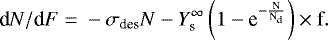
As discussed previously when modelling the evolution of water ice mantles (Dartois et al. 2015) and in the modelling of a sputtering crater in the N2 ice case of Dartois et al. (2020), the column density evolution of the ice molecules submitted to ion irradiation can be described, to first order and as a function of ion fluence (F) by a differential equation:
 (1)
(1)
N is the CO or CO2 column density. σdes is the ice effective radiolysis destruction cross-section (cm2).  is the semi-infinite (thick film) sputtering contribution in the electronic regime to the evolution of the ice column density, multiplied, to first order, by the relative concentration (f) of carbon monoxide or carbon dioxide molecules with respect to the total number of molecules and radicals in the ice film. f can be evaluated to first order by
  with X = CO2 or CO, neglecting the presence of radicals, carbon suboxides, and O2. In the case of CO2, one of the main products formed by irradiation is CO, and reaches about 20% of the ice at the top of its concentration. When the ice film is thin (column density N ≲ Nd; Nd being the semi-infinite‘sputtering depth’), the removal of molecules by sputtering follows a direct impact model, that is, all the molecules within the sputtering area defined by a sputtering ‘effective’ cylinder are removed from the surface. The apparent sputtering yield, as a function of thickness, is modelled to first order to estimate the corresponding sputtering depth by an exponential decay, leading to the 1 − e (−N∕Nd) correcting factor applied to
  . A schematic view of such a simplified cylinder approximation is shown in Fig. 1 of Dartois et al. (2018). The sputtering cylinder is defined by a radius rs (defining an effective sputtering cross section σs) and a height d (related to the measured sputtering depth). These parameters, reported in Table. 1, are calculated from the measurement of Nd and
  . These parameters also give access to the more or less prominent elongation of the sputtering cylinder, which is species- and deposited-energy-dependent. To monitor this elongation within the cylinder approximation one can calculate the so-called aspect-ratio parameter (height-to-diameter ratio of the cylinder in the semi-infinite ice film case). This model is a simplification. The reformation of the main species via the destruction of the daughter species is, for example, neglected as a second-order effect. The shape of the sputtering crater also influences the exact parametrisation, as shown in Dartois et al. (2020). An evolved model may be built when more precise data is acquired. Nevertheless, Nd is an efficient single parameter useful in estimating the sputtering depth in a column density equivalent.
The column densities of the molecules are followed experimentally in the infrared via the integral of the optical depth ( ) of a vibrational mode, taken over the band frequency range. The band strength value (A, in cm molecule−1) for a vibrational mode has to be considered. In the case of the 12 CO2 ν3 mode near 2342 cm−1, we adopted 7.6 × 10⁻¹⁷ cm molecule−1 (Bouilloud et al. 2015; Gerakines et al. 1995; D’Hendecourt & Allamandola 1986), although some measurements tend towards a higher value (~1.1 × 10⁻¹⁶ cm molecule−1; Gerakines & Hudson 2015). For the 12CO ν1 mode near 2342 cm−1, we adopted 1.1 × 10⁻¹⁷ cm molecule−1 (Bouilloud et al. 2015; Gerakines et al. 1995). The results are anchored to these adopted values and should be modified, if another reference value is favoured. Fits of Eq. (1) are shown in the middle panels of Figs. 1–6. Best parameters were retrieved with an amoeba method minimisation to find the minimum chi-square estimate on the model function. Only the experiments thick enough to sample the infinite thickness sputtering yield can be used. The fitted output parameters, namely σdes,
  , and Nd, are reported in Table 1, with the uncertainties being estimated at two times the reduced chi-square value obtained in the minimisation.
4 Results and discussion
4.1 Radiolysis, sputtering yield, and depth determination
The evolution of the infrared spectra (given in Appendix A) upon ion irradiation shows three stages that are much better understood when the data are plotted showing d N∕dF as a function of the column density, rather than the column density as a function of the fluence, evolving over several decades. We clearly see in Figs. 1–6 that the evolution of d N∕dF departs from the ideal model of Eq. (1), in particular at low fluence. At the beginning of irradiation, the ice film is restructuring with the first ions impinging the freshly deposited ice film. Therefore the molecular environment and phase is modified and/or compacted. The oscillator strength of the measured transitions in the infrared and/or the refractive index of the ice are slightly changing. As a consequence, the apparent dN∕dF evolution is rapid. At the considered stopping powers for the ions, this is stabilised after a fluence of a few 1011 ions cm−2, and the observed behaviour of dN∕dF better follows the expectation of the model. This early phase of the irradiation cannot be safely used to monitor the column density variations as both the molecule column density and the infrared band strength vary, leading to unpredictable changes, and they are discarded from the fits used to extract the model parameters (in the figures they are represented by light colours in the dN∕dF plots). Including these points in the fit leads to a misestimation of the radiolysis destruction cross-section. In the second evolution stage, the film can be considered semi-infinite with respect to the sputtering and d N∕dF evolves as a slope combining the radiolysis of the bulk and semi-infinite sputtering. In the later phase, the film becomes thin with respect to the sputtering’s semi-infinite sputtering depth (Nd) of individual ions. dN∕dF decreases accordingly with a linear and exponentially convolved behaviour.
In each experimental session, CO and CO2 films with several starting thicknesses (summarised in Table 1) were irradiated. This was done to estimate the reproducibility of the results, and also to check that the behaviour of the experimental results, particularly when reaching the thin film conditions, does not depend on the initial thickness. This can be seen in the middle panels of Figs. 1–6, in which the dN∕dF evolution is the same regardless of the initial film thickness within experimental uncertainties. It is important to state that it means that in these experiments the radiolysis (e.g. production of CO for CO2 films) does not accumulate enough to significantly affect the thin film’s behavioural evolution.
Experiments and results.
4.2 Experiments from the literature
4.2.1 CO2
We reanalysed the data from Seperuelo Duarte et al. (2009) on a C18 O2 ice film exposed to 58Ni11+ ions at 46 MeV. This is shown in Fig. 3. The right panel shows − d N∕dF as a function of the column density, with the previous fit with the parameters from Seperuelo Duarte et al. (2009) shown via a green dashed line, and the reanalysis with our current model via orange dashed lines. Our model includes an exponential decay at low column densities (long dashed orange lines). The dashed orange (straight) line shows what would be expected from thick film sputtering. As discussed above, the first points at low fluence, below about 1011 ions cm−2 were discarded from our fit, as they do not follow the theoretical expected − d N∕dF behaviour.
Mejía et al. (2015) reported a strong decrease of the sputtering yield for thin CO2 films exposed to 132Xe21+ ions at 630 MeV. Using the adjusted expected experimental yields for semi-infinite thick films, extrapolated to the stopping power of this experiment (Se = 5680 eV/1015 CO2 molecules cm−2), a crude estimate of the sputtering depth can be made. The thin film had a column density of Nthin = 6.8 × 1016 cm−2, and they report a measured sputtering yield of  . The sputtering yield at the same value of electronic stopping power for a semi-infinite thick ice film can be estimated from the thick film quadratic dependence, and we estimate it to be of the order of
  . From
  , one can estimate
  1017 cm−2.
To provide another point at low stopping power (Se = 46 eV/1015 CO2 molecules cm−2), we also include the sputtering of CO2 films induced by 100 keV H+ at 25K from Raut & Baragiola (2013). In this experiment, the authors measured a yield  . They did not measure the depth Nd. We can fix a range of variation by assuming upper and lower bounds limiting cases. For the lower bound, all sputtered molecules are assumed to come from the first layer. For the upper bound, they come from a depth thick as the yield. The mean value is taken as the cube root of the yield in monolayers, that is, a homogeneous 3D sputtering volume with no preferential extension along any axis. Assuming a density of 1.1 g cm−3 at 25K (Satorre et al. 2008) for the ice thickness and number of molecular layers, this leads to
  , providing an anchor point at low stopping power.
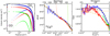 |
Fig. 1 Left panel: CO2 column density evolution measured with the anti-symmetric stretching mode (ν3) spectra as a function of 40Ca9+ ion fluence for CO2 ice films deposited with different initial thicknesses (shown with different colours) measured at 9 K. The radiolytically produced CO is also shown. Middle panel: experimentally measured differential evolution − d N∕d F as a function of column density, to be compared to Eq. (1). Fits of the equation to the data are shown as long-dashed lines (in black for the thickest film and orange for the intermediate thickness one) for the two thickest films, as well as fits not taking into account the finite depth of sputtering (dashed lines). No fit is attempted for the thinnest film. Right panel: sputtering yield evolution as a function of column density; over-plotted are the infinite thickness yield (dashed lines) and adjusted exponential decay (long-dashed lines). See text for details. The experiments are summarised in Table 1. |
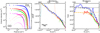 |
Fig. 2 Left panel: CO2 column density evolution measured with the anti-symmetric stretching mode (ν3) spectra as a function of 58Ni9+ ion fluence for CO2 ice films deposited with different initial thicknesses (shown with different colours) measured at 9 K. The radiolytically produced CO is also shown. Middle panel: experimentally measured differential evolution − d N∕d F as a function of column density, to be compared to Eq. (1). Fits of the equation to the data are shown as dashed lines for the two thickest films, as well as fits not taking into account the finite depth of sputtering (straight lines). Right panel: sputtering yield evolution as a function of column density; over-plotted are the infinite thickness yield (dashed lines) and adjusted exponential decay (long-dashed lines). See text for details. The experiments are summarised in Table 1. |
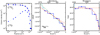 |
Fig. 3 Left panel: C18O2 ice experimental column densities for ion irradiation experiment (beam of 58Ni11+ at 46 MeV) discussed in Seperuelo Duarte et al. (2009). Middle panel: −dN∕dF calculated from the recorded data. The blue circles represent the data used in the fit, whereas the sky blue points are discarded as they represent the phase transition of the ice observed at the early irradiation stage (low fluence). The long, dashed orange line corresponds to the best-fit models using Eq. (1), and the dashed orange line to what would be expected from thick film behaviour. The dotted green line represents the fit using previously determined values from Seperuelo Duarte et al. (2009). Right panel: sputtering yield evolution and fitted contribution as a function of column density. |
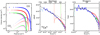 |
Fig. 4 Left panel: CO column density evolution at 9K as a function of at 33 MeV 58 Ni 9+ ion fluence for CO ice films deposited with different initial thickness (different colours). The radiolytically produced CO2 is shown. Middle panel: experimentally measured differential evolution −dN∕dF as a function of column density. The fit of Eq. (1) to the data for the thickest film is shown (long black dashed line), as well as a fit not taking into account the finite depth of sputtering (straight dashed line). Right panel: sputtering yield evolution and fitted contribution as a function of column density. |
4.2.2 CO
To provide another point at low stopping power (Se = 14 eV/1015 CO molecules cm−2), we also included the sputtering ofCO film induced by 9 keV H+ at 25K from Schou & Pedrys (2001). In this experiment, the authors measured a yield  . We again fixed its range of variation by assuming that all sputtered molecules come from the first layer for the lower bound, from a depth as thick as the yield for the upper bound, and the mean as the cube root of the yield in monolayers. Assuming a density of 0.8 g cm−3 at 10K (Loeffler et al. 2005; Bouilloud et al. 2015) for the ice thickness and the determination of the number of molecular layers, this leads to
  , providing an anchor point at low stopping power.
In this reanalysis of these previous literature data, CO and CO2 ice film temperatures are slightly higher than the one used in our experiments. The sputtering yield has been shown to be temperature-dependent, in particular in the case of H2O ice (e.g. Baragiola et al. 2003), with a higher yield when the temperature increases, Y = Y0 + Y1exp(−Ea/kT)), with an activation energy Ea that is related to the binding energy of the ice under consideration. For water ice it becomes significant above around 90 K. We thus expect that for CO2 ice, in the 9–30 K range considered here, the sputtering yield should be fairly constant. In the case of CO, the measured sputtering yield might be slightly higher than expected at the same temperature as the one we used in our measurements. However, as discussed above, the error bar set by our lack of knowledge on the corresponding sputtering depth for CO covers more than one order of magnitude, and we consider it most probably includes this uncertainty.
4.3 Relationship between sputtering depth and stopping power
The depth of sputtering obtained from the fit with the model of Eq. (1), along with the parameters of the fit, are reported in Table 1. Only the sufficiently thick films are fitted, as a sufficient number of points in the linear part of the curve is needed to retrieve the cross-section and the depth of sputtering simultaneously. The corresponding equivalent column density depth Nd is reported in Fig. 7 for CO2, and Fig. 8 for CO as a function of the stopping power. The best fit to the data as a function of the stopping power is  and
and  for CO2 and CO, respectively, that is, close to linear with the stopping power. Experiments and thermal spike models of the ion-track-induced phase transformation in insulators predict a dependence of the radius r of the phase change cross-section evolving as
  , where Se = dE∕dx is the deposited energy per unit path length (e.g. Lang et al. 2015; Toulemonde et al. 2000; Szenes 1997), with a threshold in
  to be determined. The measured semi-infinite (thick film) sputtering yield for ices (i.e. corresponding to the total volume) generally scales as the square of the ion electronic stopping power (
 , Rothard et al. 2017; Dartois et al. 2015; Mejía et al. 2015; Boduch et al. 2015). In the electronic sputtering regime considered in the present experiments, and as expected from the above cited dependences, it makes sense that the sputtering depth approximatively scales linearly with the stopping power and the aspect ratio scales with the square root of the stopping power.
An estimate of a sputtering cross-section can be inferred from our measurements with σs ≈ V∕d, where V is the volume occupied by  molecules and d the depth of sputtering.
  , where ml is the number of CO or CO2 molecules cm−2 in a monolayer (about 6.7 × 1014 cm−2 and 5.7 × 1014 cm−2, respectively,with the adopted ice densities). As is shown in Table 1, the sputtering radius rs would therefore be about 1.26 to 2.12 times larger than the radiolysis destruction radius rd in the case of the CO2 ice, and 2.03 to 2.36 for CO in the considered energy range (~0.5-1 MeV/u). The net radiolysis is the combined effect of the direct primary excitations and ionisations, the core of the energy deposition by the ion, and the so-called delta rays (energetic secondary electrons) travelling at much larger distances from the core; that is, several hundreds of nanometres at the considered energies in this work (e.g. Mozunder et al. 1968; Magee & Chatterjee 1980; Katz et al. 1990; Moribayashi 2014; Awad & Abu-Shady 2020). The effective radiolysis track radius that we calculate is lower than the sputtering one, which points towards a large fraction of the energy deposited in the core of the track. The scatter on the ratio of these radii is due to the lack of more precise data. It nevertheless allows to put a rough constraint on the estimate of Nd in the absence of additional depth measurements, with
  . If the rs∕rd ratio is high, a large amount of species come from the thermal sublimation of an ice spot less affected by radiolysis, and the fraction of ejected intact molecules is higher. The aspect ratio corresponding to these experiments evolves between about ten and twenty for CO2 and CO, whereas for water ice at a stopping power of Se ≈ 3.6 × 10³eV∕1015 H2 O molecules cm−2, we show that it is closer to one (Dartois et al. 2018). The depth of sputtering is much larger for CO and CO2 than for H2O at the same energy deposition, not only because their sublimation rate is higher, but also because they do not form OH bonds. For complex organic molecules embedded in ice mantles dominated by a CO or CO2 ice matrix, with the lack of OH bonding and the sputtering for trace species being driven by that of the matrix (in the astrophysical context), the co-desorption of complex organic molecules present in low proportions with respect to CO/CO2 cannot only be more efficient, but will thus arise from deeper layers.
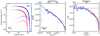 |
Fig. 5 Left panel: CO column density evolution at 9K as a function of at 33 MeV 58 Ni 9+ ion fluence for CO ice films deposited with different initial thickness (different colours). The radiolytically produced CO2 is shown. Middle panel: experimentally measured differential evolution −dN∕dF as a function of column density. The fit of Eq. (1) to the data for the thickest film is shown (long black dashed line), as well as a fit not taking into account the finite depth of sputtering (straight dashed line). Right panel: sputtering yield evolution and fitted contribution as a function of column density. |
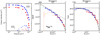 |
Fig. 6 Left: CO column density evolution at 9 K as a function of fluence for 50 MeV 58 Ni 13+ ion irradiation experiments (the blue one is discussed in Seperuelo Duarte et al. 2009) for ice films with different initial thicknesses (different colours). Radiolytically produced CO2 is shown. Middle panel: experimentally measured differential evolution −dN∕dF as a function of column density. The fit of Eq. (1) to the data for the thickest film is shown (long black dashed line), as well as a fit not taking into account the finite depth of sputtering (black dashed line). Right panel: sputtering yield evolution and fitted contribution as a function of column density. |
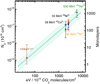 |
Fig. 7 Evolution of sputtering depth Nd as a functionof the stopping power for CO2 ice. The colour code for the points is the same as in Table 1. The best fit is given by
|

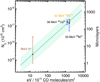 |
Fig. 8 Evolution of sputtering depth Nd as a function of the stopping power for CO ice. The colour code for the points is the same as in Table 1. The best fit is given by
|

4.4 Astrophysical modelling with finite size
If we integrate the sputtering yield over the distribution of galactic cosmic rays (GCR), the depth dependence of the yield can be parametrised in astrophysical models to provide an effective yield. Assuming the quadratic behaviour observed for many ices (e.g. Rothard et al. 2017; Dartois et al. 2015; Mejía et al. 2015; Boduch et al. 2015),
 (2)
(2)
where  is a pre-factor.
  is the stopping power in the electronic regime. For Se in units of eV∕1015molecules cm−2, we used
  for CO, 8.65 × 10⁻³ for CO2, and 5.93 × 10⁻³ for H2 O. The thickness-dependent sputtering yield in the electronic regime can be parametrised with the following prescription:
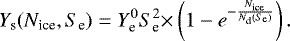 (3)
(3)
Nice is the ice column density, and Nd(Se) is the sputtering depth in column density equivalent, as determined in the previous section. The effective sputtering rate by cosmic rays can be calculated by integrating over their distribution in abundance and energies:
![Mathematical equation: \begin{eqnarray*} Y^{\textrm{eff}}_{\textrm{e}}(N_{\textrm{ice}}) = 2 {\times} 4\pi \sum_{Z} \int_{E_{\textrm{min}}}^{\infty} Y_{\textrm{s}} [N_{\textrm{ice}}, S_{\textrm{e}}(E,Z)] \frac{\textrm{d}N_{CR}}{\textrm{d}E}(E,Z) \textrm{d}E ,\end{eqnarray*}](/articles/aa/full_html/2021/03/aa39535-20/aa39535-20-eq29.png) (4)
(4)
where  is the effective sputtering rate for a given ice mantle thickness corresponding to a column density of Nice (or equivalently a number of monolayers),
 ![Mathematical equation: $ \frac{\textrm{d}N_{\textrm{CR}}}{\textrm{d}E}(E,Z) [\textrm{particles\,cm}^{-2}\,\textrm{s}^{-1}\,\textrm{sr}^{-1}/\textrm{(MeV/u)}]$](/articles/aa/full_html/2021/03/aa39535-20/aa39535-20-eq31.png) is the differential flux of the cosmic ray element of atomic number Z, with a cut-off in energy Emin set at 100 eV. Moving the cutoff from 10 eV to 1 keV does not change the results significantly. The differential flux for different Z follows the GCR observed relative abundances from Wang et al. (2002; H, He), de Nolfo et al. (2006; Li, Be), George et al. (2009; >Be), as explained in more detail in Dartois et al. (2013). The integration is performed up to Z = 28 corresponding to Ni; a significant drop in the cosmic abundance and thus also in contribution is observed above. The electronic stopping power Se is calculated using the SRIM code (Ziegler et al. 2010) as a function of atomic number Z and specific energy E (in MeV pernucleon). For the differential Galactic cosmic ray flux, we adopted the functional form given by Webber & Yushak (1983) for primary cosmic ray spectra using the leaky box model, also described in Shen et al. (2004):
is the differential flux of the cosmic ray element of atomic number Z, with a cut-off in energy Emin set at 100 eV. Moving the cutoff from 10 eV to 1 keV does not change the results significantly. The differential flux for different Z follows the GCR observed relative abundances from Wang et al. (2002; H, He), de Nolfo et al. (2006; Li, Be), George et al. (2009; >Be), as explained in more detail in Dartois et al. (2013). The integration is performed up to Z = 28 corresponding to Ni; a significant drop in the cosmic abundance and thus also in contribution is observed above. The electronic stopping power Se is calculated using the SRIM code (Ziegler et al. 2010) as a function of atomic number Z and specific energy E (in MeV pernucleon). For the differential Galactic cosmic ray flux, we adopted the functional form given by Webber & Yushak (1983) for primary cosmic ray spectra using the leaky box model, also described in Shen et al. (2004):
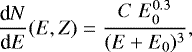 (5)
(5)
where C is a normalisation constant (=9.42 × 10⁴, Shen et al. 2004) and E0 a parameter influencing the low-energy component of the distribution. Under such parametrisation, the high-energy differential flux dependence goes asymptotically to a − 2.7 slope. The ionisation rate (ζ2) corresponding to the same distribution can be calculated, and it gives an observable comparison with astrophysical observations in various environments. The ionisation rates for E0 =200, 400, and 600 Mev u−1 correspond to ζ2 = 3.34 × 10⁻¹⁶s−1, 5.89 × 10⁻¹⁷ s−1, and 2.12 × 10⁻¹⁷ s−1, respectively. To show the dependence as a function of the number of layers, we set the value of C (E0 ≈ 520 Mev u−1) so that the ionisation rate corresponds to ζ2 = 3 × 10⁻¹⁷s−1, a typical value for the ionisation measured in dense clouds (Geballe & Oka 2010; Indriolo & McCall 2012; Neufeld, & Wolfire 2017; Oka et al. 2019).
The best fit to the thickness-dependent effective sputtering rates (molecules cm−2 s−1), integrated over the GCR distribution corresponding to ζ2 = 3 × 10⁻¹⁷s−1, can be adjusted with the following functional:
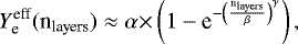 (6)
(6)
with α ~ 40.1, β ~ 75.8, γ ~ 0.69 for CO, α ~ 21.9, β ~ 56.3, γ ~ 0.60 for CO2, and α ~ 3.63, β ~ 3.25, γ ~ 0.57 for H2 O (plotted in brown, red, and blue in Fig. 9, respectively).
The typical thickness of ice mantles estimated from astronomical observations varies from a few to several hundreds of monolayers in dense clouds (Boogert et al. 2015 and references therein). In the dust particle size distribution, there might be signs of unusually large grain sizes or aggregates forming bigger particles, which is supported by the observations of scattering excess in spectral features or core shine effect (e.g. Jones et al. 2016; Steinacker et al. 2015; Dartois 2006). The ice mantle growth, and thus thickness, is, to first order, independent of the grain radius, but dependent on the temperature and density. In gas and grain astrochemical models, ice mantle thicknesses evolve with local conditions and time (e.g. Ruaud et al. 2016; Pauly & Garrod 2016). As the semi-infinite sputtering yield limit is reached rapidly with water ice, its effective sputtering, except at the border of clouds, should not vary significantly from the bulk, whereas for carbon dioxide and carbon monoxide, sputtering yield variations are expected when looking at the sputtering rate evolution displayed in Fig. 9.
To calculate the sputtering rates for different ionisation rates, we varied the E0 parameter in Eq. (5). It leads to a proportionality between the ionisation and sputtering rates (as in, e.g. Dartois et al. 2015; Faure et al. 2019). By doing so, one assumes that the energy spectra of all CR species are identical. For a CR spectrum with low energy particles impacting thick clouds containing the ice mantles, the stopping powers (different for each species) are differentially shaping the spectra during the propagation within the cloud (see Fig. 3 in Chabot 2016). To derive an estimate of the expected variations with respect to the simple proportionality between sputtering and ionisation rates, we propagated different initial CR spectra through clouds, as explained in Chabot (2016). We then calculated the ionisation rates and corresponding sputtering rates. In the worst case, the proportionality approximation overestimates the complete calculation by a factor 2. It occurs in the very dense parts of clouds (Av > 20) for initial CR spectra giving rise to high ionisation rates in the (unattenuated) external part of the cloud (ζ2 > 5 × 10⁻¹⁶ s−1). It is worth mentioning that magnetic fields may also affect such a proportionality between ionisation and sputtering rates. Indeed, proton and heavy particles do not have the same magnetic rigidity nor Larmor radius.
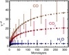 |
Fig. 9 Thickness-dependent effective sputtering rates (circles) in the electronic regime calculated for CO and CO2, for ζ2 = 3 × 10⁻¹⁷s−1, using the thickness dependence with stopping power derived in this article. The water ice behaviour is included for comparison, calculated using the single anchor point from Dartois et al. (2018). The functional Eq. (6) fitted to thedata is shown in dashed lines for each species. The typical absolute scale error bars are over-plotted. |
5 Conclusions
We measured the swift, heavy ion-induced CO and CO2 ice sputtering yield at ~10 K, and its dependence on the ice thickness. These measurements allow us to constrain the sputtering depth probed by the incident ion. Within the context of an ‘effective’ sputtering cylindrical shape to describe the sputtered molecule volume, the aspect ratio (height-to-diameter ratio of the cylinder in the semi-infinite ice film case) is higher than one, for the ion stopping powers considered in this study. The ejected molecules are arising from deeper layers than would be the case for a pure water ice mantle at the same deposited energies. The measured depth of desorption Nd scales with the ion electronic stopping power as ∝ Se 1.18 ± 0.19 (Se, deposited energy per unit path length) and ∝ Se 0.95 ± 0.17, for CO2 and CO, respectively. We thus experimentally measured a behaviour in agreement with what is expected from studies with swift heavy ions on insulators, as the phase transformations show a dependence of the radius r of the cross-sections evolving as  , and the ice’s total sputtering yields are generally proportional to the square of Se.
Following the trend measured, the depth of desorption evolves almost linearly with Se, and the aspect ratio dependence will thus scale as  , with α ~ 0.5. Astrophysical models should take into account this ice mantle’s thickness dependence constraints, in particular at the interface regions and onset of ice formation, that is, when ice is close to the measured extinction threshold. We provide a parametrisation based on our experiments, which can be used to describe the sputtering yield taking into account the finite nature of interstellar grains, ready for implementation in astrochemical models.
Acknowledgements
This work was supported by the Programme National ‘Physique et Chimie du Milieu Interstellaire’ (PCMI) of CNRS/INSU with INC/INP co-funded by CEA and CNES, and benefited from the facility developed during the ANR IGLIAS project, grant ANR-13-BS05- 0004, of the French Agence Nationale de la Recherche. Experiments performed at GANIL. We thank T. Madi, T. Been, J.-M. Ramillon, F. Ropars and P. Voivenel for their invaluable technical assistance. A.N.A. acknowledges funding from INSERM-INCA (Grant BIORAD) and Région Normandie fonds Européen de développement régional-FEDER Programmation 2014-2020. We would like to acknowledgethe anonymous referee for constructive comments that significantly improved the content of our article.
Appendix A Infrared spectra from the experiments
The baseline-corrected infrared optical depth spectra in the CO2 ν3 antisymmetric stretching mode and CO ν1 stretching mode region for the experiments reported in this work are displayed here for the different initial films’ thicknesses considered.
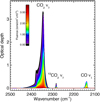 |
Fig. A.1 Infrared spectra for first CO2 ice experiment with 40Ca9+ at 38.4 MeVions. The inserted colour code gives the corresponding irradiation fluence. |
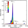 |
Fig. A.2 Infrared spectra for second CO2 ice experiment with 40Ca9+ at 38.4 MeVions. |
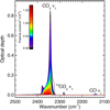 |
Fig. A.3 Infrared spectra for third CO2 ice experiment with 40Ca9+ at 38.4 MeVions. |
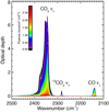 |
Fig. A.4 Infrared spectra for first CO2 ice experiment with 58Ni9+ at 33 MeV ions. We note that the spectra are saturated at the beginning of the experiment. These spectra were discarded from the analysis. |
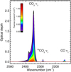 |
Fig. A.5 Infrared spectra for second CO2 ice experiment with 58Ni9+ at 33 MeV ions. |
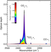 |
Fig. A.6 Infrared spectra for third CO2 ice experiment with 58Ni9+ at 33 MeV ions. |
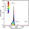 |
Fig. A.7 Infrared spectra for fourth CO2 ice experiment with 58Ni9+ at 33 MeV ions. |
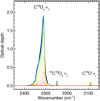 |
Fig. A.8 Infrared spectra for C18O2 ice experiments with 58Ni11+ at 46 MeV ions. |
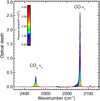 |
Fig. A.9 Infrared spectra for first CO ice experiment with 40Ca9+ at 38.4 MeV ions. |
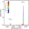 |
Fig. A.10 Infrared spectra for second CO ice experiment with 40Ca9+ at 38.4 MeVions. |
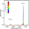 |
Fig. A.11 Infrared spectra for third CO ice experiment with 40Ca9+ at 38.4 MeVions. |
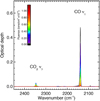 |
Fig. A.12 Infrared spectra for fourth CO ice experiment with 40Ca9+ at 38.4 MeVions. |
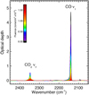 |
Fig. A.13 Infrared spectra for first CO ice experiment with 58Ni9+ at 33 MeV ions. We note that the spectra are saturated at the beginning of the experiment. These spectra were discarded from the analysis. |
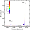 |
Fig. A.14 Infrared spectra for second CO ice experiment with 58Ni9+ at 33 MeV ions. |
References
- Augé, B., Been, T., Boduch, P., et al. 2018, Rev. Sci. Instrum., 89, 075105 [NASA ADS] [CrossRef] [Google Scholar]
- Awad, E. M., & Abu-Shady, M. 2020, Nucl. Instrum. Methods Phys. Res. B, 462, 1 [Google Scholar]
- Baragiola, R. A., Vidal, R. A., Svendsen, W., et al. 2003, Nucl. Instrum. Methods Phys. Res. B, 209, 294 [Google Scholar]
- Bertin, M., Fayolle, E. C., Romanzin, C., et al. 2012, Phys. Chem. Chem. Phys., 14, 9929 [Google Scholar]
- Bertin, M., Romanzin, C., Doronin, M., et al. 2016, ApJ, 817, L12 [Google Scholar]
- Boduch, P., Dartois, E., de Barros, A. L. F., et al. 2015, J. Phys. Conf. Ser., 629, 012008 [CrossRef] [Google Scholar]
- Boogert, A. C. A., Gerakines, P. A., & Whittet, D. C. B. 2015, ARA&A, 53, 541 [Google Scholar]
- Bouilloud, M., Fray, N., Bénilan, Y., et al. 2015, MNRAS, 451, 2145. [NASA ADS] [CrossRef] [Google Scholar]
- Bron, E., Le Bourlot, J., & Le Petit, F. 2014, A&A, 569, A100 [NASA ADS] [CrossRef] [EDP Sciences] [Google Scholar]
- Chabot, M. 2016, A&A, 585, A15 [NASA ADS] [CrossRef] [EDP Sciences] [Google Scholar]
- Cruz-Diaz, G. A., Martín-Doménech, R., Muñoz Caro, G. M., & Chen, Y.-J. 2016, A&A, 592, A68 [NASA ADS] [CrossRef] [EDP Sciences] [Google Scholar]
- Cruz-Diaz, G. A., Martín-Doménech, R., Moreno, E., Muñoz Caro, G. M., & Chen, Y.-J. 2018, MNRAS, 474, 3080 [NASA ADS] [CrossRef] [Google Scholar]
- Dartois, E. 2006, A&A, 445, 959 [NASA ADS] [CrossRef] [EDP Sciences] [Google Scholar]
- Dartois, E., Ding, J. J., de Barros, A. L. F., et al. 2013, A&A, 557, A97 [NASA ADS] [CrossRef] [EDP Sciences] [Google Scholar]
- Dartois, E., Augé, B., Rothard, H., et al. 2015, Nucl. Instrum. Methods Phys. Res. B, 365, 472 [NASA ADS] [CrossRef] [Google Scholar]
- Dartois, E., Chabot, M., Id Barkach, T., et al. 2018, A&A, 618, A173 [NASA ADS] [CrossRef] [EDP Sciences] [Google Scholar]
- Dartois, E., Chabot, M., Id Barkach, T., et al. 2020, Nucl. Instrum. Methods Phys. Res. B, 485, 13 [Google Scholar]
- D’Hendecourt, L. B., & Allamandola, L. J. 1986, A&AS, 64, 453 [NASA ADS] [Google Scholar]
- de Nolfo, G. A., Moskalenko, I. V., Binns, W. R., et al. 2006, Adv. Space Res., 38, 1558 [NASA ADS] [CrossRef] [Google Scholar]
- Dupuy, R., Bertin, M., Féraud, G., et al. 2017, A&A, 603, A61 [NASA ADS] [CrossRef] [EDP Sciences] [Google Scholar]
- Dupuy, R., Bertin, M., Féraud, G., et al. 2018, Nat. Astron., 2, 796 [Google Scholar]
- Faure, A., Hily-Blant, P., Rist, C., et al. 2019, MNRAS, 487, 3392 [CrossRef] [Google Scholar]
- Fayolle, E. C., Bertin, M., Romanzin, C., et al. 2011, ApJ, 739, L36 [NASA ADS] [CrossRef] [Google Scholar]
- Fayolle, E. C., Bertin, M., Romanzin, C., et al. 2013, A&A, 556, A122 [NASA ADS] [CrossRef] [EDP Sciences] [Google Scholar]
- Fillion, J.-H., Fayolle, E. C., Michaut, X., et al. 2014, Faraday Discuss., 168, 533 [Google Scholar]
- Garrod, R. T., Wakelam, V., & Herbst, E. 2007, A&A, 467, 1103 [NASA ADS] [CrossRef] [EDP Sciences] [Google Scholar]
- Geballe, T. R., & Oka, T. 2010, ApJ, 709, L70 [NASA ADS] [CrossRef] [Google Scholar]
- George, J. S., Lave, K. A., Wiedenbeck, M. E., et al. 2009, ApJ, 698, 1666 [Google Scholar]
- Gerakines, P. A., & Hudson, R. L. 2015, ApJ, 808, L40 [NASA ADS] [CrossRef] [Google Scholar]
- Gerakines, P. A., Schutte, W. A., Greenberg, J. M., & van Dishoeck, E. F. 1995, A&A, 296, 810 [NASA ADS] [Google Scholar]
- Indriolo, N., & McCall, B. J. 2012, ApJ, 745, 91 [NASA ADS] [CrossRef] [Google Scholar]
- Jones, A. P., Köhler, M., Ysard, N., et al. 2016, A&A, 588, A43 [NASA ADS] [CrossRef] [EDP Sciences] [Google Scholar]
- Katz, R., Loh K. S., Baling, L., Huang, G.-R. 1990, Radiat. Effects Defects Solids, 114, 15 [Google Scholar]
- Lang, M., Devanathan, R., Toulemonde, M., & Trautmann, C. 2015, Curr. Op. Solid State Mater. Sci., 19, 39 [Google Scholar]
- Loeffler, M. J., Baratta, G. A., Palumbo, M. E., et al. 2005, A&A, 435, 587 [NASA ADS] [CrossRef] [EDP Sciences] [MathSciNet] [Google Scholar]
- Magee, J. L., & Chatterjee, A. 1980, J. Phys. Chem., 84, 3529. [Google Scholar]
- Mejía, C., Bender, M., Severin, D., et al. 2015, Nucl. Instrum. Methods Phys. Res. B, 365, 477 [NASA ADS] [CrossRef] [Google Scholar]
- Minissale, M., Moudens, A., Baouche, S., et al. 2016a, MNRAS, 458, 2953 [NASA ADS] [CrossRef] [Google Scholar]
- Minissale, M., Dulieu, F., Cazaux, S., et al. 2016b, A&A, 585, A24 [NASA ADS] [CrossRef] [EDP Sciences] [Google Scholar]
- Moribayashi, K. 2014, Rad. Phys. Chem., 96, 211 [Google Scholar]
- Mozumder, A., Chatterjee, A., & Magee, J. L. 2016 Radiation Chemistry, (San Francisco: American Chemical Society), 27 [Google Scholar]
- Muñoz Caro, G. M., Jiménez-Escobar, A., Martín-Gago, J. Á., et al. 2010, A&A, 522, A108 [NASA ADS] [CrossRef] [EDP Sciences] [Google Scholar]
- Muñoz Caro, G. M., Chen, Y.-J., Aparicio, S., et al. 2016, A&A, 589, A19 [NASA ADS] [CrossRef] [EDP Sciences] [Google Scholar]
- Neufeld, D. A., & Wolfire, M. G. 2017, ApJ, 845, 163 [Google Scholar]
- Oba, Y., Tomaru, T., Lamberts, T., et al. 2018, Nat. Astron., 2, 228 [NASA ADS] [CrossRef] [Google Scholar]
- Öberg, K. I., Linnartz, H., Visser, R., & van Dishoeck, E. F. 2009, ApJ, 693, 1209 [NASA ADS] [CrossRef] [Google Scholar]
- Öberg, K. I., Boogert, A. C. A., Pontoppidan, K. M., et al. 2011, ApJ, 740, 109 [NASA ADS] [CrossRef] [Google Scholar]
- Oka, T., Geballe, T. R., Goto, M., et al. 2019, ApJ, 883, 54 [NASA ADS] [CrossRef] [Google Scholar]
- Pauly, T., & Garrod, R. T. 2016, ApJ, 817, 146 [NASA ADS] [CrossRef] [Google Scholar]
- Raut, U., & Baragiola, R. A. 2013, ApJ, 772, 53 [Google Scholar]
- Rothard, H., Domaracka, A., Boduch, P., et al. 2017, J. Phys. B At. Mol. Phys., 50, 062001 [Google Scholar]
- Ruaud, M., Wakelam, V., & Hersant, F. 2016, MNRAS, 459, 3756 [NASA ADS] [CrossRef] [Google Scholar]
- Satorre, M. Á., Domingo, M., Millán, C., et al. 2008, Planet. Space Sci., 56, 1748 [NASA ADS] [CrossRef] [Google Scholar]
- Schou, J., & Pedrys, R. 2001, J. Geophys. Res., 106, 33309 [Google Scholar]
- Seperuelo Duarte, E., Boduch, P., Rothard, H., et al. 2009, A&A, 502, 599 [NASA ADS] [CrossRef] [EDP Sciences] [Google Scholar]
- Seperuelo Duarte, E., Domaracka, A., Boduch, P., et al. 2010, A&A, 512, A71 [NASA ADS] [CrossRef] [EDP Sciences] [Google Scholar]
- Shen, C. J., Greenberg, J. M., Schutte, W. A., & van Dishoeck, E. F. 2004, A&A, 415, 203 [NASA ADS] [CrossRef] [EDP Sciences] [Google Scholar]
- Steinacker, J., Andersen, M., Thi, W.-F., et al. 2015, A&A, 582, A70 [NASA ADS] [CrossRef] [EDP Sciences] [Google Scholar]
- Szenes, G. 1997, Nucl. Instrum. Methods Phys. Res. B, 122, 530 [NASA ADS] [CrossRef] [Google Scholar]
- Toulemonde, M., Dufour, C., Meftah, A., & Paumier, E. 2000, Nucl. Instrum. Methods Phys. Res. B, 166, 903 [NASA ADS] [CrossRef] [Google Scholar]
- Wakelam, V., Loison, J.-C., Mereau, R., et al. 2017, Mol. Astrophys., 6, 22 [NASA ADS] [CrossRef] [EDP Sciences] [Google Scholar]
- Wang, J. Z., Seo, E. S., Anraku, K., et al. 2002, ApJ, 564, 244 [NASA ADS] [CrossRef] [Google Scholar]
- Webber, W. R., & Yushak, S. M. 1983, ApJ, 275, 391 [Google Scholar]
- Westley, M. S., Baragiola, R. A., Johnson, R. E., & Baratta, G. A. 1995, Nature, 373, 405 [NASA ADS] [CrossRef] [PubMed] [Google Scholar]
- Yamamoto, T., Miura, H., & Shalabiea, O. M. 2019, MNRAS, 490, 709 [Google Scholar]
- Ziegler, J. F., Ziegler, M. D., & Biersack, J. P. 2010, Nucl. Instrum. Methods Phys. Res. B, 268, 1818 [Google Scholar]
All Tables
All Figures
|
Fig. 1 Left panel: CO2 column density evolution measured with the anti-symmetric stretching mode (ν3) spectra as a function of 40Ca9+ ion fluence for CO2 ice films deposited with different initial thicknesses (shown with different colours) measured at 9 K. The radiolytically produced CO is also shown. Middle panel: experimentally measured differential evolution − d N∕d F as a function of column density, to be compared to Eq. (1). Fits of the equation to the data are shown as long-dashed lines (in black for the thickest film and orange for the intermediate thickness one) for the two thickest films, as well as fits not taking into account the finite depth of sputtering (dashed lines). No fit is attempted for the thinnest film. Right panel: sputtering yield evolution as a function of column density; over-plotted are the infinite thickness yield (dashed lines) and adjusted exponential decay (long-dashed lines). See text for details. The experiments are summarised in Table 1. |
| In the text | |
|
Fig. 2 Left panel: CO2 column density evolution measured with the anti-symmetric stretching mode (ν3) spectra as a function of 58Ni9+ ion fluence for CO2 ice films deposited with different initial thicknesses (shown with different colours) measured at 9 K. The radiolytically produced CO is also shown. Middle panel: experimentally measured differential evolution − d N∕d F as a function of column density, to be compared to Eq. (1). Fits of the equation to the data are shown as dashed lines for the two thickest films, as well as fits not taking into account the finite depth of sputtering (straight lines). Right panel: sputtering yield evolution as a function of column density; over-plotted are the infinite thickness yield (dashed lines) and adjusted exponential decay (long-dashed lines). See text for details. The experiments are summarised in Table 1. |
| In the text | |
|
Fig. 3 Left panel: C18O2 ice experimental column densities for ion irradiation experiment (beam of 58Ni11+ at 46 MeV) discussed in Seperuelo Duarte et al. (2009). Middle panel: −dN∕dF calculated from the recorded data. The blue circles represent the data used in the fit, whereas the sky blue points are discarded as they represent the phase transition of the ice observed at the early irradiation stage (low fluence). The long, dashed orange line corresponds to the best-fit models using Eq. (1), and the dashed orange line to what would be expected from thick film behaviour. The dotted green line represents the fit using previously determined values from Seperuelo Duarte et al. (2009). Right panel: sputtering yield evolution and fitted contribution as a function of column density. |
| In the text | |
|
Fig. 4 Left panel: CO column density evolution at 9K as a function of at 33 MeV 58 Ni 9+ ion fluence for CO ice films deposited with different initial thickness (different colours). The radiolytically produced CO2 is shown. Middle panel: experimentally measured differential evolution −dN∕dF as a function of column density. The fit of Eq. (1) to the data for the thickest film is shown (long black dashed line), as well as a fit not taking into account the finite depth of sputtering (straight dashed line). Right panel: sputtering yield evolution and fitted contribution as a function of column density. |
| In the text | |
|
Fig. 5 Left panel: CO column density evolution at 9K as a function of at 33 MeV 58 Ni 9+ ion fluence for CO ice films deposited with different initial thickness (different colours). The radiolytically produced CO2 is shown. Middle panel: experimentally measured differential evolution −dN∕dF as a function of column density. The fit of Eq. (1) to the data for the thickest film is shown (long black dashed line), as well as a fit not taking into account the finite depth of sputtering (straight dashed line). Right panel: sputtering yield evolution and fitted contribution as a function of column density. |
| In the text | |
|
Fig. 6 Left: CO column density evolution at 9 K as a function of fluence for 50 MeV 58 Ni 13+ ion irradiation experiments (the blue one is discussed in Seperuelo Duarte et al. 2009) for ice films with different initial thicknesses (different colours). Radiolytically produced CO2 is shown. Middle panel: experimentally measured differential evolution −dN∕dF as a function of column density. The fit of Eq. (1) to the data for the thickest film is shown (long black dashed line), as well as a fit not taking into account the finite depth of sputtering (black dashed line). Right panel: sputtering yield evolution and fitted contribution as a function of column density. |
| In the text | |
|
Fig. 7 Evolution of sputtering depth Nd as a functionof the stopping power for CO2 ice. The colour code for the points is the same as in Table 1. The best fit is given by
|
| In the text | |
|
Fig. 8 Evolution of sputtering depth Nd as a function of the stopping power for CO ice. The colour code for the points is the same as in Table 1. The best fit is given by
|
| In the text | |
|
Fig. 9 Thickness-dependent effective sputtering rates (circles) in the electronic regime calculated for CO and CO2, for ζ2 = 3 × 10⁻¹⁷s−1, using the thickness dependence with stopping power derived in this article. The water ice behaviour is included for comparison, calculated using the single anchor point from Dartois et al. (2018). The functional Eq. (6) fitted to thedata is shown in dashed lines for each species. The typical absolute scale error bars are over-plotted. |
| In the text | |
|
Fig. A.1 Infrared spectra for first CO2 ice experiment with 40Ca9+ at 38.4 MeVions. The inserted colour code gives the corresponding irradiation fluence. |
| In the text | |
|
Fig. A.2 Infrared spectra for second CO2 ice experiment with 40Ca9+ at 38.4 MeVions. |
| In the text | |
|
Fig. A.3 Infrared spectra for third CO2 ice experiment with 40Ca9+ at 38.4 MeVions. |
| In the text | |
|
Fig. A.4 Infrared spectra for first CO2 ice experiment with 58Ni9+ at 33 MeV ions. We note that the spectra are saturated at the beginning of the experiment. These spectra were discarded from the analysis. |
| In the text | |
|
Fig. A.5 Infrared spectra for second CO2 ice experiment with 58Ni9+ at 33 MeV ions. |
| In the text | |
|
Fig. A.6 Infrared spectra for third CO2 ice experiment with 58Ni9+ at 33 MeV ions. |
| In the text | |
|
Fig. A.7 Infrared spectra for fourth CO2 ice experiment with 58Ni9+ at 33 MeV ions. |
| In the text | |
|
Fig. A.8 Infrared spectra for C18O2 ice experiments with 58Ni11+ at 46 MeV ions. |
| In the text | |
|
Fig. A.9 Infrared spectra for first CO ice experiment with 40Ca9+ at 38.4 MeV ions. |
| In the text | |
|
Fig. A.10 Infrared spectra for second CO ice experiment with 40Ca9+ at 38.4 MeVions. |
| In the text | |
|
Fig. A.11 Infrared spectra for third CO ice experiment with 40Ca9+ at 38.4 MeVions. |
| In the text | |
|
Fig. A.12 Infrared spectra for fourth CO ice experiment with 40Ca9+ at 38.4 MeVions. |
| In the text | |
|
Fig. A.13 Infrared spectra for first CO ice experiment with 58Ni9+ at 33 MeV ions. We note that the spectra are saturated at the beginning of the experiment. These spectra were discarded from the analysis. |
| In the text | |
|
Fig. A.14 Infrared spectra for second CO ice experiment with 58Ni9+ at 33 MeV ions. |
| In the text | |
Current usage metrics show cumulative count of Article Views (full-text article views including HTML views, PDF and ePub downloads, according to the available data) and Abstracts Views on Vision4Press platform.
Data correspond to usage on the plateform after 2015. The current usage metrics is available 48-96 hours after online publication and is updated daily on week days.
Initial download of the metrics may take a while.