| Issue |
A&A
Volume 671, March 2023
|
|
|---|---|---|
| Article Number | A46 | |
| Number of page(s) | 19 | |
| Section | Galactic structure, stellar clusters and populations | |
| DOI | https://doi.org/10.1051/0004-6361/202245261 | |
| Published online | 06 March 2023 | |
New members of the Lupus I cloud based on Gaia astrometry
Physical and accretion properties from X-shooter spectra⋆
1
Dipartimento di Fisica e Astronomia, Universitá degli Studi di Padova, Vicolo dell’Osservatorio 3, 35122 Padova, Italy
e-mail: This email address is being protected from spambots. You need JavaScript enabled to view it.
2
INAF-Osservatorio Astronomico di Padova, vicolo dell’Osservatorio 5, 35122 Padova, Italy
3
INAF-Osservatorio Astronomico di Capodimonte, Via Moiariello 16, 80131 Napoli, Italy
4
INAF-Osservatorio Astrofisico di Catania, Via S. Sofia, 78, 95123 Catania, Italy
5
European Southern Observatory, Karl-Schwarzschild-Strasse 2, 85748 Garching bei München, Germany
6
Department of Physics, University of Rome Tor Vergata, Via della ricerca scientifica 1, 00133 Rome, Italy
7
Instituto de Física y Astronomía, Facultad de Ciencias, Universidad de Valparaíso, Av. Gran Bretaña 1111, Valparaíso, Chile
8
INAF-Rome Astronomical Observatory, Via di Frascati, 33, 00044 Monte Porzio Catone, Italy
9
Aix-Marseille Univ., CNRS, CNES, LAM, Marseille, France
Received:
21
October
2022
Accepted:
31
December
2022
Abstract
We characterize twelve young stellar objects (YSOs) located in the Lupus I region, spatially overlapping with the Upper Centaurus Lupus (UCL) sub-stellar association. The aim of this study is to understand whether the Lupus I cloud has more members than what has been claimed so far in the literature and gain a deeper insight into the global properties of the region. We selected our targets using the Gaia DR2 catalog based on their consistent kinematic properties with the Lupus I bona fide members. In our sample of twelve YSOs observed by X-shooter, we identified ten Lupus I members. We could not determine the membership status of two of our targets, namely Gaia DR2 6014269268967059840 and 2MASS J15361110-3444473 due to technical issues. We found out that four of our targets are accretors, among them, 2MASS J15551027-3455045, with a mass of ∼0.03 M⊙, is one of the least massive accretors in the Lupus complex identified to date. Several of our targets (including accretors) are formed in situ and off-cloud with respect to the main filaments of Lupus I; hence, our study may hint that there are diffused populations of M dwarfs around Lupus I main filaments. In this context, we would like to emphasize that our kinematic analysis with Gaia catalogs played a key role in identifying the new members of the Lupus I cloud.
Key words: accretion / accretion disks / stars: atmospheres / stars: activity / stars: chromospheres / stars: low-mass / stars: pre-main sequence
Based on observations collected at the European Southern Observatory at Paranal under program 105.20P9.001.
© The Authors 2023
 Open Access article, published by EDP Sciences, under the terms of the Creative Commons Attribution License (https://creativecommons.org/licenses/by/4.0), which permits unrestricted use, distribution, and reproduction in any medium, provided the original work is properly cited.
This article is published in open access under the Subscribe to Open model. This email address is being protected from spambots. You need JavaScript enabled to view it. to support open access publication.
1. Introduction
The observation of young stellar populations in nearby star-forming regions and comparison of their properties with more massive and distant ones is a key to understanding the impact of the environment on the star formation process and the properties of protoplanetary disks. The Lupus dark cloud complex is one of the main low-mass star-forming regions (SFRs) within 200 pc of the Sun. It consists of a loosely connected group of dark clouds and low-mass pre-main-sequence (PMS) stars. The complex hosts four active SFRs plus five other looser dark clouds with signs of moderate star-formation activity (Comerón 2008). Infrared (IR) and optical surveys (Evans et al. 2009; Rygl et al. 2012) have shown that objects in all evolutionary phases, from embedded Class I objects to evolved Class III stars, are found to be majorly concentrated in the Lupus I, II, and III clouds, with Lupus III being the richest in young stellar objects (YSOs). Different distances to the Lupus stellar subgroups have been claimed in the past from HIPPARCOS parallaxes and extinction star counts (Comerón 2008), but recent investigations based on Gaia DR2 showed that the vast majority of YSOs in all Lupus clouds are at a distance of ∼160 pc (see the appendix in Alcalá et al. 2019). Out of the three main clouds, Lupus III has been recognized as the most massive and active star-forming region in Lupus by far, with a great number of young, low-mass, and very-low mass stars (Comerón 2008), while Lupus I, II, and IV represent regions of low star-formation activity, with Lupus V and VI lacking star formation (Spezzi et al. 2011; Manara et al. 2018).
In this paper we investigate the Lupus I cloud. This cloud has fewer than thirty bona fide members, which from now on we refer to as Lupus I core members. The main motivation for selecting this cloud over the others with a low star-forming activity was the recent discovery of the star GQ Lup C (Alcalá et al. 2020; Lazzoni et al. 2020), which is located on the main filament.
This target was specifically selected by our team for discovering possible wide companions to SPHERE-GTO targets on Gaia DR2 with a high specific interest in the presence of planets, brown dwarfs, or spatially resolved circumstellar disks (Alcalá et al. 2020; Majidi et al. 2020). GQ Lup C was proven to be a strong accretor that had surprisingly escaped detection in previous IR and Hα surveys, suggesting the possibility that many YSOs in the region are yet to be discovered. This discovery hence motivated us to conduct a more extended search in Gaia DR2 to select new YSO candidates in the same region. In this work, we present the spectroscopic characterization of 12 YSOs in the Lupus I cloud.
The outline of this paper is as follows: in Sect. 2, we discuss the target selection criteria, as well as compiling a complete list of the bona fide Lupus I members, in addition to the observation and data reduction methods; in Sect. 3, we discuss the data analysis methods employed for analyzing the X-shooter spectra, the membership criteria, and accreting objects; in Sect. 4, we discuss the results of our analysis; in Sect. 5, we introduce additional qualities of our targets in Lupus I, present their spectral energy distributions (SEDs), and evaluate them as potential wide companion candidates; and, finally, Sect. 6 contains our conclusions.
2. Target selection, observations, and data reduction
2.1. Target selection
The Gaia astrometric catalog (Gaia Collaboration 2018) has recently been used to efficiently identify young clusters and associations within 1.5 kpc of the Sun (see Prisinzano et al. 2022 and references therein). We selected our sample of YSO candidates based on a statistical analysis using the Gaia DR2 catalog detailed in the following. As a first step, we identified the genuine population (core members) of Lupus I. These core members were gathered from the catalogs existing in the literature (Hughes et al. 1994; Merín et al. 2008; Mortier et al. 2011; Galli et al. 2013; Alcalá et al. 2014; Frasca et al. 2017; Benedettini et al. 2018; Dzib et al. 2018; Comerón et al. 2013; Galli et al. 2020) and are listed in Table 1. We calculated the membership probability of these targets to Upper Centaurus Lupus (UCL) with BANYAN Σ (Gagné et al. 2018a), which are also quoted in Table 1. It should be noted that the catalog does not evaluate the Lupus membership.
Lupus I core members known from the literature (measurement errors are displayed in parenthesis).
We then extracted the kinematic properties (i.e., parallaxes, ϖ, and proper motions μα* and μδ) of these core members from Gaia DR2 and constrained a range over these parameters (see Appendix B of Alcalá et al. 2020). Using this constrained range, we searched for the objects with similar kinematic properties to Lupus I core members in Gaia DR2 in a radius of three degrees from the center of the Lupus I cloud. At this stage, we found 247 objects. We placed these objects on a color-magnitude diagram (CMD) with main-sequence (MS) stars (Pecaut & Mamajek 2013), and we removed those that were close to the limiting magnitude of Gaia (with photometric errors preventing a reliable classification according to their position on the CMD) and we ended up with 186 targets. To generate this CMD, we used G magnitudes and Bp − Rp colors. This sample was then restricted to objects with a parallax within 5.5 to 7.5 mas (140–170 pc), within the ⟨ϖ⟩ ± 4 ⋅ σϖ parallax range of Lupus I core members; however, we kept both sources lying close to and far from the main filaments of Lupus I to be inclusive both with the kinematic properties and spatial location of the selected targets. We also excluded those objects that were too faint for X-shooter to observe (J > 15 mag) or older than typical YSOs in Lupus I (inconsistent with the Lupus I core members on our generated CMD).
Taking into account all these constraints, we identified 43 candidates as potential members of Lupus I. As shown in the CMD in Fig. 1, all of our eventual candidates lie above the MS stars identified by Pecaut & Mamajek (2013) and possess magnitudes and colors very similar to those of Lupus I members. Among these 43 objects, there are targets that (i) have never been recognized as potential members of Lupus I (17 objects); (ii) were introduced as candidate members of Lupus I according to their consistent kinematic and/or photometric properties, but need spectroscopic confirmation (23 objects); (iii) were known as members of Lupus I, but were poorly characterized in the literature and were never observed with X-shooter (3 objects). We chose to include all these categories of objects to be followed up by X-shooter, and the main reason for keeping the third category was that with X-shooter spectroscopy we can determine their radial velocity (RV) and projected radial velocity (v sin i) or explore their chromospheric and accretion properties in a more detailed fashion than previously done.
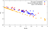 |
Fig. 1. CMD of all the potential members of Lupus I in our original sample of 43 objects (blue dots), with the MS stars (Pecaut & Mamajek 2013) (orange dots) and the Lupus I core members (red triangles) included in Table 1. |
Targets in this category are Sz 70 (Hughes et al. 1994), 2MASS J15383733-3422022 (Comerón et al. 2013), and 2MASS J15464664-3210006 (Eisner et al. 2007). Among the eight objects selected in Lupus I in the unbiased photometric survey by Comerón et al. (2013, see their Table 2), only three were selected by our criteria; these are the ones for which these authors provide stellar parameters, qualifying them as genuine YSOs. The other five were suspected to be foreground objects. Indeed, we confirmed that the astrometric parameters of the latter are out of range of our selection criteria.
As a final step, we cross-matched our full sample of 43 objects with the OmegaCAM Hα survey in Lupus (see Beccari 2018 for details of this survey), with only four being recognized as Hα emitters. This confirms that many potential YSOs may have escaped detection in Hα imaging surveys and motivated us to spectroscopically characterize our full sample, giving a high priority to the four OmegaCAM Hα emitters as potential strong accretors.
2.2. Observations
The observations were done with the X-shooter spectrograph (Vernet et al. 2011) at the VLT, within a filler program, and terminated at the end of the observing period, when only ∼28% of the proposed sample was observed. Hence, of the 43 proposed targets, only 12 were eventually observed that are fully characterized in this paper; these are listed in Table 2. The list of the targets that were not observed is reported in Appendix A. These 12 targets were selected by ESO staff from the list of our 43 proposed targets and include all of the Hα emitters. Although the observed sample is small, all of the 12 observed targets were confirmed to be YSOs whose physical and chromospheric/accretion properties are worth investigating. For two stars the OBs were not validated by ESO observing staff (due to not fulfilling some of our requirements). But the spectra are nevertheless useful for classification purposes and are used in this work.
Objects observed with X-shooter (measurement errors are displayed in parentheses).
X-shooter spectra are divided into three arms (Vernet et al. 2011): the UVB (λ ∼ 300–500 nm), VIS (λ ∼ 500–1050 nm), and NIR (λ ∼ 1000–2500 nm). We decided to observe all our targets with  ,
,  , and
, and  slit widths (for UVB, VIS, and NIR arms, respectively) for one or two cycles based on their J- band magnitudes. For our faintest objects with J > 14 mag, we considered two cycles of ABBA nodding mode. Among our observed targets, only 2MASS J15551027-3455045 belongs to this category, and due to its faintness, the final signal-to-noise ratio (S/N) of its spectra was lower than expected. The exposure time for each arm and the total execution time taking into account the overheads are reported for each target in Table 3. For our brightest target, TYC7335-550-1 with J = 9.65 mag, we decided that only one cycle of ABBA nodding would be sufficient for our scientific aims.
Observing log of the new candidate members of Lupus I.
Physical stellar parameters of the targets obtained with the ROTFIT code.
For some targets with a higher scientific significance to our program or because of their faintness, we decided to also observe telluric standard stars. Only a few of our targets (analyzed in this work) did not have a telluric star observation included in their observation block (OB); these are UCAC4 273-083363, 2MASS J15414827-3501458 (with J = 11.55 mag and 11.05 mag respectively), UCAC4 269-083981 (J = 10.72 mag), and Gaia DR2 6014269268967059840 (J = 13.64 mag), which had a lower scientific priority for our program – either they were not lying on the main filament, were not strong candidates for membership in Lupus I, were not Hα emitters, or were not faint enough for X-shooter to necessitate the observation of a telluric template. As we detail later, we also adopted a different approach to removing telluric lines for these objects. For the targets containing telluric observation in their OBs, the same nodding strategy as those of the targets was employed to minimize noise and cosmetics, with an airmass as close as possible to the targets’. The airmass and seeing reported in Table 3 are averaged over the exposure times for each arm.
2.3. Data reduction
The data used in this work have been reduced with the X-shooter pipeline XSHOO of version 2.3.12 and higher1, and hence they have been de-biased, flat-fielded, wavelength-calibrated, order-merged, extracted, sky-subtracted, and flux-calibrated. The result of this pipeline output is an ESO one-dimensional standard binary table and the two-dimensional ancillary files ready for scientific analysis. Flux calibration based on the photometric data available in the literature was done later, directly on the available spectra, along with the telluric removal process, which is not done for the distributed spectra reduced by the XSHOO pipeline.
We used the Image Reduction and Analysis Facility (IRAF, Tody 1986, 1993) to remove the telluric lines from the target spectra and to flux-calibrate them, as well as to derive the stellar parameters from the spectra, which we discuss in detail in the upcoming sections. Since the strategy for arranging our observation blocks did not include wide slit observations, the flux calibration of our targets totally relies on the photometric data available in the literature, which have been collected in various surveys (with the corresponding flux errors of e-16 W.m−2 for the UVB arm, e-16 W.m−2 for the VIS arm, and 2.5e-15 W.m−2 for the NIR arm). For some of our faint objects, we only had access to very limited photometric data and had to calibrate the UVB portion of the spectra in accordance with the available photometric data in the VIS range.
For the objects with observations of telluric standard stars, we removed the telluric lines and molecular bands using the IRAF task TELLURIC. For the three targets without telluric star observations in our sample, which namely are 2MASS J15414827-3501458, UCAC4 273-083363, and Gaia DR2 6014269268967059840, we used the TELFIT Python code. This code fits the telluric absorption spectrum in the observed spectra (Gullikson et al. 2014) using the LBLRTM code which models the line-by-line radiative transfer (Clough et al. 2005). Applying TELFIT, we corrected the spectra for oxygen and water molecular bands in the visible range (∼550–1000 nm), as well as for water, oxygen, and CO2 molecular bands in the NIR (∼1000–2500 nm) (for the details on the wavelength ranges where these molecular bands dominate the spectrum the reader is referred to Smette et al. 2015).
3. Data analysis
There are several immediate aims that we planned to fulfill through our program. With the X-shooter spectra, we can confirm the youth of the selected candidates through the presence of the Li I (6708 Å) absorption line, in addition to Hα emission, and other lines of the Balmer series as further hints. We also determine the spectral type (SpT) classification and the determination of stellar physical parameters such as effective temperature (Teff), luminosity (L), mass (M), and age. It is also possible that some of our candidates may belong to the Scorpius-Centaurus association (with an age of 10–18 Myr; UCL sub-association) rather than Lupus (1–2 Myr). We can single out these objects once we have fully characterized them. The disentanglement between the two associations would be useful for clarifying their relationship. Using spectral lines of the Balmer series, we will also measure the accretion luminosity (Lacc) and mass accretion rate (Ṁacc) of those objects that we qualify as accretors. In the following, we describe the methods used for achieving our immediate goals.
3.1. Spectroscopic analysis methods
3.1.1. Spectral typing and line equivalent widths
To obtain the SpTs of our objects, we first compared the spectrum obtained with X-shooter’s VIS arm with a library of visible spectra of already characterized stars and brown dwarfs formerly observed by X-shooter (Manara et al. 2013). For the quantitative spectral typing of the stars, we then calculated the spectral indices described in Riddick et al. (2007) based on the ratios of the average flux of molecular absorption bands within narrow wavelength regions, yielding in all cases an uncertainty of 0.5 subclasses. For TYC 7335-550-1 and UCAC4 269-083981, which are brighter than the rest of the targets and do not show clear molecular bands in their spectra suitable for measuring the Riddick indices, the SpT is instead estimated through the Teff obtained by the ROTFIT code (see Sect. 3.1.2). The results can be found in Table 7.
The EW of the atomic lines reported in Table 5 is measured by taking an average over (i) the direct integration of the line profiles between two marked pixels and (ii) fitting a Gaussian. The errors associated with these values thus report the difference between the measurements made with these methods. There are cases for which we could not detect the Li I line at 6708 Å. Hence, for these objects we only report an upper limit on the measurement of EWLi I. As suggested by Cayrel (1988), a three-sigma upper limit on the flux of the lithium line can be calculated as
 (1)
(1)
EWs of the relevant lines indicating the chromospheric and accretion tracers for our targets.
in which FWHM is the full width at half maximum, S/N is the signal-to-noise ratio, and the bin size (dx) can be fixed as 0.2 Å for the VIS arm. The values of these measurements are reported in Tables 5 and 6 for TYC7335-550-1.
EWs of the relevant lines indicating the chromospheric and accretion tracers for TYC 7335-550-1.
3.1.2. ROTFIT
We used ROTFIT as the basis of our analysis for assessing the stellar parameters of our targets. Using ROTFIT, we evaluated their RV, v sin i, and surface gravity (log g). The version of ROTFIT used for this purpose is the one designed for the optimal usage of the X-shooter spectra (Frasca et al. 2017). The stellar parameters obtained with ROTFIT can be found in Table 4. The fitting process with ROTFIT code was carried out within a veiling (the UV excess continuum that influences the entire photosphere of the star from UVB to NIR) range from 0 to 1. None of our objects showed significant veiling, and hence the veiling parameter for all our studied targets in this paper is equal to zero.
3.1.3. Physical parameters
We used the bolometric correction (BC) relation proposed by Pecaut & Mamajek (2013, 2016) for evaluating the luminosity in both V and J bands and the radius of candidates according to their observed parallaxes and magnitudes. This is possible because none of our targets show significant near-IR excess (Fig. 2) nor strong veiling (Sect. 3.1.2).
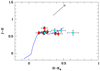 |
Fig. 2. J − H (mag) versus H − Ks (mag) diagram of all our targets. The red dots show the chromospherically dominant targets, the cyan dots are the accretors, and the blue line represents the colors of MS objects down to spectral type M9.5. The normal reddening vector, shown with the black arrow, corresponds to AV = 2 mag. The rightmost target is 2MASS J15361110-3444473 which is suspected to be a binary; hence, it might have color contribution from a second target. |
For the objects only resolved in Gaia DR2 catalog, the BC relationship introduced by the Gaia DR2 science team2 is used. In order to have a correct estimation of the luminosity, we have also taken into account the extinction of the objects, which was determined using the grid of X-shooter spectra of zero-extinction non-accreting T Tauri stars (Manara et al. 2013), as explained in Sect. 3.2 of Alcalá et al. (2014). It is evident from Fig. 2 that the targets have low extinction and little or no NIR excess, probably except for the rightmost point in the diagram, which corresponds to 2MASS J15361110-3444473. The relatively redder H − Ks color of this object in comparison with the others, may be due to the presence of an unresolved very late-type companion. This will be further discussed in Appendix C.
Once the Teff (from ROTFIT), luminosity, and radius of the targets are derived, their mass, age, and log g can be evaluated through various evolutionary tracks and isochrones available in the literature. The corresponding values of these parameters, which are reported in Table 7, are derived by the evolutionary models calculated by Baraffe et al. (2015). The Hertzsprung-Russel (HR) diagram of the Lupus I targets, including the previously known and the newly discovered members, is displayed Fig. 7. One of our targets, namely TYC 7335-550-1 is much brighter than the other stars investigated in the present work and falls outside the range covered by the Baraffe et al. (2015) models. Therefore, to derive its stellar parameters, we used MESA Isochrones and Stellar Tracks (MIST, Paxton et al. 2015; Choi et al. 2016; Dotter 2016). For modeling purposes, we assumed that all targets have solar metallicity (Baratella et al. 2020).
Physical stellar parameters of the targets.
Some of our objects display strong emission lines, which is a sign of noticeable chromospheric activity (see the EWs of some of the chromospheric activity indicators in Table 5) or magnetospheric accretion from a circumstellar disk. If the magnetic activity is relevant, the position of the star in the HR diagram can be significantly affected by photospheric starspots and by the changes in the internal structure induced by the magnetic fields (see Gangi et al. 2022 for interesting cases in the Taurus SFR). In this case, isochrones that do not take into account these effects (such as Baraffe et al. 2015) may lead to systematic effects in the estimate of mass and age. In particular, they may indicate an age half the real age of star (Asensio-Torres et al. 2019; Feiden 2016). This is crucial for our study, which also aims at determining the membership of the stars in Lupus I or UCL associations. Thus, in addition to MIST and the isochrones provided by Baraffe et al. (2015), we used other isochrones.
A set of evolutionary models that considers the magnetic activity of the stars is the Dartmouth magnetic isochrones (Feiden 2016), which we also used in this work to estimate the ages of all our targets. These isochrones were originally developed for estimating the age of the Upper Scorpius members (11 ± 2 Myr), almost coeval to the UCL (15 ± 3 Myr), and hence are quite useful to fulfill our scientific aims. In addition to Baraffe et al. (2015) and MIST models, we used both Dartmouth std and Dartmouth mag (Feiden 2016 and the references therein) models, as well as PARSEC + COLIBRI S37 (Bressan et al. 2012; Pastorelli et al. 2019, 2020). For all our targets, we obtained over-estimated ages using PARSEC + COLIBRI S37 isochrones totally inconsistent with the other isochrones; hence, to avoid confusion we do not report our results obtained with this isochrone. The results of age estimation with all the other isochrones are included in Table B.1. For all the models, we have assumed our targets have solar metallicity. For PARSEC models, extinction is also a free parameter that can be fixed and was thus set to the corresponding extinction of the targets reported in Table 7. We would like to point out that it is not straightforward to state which targets may have an underestimated age, particularly in the case of objects that are as young as the members of Lupus I and UCL considered in this work.
3.2. Lupus I membership criteria
According to the works previously done in the Lupus complex (Alcalá et al. 2014 and references therein), in addition to the kinematic properties expressed by the Gaia parallax and proper motions, membership criteria in this star-forming region are: (i) the presence of lithium in their atmospheres, which is the main signature of youth (despite the obviousness of this criterion, there are previously acknowledged members of the Lupus cloud that lack lithium; an example is represented by Sz 94 in the Lupus III cloud (Manara et al. 2013; Biazzo et al. 2017; Frasca et al. 2017; ii) an age consistent with the core members of the cloud; although the estimated age of the Lupus complex is ∼1–2 Myr, there are previously recognized members of the complex that exceed this age range (examples of such targets are AKC2006 18 and AKC2006 19 in Lupus I, or in Sect. 7.4 of Alcalá et al. 2014, although their apparent old age may be ascribed to disks seen edge-on that obscure the central objects making them subluminous on the HR diagram); and (iii) an RV consistent with the values of the genuine members of the Lupus I (Frasca et al. 2017). If an object does not match the membership criteria defined above, there are two possibilities. Either it is older than the UCL (age> 20 Myr), and we would hence identify it as field star; or, it has a consistent age with UCL (∼15 Myr), which would confirm its membership to this sub-cloud of the Scorpius-Centaurus stellar association. To this aim, we have used various isochrones to evaluate the age of our targets.
3.3. Accreting objects
There are several criteria for determining whether an object is actively accreting matter. Usually, an accreting object is characterized by strong emission lines, strong UV and NIR continuum excess emission, or structured line profiles (e.g., Manara et al. 2013). Here, to establish whether an object is an accretor, we used the criterion proposed by White & Basri (2003) that distinguishes the accreting and non-accreting objects based on the EW of their Hα emission versus SpT (Fig. 3). The method used in this paper for calculating the Lacc (accretion luminosity) and Ṁacc (mass accretion rate) of our targets involves measuring the line luminosity of the emission lines of the accreting targets and using the established relationships between the Lline (for each emission line) with Lacc (Alcalá et al. 2017). We quote the eventual accretion line luminosity that is obtained this way as log Lacc − line in Tables 8 and 9.
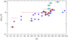 |
Fig. 3. |EWHα| versus SpT of our targets with the weak lined T Tauri stars studied by Manara et al. (2013, blue dots). The cyan dots represent accretors, and the red dots represent chromospherically dominant objects. The horizontal lines in red represent the thresholds that separate non-accreting and accreting objects considering their SpTs (White & Basri 2003). |
Accretion luminosity of the accretors derived from the line luminosities.
Accretion luminosity of TYC 7335-550-1 derived from its line luminosities.
The whole procedure that we carried out for this task can be summarized as follows: we corrected the spectra for telluric lines and flux-calibrated them, measured the flux at Earth of the emission lines by integrating their profile above the local continuum, corrected the flux for extinction, calculated the luminosity of each emission line by multiplying the flux at Earth for 4πd (adopting a distance d = 1000/ϖ pc, with ϖ in mas), and eventually took an average over all the values of log Lacc − line. We chose Hα, Hβ, and Hγ emission lines to measure the accretion luminosity of our targets. After deducing the log Lacc for each target, we obtained their Ṁacc accordingly (Alcalá et al. 2017). The results of our measurements are presented in Table 8.
Among all our targets, only TYC 7335-550-1 does not show Hydrogen emission lines above the continuum, and its Hα line is instead in absorption. For this target, we used ROTFIT to subtract the photospheric template in order to measure the flux of the emission components that fill the cores of Hydrogen and Ca II lines. This method has been successfully used to emphasize chromospheric emission or a moderate accretion whenever the photospheric flux is large and the emission is only detectable as a filling of the line core or an emission bump within the photospheric line wings that do not emerge above the continuum (e.g., Frasca et al. 2015, 2017, and references therein). The spectral subtraction allows us to recognize and measure the EW of the emission that fills in the Hα line (Fig. 4). Adopting the same method, we measured the fluxes of the H&K lines of the Ca II and in the cores of the three infrared lines of the Ca II IRT at λ = 849.8, 854.2, and 866.2 nm (Fig. 5). We were also able to separate the contribution of the Hϵ emission from the nearby Ca II H line.
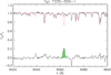 |
Fig. 4. X-shooter spectrum of TYC 7335-550-1 in Hα region, normalized to the local continuum (black solid line) along with the inactive photospheric template (red dotted line). The latter is produced by ROTFIT with the BT-Settl synthetic spectrum at the Teff and log g of this target that is degraded to the resolution of X-shooter, rotationally broadened, and wavelength-shifted according to the target RV. The difference target-template is displayed at the bottom of the box and emphasizes the Hα emission that fills in the line core (green hatched area), which has been integrated to obtain the Hα line flux. |
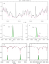 |
Fig. 5. X-shooter spectra of TYC 7335-550-1 in various wavelength portions. (a) X-shooter UVB spectrum of TYC 7335-550-1 in the Ca II H&K region (black solid line) along with the inactive photospheric template (red dotted line). (b) and (c) Residual (target-template) spectrum around the Ca II K and Ca II H lines, respectively. The hatched green areas mark the residual H and K emissions that have been integrated to obtain the EWs and fluxes. The purple-filled area relates to Hϵ. (d) and (e) Observed Ca II IRT line profiles (black solid lines) with the photospheric template overlaid with red dotted lines. The residual spectra are shown at the bottom of each panel shifted downward by 0.2 in relative flux units for clarity. |
4. Results
4.1. Stellar parameters and membership
The physical stellar parameters that we obtained from the spectral analysis and the HR diagram as described in Sects. 3.1.1 and 3.1.3 are reported in Table 7. The stellar parameters obtained with ROTFIT are presented in Table 4, where the membership probability was recalculated with the BANYAN Σ using the values of RVs measured with ROTFIT. Both Teff and log g found with ROTFIT are in good agreement with those derived from SpT and the HR diagram and reported in Table 7.
We note that, at the resolution of the X-shooter VIS spectra, the minimum value of v sin i that can be measured is 8 km s−1 (see, e.g., Frasca et al. 2017) and hence this value should be considered as an upper limit. With this knowledge, we can classify targets with v sin i < 8 km s−1 as slow rotators, and those with v sin i > 40 km s−1 as fast rotators. Moreover, the large RV range of the bona fide members of Lupus I (∼–5–12 km s−1, according to Table 1) prevents us from putting a strict constraint on the Lupus I membership of our targets (Fig. 6). The RVs of the Lupus I members confirmed in this work, however, are within a smaller range with respect to the previously confirmed core members of the same region, except for 2MASS J15361110-3444473, which may or may not be a Lupus I member.
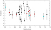 |
Fig. 6. RV of our accretors (cyan dots), chromospherically dominant targets (red dots), and the Lupus I core members (black dots). |
According to our full characterization, besides TYC 7335-550-1, which is a K4.5 type star, all the others have M spectral types. Three-quarters of our targets have spectral types between M4 and M6, which is in accordance with the previously identified members of the Lupus complex (Alcalá et al. 2014; Frasca et al. 2017; Krautter et al. 1997; Herczeg & Hillenbrand 2014; Comerón et al. 2013; Galli et al. 2020). The ages of these targets cover a large range of 0.7–11 Myr, with masses in the range of 0.02 to 1.1 M⊙ (as also indicated in Fig. 7).
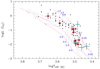 |
Fig. 7. log L⋆(L⊙) versus log Teff (K) diagram for all our targets (cyan and red dots represent accretors and non-accretors, respectively), together with the previously characterized Lupus members (black dots, Alcalá et al. 2019, subluminous objects are not plotted). Blue dashed lines represent evolutionary tracks of Baraffe et al. (2015) for stars with masses indicated by the number (in M⊙) next to the top or bottom of each track. The red lines indicate isochrones calculated with the same models at ages of 1, 3, 30 Myr and 10 Gyr, from the right to the left. |
As discussed in Sect. 2.1, Sz 70 and 2MASS J15383733-3422022 were partially known in the literature. The physical parameters that we report here for Sz 70 are in excellent agreement with the results of Hughes et al. (1994). For 2MASS J15383733-3422022, our results are again in good agreement with those reported by Comerón et al. (2013), but their difference emanates from the fact that Comerón et al. (2013) measured AV = 1.2 mag for 2MASS J15383733-3422022, which results in a discrepancy in luminosity, mass, and radius.
4.2. Equivalent widths
The EWs of several spectral lines are quoted in Table 5. The EWs of several spectral lines for TYC 7335-550-1 are separately reported in Table 6; as for this star the flux and EW measurements were performed by subtracting the photospheric spectrum.
We could not detect the Li I line in the spectra of some of our targets for various reasons, which can be (i) solely due to the low S/N of their spectra; (ii) based on the simulations conducted by Constantino et al. (2021), for initially lithium-rich stars we know that slow rotators could deplete their lithium (also considering their SpT) at early ages (< 10 Myr), while fast rotators tend to retain their lithium; (iii) a combination of the low S/N and fast rotation (which may be especially true for Gaia DR2 6014269268967059840), which would further complicate the issues associated with Li I detection; (iv) a complex relationship between the accretion processes, early angular momentum evolution, and possibly planet formation for young stars (∼5 Myr) that yet needs to be fully explored (Bouvier et al. 2016; v) a lack of obvious relationship between the rotation of YSOs and the lithium depletion process (Binks et al. 2022). The non-detection of Li I in the spectra of some objects has been reported as a three-sigma upper limit on the flux of the lithium line, which is a sensitive enough threshold for separating them from objects containing lithium.
4.3. Evolutionary status of the targets
The main properties and final status of all our targets are summarized in Table 10. Based on all the criteria discussed in Sect. 3.2, we confirm that all our objects are YSOs, with ages of < 11 Myr.
Overall status checklist for our targets.
The targets 2MASS J15414827-3501458 and UCAC4 273-083363 do not show the presence of the lithium line in the spectra, but their effective temperature is compatible with the possible presence of a large amount of Li depletion for fully convective pre-main-sequence stars (Bildsten et al. 1997). Lithium depletion was investigated in several star-forming regions, such as certain subgroups of Orion (Palla et al. 2007; Sacco et al. 2007), but also in Lupus I and III (see, e.g., Biazzo et al. 2017 and references therein). Due to their very young age (< 4 Myr), we therefore classify 2MASS J15414827-3501458 and UCAC4 273-083363 as Lupus I members. Newly discovered members of Lupus I in this work are 2MASS J15523574-3344288, 2MASS J16011870-3437332, and Gaia DR2 6010590577947703936.
There are also two objects analyzed in this work that we could not identify either as a member of Lupus I or UCL. These are 2MASS J15361110-3444473, whose spectrum indicates an unresolved binary star of spectral types M5.5 (VIS arm) and M8 (NIR arm), and we could not detect lithium in its spectrum (see Appendix C for more details on the analysis of this target). However, we would like to emphasize that 2MASS J15361110-3444473 is an accreting source that has consistent kinematic and physical properties with the genuine members of Lupus I, hence, there is a possibility that this target also qualifies as a new member of Lupus I. The other object is Gaia DR2 6014269268967059840, for which we acquired a spectrum with a poor S/N (see Sect. 2 for details on the observation conditions of this target). The poor S/N of its UVB spectrum hindered us from carrying out any measurements on its Hβ and Hγ lines in emission (as reported in Table 5), which also leads to evaluating its accretion properties only according to its Hα emission line (as reported in Table 8). Therefore, the non-detection of lithium in its spectrum can be purely due the poor S/N in the VIS arm, and we neither approve nor rule out the possibility of this target being a member of Lupus I.
We hence confirm that all our targets are YSOs, with Hydrogen lines in emission above the continuum. Therefore, this investigation suggests that although only four of our targets were retrieved as Hα emitters in the OmegaCAM survey (flagged in Table 2), it is likely that our entire sample of 43 candidate YSOs could include Hα emitters or objects with filled Hα profiles, which can only be confirmed by a high- or mid-resolution spectroscopic study or in deep X-ray surveys.
As a further investigation to strengthen our argument, we cross-matched all of the Lupus I core members included in Table 1 with the OmegaCAM survey. Except for three objects, they were all retrieved in the survey as Hα emitters. These three exceptional core members are RXJ1529.7-3628 (which was out of the field of view of the survey), RX J1539.7-3450B, and Sz 68/HT Lup C, for which only one object was resolved in the survey. Combining this result with the results of this paper, we emphasize the necessity of observing all our sample to characterize all the members of Lupus I that have escaped the Hα surveys.
4.4. Accretion versus chromospheric–dominated objects
We realized that four of our targets in the current sample are accretors. We measured the Lacc of these targets, in addition to our chromospherically-dominant objects (Table 8 and Table 9). The measured Lacc for all our targets are displayed in Fig. 8. In the same figure, we have included the limits suggested by Manara et al. (2017) for objects with Teff > 4000 K and Teff < 4000 K, below which the chromospheric activity of targets is dominant. All four of our accretors exceed this limit for targets with Teff < 4000 K, confirming that they are accretion-dominated. The rest of our targets within the same effective temperature range are below this threshold, which makes them chromospheric-dominated objects, as expected. 2MASS J15523574-3344288, however, lies exactly on the threshold between these two regimes, which is consistent with its significant Hα emission. We also emphasize that this target was retrieved in the OmegaCAM survey as an Hα emitter.
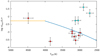 |
Fig. 8. Log ⟨Lacc/L*⟩ versus Teff for all our targets. The cyan dots represent accretors and the red dots represent chromospherically dominant targets. The lines indicate the limit below which the chromospheric activity for a star is dominant (Manara et al. 2017), for two regimes of stars with Teff ≤ 4000 K (the diagonal blue line) and those with Teff ≥ 4000 K (the horizontal orange line). |
Figure 9 shows the Ṁacc versus M* for the four accretors in our sample in comparison with the Lupus members. Among the four accretors, 2MASS J15551027-3455045 is the least massive target and has a very high mass accretion rate in comparison with Lupus members of similar mass. This target also stands above the double power-law relationship between Ṁacc and M* established by Vorobyov & Basu (2009), based on modeling self-regulated accretion by gravitational torques in self-gravitating disks. As concluded by Alcalá et al. (2017), only the strongest accretors stand above this model. Our three other accretors have values of mass accretion rates typical of Lupus accretors.
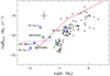 |
Fig. 9. Log Macc(M⊙/yr) versus log M*(M⊙) for the four accretors in our sample (cyan dots), together with the previously identified members of the Lupus (black dots). The blue crossed squares represent the sub-stellar accreting companions detected at wide orbits by Zhou et al. (2014) around GQ Tau, GSC 06214 00210, and DH Tau as labeled. 2MASS J15551027-3455045, GQ Lup c and 2MASS J16085953-3856275 are also labeled. 2MASS J15523574-3344288 is labeled as a red dot. The continuous red line indicates the double power-law prediction of Vorobyov & Basu (2009), while the magenta dashed line shows the prediction of the disk fragmentation model by Stamatellos & Herczeg (2015). |
Finally, it is worth noting that three of our accretors (Sz 70, 2MASS J15361110-3444473, and 2MASS J16011870-3437332) have WHα(10%) > 270 km s−1 (see Table 5), which is expected from accreting stars. Our chromospherically-dominant targets have much narrower Hα profiles.
5. Discussion
In this work, we analyzed 12 objects observed by X-shooter out of our original sample of 43 proposed new candidate members of Lupus I. We confirm that all 12 of these objects are YSOs, and ten out of 12 are members of Lupus I. We could not determine the membership of two of our targets, namely 2MASS J15361110-3444473 and Gaia DR2 6014269268967059840, as explained in the previous section. We could not fully measure the accretion properties of Gaia DR2 6014269268967059840, and hence our analysis in this regard for this specific target is not reliable. 2MASS J15361110-3444473, on the other hand, is a rather (intrinsic) faint object to be followed up by any available spectrographs, but perhaps it can be followed up with ALMA to understand whether it is surrounded by a disk. Although recognized to be older with respect to Lupus I members (9 Myr), it may still be strongly accreting matter, consistently with the members of γ Vel with ages of ∼10 Myr (Frasca et al. 2015). One of the interesting targets discussed in this work is TYC 7335-550-1, a lithium-rich K-type star with Hα in absorption and without IR excess. We would like to emphasize that YSOs with these particular characteristics would never appear in Hα imaging surveys such as OmegaCAM, although one of their main aims is to identify the members of young star forming regions. All the above points considered, we have fully characterized ten members of Lupus I in this work.
In the following, we discuss other qualities of our targets. To this aim, we carried out further investigations, which are mainly based on the data available in the literature in connection with the targets analyzed in this work.
5.1. Spectral energy distributions and circumstellar disks
For all our objects, we also investigated whether there are hints of continuum flux excess suggestive of circumstellar disks. To this aim, we extracted their SEDs from literature which are collectively exhibited in Figs. 10 and 11. For this work, we only concentrate on the morphology and trends of the SEDs of our targets, as well as their near- to mid-infrared photometric data (published by 2MASS and WISE surveys). To generate the SEDs, we used the following WISE filters: W1 (3.4 microns), W2 (4.6 microns), W3 (12 microns), W4 (22 microns). In a parallel paper (Majidi et al. in prep.), we study the variability of these stars and model their disks.
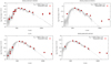 |
Fig. 10. BT-Settl models (in gray) with the photometric data (red dots) for our accretors. |
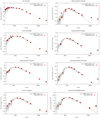 |
Fig. 11. BT-Settl models (in gray) with the photometric data (red dots) for our chromospherically dominant targets. |
The photometric data for all four accretors significantly deviate from their BT-Settl spectral model (based on their Teff, log g, and zero metallicity) in W3 and W4 filters (with the average flux errors of 5e-17 W.m−2 and 1.7e-16 W.m−2, respectively). This trend can be observed for our less massive, stronger accretors 2MASS J15551027-3455045 and 2MASS J15361110-3444473 in all four WISE filters (W1, W2, W3, and W4). According to Sicilia-Aguilar et al. (2014), the morphology of the SEDs of all our four accretors in addition to 2MASS J15523574-3344288 is compatible with objects surrounded by full disks (Table 11). This is further confirmed by the disk categorization of Bredall et al. (2020) based on Ks − W3 and Ks − W4 magnitudes for Lupus dippers, Lupus YSOs, Upper Scorpius, and Taurus members. Hence, also according to Bredall et al. (2020), all four of our accretors, in addition to 2MASS J15523574-3344288, are surrounded by a full disk. We note, however, that the “valley” around W3 in the SED of 2MASS J15361110-3444473 is typical of those seen in transitional disks.
Disk categorization of all our targets, in addition to their reddest colors available in the 2MASS and WISE catalogs.
For the rest of our targets, we have two categories of circumstellar disks based on the morphology of their SEDs further approved by their Ks − W3 and Ks − W4 magnitudes: (i) evolved disks, which are characterized by only W4 excess with respect to the theoretical BT-Settl model, and are evident in the SEDs of 2MASS J15383733-3422022, Gaia DR2 6010590577947703936, and Gaia DR2 6014269268967059840 (Fig. 11); (ii) debris disks, which are characterized by little to no mid-infrared excess, evident in the SEDs of TYC 7335-550-1, UCAC4 269-083981, 2MASS J15414827-3501458, and UCAC4 273-083363 (Fig. 11).
5.2. High accretion in the low-mass regime
Deriving Ṁacc for the lowest mass accretors is relevant for the studies of disk evolution. There is growing evidence of a change in the slope of the M⋆–Ṁacc relationship for YSOs with ages of 2–3 Myr at M⋆ < 0.2 M⊙ (Manara et al. 2017 and Alcalá et al. 2017, and see Fig. 9). Such a break could be related to a faster disk evolution at the low-masses (e.g. Vorobyov & Basu 2009). To verify this, the Ṁacc–M⋆ relationship needs to be sampled at much lower M⋆ and Ṁacc values than has been done so far.
Our target 2MASS J15551027-3455045 is one of the lowest mass accretors in Lupus (see Fig. 7). With M⋆ = 0.02 M⊙, 2MASS J16085953-3856275 is the accretor with comparable mass reported in the previous Lupus studies (Alcalá et al. 2017, 2019). Considering the very low mass of this YSO, its accretion rate Ṁacc ∼10−11 M⊙ yr−1 (Alcalá et al. 2019) is relatively high. Yet, the Ṁacc value for 2MASS J15551027-3455045 is about an order of magnitude higher (see Fig. 9); hence, it is one of strongest accretors in Lupus in the mass range of 0.02–0.03 M⊙, that is, close to the planetary mass regime. From the modeling of a shock at the surface of a planetary-mass object, Aoyama et al. (2021) predicted much higher Lacc values than what the scaling Lacc–Lline relations for stars predict. The relationships by these authors would yield an even higher Ṁacc value, almost an order of magnitude higher than our estimate. This object falls above the model prediction by Vorobyov & Basu (2009), in contrast with the idea of faster disk evolution at very low masses. However, statistics are still rather poor at this mass regime for a firm conclusion.
Other very low-mass YSOs, companions to T Tauri stars, have been found to exhibit similar, or even higher rates of mass accretion (Betti et al. 2022; Zhou et al. 2014, see Fig. 9). To explain the very high levels of accretion observed in such sub-stellar and planetary-mass companions, Stamatellos & Herczeg (2015) modeled the accretion onto very low-mass objects that formed by the fragmentation of the disk around the hosting star. During the early evolution the individual disks of sub-stellar companions, including those at the planetary-mass regime, accrete additional material from the gas-rich parent disk, and, hence, their disks are more massive and their accretion rates are higher than if they were formed in isolation. Therefore, these very low-mass objects have disk masses and accretion rates that are independent of the mass of the central object and are higher than expected from the scaling relation Ṁacc ∝  of more massive YSOs. These models predict that Ṁacc is independent of M⋆.
Using Gaia DR3, we investigated whether 2MASS J15551027-3455045 might be a wide companion of another star, but it is an isolated object. Hence, the high mass-accretion rate cannot be explained in terms of the Stamatellos & Herczeg (2015) scenario. Due to its intrinsic faintness, 2MASS J15551027-3455045 would be an interesting target to be followed up by CUBES, which is a next-generation spectrograph suitable for investigating fainter, low-mass, accreting YSOs (Alcalá et al. 2022).
5.3. Possible wide companions
While studying the kinematic properties of the targets, we also noticed that a few of our targets and core members of the Lupus I share similar kinematic properties, and can be considered as wide companion candidates. These wide companion candidates are presented in Tables 12 and 13, divided into two categories of candidates studied in this work and the Lupus I core members. In order to understand whether two objects with similar kinematic properties are gravitationally bound, we calculated their total velocity difference (Δv) and compared it with the maximum total velocity difference (Δvmax) as a function of projected separation between the two binary components, suggested by Andrews et al. (2017). If Δv exceeds Δvmax, we do not expect the two targets to be gravitationally bound. It should be noted, however, that the theoretical maximum velocity difference modeled by Andrews et al. (2017) is only for binaries of total mass 10 M⊙ in circular orbits. We summarize our results on identifying wide companions candidates in the Lupus I cloud as follows.
Kinematic properties of the Lupus I members from this work (measurement errors are displayed in parentheses).
Core members of Lupus I sharing similar kinematic properties (measurement errors are displayed in parentheses).
5.3.1. Sz 70 and Sz 71
As the GQ Lup triple system (Alcalá et al. 2020), Sz 70 and Sz 71 (GW Lup) are located on the main filament of Lupus I. Sz 70 lies at a separation of 32.32 arcsec from GW Lup, and in between these objects lies the X-ray source [KWS97] Lupus I 37 (Krautter et al. 1997) at a separation of 24.23 arcsec from Sz 70. We conducted a chance projection study in Alcalá et al. (2020, Appendix E), which was focused on understanding how probable it is to find a field object around a genuine member of Lupus I, lying on the same filament where GQ Lup stellar system and Sz 70/Sz 71 are located. The linear density of this filament is 0.0024 objects/arcsecond, or an average object separation of 418 arcsec, which is 13 times the observed separation between Sz 70 and Sz 71. As exhibited in Fig. 12, Sz 70 and Sz 71 do not qualify as gravitationally bound stars, but we would like to emphasize that the test proposed by Andrews et al. (2017) is only valid for gravitationally bound binaries, and not systems of higher multiplicities (if this is the case for this stellar system). Hence, we would consider this case as a wide companion candidate that cannot be confirmed or ruled out according to the available information.
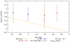 |
Fig. 12. Log-log plot of total velocity difference Δv (km s−1) versus projected separation (au) for the wide companion candidates analyzed in this work, in addition to the genuine wide companions GQ Lup and GQ Lup C. Δvmax (km s−1) (orange line) indicates the maximum total velocity difference that bound binaries with a total mass equal to 10 M⊙ in circular orbits can possess (Andrews et al. 2017). Each point is marked as one of the wide companion candidates involved. For the detailed information (see Tables 12 and 13). |
5.3.2. TYC 7335-550-1 and 2MASS J15361110-3444473
As discussed in Sect. 4, 2MASS J15361110-3444473 might be an unresolved binary, composed of an M6 (VIS spectrum) and an M8 (NIR spectrum) star. The RV calculated for this target based on the ROTFIT code is obtained by cross-correlations conducted on the VIS spectrum of this target, which is also used for calculating the maximum velocity difference between TYC 7335-550-1 and 2MASS J15361110-3444473. As exhibited in Fig. 12, the two objects can be gravitationally bound. However, TYC 7335-550-1 has an age of ∼4 Myr and 2MASS J15361110-3444473 an age of ∼9 Myr, which states the two stellar systems are probably not coeval. Also, unlike TYC 7335-550-1, we could not determine whether 2MASS J15361110-3444473 is a member of Lupus I due to the many uncertainties explained earlier. Hence, any further comments on its physical association with TYC 7335-550-1 would be misleading and inconclusive.
5.3.3. Sz 65 and Sz 66
At a separation of 6.45 arcsec, with ΔV = 5.26±2.69 km s−1, Sz 65 and Sz 66 (although coeval), according to the test suggested by Andrews et al. (2017), are not gravitationally bound. There are no other objects located close to Sz 65 or Sz 66. Hence, we rule out the possibility of Sz 65 and Sz 66 as wide companion candidates.
5.3.4. HT Lup A-B-C
This stellar system is located in an overcrowded region on the same filament of Lupus I as GQ Lup stellar system. In the Gaia DR2 catalog, HT Lup A and B are not resolved separately, hence we assume the central star to be Sz 68 (or HT Lup A), composed of two unresolved stars, and adopt its stellar characteristics from Frasca et al. (2017). As genuine members of Lupus I, we assume all the components of this triple system to have an age consistent with the other bona fide members of Lupus I (≤2 Myr), and hence, to be coeval. However, the RVs used here should be taken with caution, both because HT Lup A-B are not resolved, and also because we have adopted the optimal RV calculated by BANYAN σ for HT Lup C considered as a member of UCL. With a separation of 2.82 arc seconds, we show in Fig. 12 that, as expected, this triple system is possibly gravitationally bound.
5.3.5. Concluding remarks
We thus conclude that the possibility of Sz 70 & Sz 71 being wide companions is rather low. For TYC 7335-550-1 & 2MASS J15361110-344447, follow-up studies on 2MASS J15361110-344447 are required. As for the previously identified members of Lupus I, we understood that Sz 65 and Sz 66 are not gravitationally bound, and HT Lup A-B-C are the components of a triple system.
6. Conclusion
The main conclusions of this paper can be summarized as follows:
-
Out of the 12 objects fully characterized in this work, ten are recognized as genuine members of Lupus I, and two remain ambiguous in terms of stellar properties.
-
Out of the ten members of Lupus I analyzed in this work, three were recognized to be accretors (Sz 70, 2MASS J15551027-3455045, and 2MASS J16011870-3437332), and Sz 70 and 2MASS J15551027-3455045 are likely to be surrounded by full disks. 2MASS J15551027-3455045 is among the least massive accretors discovered so far in the Lupus complex, formed in full isolation, and is an off-cloud member of Lupus I.
-
All three of the off-cloud targets included in our program turned out to be genuine members of Lupus I. These targets are 2MASS J15523574-3344288, 2MASS J15551027-3455045, and 2MASS J16011870-3437332, with 2MASS J15551027-3455045 and 2MASS J16011870-3437332 actively accreting matter and 2MASS J15523574-3344288 mildly accreting matter. Further investigation in this area may reveal a diffused population of M dwarfs close to the main filament of Lupus I. We would thus like to acknowledge that this work also contributes to revealing the diffused populations of M dwarfs around the Lupus cloud by Comerón (2008).
-
Although the sample studied in this work is small, we proved that many interesting targets in young star-forming regions can escape Hα surveys due to various reasons. Hence, using the kinematic properties of candidate YSOs can play a key role in identifying the genuine members of the young stellar associations. This is specifically true for genuine members such as TYC 7335-550-1 that have Hα in absorption, and hence would not appear in Hα surveys.
-
We have identified a plausible binary system among the targets analyzed in this work, namely, TYC 7335-550-1 and 2MASS J15361110-3444473. It is noteworthy, however, that 2MASS J15361110-3444473 might be an unresolved binary, and its kinematic properties (especially RV) should be revised with next-generation spectrographs (due to its intrinsic faintness).
All the above points considered, we conclude that characterizing only a small portion of our sample has shown a high success rate for discovering the new members of Lupus I. This shows that the spectroscopy of our entire sample of 43 objects could have resulted in a far more solid investigation of the region in terms of determining the disk fraction, stellar properties, and the number of new members of Lupus I.
Acknowledgments
FZM is grateful to Eugene Vasiliev for fruitful discussions on how to use Gaia catalogs. AFR is grateful to Giovanni Catanzaro for helping us with the analysis of TYC 7335-550-1. FZM is funded by “Bando per il Finanziamento di Assegni di Ricerca Progetto Dipartimenti di Eccellenza Anno 2020” and is co-funded in agreement with ASI-INAF n.2019-29-HH.0 from 26 Nov/2019 for “Italian participation in the operative phase of CHEOPS mission” (DOR – Prof. Piotto). A.B. acknowledges partial funding by the Deutsche Forschungsgemeinschaft Excellence Strategy - EXC 2094 – 390783311 and the ANID BASAL project FB210003. JMA, AFR, CFM, KBI and ECO acknowledge financial support from the project PRIN-INAF 2019 “Spectroscopically Tracing the Disk Dispersal Evolution” (STRADE). CFM is funded by the European Union under the European Union’s Horizon Europe Research & Innovation Programme 101039452 (WANDA). This work has also been supported by the PRIN-INAF 2019 “Planetary systems at young ages (PLATEA)” and ASI-INAF agreement n.2018-16-HH.0. Views and opinions expressed are however those of the author(s) only and do not necessarily reflect those of the European Union or the European Research Council. Neither the European Union nor the granting authority can be held responsible for them. This work has made use of data from the European Space Agency (ESA) mission Gaia (https://www.cosmos.esa.int/gaia), processed by the Gaia Data Processing and Analysis Consortium (DPAC, https://www.cosmos.esa.int/web/gaia/dpac/consortium). Funding for the DPAC has been provided by national institutions, in particular, the institutions participating in the Gaia Multilateral Agreement. This research has made use of the SIMBAD database and Vizier services, operated at CDS, Strasbourg, France. This research has made use of the services of the ESO Science Archive Facility. Finally, we would like to thank the anonymous referee who also contributed to this paper with his/her valuable comments.
References
- Alcalá, J. M., Natta, A., Manara, C., et al. 2014, A&A, 561, A2 [NASA ADS] [CrossRef] [EDP Sciences] [Google Scholar]
- Alcalá, J. M., Manara, C., Natta, A., et al. 2017, A&A, 600, 20 [Google Scholar]
- Alcalá, J. M., Manara, C., France, K., et al. 2019, A&A, 629, A108 [NASA ADS] [CrossRef] [EDP Sciences] [Google Scholar]
- Alcalá, J. M., Majidi, F. Z., Desidera, S., et al. 2020, A&A, 635, L1 [NASA ADS] [CrossRef] [EDP Sciences] [Google Scholar]
- Alcalá, J. M., Cupani, G., Evans, C., et al. 2022, Exp. Astron., submitted [arXiv: 2203.15581] [Google Scholar]
- Andrews, J. J., Chanamé, J., Agueros, M. A., et al. 2017, MNRAS, 472, 675 [NASA ADS] [CrossRef] [Google Scholar]
- Asensio-Torres, R., Currie, T., Janson, M., et al. 2019, A&A, 622, A42 [NASA ADS] [CrossRef] [EDP Sciences] [Google Scholar]
- Aoyama, Y., Marleau, G.-D., Ikoma, M., & Mordasini, Ch. 2021, ApJ, 917, 30 [Google Scholar]
- Baraffe, I., Homeier, D., Allard, F., & Chabrier, G. 2015, A&A, 577, 42 [Google Scholar]
- Baratella, M., D’Orazi, V., Carraro, G., et al. 2020, A&A, 634, A34 [NASA ADS] [CrossRef] [EDP Sciences] [Google Scholar]
- Beccari, G., Petr-Gotzens, M., Boffin. H. M. J., et al. 2018, The Messenger, 173, 17 [NASA ADS] [Google Scholar]
- Benedettini, M., Pezzuto, S., Schisano, E., et al. 2018, A&A, 619, 52 [Google Scholar]
- Betti, S. K., Follette, K. B., Ward-Duong, K., et al. 2022, ApJ, 935, L18 [NASA ADS] [CrossRef] [Google Scholar]
- Biazzo, K., Frasca, A., Alcalá, J. M., et al. 2017, A&A, 605, A66 [NASA ADS] [CrossRef] [EDP Sciences] [Google Scholar]
- Bildsten, L., Brown, E. F., Matzner, C. D., & Ushomirsky, G. 1997, ApJ, 482, 442 [NASA ADS] [CrossRef] [Google Scholar]
- Binks, A. S., Jeffries, R. D., Sacco, G. G., et al. 2022, MNRAS, 513, 5727 [NASA ADS] [Google Scholar]
- Bouvier, J., Lanzafame, A. C., Venuti, L., et al. 2016, A&A, 590, A78 [NASA ADS] [CrossRef] [EDP Sciences] [Google Scholar]
- Bredall, J. W., Shappee, B. J., Gaidos, E., et al. 2020, MNRAS, 496, 3257 [NASA ADS] [CrossRef] [Google Scholar]
- Bressan, A., Marigo, P., Girardi, L., et al. 2012, MNRAS, 427, 127 [NASA ADS] [CrossRef] [Google Scholar]
- Cayrel, R. 1988, Proceedings of the Alpbach Summer School [Google Scholar]
- Choi, J., Dotter, A., Conroy, C., et al. 2016, ApJ, 823, 102 [Google Scholar]
- Clough, S., Shephard, M., Mlawer, E., et al. 2005, JQSRT, 91, 233 [NASA ADS] [CrossRef] [Google Scholar]
- Comerón, F. 2008, Handbook of Star Forming Regions, Volume II, 5, 295 [Google Scholar]
- Comerón, F., Spezzi, L., & López Martí, B. 2009, A&A, 500, 1045 [NASA ADS] [CrossRef] [EDP Sciences] [Google Scholar]
- Comerón, F., Spezzi, L., López Martí, B., & Merín, B. 2013, A&A, 554, A86 [NASA ADS] [CrossRef] [EDP Sciences] [Google Scholar]
- Constantino, T., Baraffe, I., Goffrey, T., et al. 2021, A&A, 654, A146 [NASA ADS] [CrossRef] [EDP Sciences] [Google Scholar]
- Dotter, A. 2016, ApJS, 222, 8 [Google Scholar]
- Dzib, S. A., Loinard, L., Ortiz-León, G. N., et al. 2018, ApJ, 867, 151 [NASA ADS] [CrossRef] [Google Scholar]
- Eisner, J. A., Hillenbrand, L. A., White, R. J., et al. 2007, ApJ, 669, 1072 [NASA ADS] [CrossRef] [Google Scholar]
- Evans, N. J., Dunham, M. M., Jørgensen, J. K., et al. 2009, ApJS, 181, 321 [NASA ADS] [CrossRef] [Google Scholar]
- Feiden, G. A. 2016, A&A, 593, A99 [NASA ADS] [CrossRef] [EDP Sciences] [Google Scholar]
- Frasca, A., Biazzo, K., Lanzafame, A. C., et al. 2015, A&A, 575, A4 [NASA ADS] [CrossRef] [EDP Sciences] [Google Scholar]
- Frasca, A., Biazzo, K., Alcalá, J. M., et al. 2017, A&A, 602, A33 [NASA ADS] [CrossRef] [EDP Sciences] [Google Scholar]
- Gaia Collaboration (Brown, A. G. A., et al.) 2018, A&A, 616, A1 [NASA ADS] [CrossRef] [EDP Sciences] [Google Scholar]
- Gaia Collaboration (Brown, A. G. A., et al.) 2021, A&A, 649, A1 [NASA ADS] [CrossRef] [EDP Sciences] [Google Scholar]
- Gagné, J., Mamajek, E. E., Malo, L., et al. 2018a, ApJ, 856, 23 [Google Scholar]
- Gangi, M., Antoniucci, S., Biazzo, K., et al. 2022, A&A, 667, A124 [NASA ADS] [CrossRef] [EDP Sciences] [Google Scholar]
- Galli, P. A. B., Bertout, C., Teixeira, R., & Ducourant, C. 2013, A&A, 558, A77 [NASA ADS] [CrossRef] [EDP Sciences] [Google Scholar]
- Galli, P. A. B., Bouy, H., Olivares, J., et al. 2020, A&A, 643, A148 [EDP Sciences] [Google Scholar]
- Gullikson, K., Dodson-Robinson, S., & Kraus, A. 2014, AJ, 148, 53 [NASA ADS] [CrossRef] [Google Scholar]
- Herczeg, G. J., & Hillenbrand, L. A. 2014, ApJ, 786, 97 [Google Scholar]
- Hughes, S. M. G., Gear, W. K., & Robson, E. I. 1994, ApJ, 428, 143 [NASA ADS] [CrossRef] [Google Scholar]
- Krautter, J., Wichmann, R., Schmit, J. H. M. M., et al. 1997, A&ASS, 123, 329 [NASA ADS] [CrossRef] [EDP Sciences] [Google Scholar]
- Lazzoni, C., Gratton, R., Alcalá, J., et al. 2020, A&A, 635, L11 [NASA ADS] [CrossRef] [EDP Sciences] [Google Scholar]
- Majidi, F. Z., Desidera, S., Alcalá, J. M., et al. 2020, A&A, 644, A169 [NASA ADS] [CrossRef] [EDP Sciences] [Google Scholar]
- Manara, C. F., Testi, L., Rigliaco, E., et al. 2013, A&A, 551, A107 [NASA ADS] [CrossRef] [EDP Sciences] [Google Scholar]
- Manara, C. F., Frasca, A., Alcalá, J. M., et al. 2017, A&A, 605, A86 [NASA ADS] [CrossRef] [EDP Sciences] [Google Scholar]
- Manara, C. F., Prusti, T., Comeron, F., et al. 2018, A&A, 615, L1 [NASA ADS] [CrossRef] [EDP Sciences] [Google Scholar]
- Manara, C. F., Ansdell, M., Rosotti, G. P., et al. 2022, ArXiv eprints [arXiv:2203.09930] [Google Scholar]
- Merín, B., Jørgensen, J., Spezzi, L., et al. 2008, ApJS, 177, 551 [Google Scholar]
- Mortier, A., Oliveira, I., & van Dishoeck, E. F. 2011, MNRAS, 418, 1194 [NASA ADS] [CrossRef] [Google Scholar]
- Nardiello, D., Piotto, G., Deleuil, M., et al. 2020, MNRAS, 495, 4924 [Google Scholar]
- Palla, F., Randich, S., Pavlenko, Ya. V., Flaccomio, E., & Pallavicini, R., 2007, ApJ, 659, 41L [Google Scholar]
- Pastorelli, G., Marigo, P., Girardi, L., et al. 2019, MNRAS, 485, 5666 [Google Scholar]
- Pastorelli, G., Marigo, P., Girardi, L., et al. 2020, MNRAS, 498, 3283 [Google Scholar]
- Paxton, B., Marchant, P., Schwab, J., et al. 2015, ApJS, 220, 15 [Google Scholar]
- Pecaut, M. J., & Mamajek, E. E. 2013, ApJS, 208, 9 [Google Scholar]
- Pecaut, M. J., & Mamajek, E. E. 2016, MNRAS, 461, 794 [Google Scholar]
- Prisinzano, L., Damiani, F., Sciortino, S., et al. 2022, A&A, 664, 175 [Google Scholar]
- Riddick, F., Roche, P., & Lucas, P. 2007, MNRAS, 381, 1067 [CrossRef] [Google Scholar]
- Rygl, K. L. J., Brunthaler, A., Sanna, A., et al. 2012, A&A, 539, A79 [NASA ADS] [CrossRef] [EDP Sciences] [Google Scholar]
- Sacco, G. G., Randich, S., Franciosini, E., Pallavicini, R., & Palla, F. 2007, A&A, 462, L23 [NASA ADS] [CrossRef] [EDP Sciences] [Google Scholar]
- Sicilia-Aguilar, A., Roccatagliata, V., Getman, K., et al. 2014, A&A, 562, A131 [NASA ADS] [CrossRef] [EDP Sciences] [Google Scholar]
- Smette, A., Sana, H., Noll, S., et al. 2015, A&A, 576, A77 [NASA ADS] [CrossRef] [EDP Sciences] [Google Scholar]
- Stamatellos, D., & Herczeg, G. J. 2015, MNRAS, 449, 3432 [NASA ADS] [CrossRef] [Google Scholar]
- Spezzi, L., Vernazza, P., Merín, B., et al. 2011, ApJ, 730, 65 [NASA ADS] [CrossRef] [Google Scholar]
- Tody, D. 1986, SPIE Conf. Ser., 627, 733 [Google Scholar]
- Tody, D. 1993, ASP Conf. Ser., 52, 173 [NASA ADS] [Google Scholar]
- Torres, C. A. O., Quast, G. R., da Silva, L., et al. 2006, A&A, 460, 695 [NASA ADS] [CrossRef] [EDP Sciences] [Google Scholar]
- Vernet, J., Dekker, H., D’Odorico, S., et al. 2011, A&A, 536, A105 [NASA ADS] [CrossRef] [EDP Sciences] [Google Scholar]
- Vorobyov, E. I., & Basu, S. 2009, ApJ, 703, 922 [NASA ADS] [CrossRef] [Google Scholar]
- White, R. J., & Basri, G. 2003, ApJ, 582, 1109 [Google Scholar]
- Zari, E., Hashemi, H., Brown, A. G. A., et al. 2018, A&A, 620, A172 [NASA ADS] [CrossRef] [EDP Sciences] [Google Scholar]
- Zhou, Y., Herczeg, G. J., Kraus, A. L., et al. 2014, ApJ, 783, 17 [Google Scholar]
Appendix A: Candidate members of Lupus I
As we explain in Sect. 2, we proposed 43 objects to be observed with X-shooter. Twelve out of these 43 objects were observed during a filler program, and in this work we fully characterized them. The rest of our targets in this sample that were not observed are listed in Table A.1. Among these targets, only 2MASS J15464664-3210006 (Eisner et al. 2007) is partly characterized, and 20 objects are identified as candidate YSOs using Gaia DR2 (Zari et al. 2018).
Astrometric properties of the candidate Lupus I members that were not observed by X-shooter, with their errors in parentheses.
Appendix B: Age estimation and isochrones
To estimate the age of our targets, we used multiple isochrones for the reasons explained in Sect. 3.2. In this appendix, we present the ages of our targets using various isochrones (Table B.1). We repeat that the ages estimated for all our targets were overestimated by PARSEC models in comparison with all the other models with a considerable gap. We thus decided to remove the results achieved by the PARSEC models to avoid confusion. This is, however, a well-known problem of PARSEC isochrones that they overestimate the age of cool stars, and all our targets fall in this category.
Ages of our targets estimated using various isochrones. The ages are all in millions of years.
Appendix C: 2MASS J15361110-3444473
The star 2MASS J15361110-3444473 is an M5.5 star according to its VIS spectrum (as we quantitatively indicated) and an M8 star based on its NIR spectrum (based on the fitting done with the BT-Settl model Teff = 2500 K and log g = 4.5, as exhibited in Fig. C.1), with a total extinction of AV = 1.75 mag. All the spectral typing and analysis that we have performed in this paper are based on the VIS spectrum of this target; the ROTFIT results especially are all based on the VIS spectrum. Hence, although we keep our analysis limited to the spectroscopy conducted on the VIS spectrum, we would like to emphasize that the possibility of this target being an unresolved binary (composed of two M dwarfs) with SpTs of M5.5 and M8 is viable. Considering the available data, we also cannot rule out the possibility that the star is heavily spotted instead of being a binary.
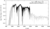 |
Fig. C.1. Flux-calibrated, extinction-corrected NIR spectrum of 2MASS J15361110-3444473 (in black) with its BT-Settl model (Teff = 2500 K and log g = 4.5, in grey). |
Appendix D: Updates with Gaia DR3
As stated in Sect. 2, we used the Gaia DR2 catalog to select our targets. Very recently, Gaia DR3 (Gaia Collaboration 2021) became public and gave us the opportunity to check the catalog for any possible changes or updates on the kinematic or stellar properties of our objects analyzed in this work. We did not find any considerable difference between the kinematic properties reported in both catalogs. However, we report the highlights of our search using these two catalogs in the following paragraphs.
As found in this work, for TYC 7335-550-1 we obtained Teff = 4488 K, while in both Gaia DR2 and Gaia DR3 its reported temperature is 5000 K. The reported RV for TYC 7335-550-1 in Gaia DR2 is 1.20 ± 1.65 km s−1, which is better constrained than the RV we report here (2.6±2.0km s−1). With regard to the wide companion candidate of 2MASS J15361110-3444473, we recalculated their Δv using the Gaia DR3 kinematic properties of TYC 7335-550-1, and it resulted in Δv = 5.34±3.30 (km s−1), which is consistent with the previous Δv = 4.72±3.47 (km s−1). For both of these calculations, we use the RVs calculated by ROTFIT.
The star Sz 70 has a high RUWE in both catalogs (4.86), but we saw no signs of binarity in the spectrum of Sz 70. Using the kinematic properties of Sz 70 reported in Gaia DR3 and those of Sz 71 (which is also updated in Gaia DR3), we recalculated their maximum velocity difference, and it resulted in Δv = 8.36±3.24 (km s−1), which is consistent with the Δv = 6.07±3.24 (km s−1) calculated based on Gaia DR2.
The star 2MASS J15414827-3501458 has a high RUWE (4.198) in both Gaia DR2 and Gaia DR3 catalogs, but we detected no signs of binarity in the spectrum of the object. We report that the kinematic properties of all our targets (parallax and proper motions) are consistent within 3σ in the two catalogs. Also according to Manara et al. (2022), we do not expect the stellar physical parameters of our core sample to be changed with the astrometry reported in Gaia DR3.
All Tables
Lupus I core members known from the literature (measurement errors are displayed in parenthesis).
Objects observed with X-shooter (measurement errors are displayed in parentheses).
EWs of the relevant lines indicating the chromospheric and accretion tracers for our targets.
EWs of the relevant lines indicating the chromospheric and accretion tracers for TYC 7335-550-1.
Disk categorization of all our targets, in addition to their reddest colors available in the 2MASS and WISE catalogs.
Kinematic properties of the Lupus I members from this work (measurement errors are displayed in parentheses).
Core members of Lupus I sharing similar kinematic properties (measurement errors are displayed in parentheses).
Astrometric properties of the candidate Lupus I members that were not observed by X-shooter, with their errors in parentheses.
Ages of our targets estimated using various isochrones. The ages are all in millions of years.
All Figures
|
Fig. 1. CMD of all the potential members of Lupus I in our original sample of 43 objects (blue dots), with the MS stars (Pecaut & Mamajek 2013) (orange dots) and the Lupus I core members (red triangles) included in Table 1. |
| In the text | |
|
Fig. 2. J − H (mag) versus H − Ks (mag) diagram of all our targets. The red dots show the chromospherically dominant targets, the cyan dots are the accretors, and the blue line represents the colors of MS objects down to spectral type M9.5. The normal reddening vector, shown with the black arrow, corresponds to AV = 2 mag. The rightmost target is 2MASS J15361110-3444473 which is suspected to be a binary; hence, it might have color contribution from a second target. |
| In the text | |
|
Fig. 3. |EWHα| versus SpT of our targets with the weak lined T Tauri stars studied by Manara et al. (2013, blue dots). The cyan dots represent accretors, and the red dots represent chromospherically dominant objects. The horizontal lines in red represent the thresholds that separate non-accreting and accreting objects considering their SpTs (White & Basri 2003). |
| In the text | |
|
Fig. 4. X-shooter spectrum of TYC 7335-550-1 in Hα region, normalized to the local continuum (black solid line) along with the inactive photospheric template (red dotted line). The latter is produced by ROTFIT with the BT-Settl synthetic spectrum at the Teff and log g of this target that is degraded to the resolution of X-shooter, rotationally broadened, and wavelength-shifted according to the target RV. The difference target-template is displayed at the bottom of the box and emphasizes the Hα emission that fills in the line core (green hatched area), which has been integrated to obtain the Hα line flux. |
| In the text | |
|
Fig. 5. X-shooter spectra of TYC 7335-550-1 in various wavelength portions. (a) X-shooter UVB spectrum of TYC 7335-550-1 in the Ca II H&K region (black solid line) along with the inactive photospheric template (red dotted line). (b) and (c) Residual (target-template) spectrum around the Ca II K and Ca II H lines, respectively. The hatched green areas mark the residual H and K emissions that have been integrated to obtain the EWs and fluxes. The purple-filled area relates to Hϵ. (d) and (e) Observed Ca II IRT line profiles (black solid lines) with the photospheric template overlaid with red dotted lines. The residual spectra are shown at the bottom of each panel shifted downward by 0.2 in relative flux units for clarity. |
| In the text | |
|
Fig. 6. RV of our accretors (cyan dots), chromospherically dominant targets (red dots), and the Lupus I core members (black dots). |
| In the text | |
|
Fig. 7. log L⋆(L⊙) versus log Teff (K) diagram for all our targets (cyan and red dots represent accretors and non-accretors, respectively), together with the previously characterized Lupus members (black dots, Alcalá et al. 2019, subluminous objects are not plotted). Blue dashed lines represent evolutionary tracks of Baraffe et al. (2015) for stars with masses indicated by the number (in M⊙) next to the top or bottom of each track. The red lines indicate isochrones calculated with the same models at ages of 1, 3, 30 Myr and 10 Gyr, from the right to the left. |
| In the text | |
|
Fig. 8. Log ⟨Lacc/L*⟩ versus Teff for all our targets. The cyan dots represent accretors and the red dots represent chromospherically dominant targets. The lines indicate the limit below which the chromospheric activity for a star is dominant (Manara et al. 2017), for two regimes of stars with Teff ≤ 4000 K (the diagonal blue line) and those with Teff ≥ 4000 K (the horizontal orange line). |
| In the text | |
|
Fig. 9. Log Macc(M⊙/yr) versus log M*(M⊙) for the four accretors in our sample (cyan dots), together with the previously identified members of the Lupus (black dots). The blue crossed squares represent the sub-stellar accreting companions detected at wide orbits by Zhou et al. (2014) around GQ Tau, GSC 06214 00210, and DH Tau as labeled. 2MASS J15551027-3455045, GQ Lup c and 2MASS J16085953-3856275 are also labeled. 2MASS J15523574-3344288 is labeled as a red dot. The continuous red line indicates the double power-law prediction of Vorobyov & Basu (2009), while the magenta dashed line shows the prediction of the disk fragmentation model by Stamatellos & Herczeg (2015). |
| In the text | |
|
Fig. 10. BT-Settl models (in gray) with the photometric data (red dots) for our accretors. |
| In the text | |
|
Fig. 11. BT-Settl models (in gray) with the photometric data (red dots) for our chromospherically dominant targets. |
| In the text | |
|
Fig. 12. Log-log plot of total velocity difference Δv (km s−1) versus projected separation (au) for the wide companion candidates analyzed in this work, in addition to the genuine wide companions GQ Lup and GQ Lup C. Δvmax (km s−1) (orange line) indicates the maximum total velocity difference that bound binaries with a total mass equal to 10 M⊙ in circular orbits can possess (Andrews et al. 2017). Each point is marked as one of the wide companion candidates involved. For the detailed information (see Tables 12 and 13). |
| In the text | |
|
Fig. C.1. Flux-calibrated, extinction-corrected NIR spectrum of 2MASS J15361110-3444473 (in black) with its BT-Settl model (Teff = 2500 K and log g = 4.5, in grey). |
| In the text | |
Current usage metrics show cumulative count of Article Views (full-text article views including HTML views, PDF and ePub downloads, according to the available data) and Abstracts Views on Vision4Press platform.
Data correspond to usage on the plateform after 2015. The current usage metrics is available 48-96 hours after online publication and is updated daily on week days.
Initial download of the metrics may take a while.