© The Authors 2023

1. Introduction

The Crab Nebula and pulsar are the centrepieces of gamma-ray astronomy and high energy (HE) astrophysics in general. The discovery of its very high energy (VHE) emission by the pioneering observations with the Whipple air Cherenkov telescope (Weekes et al. 1989) marks a breakthrough in the field by establishing the Crab Nebula as the brightest steady gamma-ray source.

The current understanding of the nebula was already established several decades ago by Rees & Gunn (1974). The description of the dynamics of the nebula and its radiative model dominated by synchrotron emission of relativistic electrons (Pacini & Salvati 1973) has remained basically unchanged for the past 50 years. In this model, the nebula is powered by a continuous cold and ultra-relativistic pulsar wind. The wind terminates at a distance of about 0.13 pc (Weisskopf et al. 2012) to the pulsar in a standing shock. The position of the termination shock is commonly associated with the bright ring observed at soft X-rays which has a major axis of (13.3 ± 0.2)″ (Weisskopf et al. 2012)¹.

The slow expansion of the nebula requires the downstream flow to slow down. In an ideal magneto-hydrodynamic (MHD) setting as suggested by Kennel & Coroniti (1984), the ratio of magnetic to kinetic energy (σ parameter) upstream of the shock is estimated to σ = 0.003 to match the boundary conditions of the slow expansion of the outer nebula of ≈1500 km s⁻¹. In the downstream flow, the toroidal (‘wound up’) magnetic field would increase due to magnetic flux conservation with increasing distance until equipartition is reached.

However, with the three-dimensional treatment of the MHD problem (Porth et al. 2013) it has been demonstrated that the magnetic field structure and magnetic field present in the plasma very likely deviate from the simplified model of Kennel & Coroniti (1984). Additionally, the conversion of ordered fields to turbulent fields which would be dissipated in non-ideal MHD plasma could change the magnetic field configuration substantially (Bucciantini et al. 2017; Tanaka et al. 2018).

The spatially resolved degree of polarisation and position angle in the radio (e.g., Bietenholz & Kronberg 1990) and optical (e.g., Hickson & van den Bergh 1990) indicate the presence of large-scale toroidal fields in the region of the torus, while at larger distances the field orientation becomes predominantly radial as traced out in the radio. The fraction of polarised X-ray emission from the Crab Nebula was measured to be (19.2 ± 1)% (Weisskopf et al. 1978; Feng et al. 2020; Liu & Wang 2021), which indicates that the magnetic field energy is roughly equally shared between an ordered and small-scale turbulent field (Bucciantini et al. 2017). A more detailed view of the spatial distribution of the magnetic fields will be possible with the upcoming observations of the Crab Nebula with the Imaging X-ray Polarimetry Explorer (IXPE; Weisskopf et al. 2016).

With the observation of (inverse Compton) generated gamma-ray emission, the ideal MHD flow-type solution (Kennel & Coroniti 1984) has been confirmed to provide a reasonable description of the nebula’s gamma-ray spectrum (Atoyan & Aharonian 1996). Improved spectroscopy at VHEs demonstrates however, that the simple approach does not provide a reasonable description of the data anymore (Aleksić et al. 2015). Even though the ideal MHD flow solution and its siblings remain as benchmarks (see e.g., Abdalla et al. 2020), the observational data are of sufficient quality to test the underlying assumptions of the simple flow model already developed in the 1970s.

So far, it has not been possible to spatially resolve the magnetic field strength in the nebula or any other pulsar wind nebulae. High energy and VHE gamma-ray observations have been used to estimate an average magnetic field from the ratio of synchrotron to inverse Compton emission (Aharonian et al. 2004), which requires careful modelling of the seed photon fields in the nebula (Meyer et al. 2010). Even though this method is robust, observational details, which are required to match the precision of the observational data with sufficiently accurate model calculations, have been mostly omitted in past studies.

In this analysis, we take the next step and include the recent measurement of the spatial extension at gamma rays of the nebula (Yeung & Horns 2019; Abdalla et al. 2020) in combination with the most recent spatial and spectral multi-wavelength data to reconstruct, for the first time, the electron and magnetic field configuration in the nebula in a consistent phenomenological model without any underlying assumptions as to the flow properties.

The underlying parameters were estimated with a χ² minimisation method. This is the first study of this type carried out on any gamma-ray emitting source. Thanks to the exceptional multi-wavelength observational data, the Crab Nebula remains a corner stone object for the study of non-thermal processes in relativistic plasma.

2. Observations

In the following, the heliocentric distance of the Crab Nebula is assumed to be d_Crab = 2 kpc (Trimble 1973). The basis of the compilation of multi-wavelength data used here is summarised by Aharonian et al. (2004), Meyer et al. (2010) and references therein. In the past decade, both new observations (see Table 1) as well as refined and relevant corrections on the extinction in the interstellar medium have become available.

2.1. Radio and infrared observations

The transition between the radio synchrotron component and the thermal dust emission is explored through observations with the Herschel (PACS and SPIRE), Spitzer (MIPS), while the transition from the dust emission to the optical/wind synchrotron emission is traced with WISE and Spitzer (IRAC) multi-band photometry. The integrated aperture-photometry (integrating over an ellipse centred on the pulsar position, with PA = 40° and semi-major and minor axes of 245″ × 163″) is taken from De Looze et al. (2019), Table 3. In addition to the continuum component, the emission lines contribute up to 18% of the continuum flux in the PACS λ = 100 μm pass band. The resulting data set is shown in Fig. 1 in combination with the best-fitting model. The new and additional data taken from the compilation of De Looze et al. (2019) are marked with white circles in Fig. 1.

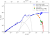Fig. 1. Observed spectral energy distribution (SED) from radio to optical photon energies. The additional data from the recent compilation of photometric data from De Looze et al. (2019) are marked with white circles. Optical/UV data are presented with and without extinction correction (see text for more details). The SED has been fit with the superposition of thermal dust emission (see Table 3 for a list of parameters and uncertainties) and the underlying synchrotron continuum (see Table 4).

2.2. Optical observations

In comparison to previous works (Meyer et al. 2010), the optical data used here have been updated to include a more recent estimate of the extinction along the line of sight towards the Crab Nebula. In the original compilation of Aharonian et al. (2006), the extinction was corrected using A(V) = 1.5 mag with a colour excess E(B − V) = 0.47 mag guided by the discussion of Véron-Cetty & Woltjer (1993). More recent 3D-reconstruction of the Galactic extinction with Gaia, Pan-STARRS 1, and 2MASS observations lead to a smaller value of A(V) = 1.2 mag (Green et al. 2019). We chose here the central value of A(V) = (1.08 ± 0.38) mag and E(B − V) = 0.43 mag determined by De Looze et al. (2019) from modelling the dust emission along the line of sight towards the Crab Nebula. The wavelength dependent extinction was calculated with the extinction curve from O’Donnell (1994). The resulting shape of the visual continuum emission follows a power law, such that I_ν ∝ ν^−s with s_O ≈ 0.8. This is considerably harder than the X-ray spectrum with s_X ≈ 1.3. The far-UV spectroscopy of the entire nebula with the Hopkins UV telescope (Blair et al. 1992) confirms the extrapolation of the optical spectrum to the UV. The UV spectrum obtained in a slit aperture of 17″ × 116″ displayed in Fig. 1 was corrected by an ad hoc correction factor of 7.5 to match the overlapping photometric points of Hennessy et al. (1992).

Additionally, we extracted the spectral indices s(9241 − 5364) obtained between λ = 9241 Å and λ = 5364 Å from Fig. 1 of Véron-Cetty & Woltjer (1993). The spectral indices were determined within bins of 10″ × 10″ covering the optical nebula. By averaging over annuli centred on the pulsar position, we calculated the mean and root mean square of s_O. The indices change from ≈0.6 in the centre to ≈1 at the periphery of the nebula (see Fig. 2). This is well-matched by the predicted behaviour of the synchrotron model as indicated by the superimposed blue line in the same figure.

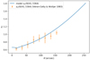Fig. 2. Predicted and observed optical spectra of the Crab Nebula. In concentric annuli, the mean and root mean square of the spectral indices sO (Iν ∝ ν−sO) have been determined from the data displayed in Fig. 1 of Véron-Cetty & Woltjer (1993). The superimposed curve is calculated from the intensity expected from the synchrotron model as described in Sect. 4.3 with the best-fitting parameters listed in Table 4. It is important to note that these data have not been used in the fit.

2.3. X-ray observations

The Crab Nebula has a long history as a standard candle for X-ray astronomy (Toor & Seward 1974). Therefore, for many X-ray telescopes the instrumental response functions are tuned to reproduce a particular spectral shape that is deemed to be a canonical X-ray spectrum following a power law dN/dE = N₀(E/keV)^−Γ, with Γ = 2.11 and N₀ = 11 in units of cm⁻² s⁻¹keV⁻¹, readers can refer to Shaposhnikov et al. (2012), for example.

In this spirit, the X-ray spectrum of the Crab Nebula has been used to cross-calibrate different instruments (Kirsch et al. 2005; Weisskopf et al. 2010). Given the apparent brightness of the nebula, other weaker non-thermal X-ray sources are conveniently used for more sensitive instruments which suffer from saturation/pile-up for bright sources such as the Crab Nebula. In a recent study of the non-thermal X-ray source G21.5-0.9 (Tsujimoto et al. 2011), the findings of earlier comparisons were confirmed that the energy spectra measured with different instruments in the energy range from 2 keV to 8 keV show relative differences in the normalisation of up to 20% and differences in the spectral index of ΔΓ = 0.1.

Different to most other X-ray instruments in use, the pn-camera of the XMM-Newton X-ray observatory has been calibrated without relying on the Crab Nebula as a standard candle (Strüder et al. 2001). The normalisation N₀ = 8.6 (Kirsch et al. 2005) found in observations of the nebula with the pn-camera in burst mode is consistently smaller than the normalisation found with other instruments.

The challenging task to (cross-)calibrate the past, current, and future X-ray missions is carried out by a consortium that formed shortly after the publication of Kirsch et al. (2005). The International Astronomical Consortium for High-Energy Calibration (IACHEC) recognises these systematic differences (Madsen et al. 2021) but there is still no consensus which measurement can be considered to be more reliable.

In the previous works (Aharonian et al. 2006; Meyer et al. 2010), we chose to re-scale measurements at higher energies to match the XMM-Newton result. In view of the recent measurements of the nebula’s X-ray spectrum with the NuSTAR telescope, we updated this approach. The absolute flux measurement reported by Madsen et al. (2017) uses stray light from the Crab Nebula in the focal plane of the NuSTAR telescope. Since the X-rays do not pass from the optical mirror assembly, the resulting flux determination does not suffer from the uncertainty of the energy dependent efficiency of the mirror assembly. Subsequently, the instrumental team of NuSTAR has changed their canonical Crab spectrum to Γ = 2.103 ± 0.001 and N₀ = 9.69 ± 0.02. This normalisation is 14% larger than the previously obtained value for the pn camera (Kirsch et al. 2005). Moreover, the NuSTAR measurement extends to hard X-rays and is consistent with, for example, the results from the coded mask imaging detector and spectrometer SPI on the INTEGRAL observatory (Jourdain & Roques 2009) as well as Earth occultation data taken with the BATSE instrument (Ling & Wheaton 2003). Both measurements indicate a break of the spectrum at an energy of approximately 100 keV.

Beyond the hard X-ray band, gamma-ray measurements rely on Compton scattering instead of photo-ionisation. The Comptel telescope on-board the Compton-Gamma-Ray-Observatory (CGRO) observed the Crab Nebula for 9 years (Kuiper et al. 2001). The resulting time-averaged energy spectrum between 0.75 MeV and 30 MeV follows a power law with photon index Γ = 2.227 ± 0.013 (Kuiper et al. 2001). While the power-law index is consistent with the one determined with INTEGRAL-SPI and BATSE data at lower energies, the flux normalisation of the Comptel measurement is systematically lower than the one obtained with BATSE and SPI data. From Fig. 31 of Kuiper et al. (2001), we estimated possible relative systematic deviations on the collection area from two different calibration methods to be 20%. In the data sample used to characterise the synchrotron component of the nebula for the fit, we introduced an ad hoc scaling of the Comptel flux by 1.3.

Even though this scaling is larger than the systematic uncertainty of the Comptel flux, it is well within the range of the combined systematic uncertainty when cross-calibrating between the very different types of detector. Clearly, the MeV energy range is most challenging and even though heroic efforts are under way to re-analyse the complete Comptel data set (Strong & Collmar 2019), a new mission is required to improve the situation in this poorly explored energy range (see e.g., the COSI mission Tomsick & COSI Collaboration 2022).

An additional concern in constructing the X-ray SED of the Crab Nebula is the variability of its X-ray (Greiveldinger & Aschenbach 1999; Ling & Wheaton 2003; Wilson-Hodge et al. 2011) and gamma-ray flux (Tavani et al. 2011; Abdo et al. 2011). The X-ray variability has been observed to occur mainly between 2001 and 2010 with an apparent relative amplitude of 2(4)% in the energy band < 15(15–50) keV on timescales of ≈3 years. In the preceding years of monitoring the Crab Nebula with the RXTE mission, the flux appears to remain constant (Wilson-Hodge 2012). The X-ray spectrum softened between 2009 and 2011 with a photon index changing from 2.14 to 2.17 as measured with RXTE-PCA (Wilson-Hodge 2012). We show in Fig. A.1 the combined hard X-ray light-curve between 2000 and beginning of 2022.

When comparing the recent average flux with the historical measurements of about 50 years ago (Toor & Seward 1974), possible long-term flux variations do not exceed the variations observed during the 20 years covered by Wilson-Hodge (2012). The origin of the variability is not clear but a systematic effect can be firmly rejected as the sole reason given that the variability has consistently been observed with independent instruments.

On a shorter timescale and at larger energies, the Crab Nebula shows rapid variations of the flux between 100 MeV and approximately 1 GeV. The flux can both increase by a factor of ≈8 over timescales of days (Buehler et al. 2012) and it can also drop below the average flux within a similar timescale (Yeung & Horns 2020).

For the characterisation of the time-average synchrotron spectral energy distribution we assume that the X-ray variability is averaged out during the long exposure. It is to be expected that the variability measured at soft to hard X-rays should translate in a similar variability in the VHE gamma-ray flux at TeV energies. So far, multi-year observations of the nebula with ground-based gamma-ray instruments such as HEGRA have only constrained the relative variability to be smaller than 10% (Aharonian et al. 2006).

The more volatile situation at the end point of the synchrotron spectrum is unlikely to change the inverse Compton emission of the nebula. This has been confirmed by simultaneous observations of flares with Fermi-LAT and ground-based gamma-ray telescopes: during these observations no correlated flux changes have been found (H. E. S. S. Collaboration 2014; Aliu et al. 2014). There may be however a measurable change of the PeV gamma-ray flux during high flux or flaring states (see Sect. 4.4.4).

In Fig. 3, the data points used for the fit are shown as blue markers together with measurements listed above. The blue line indicates the best-fitting synchrotron model which includes the Fermi-LAT data points between 70 MeV and 500 MeV (see below).

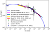Fig. 3. SED of the Crab Nebula centred on the X-ray energy range. The best-fitting model (blue line, see details on the fitting procedure in Sect. 4 and Table 4) is shown along with measurements from different X-ray observatories. The normalisation of the spectrum measured with XMM-Newton (yellow band) has been scaled up by 16% to be consistent with the absolute flux measurement with NuSTAR (magenta band). The COMPTEL gamma-ray flux has been scaled up by 30% to match the extrapolation of the SPI spectrum.

With the scaling of the flux measurements to match the absolute flux measurement of NuSTAR applied to the XMM-Newton and COMPTEL measurement, we obtain a consistent spectral measurement from 0.2 keV to 30 MeV. The spectrum in this energy range can be well characterised with a Band-like model (Band et al. 1993)

$$\begin{array}{c}\hfill \frac{\mathrm{d}N}{\mathrm{d}E}=N_0\{\begin{array}{cc}{\left(\frac{E}{100\mathrm{keV}}\right)}^{{\mathrm{\Gamma }}_1}{e}^{-E/E_0}\hfill & \text{if}E⩽E_0({\mathrm{\Gamma }}_1-{\mathrm{\Gamma }}_2),\hfill \\ {\left[\frac{({\mathrm{\Gamma }}_1-{\mathrm{\Gamma }}_2)E_0}{100\mathrm{keV}}\right]}^{{\mathrm{\Gamma }}_1-{\mathrm{\Gamma }}_2}{e}^{{\mathrm{\Gamma }}_2-{\mathrm{\Gamma }}_1}{\left(\frac{E}{100\mathrm{keV}}\right)}^{{\mathrm{\Gamma }}_2}\hfill & E>E_0({\mathrm{\Gamma }}_1-{\mathrm{\Gamma }}_2).\hfill \end{array}\end{array}$$(1)

with parameters for the photon indices Γ₁ = −2.095(4), Γ₂ = −2.34(1), E₀ = 1.36(17) MeV and normalisation at 100 keV: N₀ = 6.40(8)×10⁻⁴ cm⁻² s⁻¹ keV⁻¹. The resulting χ²(d.o.f.) = 97(158) indicates a good fit of the Band function. Similar parameters (Γ₁ = −1.99(1), Γ₂ = −2.31(2), E₀ = 531(30), N₀ = 7.5(2)×10⁻⁴ cm⁻² s⁻¹ keV⁻¹) have been obtained from analysing 17 years of INTEGRAL SPI data (Jourdain & Roques 2020), see also Fig. 3.

2.4. HE and VHE gamma-ray observations

Since the work of Meyer et al. (2010), roughly nine more years of Fermi-LAT observations have been presented in recent publications. Therefore, the statistical uncertainty on the flux above 100 GeV has been reduced by a factor of three. The updated instrumental response function of Fermi-LAT extends the HE reach from formerly 300 GeV to 500 GeV. The systematic uncertainty on the energy scale has been reduced from previously $\mathrm{\Delta }E/E{=}_{-10\%}^{+5\%}$ (see e.g., Abdo et al. 2009) to $\mathrm{\Delta }E/E{=}_{-5\%}^{+2\%}$ (Ackermann et al. 2012).

In a recent investigation of the gamma-ray extension of the Crab Nebula, Yeung & Horns (2019) analysed the LAT data accumulated over ≈9.1 years with a refined model for the Crab pulsar’s spectrum. They obtain a > 5 GeV spectrum of FL8Y J0534.5+2201i (the PWN component) which essentially matches the off-pulse spectrum reported by Buehler et al. (2012) but with improved statistical uncertainties and wider energy reach.

The MAGIC collaboration has published an updated energy spectrum of the Crab nebula overlapping the energy range covered with Fermi-LAT and reduced uncertainties at energies below 100 GeV (Aleksić et al. 2015). The measurement of the flux from the Crab Nebula with the MAGIC instruments spans for the first time from 50 GeV to 30 TeV. In a subsequent analysis of data taken with the MAGIC telescope at ultra-large zenith angles, the energy reach has been extended up to 100 TeV (MAGIC Collaboration 2020).

The VHE end of the Nebula’s spectrum has recently become a focus of interest with observational data taken with non-imaging air shower detectors with improved analysis of data taken with the HAWC water Cherenkov detector (Abeysekara et al. 2019) or with long-term observations with the Tibet ASγ air shower array which extends the energy spectrum up to 450 TeV (Amenomori et al. 2019). The latest addition to results on the Crab nebula obtained with the LHAASO KM2A array extends the spectrum beyond 1 PeV (LHAASO Collaboration 2021).

The High Energy Stereoscopic System (H.E.S.S.) collaboration has presented their preliminary results of H.E.S.S. phase II observations of the Crab Nebula Holler et al. (2015) superseding the results obtained with the previous setup (phase I) which consisted of four imaging Cherenkov telescopes (IACTs) with a mirror surface area of about 100 m² each and an energy threshold of approximately 100 GeV. Due to the visibility of the Crab Nebula from the southern hemisphere, the energy spectrum obtained with the phase I instruments from the Crab Nebula covers the energy range from 440 GeV up to 40 TeV (Aharonian et al. 2006). The large telescope of the H.E.S.S. phase II with a mirror surface of 600 m² has lead to a lowered energy threshold of 230 GeV for observations of the Crab Nebula (Holler et al. 2015).

Finally, the VERITAS collaboration has reported on observations of the Crab Nebula (55 h before and 46 h after the camera update in 2012; Wells 2019). In a previous analysis, slightly more data were used (Meagher & VERITAS Collaboration 2016), but the investigation of Wells (2019) indicate that the calibration of the two different levels of amplification for each channel need to be adapted. More detailed information on the VHE data sets is provided in Appendix A.

3. Non-thermal emission model

The specific luminosity L_ν from the Crab Nebula was calculated by integrating the synchrotron and IC emissivities ($j_{\nu }^{\text{Sy}}$, $j_{\nu }^{\text{IC}}$) over the volume of the nebula (assuming optically thin plasma and spherical symmetry):

$$\begin{array}{c}\hfill L_{\nu }=4\pi {\displaystyle {\int }_V{\mathrm{d}}^{3}r(j_{\nu }^{\mathrm{Sy}}(r)+j_{\nu }^{\mathrm{IC}}(r)),}\end{array}$$(2)

where the specific emissivity for inverse Compton emission ($j_{\nu }^{\text{IC}}$) and synchrotron emission ($j_{\nu }^{\text{Sy}}$) is given by

$$\begin{array}{c}\hfill j_{\nu }^{\mathrm{IC}}(r)=\frac{1}{4\pi }{\displaystyle \underset{\gamma }{\overset{\mathrm{d}}{\int }}\gamma n_{\mathrm{el}}(r,\gamma )\frac{3}{4}\frac{{\sigma }_{T}c}{{\gamma }^2}{h}^2\nu \underset{h\nu /4{\gamma }^2}{\overset{h\nu }{\int }}\frac{\mathrm{d}\epsilon }{\epsilon }{f}_{\mathrm{IC}}(\epsilon ,\nu ,\gamma )n_{\mathrm{seed}}(r,\epsilon ),}\end{array}$$(3)

$$\begin{array}{c}\hfill j_{\nu }^{\mathrm{Sy}}(r)=\frac{1}{4\pi }{\displaystyle \underset{\gamma }{\int }\mathrm{d}\gamma n_{\mathrm{el}}(r,\gamma )\frac{\sqrt{3}{e}^{3}B(r)}{m{c}^2}G\left(\frac{\nu }{{\nu }_c}\right),}\end{array}$$(4)

with n_seed(r, ε) and n_el(r, γ) being the differential number densities of seed photons and electrons respectively.

The resulting specific intensity I_ν(θ) was calculated by integrating along a line of sight subtending an angle θ with the centre of the nebula. The source region is optically thin. The external absorption in the interstellar medium was used to correct the apparent flux measurements in the optical/UV (de-reddening, see Sect. 2.2), X-ray (photo-ionisation, see Sect. 2.3), as well as at ultra-high energy (> 100 TeV) gamma-rays. The latter effect was re-evaluated here taking into account the anisotropy of the local radiation field which leads to an increase of the optical depth in comparison to previous works (see Appendix B for more details).

The function G(x) used for the synchrotron emissivity for an isotropic electron distribution in random magnetic fields (Crusius & Schlickeiser 1986) has been recently expressed in terms of modified Bessel functions as given in Eq. (D5) in Aharonian et al. (2010). For the numerical calculations, we used the convenient approximation of Eq. (D7) in Aharonian et al. (2010).

The function f_IC is the general function for scattering of electrons in an isotropic photon gas derived by Jones (1968; Eq. (44)).

In order to calculate the emissivity of the electrons we need to determine the electron distribution, seed fields, and magnetic field structure to reproduce all available observations. While the observed synchrotron emission is mostly degenerate for the choice of magnetic field and particle distribution, the observed inverse Compton emission breaks the degeneracy to allow us to reconstruct both the strength and the spatial variation of the magnetic field in the nebula.

3.1. Distribution of electrons

The spectral and spatial distribution of electrons in the nebula is inferred by matching a phenomenological model of the electron distribution and its synchrotron emission to observations. The electron distribution was kept as simple as possible and as complex as necessary to match the observations.

We assumed two different populations of electrons, so-called radio and wind electrons which do not share a common origin. While the wind electrons are most likely accelerated at the wind termination shock, the origin of the radio emitting electrons is not well understood. This includes both the generation of sufficient number of electrons/positrons as well as their acceleration. Recent suggestions include stochastic acceleration (Tanaka & Asano 2017), for example, in reconnection layers in the turbulent nebula (Lyutikov et al. 2019).

3.1.1. Spatial distribution of electrons

For photon energies below about 70 keV, the synchrotron emission is well-resolved by the available instruments. The observed (projected) structures are characterised by small-scale features (e.g., wisps) which evolve dynamically on timescales of weeks as well as large scale features including the X-ray bright ring, torus, and jets which remain stable for longer time-periods of years.

For the purpose of modelling the energy spectrum and extension of the inverse Compton emission of the nebula, we followed an approach similar to de Jager & Harding (1992), Hillas et al. (1998), Meyer et al. (2010) where the electron distribution is found by matching the expected synchrotron emission to the observed broadband spectral energy distribution (SED). In a second step, the magnetic field was determined by adjusting the electron distribution (mainly the normalisation) to match the observed inverse Compton emission to the data. In order to keep the model simple, the source was assumed to be spherical. Given the coarse angular resolution of the instruments used to observe the nebula at the HE end, this simplification is acceptable.

An important benefit of the assumption on spherical symmetry is the simple characterisation of the extension of the nebula. Here, we used the apparent angular extension θ₆₈ which is defined by the angular radius which encompasses 68% of the total flux. For a helio-centric distance d_Crab of the Crab Nebula, the spatial radius R₆₈ relates to the apparent size R₆₈ ≈ θ₆₈ d_Crab. We assumed a distance d_Crab = 2 kpc.

We collected available observations in order to determine θ₆₈ for different photon energies. The resulting values of θ₆₈ are summarised in Table 2. The Chandra data points² indicate the 68% containment angular radius θ₆₈ of the Crab Nebula for different energy bands. For each energy band (0.5–1.2; 1.2–2; 2–7; 7–10 keV), the centroid of the background subtracted image was calculated. The value of θ₆₈ for each energy band was determined using the method of encircled count fraction (ecf_calc task of the CIAO package v4.13). The uncertainty on θ₆₈ is dominated by systematic uncertainties which were estimated by checking against effects of vignetting and background contamination. The NuSTAR X-ray telescope has been used to image the X-ray nebula for the first time in a broad energy range from 3 keV–78 keV (Madsen et al. 2015). We estimated θ₆₈ from their Fig. 13 in three energy ranges. In the lowest energy band (3 keV–5 keV), the extension derived from the NuSTAR observations is about 5% smaller than the values obtained with the Chandra image, well within the estimated uncertainties of the two measurements.

The differential electron number density dn = n_el(γ, r)dγdV was assumed to follow a multiple broken power law in Lorentz factor γ (see below) with a spatial distribution approximated by a radial Gaussian with a the scale length ρ(γ) that depends on the electrons’ energy:

$$\begin{array}{c}\hfill n_{\mathrm{el}}(\gamma ,r)=n(\gamma )e^{-\frac{r^2}{2\rho {(\gamma )}^2}},\end{array}$$(5)

such that the predicted synchrotron emission matches the observed synchrotron extension.

The observed synchrotron size is mostly decreasing with increasing frequency, reflecting the cooling of the electrons as they propagate outwards. Therefore, we assumed for the wind-electrons a power law for ρ(γ):

$$\begin{array}{c}\hfill \rho (\gamma )=\frac{{\rho }_0}{{3600}^{″}}·\frac{\pi }{{180}^{°}}·\frac{d_{\mathrm{Crab}}}{2\mathrm{kpc}}{\left(\frac{B_0}{264\mathrm{\mu }\mathrm{G}}{\left(\frac{\gamma }{9\times {10}^5}\right)}^2\right)}^{-\beta },\end{array}$$(6)

with ρ₀ (in arc sec), B₀, and β > 0 free parameters in the fit to the data (see below).

Different to the wind electrons, for the low energy, radio-emitting electrons, the radial scale length ρ_r is independent of the electrons’ Lorentz factor. The value of ρ_r was left to vary freely in the fit to match the measured synchrotron extension.

3.1.2. Spectral distribution of electrons

We considered two distinctly different populations dubbed radio electrons as they are mostly emitting in the radio band and so-called wind electrons which are producing the bulk of the emission from optical to gamma-rays via synchrotron processes:

$$\begin{array}{c}\hfill n_{\mathrm{el}}(r,\gamma )=n_{\mathrm{radio}}(r,\gamma )+n_{\mathrm{wind}}(r,\gamma ).\end{array}$$(7)

The differential number density of each population was assumed to follow as a power law for the radio electrons

$$\begin{array}{c}\hfill n_{\mathrm{radio}}(r,\gamma )=N_{r,0}{\rho }_r^{-3}{e}^{-\frac{r^2}{2{\rho }_r^2}}{\gamma }^{-s_r}H(\gamma ;{\gamma }_0,{\gamma }_1),\end{array}$$(8)

and a broken power law for the wind electrons

$$\begin{array}{cc}& n_{\mathrm{wind}}(r,\gamma )=N_{w,0}\rho {(\gamma )}^{-3}{e}^{-\frac{r^2}{2\rho {(\gamma )}^2}}[{\left(\frac{\gamma }{{\gamma }_{w1}}\right)}^{-s_1}{\left(\frac{{\gamma }_{w1}}{{\gamma }_{w2}}\right)}^{-s_2}H(\gamma ;{\gamma }_{w0},{\gamma }_{w1})\hfill \\ \hfill & +{\left(\frac{\gamma }{{\gamma }_{w2}}\right)}^{-s_2}H(\gamma ;{\gamma }_{w1},{\gamma }_{w2})+{\left(\frac{\gamma }{{\gamma }_{w_2}}\right)}^{-s_3}H(\gamma ;{\gamma }_{w2},{\gamma }_{w3})]\hfill \end{array}$$(9)

respectively. The auxiliary function H(γ; γ₀, γ₁):=Θ(γ₁ − γ)Θ(γ − γ₀) with the Heaviside function Θ(x) defines the intervals of the broken power law.

A representative electron number density n_el at various distances and volume averaged is shown in Fig. 4. Note, the distribution of electrons follows a phenomenological Ansatz guided by the notion that electrons lose energy (radiative and adiabatic losses) while expanding in the nebula. However, without further knowledge about the properties and dynamics of the flow and the various and competing processes at work, the structure of the nebula can only be generically explained through the idea of a shock-accelerated electron distribution in a (ideal) MHD flow of a relativistic plasma as suggested for example by Rees & Gunn (1974) and following works (e.g., Kennel & Coroniti 1984).

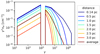Fig. 4. Electron number density nel, as a function of γ for different values of the distance to the centre of the Crab Nebula r and the volume average. The parameters used here are listed in Table 4.

In the absence of a specific model that matches available observations, we followed the approach of reconstructing the energy distribution of electrons and their spatial distribution from the observations. In this approach, we do not attempt to follow the temporal evolution of the nebula through its complex and largely unknown history.

3.2. Seed photon fields

The seed photon fields in the nebula were self-consistently calculated and matched to the observed intensity and brightness of the nebula. Note, in many previous attempts to model the nebula, the seed photon fields are assumed to be mostly homogeneous in the nebula and not specifically modelled to match the observations.

Assuming an isotropic specific volume emissivity j_ν (in 4π solid angle) in a spherical source, the spectral number density dn = n_seed(r, ε)dVdε of seed photons at a distance r to the centre of the nebula is:

$$\begin{array}{c}\hfill n_{\mathrm{seed}}(r,\epsilon )=\frac{4\pi }{h\epsilon }\frac{1}{2c}{\displaystyle {\int }_{r_{min}}^{r_{max}}\frac{r_1}{r}{j}_{\nu }(r_1,\epsilon )ln\left(\frac{r+r_1}{|r-r_1|}\right)\mathrm{d}{r}_1.}\end{array}$$(10)

The three main seed photon fields contributing to the IC scattering of the relativistic electrons in the Crab Nebula are: (i) the synchrotron radiation; (ii) the FIR ‘excess’ radiation which is attributed to the dust emission; (iii) the 2.7K cosmic microwave background radiation (CMB).

3.3. Thermal emission from dusty plasma

Observations at sub-millimetre and far-infrared wavelengths show an excess flux in comparison to the extrapolated synchrotron continuum alone. The excess is commonly modelled with the thermal emission of spherical, radiatively heated dust grains in thermal equilibrium (Marsden et al. 1984; Temim et al. 2006; Gomez et al. 2012; Temim & Dwek 2013; De Looze et al. 2019). A carbon dominated composition of the dust has been favoured in past studies where the temperature of the dust is either self-consistently modelled in combination with a dust grain composition (e.g., Temim & Dwek 2013) or estimated by fitting a two-temperature population to the data (e.g., De Looze et al. 2019). The dust emitting region is concentrated in the vicinity of the optical filaments which are forming a shell with inner radius of r = 0.55 pc (Čadež et al. 2004).

The observed emission in the wavelength band from λ ≈ 6 μm to λ ≈ 1000 μm is the superposition of continuum synchrotron and thermal dust emission as well as line-emission from excited atoms in the plasma. In Fig 1, the observed continuum emission is shown. In all previous works, a quantitative analysis of the dust emission has relied upon an ad hoc assumption on the underlying continuum emission.

Following the argument of Owen & Barlow (2015), we assumed the dust to be predominantly composed of amorphous carbon grains. The emissivity of dust grains in thermal equilibrium with a mass density ρ_d in the emitting volume is given by

$$\begin{array}{c}\hfill j_{\nu }={\rho }_d{\kappa }_{\mathrm{abs}}{B}_{\nu }(T),\end{array}$$(11)

with B_ν(T) denoting the black body spectral radiant emission at temperature T and κ_abs the mass absorption coefficient specific to the dust grain (Temim & Dwek 2013). In order to calculate the amount of seed photons present in the nebula which is relevant for the inverse Compton emissivity, we chose to fit a minimum set of free parameters to achieve an acceptable fit to the data. The minimal model found here is a mixture of dust at two different temperatures and with different values of mass (M₁, T₁, M₂, T₂). An additional parameter is the outer radius r_out of the dust population. The value of r_out needs to be adjusted to match the observed extension which is the result of the superposition of the underlying synchrotron continuum emission and the thermal emission of the dust. With the emissivity

$$\begin{array}{c}\hfill j_{\nu }=\frac{3{\kappa }_{\mathrm{abs}}}{4\pi (r_{\mathrm{out}}^3-r_{\mathrm{in}}^3)}[M_1{B}_{\nu }(T_1)+M_2{B}_{\nu }(T_2)]H(r;r_{\mathrm{in}},r_{\mathrm{out}})\end{array}$$(12)

of the two temperature dust model for a a fixed set of grain parameters (see next paragraph and Table 3) we achieved an acceptable description of the data (see Fig. 1).

The mass absorption coefficient κ_abs depends upon the geometry of the dust grain and the optical constants for the bulk material. Here, we used the measured optical constants of the ACAR sample (Zubko et al. 1996) and calculated the resulting values of κ_abs assuming a spherical symmetry and following the Mie-scattering theory in a series expansion. The underlying calculation was carried out with the numerical algorithm described in Bohren & Huffman (1998), Appendix A. A more thorough self-consistent modelling of the dust emission by radiatively heated dust grains is left for further work. The grains’ diameter distribution was assumed to follow a power law between the minimum grain radius a_min = 10⁻³ μm and a_max = 0.1 μm such that the probability density of finding a grain between a and a + da is given by p(a)da = p₀a^−s with s = 4 for a in the interval [a_min, a_max] (Temim & Dwek 2013). In the relevant range of wavelengths (from λ = 1 μm to λ = 10³ μm), the resulting opacity is conveniently approximated with

$$\begin{array}{c}\hfill {\kappa }_{\mathrm{abs}}=2.15\times {10}^4\frac{{\mathrm{cm}}^2}{\mathrm{g}}{\left(\frac{\lambda }{\mathrm{\mu }\mathrm{m}}\right)}^{-1.3},\end{array}$$(13)

with relative deviations between the model (Temim & Dwek 2013) and the parametrisation of less than 5% between λ = 10 μm and λ = 200 μm.

The thermal line emission from the excited plasma was not considered here. In the visual band, the relative contribution of the line emission to the overall flux is approximately 30% when comparing the sum of the equivalent width of the lines listed in Table 2 of Smith (2003) with the wavelength-band of the measured spectrum.

3.4. Magnetic field structure

The widely used model for the confinement of the Crab Nebula by Kennel & Coroniti (1984) is based upon a toroidal magnetic field without any turbulence forming. Three-dimensional relativistic ideal MHD simulations supports the notion of disordering of the magnetic field (Porth et al. 2013) which has been argued to account for the slowing of the expansion velocity to match the observations (Tanaka et al. 2018) and the comparably small polarisation observed at X-rays (Bucciantini et al. 2017; Weisskopf et al. 1978). In non-ideal MHD plasma flows, dissipation of magnetic fields would need to be considered as well (Tanaka et al. 2018; Luo et al. 2020). In this type of extension of the pulsar wind nebula scenario, several of the fundamental short comings of the toroidal field model of the Crab Nebula (Kennel & Coroniti 1984) can be overcome as argued by Luo et al. (2020).

In the following, we assumed a model where the magnetic field is dominated by small-scale turbulence. The root mean square value B(r) follows a power law for its radial dependence:

$$\begin{array}{c}\hfill B(r)=B_0{\left(\frac{r}{r_{\mathrm{s}}}\right)}^{-\alpha },\end{array}$$(14)

with B₀ the field strength at the distance of the termination shock r_s = 0.13 pc and α ≥ 0 free parameters of the model. The value α = 0 corresponds to the case of a constant magnetic field as for example assumed by Meyer et al. (2010). The case α = −1 corresponds to an MHD flow dominated by kinetic energy (σ ≪ 1).

4. Parameter estimation

The complete model description of the non-thermal electron distribution (Eqs. (8) and (9)), the spatial distribution, temperature, and mass of the dust grains (Eq. (12)) as well as the strength and radial dependence of the magnetic field (Eq. (14)) requires one to choose values for the underlying parameters. The complete set of parameters were combined in a tuple Ψ = (Ψ₁, …, Ψ₂₁) (see Table 4 for the complete list of parameters and best fitting values found in Sect. 4.4.2).

The subset of parameters Ψ₁, …, Ψ₁₄ relates to the electron distribution and is closely related to the choice of the magnetic field with normalisation Ψ₂₀ = B₀ and power-law index Ψ₂₁ = α for the radial distribution (see Eq. (14)). The parameters Ψ₁₅, …, Ψ₁₉ characterise the dust distribution and the amount and temperature of the two dust populations (see Eq. (12)).

4.1. Data sets used

The method to estimate the best-fitting values Ψ is based upon the minimisation of the sum of χ² values calculated for the two compilations of observational data. 𝒟_sync and 𝒟_IC (see the following Sect. 4.2 on the definition of the test statistics).

The observational data set 𝒟_sync includes 203 flux measurements f_ν and uncertainties σ_f³ as well as 15 measurements of the angular extent (see Table 2) ${\theta }_{68}^{\text{obs}}(\nu )$) and corresponding uncertainties σ_θ(ν). The resulting synchrotron data set

$$\begin{array}{c}\hfill {\mathcal{D}}_{\mathrm{sync}}={\mathcal{D}}_{\mathrm{sync},\mathrm{SED}}\cup {\mathcal{D}}_{\mathrm{sync},\mathrm{ext}},\end{array}$$(15)

is the union of the spectral measurements

$$\begin{array}{c}\hfill {\mathcal{D}}_{\mathrm{sync},\mathrm{SED}}=\{(f_{\nu ,i},{\sigma }_{f,i})|i=1,\dots ,203\},\end{array}$$(16)

and the measurement of the angular (apparent) extension

$$\begin{array}{c}\hfill {\mathcal{D}}_{\mathrm{sync},\mathrm{ext}}=\{({\theta }_{68}({\nu }_j),{\sigma }_{\theta }({\nu }_j))|j=1,\dots ,15\}.\end{array}$$(17)

The spectral data set 𝒟_sync, SED comprises a variety of observations collected with different instruments. In many instances, the resulting measurements are mutually inconsistent indicating systematic uncertainties (see also Sect. 2 for more details). The quoted uncertainties on the flux measurements σ_f, i are limited to the statistical uncertainties.

While below energies of 1 GeV, the dominant contribution to the Crab Nebula’s luminosity is synchrotron emission of electrons and thermal emission from radiatively heated dust grains, at energies larger than 1 GeV, the dominant emission process is inverse Compton scattering of the same electron population on various seed photon fields present in the nebula.

For energies above 1 GeV, we compiled a data set 𝒟_IC

$$\begin{array}{c}\hfill {\mathcal{D}}_{\mathrm{IC}}={\mathcal{D}}_{\mathrm{IC},\mathrm{SED}}\cup {\mathcal{D}}_{\mathrm{IC},\mathrm{ext}},\end{array}$$(18)

which includes the measurements of the energy spectrum using Fermi-LAT data (25 data points: 𝒟_IC, SED) and the angular extension (𝒟_IC, ext: 8 measurements as listed in Table 2) combining Fermi-LAT (Yeung & Horns 2019) and H.E.S.S. measurements (H. E. S. S. Collaboration 2020). The spectral measurements obtained with H.E.S.S. and other ground-based instruments were included separately in the fitting procedure (see Sect. 4.4.2).

4.2. Cost functions

The approach followed here used combinations of cost functions χ²(𝒟_a, Ψ) calculated for the data sets 𝒟_a, where a indicates the underlying observations as given in Eqs. (15)–(18); for example, for the synchrotron SED:

$$\begin{array}{c}\hfill {\chi }_{\mathrm{sync},\mathrm{SED}}^2={\chi }^2({\mathcal{D}}_{\mathrm{sync},\mathrm{SED}},\mathrm{\Psi })={\displaystyle \sum _{i=1}^{203}\left(\frac{L_{\nu ,i}(\mathrm{\Psi })-4\pi d_{\mathrm{Crab}}^2{f}_{\nu ,i}}{4\pi d_{\mathrm{Crab}}^2({\sigma }_{f,i}^2+{(0.05f_{\nu ,i})}^2}\right),}\end{array}$$(19)

where L_ν, i is the model synchrotron luminosity at frequency ν_i. The statistical uncertainty on the flux measurement was adjusted by a systematic uncertainty, added in quadrature. Without further detailed knowledge about the contributions to the systematic uncertainty of individual measurements, we chose to assume that the flux measurements are subject to relative uncertainty of 5%⁴. The best-fitting parameters do not change within the accuracy of the minimising routine when varying the relative systematic uncertainty in the range from 0% to 7%.

The value of the model luminosity L_ν, i was calculated for a set of parameters Ψ (see Table 4). Furthermore, we calculated the χ²-statistics for the angular extension:

$$\begin{array}{c}\hfill {\chi }_{\mathrm{sync},\mathrm{ext}.}^2={\chi }^2({\mathcal{D}}_{\mathrm{sync},\mathrm{ext}},\mathrm{\Psi })={\displaystyle \sum _{j=1}^{15}{\left(\frac{{\theta }_{68}({\nu }_j,\mathrm{\Psi })-{\theta }_{68}({\nu }_j)}{{\sigma }_{\theta }({\nu }_j)}\right)}^2,}\end{array}$$(20)

where θ₆₈(ν_j, Ψ) was calculated from the intensity I_ν, j(θ), such that

$$\begin{array}{c}\hfill 0.68=\frac{{\int }_0^{{\theta }_{68}({\nu }_j)}\mathrm{d}\theta sin\theta I_{\nu ,j}(\theta )}{{\int }_0^{{\theta }_{\max }}\mathrm{d}\theta sin\theta I_{\nu ,j}(\theta )}.\end{array}$$(21)

The maximum value θ_max = 250″ was chosen such that the calculated angular extension θ₆₈ does not change within the numerical accuracy for a choice of a larger value of θ_max. The measured extensions and uncertainties are listed in Table 2. The uncertainties on the measured angular extension were estimated from the data and do not require additional adjustments as the resulting ${\chi }_{\text{sync},\text{ext}}^2$ (see Sect. 4.3) indicates an acceptable goodness of fit.

The value of

$$\begin{array}{c}\hfill {\chi }_{\mathrm{sync}}^2={\chi }_{\mathrm{sync},\mathrm{SED}}^2+{\chi }_{\mathrm{sync},\mathrm{ext}}^2\end{array}$$(22)

is the contribution to the cost function related to the synchrotron data set.

Similarly to the calculation of ${\chi }_{\text{sync}}^2$, the inverse Compton data set 𝒟_IC was used to calculate separately ${\chi }_{\text{IC},\text{SED}}^2$ and ${\chi }_{\text{IC},\text{ext}}^2$ and the sum of the two

$$\begin{array}{c}\hfill {\chi }_{\mathrm{IC}}^2={\chi }_{\mathrm{IC},\mathrm{SED}}^2+{\chi }_{\mathrm{IC},\mathrm{ext}}^2,\end{array}$$(23)

which is relevant to estimate the parameters related to the strength and radial distribution of magnetic fields in the nebula.

The main systematic uncertainty of the flux measurement with Fermi-LAT (see also Sect. 2) is related to the energy calibration of the calorimeter. This known uncertainty was taken into account by adding a contribution to ${\chi }_{\text{IC},\text{SED}}^2$ which relates to a relative scaling of the energy (frequency):

$$\begin{array}{c}\hfill \nu \mapsto {\nu }^{\prime }=\nu (1+\zeta ),\end{array}$$

such that

$$\begin{array}{cc}& {\chi }_{\mathrm{IC},\mathrm{SED}}^2={\displaystyle \sum _{i=1}^{25}\left({\frac{L_{\nu ,i}(\mathrm{\Psi })-4\pi d_{\mathrm{Crab}}^2{f}_{{\nu }^{\prime },i}}{4\pi d_{\mathrm{Crab}}^2{\sigma }_{f,i}}}^2\right)+}\hfill \\ \hfill & \mathrm{\Theta }(\zeta ){\left(\frac{\zeta }{0.02}\right)}^2+\mathrm{\Theta }(-\zeta ){\left(\frac{\zeta }{-0.05}\right)}^2.\hfill \end{array}$$(24)

The estimated systematic uncertainty allows for a relative shift in energy ζ to be a random deviate with a asymmetric normal distribution given by the quoted uncertainty on $\zeta =0_{-0.05}^{+0.02}$ (Ackermann et al. 2012). The value of ζ was found whenever evaluating ${\chi }_{\text{IC},\text{SED}}^2$ (see Sect. 4.4.1).

Finally, we included the contribution of the VHE spectral measurements to the cost function with ${\chi }_{\text{VHE}}^2$ (see Sect. 4.4.2).

In the following sections, we follow three different minimisation approaches, where the most general fit is presented in Sect. 4.4.2. Firstly, in Sect. 4.3, we minimise the cost function ${\chi }_{\text{sync}}^2$ (see Eq. (22)) on a grid of values for B₀ and α, demonstrating, that the synchrotron data set provides only a weak constraint on the parameter α and is degenerate for B₀. Secondly, we proceed in Sect. 4.4 with the inverse Compton component which allows us to lift the degeneracy with respect to B₀. In Sect. 4.4.1, the sum of ${\chi }_{\text{IC}}^2$ (Eq. (23)) and ${\chi }_{\text{sync}}^2$ is evaluated on the same grid of B₀ and α as in the previous approach. Finally, in the most general (time-consuming) fit in Sect. 4.4.2, the cost function ${\chi }_{\text{sync}}^2+{\chi }_{\text{IC}}^2$ is used for marginalising over 20 parameters (Ψ_1⋯20). The resulting model is used to calculate ${\chi }_{\text{VHE}}^2$ and consequently ${\chi }_{\text{tot}}^2(\alpha )={\chi }_{\text{sync}}^2+{\chi }_{\text{IC}}^2+{\chi }_{\text{VHE}}^2$ is used to find the best estimate for α.

4.3. Fitting the synchrotron spectrum and extension

Since we are mainly interested in the best-fitting values of Ψ₂₀ = B₀ and Ψ₂₁ = α, we marginalised over Ψ_1⋯19 such that we used the parameters ${\check{\mathrm{\Psi }}}_{1\cdots 19}$ which minimise ${\chi }_{\text{sync}}^2$ for a given pair of α, B₀. The resulting

$$\begin{array}{c}\hfill {\chi }_{\mathrm{sync}}^2(\alpha ,B_0)={\chi }^2({\mathcal{D}}_{\mathrm{sync}},\alpha ,B_0,{\check{\mathrm{\Psi }}}_{1\cdots 19}),\end{array}$$(25)

depends on α and B₀ only.

As a demonstration of the approach, we show in Fig. 5a the increment $\mathrm{\Delta }{\chi }_{\text{sync}}^2(\alpha ,B_0)$ relative to the value of the global minimum ${\chi }_{\mathrm{sync}}^2(\check{\alpha },{\check{B}}_0)$

$$\begin{array}{c}\hfill \mathrm{\Delta }{\chi }^2(\alpha ,B_0)={\chi }_{\mathrm{sync}}^2(\alpha ,B_0)-{\chi }_{\mathrm{sync}}^2(\check{\alpha },{\check{B}}_0).\end{array}$$(26)

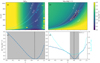Fig. 5. Results of the fitting procedure. Left column: (a) $\mathrm{\Delta }{\chi }_{\text{sync}}^2(\alpha ,B_0)$ and (c) $\mathrm{\Delta }{\chi }_{\text{sync}}^2(\alpha )$. Right column: (b) $\mathrm{\Delta }{\log }_{10}({\chi }_{\text{IC}}^2(\alpha ,B_0)+1)$ and (d) ${\log }_{10}(\mathrm{\Delta }{\chi }_{\text{IC}}^2(\alpha )+1)$. In the top panels, for each combination of α, B0, the other parameters of the model are marginalised; in the bottom panels, this includes B0. The dotted white lines in the top panels indicate the contours for constant values of volume averaged ⟨B⟩ = 30, 60, 90 μG. The cyan dashed line indicates the combinations B0 and α with the minimum total energy Wtot in electrons and magnetic field. The yellow solid contour marks the 95% confidence level error box for B0, α. The grey boxes in the bottom panel indicate the 95% confidence interval for α. In the bottom right diagram, the cyan dashed line indicates the minimal total energy Wtot for a given α. For a discussion on the relevance of the co-location of the global minimum ${\chi }_{\text{IC}}^2$ with the corresponding global minimum of Wtot, see the text.

For a constant value of α, the resulting ${\chi }_{\text{sync}}^2(\alpha ,B_0)$ does not change substantially over the range of B₀ ∈ [50 μG, 1025 μG] used in the scan with a step-size of ΔB₀ = 25 μG.

We find a global minimum for ${\chi }_{\text{sync}}^2$ at $\check{\alpha }=0.9$ with an uncertainty of σ_α(95%c.l.) ≈ 0.8 (see bottom left panel, Fig. 5c).

The parameter B₀ is the normalisation of the magnetic field at the position of the shock r_s. The resulting field ⟨B⟩ averaged over the volume from r_s to r_PWN = 3 pc was calculated to be

$$\begin{array}{c}\hfill ⟨B⟩=\frac{1}{V}{\displaystyle \int }\mathrm{d}VB(r)=\frac{3B_0{r}_{\mathrm{s}}^{\alpha }}{3-\alpha }\frac{r_{\mathrm{PWN}}^{3-\alpha }-r_{\mathrm{s}}^{3-\alpha }}{r_{\mathrm{PWN}}^3-r_{\mathrm{s}}^3}.\end{array}$$(27)

In Fig. 5a we plot contours for ⟨B⟩/μG ∈ {30,  60,  90} for orientation.

For a fixed value of α, ${\chi }_{\text{sync}}^2$ is degenerate for any choice of the normalisation B₀. However, the energy in magnetic field

$$\begin{array}{c}\hfill W_{\mathrm{B}}={\displaystyle \int }\mathrm{d}V\frac{B{(r)}^2}{8\pi }\end{array}$$(28)

increases for increasing B₀ while the normalisation of the electron spectrum decreases and correspondingly, the energy in particles W_e

$$\begin{array}{c}\hfill W_{\mathrm{e}}={\displaystyle \int }\mathrm{d}V{\displaystyle \int }\mathrm{d}\gamma m_{\mathrm{e}}{c}^2\gamma n_{\mathrm{el}}(r,\gamma )\end{array}$$(29)

decreases monotonically with increasing B₀.

The minimum energy configuration for the total energy

$$\begin{array}{c}\hfill W_{\mathrm{tot}}=W_{\mathrm{e}}+W_{\mathrm{B}}\end{array}$$(30)

is reached for B₀ = 514 μG, which is slightly lower than the equipartition (W_e = W_B) field B_eq = 558 μG.

The best-fit result which minimises ${\chi }_{\text{sync}}^2$ = 195.2(197 d.o.f.) is reached for $\check{\alpha }=0.9$ and large uncertainties which go well beyond the range of parameters scanned here.

The fitting of the model to the synchrotron data 𝒟_sync provides an overall satisfying goodness of fit. The parameters related to the electron distribution and dust properties can be estimated accurately.

We identified the combinations of B₀ and α which lead to a minimum energy configuration for each scanned value of α. The resulting contour B₀ = B_min is indicated as a cyan dashed line in Fig. 5.

Even though the configuration of the system is expected to be close to the minimum or equipartition value of B₀, without additional information the normalisation B₀ is degenerate with the number density of the electrons and α is only weakly constrained. The latter parameter is mostly degenerate with the radial distribution of the electron density (Ψ₁₃ = β).

Additional information such as the inverse Compton emission needs to be incorporated in the fit to break these degeneracies and determine the parameters B₀ and α.

4.4. Fitting the inverse Compton spectrum and extension

The inverse Compton emissivity of the electrons is proportional to the product of number density of electrons and the energy density of the seed photon field (in the Thomson limit of inverse Compton scattering).

The observation of inverse Compton emission and its spatial extension breaks the degeneracy of the model parameters. Different to a fit to the synchrotron component alone (see previous section), no additional constraints as for instance equipartition or minimum energy are required to determine α and B₀.

4.4.1. HE SED and extension

In order to make the fitting numerically tractable and to get an overview on the best-fitting parameters, we carried out a minimisation following these steps⁵:

1. Choose α ∈ [0, 1.2], starting at 0, incremental by 0.05

2. For each value of α, marginalise over B₀: ${\chi }^2(\alpha )={\chi }^2(\alpha ,\check{B_0})$

3. Repeat steps (1) and (2) and locate the global minimum ${\chi }^2(\check{\alpha })$.

The minimisation carried out in step (2) relates to ${\chi }^2={\chi }_{\text{sync}}^2+{\chi }_{\text{IC}}^2$ with ${\chi }_{\text{IC}}^2={\chi }_{\text{IC},\text{SED}}^2+{\chi }_{\text{IC},\text{ext}}^2$ given by

$$\begin{array}{c}\hfill {\chi }_{\mathrm{IC},\mathrm{SED}}^2={\chi }^2({\mathcal{D}}_{\mathrm{IC},\mathrm{SED}},\alpha ,B_0,{\check{\mathrm{\Psi }}}_{1\cdots 19},\check{\zeta }),\end{array}$$(31)

and

$$\begin{array}{c}\hfill {\chi }_{\mathrm{IC},\mathrm{ext}}^2={\chi }^2({\mathcal{D}}_{\mathrm{IC},\mathrm{ext}},\alpha ,B_0,{\check{\mathrm{\Psi }}}_{1\cdots 19}).\end{array}$$(32)

Note, the values of the parameter estimates related to the electron and dust population ${\check{\mathrm{\Psi }}}_{1\cdots 19}$ were found by minimising ${\chi }_{\text{sync}}^2$ separately for each choice of parameters α, B₀. This leads to an acceptable computation time for a parameter scan.

The resulting ${\chi }_{\text{IC}}^2$(α) shows a minimum for $\check{\alpha }=0.8$ shown in Fig. 5d (bottom right panel). While ${\chi }_{\text{sync}}^2$ remains essentially constant over the entire scan range, ${\chi }_{\text{IC}}^2$ rises quickly towards the lower and upper boundary of the scan range. In order to accommodate the dynamical range of Δ${\chi }_{\text{IC}}^2$, the right hand panels of Fig. 5 show log₁₀(Δ${\chi }_{\text{IC}}^2$ + 1).

The best estimates for $\check{\alpha }=0.8_{-0.13}^{+0.16}$ and ${\check{B}}_0=(497\pm 43)\mathrm{\mu }\mathrm{G}$ are close to the minimum energy condition (B_0, min = 514 μG, see also cyan lines in Figs. 5c,d and 6).

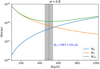Fig. 6. Volume-integrated total energy Wtot equals the sum of the energy in relativistic electrons We and magnetic field WB. For any best-fitting set of parameters, the energy partition is a function of the normalisation B0 of the magnetic field at the shock distance rs. The best-fitting value is found to be $\check{B_0}=(497\pm 43)\mathrm{\mu }\mathrm{G}$ (90% c.l. uncertainty, including systematical uncertainties). This value is slightly smaller than the minimal energy configuration at B0 = 514 μG.

For an overview of the best-fitting value ${\check{B}}_0$, we also carried out a scan in α, B₀ shown in Fig. 5b. The solid yellow contour in the same Figure indicates the 95% confidence level parameter region favoured here. The shape of the favoured parameter region follows the shape of the cyan line which traces the minimum energy configuration.

The fit to the synchrotron component is in comparison to the previous fit to the synchrotron component only slightly worse with ${\chi }_{\text{sync}}^2$ = 196.4 instead of ${\chi }_{\text{sync}}^2$ = 195.2 found in the previous section. The inverse Compton component is fit with ${\chi }_{\text{IC},\text{SED}}^2$ = 32.0 and ${\chi }_{\text{IC},\text{ext}}^2$ = 17.2. The total χ²(d.o.f.) = 245.6(228) indicates still an acceptable fit with p(χ² > 245.6, d.o.f. = 228) = 0.2. However, when considering the fit to the inverse Compton component only, the resulting ${\chi }_{\text{IC}}^2$(d.o.f.) = 49.2(29 indicates that the fit is not acceptable with p(χ² > 49.2, d.o.f. = 29) = 0.01.

Note, the best fit value for $\check{\alpha }$ is consistent for the two different estimates from fitting the synchrotron and inverse Compton data.

4.4.2. VHE SED

The fitting procedure outlined above has been primarily optimised for the synchrotron emission of the Crab Nebula (SED, extension). The inverse Compton component of the SED was mainly used to constrain independently from the electron spectral shape the magnetic field B₀ and the related parameter α.

Both, the synchrotron as well as the inverse Compton SED at energies below the peak in the SED are fairly degenerate for different choices of the radial dependence of the magnetic field (see also the following Sect. 4.4.3). The resulting uncertainty of the power-law index α used for B(r)∝r^−α is comparably large with σ_α ≈ 0.15, even after including the Fermi-LAT spectral information. Furthermore, when constraining the electron distribution by matching the synchrotron emission to the SED and determining in a separate step the best-fitting values of α and B₀ (see previous section), the resulting goodness of fit to the Fermi-LAT data is not acceptable.

The accurate measurement of the IC component at energies covered with ground based VHE gamma-ray telescopes bears the potential of determining α with greater precision. This is evident from the wide range of flux values and slopes of gamma-ray spectra at energies beyond several 100 GeV predicted for the interval of α considered here (see Sect. 4.4.3). Therefore, the VHE measurement of the SED reduces the uncertainty on the value of α.

We modified the method used in the previous section by including the LAT spectral information to estimate the parameters Ψ_1⋯20. This numerically expensive approach was necessary to improve the goodness-of-fit of the inverse Compton method and to include the VHE measurement.

The fit is carried out in the following steps:

1. Choose α ∈ [0.4, 0.8], increment by 0.005

2. Minimise ${\chi }^2(\alpha )={\chi }_{\text{sync}}^2+{\chi }_{\text{IC}}^2$ to estimate ${\check{\mathrm{\Psi }}}_{1\cdots 20}$

3. Calculate for each α the predicted VHE spectrum and the resulting ${\chi }_{\text{VHE}}^2$.

4. Repeat until the minimum ${\chi }^2(\check{\alpha })$ is found to estimate the parameter α.

The third step involves both individual VHE data sets 𝒟_VHE, i as well as their combinations.

$$\begin{array}{c}\hfill {\mathcal{D}}_{\mathrm{VHE}}=\bigcup _i{\mathcal{D}}_{\mathrm{VHE},i}.\end{array}$$(33)

A complete list of the data sets and individual fit results are presented in Appendix A and Table A.1. In the following, we considered a combination of five data sets obtained with MAGIC (normal zenith angles as well as very large zenith angles), VERITAS, Tibet ASγ, and LHAASO. With this combination of observations, a consistent model was found. Another consistent solution was found for the combination of the data from the HEGRA and HAWC observations (see Appendix C), while the spectra obtained with the H.E.S.S. I and II telescope arrays cannot be fit well by the model presented here (see Table A.1 for the individual fit results).

For each data set 𝒟_VHE, i, we introduced a relative energy scaling ζ_i as an additional nuisance parameter. This adjustment of the relative energy scale compensates for systematic uncertainties related to the absolute energy calibration of ground based air Cherenkov telescopes.

The scaling factors ζ_i determined for the VHE data are listed in Tab. 5. The values are close to unity with the largest correction applied to the MAGIC data set taken at very large zenith angles (MAGIC VLZA: ζ = 1.14 ± 0.03). The value found here is well within the error budget of the systematic uncertainty related to the energy scale which is estimated to be 17% for this data set (MAGIC Collaboration 2020). Note, the dramatic reduction of the χ² between ${\chi }_{\text{before}}^2=832$ before the scaling and ${\chi }_{\text{after}}^2=63.1$ after the scaling (see Tab. 5 for more details). The introduction of the five additional parameters reduces the number of degrees of freedom from 85 to 80 for the VHE data sets used here.

The best-fitting parameters were used to calculate the broadband SED for $\check{\alpha }=0.51\pm 0.03$ and ${\check{B}}_0=(264\pm 9)\mathrm{\mu }\mathrm{G}$ (for a complete list of parameters used, see Table 4). The result is shown in Fig. 7. The overall fit from radio to PeV energies traces the observational data with a resulting ${\chi }_{\text{SED}}^2={\chi }_{\text{sync},\text{SED}}^2+{\chi }_{\text{IC},\text{SED}}^2+{\chi }_{\text{VHE}}^2=182+24+41=247$ with 184 + 23 + 55 = 262 degrees of freedom (see Table 4 for the resulting parameter estimates as well as the goodness of fit summary). In the residual shown in the bottom panel of Fig. 7, deviations are visible in the MeV spectrum as well as at PeV energies. We return to possible explanations in Sect. 4.4.4.

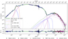Fig. 7. Best-fitting model in comparison to the data. The upper plot shows the synchrotron and inverse Compton (IC) radiation by radio (R) and wind (W) electrons produced in the spatially varying magnetic field and seed photon field (blue and magenta coloured broken lines indicate the contributions from IC scattering on individual seed photon fields). The blue data points are used in the fit to determine the parameters ${\check{\mathrm{\Psi }}}_{1\dots 20}$ listed in Table 4. The VHE data have been scaled using the values of ζi determined for each data-set (see text for further details) to adjust the energy scale for prediction given by the global minimum ${\chi }^2(\check{\alpha }=0.51)$. In the lower plot, the relative residuals are shown (statistical uncertainties only).

In more detail, the SED at HE and VHE gamma-rays is shown in Fig. 8. The VHE data sets selected are consistent after the relative energy scales have been slightly adjusted to a common energy-scale provided by the LAT data. The five different VHE data sets overlap in the energy range covered both with the LAT data as well as among each other. The resulting goodness of fit is quantified by ${\chi }_{\text{VHE}}^2$ = 41 for 55 degrees of freedom. Even without additional systematic uncertainties related to the flux measurement, the statistical uncertainties are not sufficiently small to further constrain or even rule out the model used here.

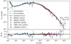Fig. 8. Comparison of the best-fitting model with the HE and VHE data. The detailed view confirms the consistency of the selected data sets (after scaling) and the good agreement of the model to the data. The selected VHE data sets overlap with the LAT data and each data set overlaps with at least one other VHE data set.

The spatial extension of the model emission is matching the measured extension quite well. This is shown in Fig. 9. The resulting ${\chi }_{\text{ext}}^2={\chi }_{\text{sync},\text{ext}}^2+{\chi }_{\text{IC},\text{ext}}^2=16+24=40$ for 15 + 8 = 23 data points (the number of degrees of freedom is reduced by the number of parameters of ≳2) indicates at first glance a poor fit: p(χ² > 40, d.o.f. = 21)≈1.2 × 10⁻⁵. However, the large value of ${\chi }_{\text{IC},\text{ext}}^2$ is mainly driven by one (outlying) measurement at E = 14 GeV. When removing that individual point, the resulting ${\chi }_{\text{ext}}^2(\text{d}.\text{o}.\text{f}.)=21(20)$.

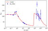Fig. 9. Extension of the model emission is characterised by the radial size θ68. The model curve is the calculated extension which matches well the observational data.

After including 𝒟_VHE, the constraint on the magnetic field distribution improved considerably. The best-fitting estimate for $\check{\alpha }=0.51\pm 0.03$ has a remarkably small statistical uncertainty. The value of α is mainly constrained by the accurate measurement of the SED at VHE energies. The measurement of the spatial extension is less constraining (see also Sect. 4.4.3). The difference in the best-fitting values for α when comparing the results obtained in Sect. 4.4.1 and the ones found here is not significant, but will be discussed in the context of an extension of the model in Sect. 5.5.

4.4.3. Varying α: Effect on the IC SED and extension

As discussed in the previous sections, there is a unavoidable degeneracy of ${\chi }_{\text{sync}}^2$ for variations of parameters related to the magnetic field (α, B₀) and the electron spectrum.

As an illustration of this degeneracy with respect to the choice of α, we show in Fig. 10 the best-fitting SEDs, colour-coded for different values of α. Each SED is the result of the fitting procedure outlined in Sect. 4.4.1 above. For clarity, the data points are not included.

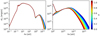Fig. 10. Overall spectral energy distribution for the estimated best-fitting parameters ${\check{\mathrm{\Psi }}}_{1\cdots 20}$ (after minimising ${\chi }_{\text{IC}}^2$ for fixed values of α) is shown. The value of α characterises the radial decrease of the magnetic field B ∝ r−α (see Eq. (14)). While the synchrotron part of the spectral energy distribution is almost degenerate with respect to the choice of α, the inverse Compton dominated part (right panel) shows noticeable differences up to the peak at approximately 1011 eV. Note, in the left panel the sum of synchrotron and inverse Compton emission is shown, while in the right panel, the SED of the inverse Compton emission is additionally superimposed.

The resulting SEDs indicate that the synchrotron component does not change in a noticeable way when varying the value of α while the inverse Compton emission varies in a systematic way: For a constant magnetic field (α = 0), the energy spectrum is harder than for models where the magnetic field drops with increasing radius (α > 0).

The model with the largest value of α = 1.2 covered in the scan has the softest spectrum. The differences between the models with varying α is most pronounced at the energies beyond the peak energy of approximately 100 GeV.

Similar to the SED, the angular extension of the synchrotron nebula is highly degenerate with respect to variations of the parameter α. This is demonstrated in Fig. 11.

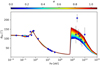Fig. 11. Angular extension from the fitting procedure described in the text. After marginalising ${\check{\mathrm{\Psi }}}_{1\cdots 20}$, the predicted angular extension of the synchrotron nebula matches the data well for values of α = 0, …, 1.1 with very small variations visible in the transition between thermal and non-thermal emission at near- to far infrared. At higher energies, the predicted size differs mostly at the low-energy end of the inverse Compton emission.

Different to the SED which shows the largest variations of the SED for the VHE part when changing the value of α, the angular extension varies the strongest for the part of the inverse Compton emission covered with HE gamma-ray observations.

At several GeV of gamma-ray energy, for a constant magnetic field, the extension is the lowest (about 100″) and it systematically increases with increasing α, such that for α = 1.2, the extension reaches a value of about 150″. At the highest energy part, the variation of the extension for different values of α is effectively constant.

The underlying reason for the observed changes in the SED is related to the magnetic field relevant for electrons of different energies. The most energetic electrons are located close to the shock which features the largest magnetic field. Consequently, a reduced number density of these electrons is required to match the synchrotron emission which in turn leads to a reduced inverse Compton emission, softening the VHE spectrum with increasing value of α. The energy range covered with Fermi-LAT is less affected by changes of α as the underlying electrons populate the entire volume and therefore produce synchrotron emission in an averaged magnetic field which does not change for the best-fitting model when varying α.

4.4.4. An additional ultra-high energy component

The energy spectrum measured at ultra-high energy (UHE) gamma-rays above several 100 TeV with the LHAASO array (LHAASO Collaboration 2021) apparently deviates from the predicted shape of the inverse Compton emission at the highest energy bin centred on E_γ = 1.26 PeV⁶. It has been speculated that the PeV emission could be due to an additional hadronic component, similar to the one possibly present in the Vela-X region (Horns et al. 2006). Previous upper limits on the presence of a hadronic wind have constrained the fraction of spin-down power diverted to the acceleration of relativistic hadrons to be less than ≈20% up to PeV energies (Aharonian et al. 2004). The PeV excess could be produced by as little as 1% of the spin down power assuming efficient confinement of the protons in the Crab Nebula (LHAASO Collaboration 2021).

Here, we invoked a second electron distribution similar to previous attempts of explaining the flaring component of the Crab Nebula (see e.g., Lobanov et al. 2011) with the energetic electrons located in the vicinity of the pulsar or close to the shock. The finding of a fast (several days) dimming in the Nebula’s emission (Yeung & Horns 2020) indicates that most of the highest energy synchrotron emission (> 75%) is produced in a compact region.

Motivated by these findings and the particular shape of the spectrum measured from the Crab Nebula with the COMPTEL instrument, we introduced a secondary PeV electron component which (on average) matches the highest energy part of the synchrotron spectrum. In the framework of the model developed here, we reduced the maximum energy of the wind electrons from γ_w3 = 4.8 × 10⁹ (E_w3 = 2.5 PeV) to γ_w3 = 2.5 × 10⁹ (E_w3 = 1.3 PeV). This way, the presumably steady synchrotron emission cuts off below 10 MeV (see Fig. 12).

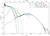Fig. 12. A suggested model for the SED including a secondary electron contribution located at the shock position. The low and high state spectra as measured with Fermi-LAT are shown for comparison (Yeung & Horns 2020). The secondary electrons’ spectrum during average (high) state is a power-law with dn/dγ ∝ γ−2.3 between γ1 = 3 × 109 and γ2 = 7(18)×109. The magnetic field in the region is chosen to be 85 μG. The total energy content of the electrons is 2(3)×1042 ergs. The dotted lines indicate the effect of absorption on the Galactic foreground emission (see also Appendix B).

We added a secondary component which is located at a fixed distance where due to radiative cooling, the energy is quickly dissipated. In the model considered here, the magnetic field varies as B(r) = 264 μG(r/r_s)^−0.51. In order to fit the synchrotron and UHE part, the consistent combination of seed photon field and magnetic field strength would favour a position in the nebula at r ≈ 20r_s. Since it seems unlikely that particle acceleration to PeV energies is ongoing in the nebula’s periphery, we explored here the possibility of electron acceleration close to the shock at r ≈ r_s, possibly in a region with weaker magnetic field strength (here, we chose a value of 85 μG). We considered the seed photon field at the shock self-consistently calculated in our model. We did not attempt a quantitative fit here but instead chose representative values in order to match the SED. The average additional electron spectrum was assumed to follow a power law with dn/dγ ∝ γ^−2.3 between γ₁ = 3 × 10⁹ and γ₂ = 7 × 10⁹.

The resulting spectra for the three flux states: wind-only with a reduced cut-off energy, average, and flaring PeV component are shown in Fig. 12 in comparison to the same data as shown before.

In addition, we include the low and high-state energy spectra provided by Yeung & Horns (2020) to compare with the respective flux state from the model. The total energy required in the secondary electron distribution is moderate with W_e = 2 × 10⁴² ergs.

The computed SED matches the data quite well. At the MeV energy range, the COMPTEL measurements are described better by the superposition of the steady wind electron emission and the average secondary component. During times of lower activity, the reduced cut-off in the wind electron spectrum matches the observed low-state spectrum Yeung & Horns (2020; dark green squares in Fig. 12).

The inverse Compton emission at energies beyond ≈400 TeV is dominated by the emission of the secondary component. The emission of the secondary component is produced by up-scattering of synchrotron (radio) seed photons and to a lesser extent by CMB photons.

We also included a model for the high flux state (light green curve in Fig. 12). The minimal modifications were an increase of maximum energy such that γ₂ = 1.8 × 10¹⁰ and an increase of the energy of the electrons to 3 × 10⁴² ergs. The resulting synchrotron emission matches the observation during the high flux state with Fermi-LAT quite well (light green circles). The resulting inverse Compton component during the high flux state is also shown in Fig. 12. In both cases, the absorption of gamma-rays due to the anisotropic Galactic radiation field is included (see Appendix B for details about the calculation carried out here).

5. Discussion of the parameters

5.1. Radio electrons

The four parameters Ψ_1…4 related to the radio electrons are well constrained by the observational data. The total number of radio emitting electrons has been found to be N_r ≈ 10⁵¹ up to a maximum Lorentz factor of γ₁ ≈ 90 000 for γ₀ = 22. The lower bound γ₀ = 22 has been fixed to a value which is not in conflict with the low frequency radio measurements starting at 111 MHz in our sample. A possible smaller value of γ₀ would increase the total number of radio emitting electrons. The value found here for N_r should be considered a lower limit.

The resulting total energy in radio electrons is 3.4 × 10⁴⁷ ergs (this value is determined by the value of γ₁). The spatial distribution of radio electrons is found to extend up to ρ_r = 89″ for the best-fitting model of the magnetic field B(r)∝r^−0.51. The resulting extension is therefore constant for the radio synchrotron emission which is in good agreement with the radial extension measured to be unchanged between 5 GHz and 150 GHz (see also Table 2).

The upper bound of the radio electron spectrum γ₁ is anti-correlated with the amount of cold dust (Ψ₁₇). The comparably low value for γ₁ found here is favoured by the observational data between λ = 100 μm and 1000 μm (see Fig. 1) where the dust emission starts to dominate over the synchrotron emission.

5.2. Dust emission

As a consequence of the comparably low value of the upper end of the radio electrons’ spectrum (γ₁), the amount of cold dust required here is larger than in previous estimates which were based upon a power-law extrapolation between the radio and optical. Using the same dust emissivities as De Looze et al. (2019), we therefore find for the cold dust mass a larger value (Ψ₁₇ = log₁₀(M/M_⊙) = − 1.2 ± 0.1) than previously (≈ − 1.7). In a standard (explosive) nucleosynthesis model (Woosley & Weaver 1995), the progenitor star would have to be sufficiently massive (M_prog ≥ 12(18) M_⊙) to produce the dust with 75(25)% condensation efficiency. The spatial distribution of the dust is confined to a shell with fixed inner radius 0.55 pc (see Sect. 3.3) and an outer radius estimated to be Ψ₁₅ = 1.53 ± 0.09 pc. This corresponds to an angle of ≈150″. This parameter is constrained by the angular size measured in the infra-red (see Table 2 and Fig. 9). The dust emissivity and resulting spatial distribution of dust generated seed photons (see Eq. (12)) was in turn used for the calculation of the IC emissivity (see Eq. (10)). The IC emission of wind electrons up-scattering the dust emission as seed photons dominates at the peak energy of a few 100 GeV. This is distinctly different from previous models where the dust seed photon field is assumed to maintain a constant energy density of 0.5…1 eV cm⁻³ throughout the nebula. Since the dust is formed in a shell surrounding the pulsar wind nebula, the energy density of the dust seed photon field reaches a maximum of ≈1.5 eV cm⁻³ at a distance of ≈1 pc (see Fig. 13).

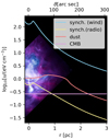Fig. 13. Energy density of the seed photons as a function of the distance from the pulsar. The dust emissivity was modelled to be confined in a shell surrounding the optical nebula. As a comparison, a composite of X-ray (Chandra: blue, white)/optical(HST: purple)/ infrared (Spitzer: pink) composite image from the nebula is shown with approximately matching spatial scale. Background image credit: X-ray: NASA/CXC/SAO; Optical: NASA/STScI; Infrared: NASA-JPL-Caltech).

5.3. Wind electrons

The spectral and spatial model of the wind electrons includes ten parameters (Ψ_5…14). Most of the electrons’ energy is carried by the wind electrons at the lower boundary γ_w0 = 320 000 (corresponding to E_w0 ≈ 200 GeV). The total wind electrons’ energy in the nebula is very close to the energy in radio electrons (3.4 × 10⁴⁷ ergs).

There is a considerable gap in energy between the two electron components (γ₁m_ec² ≈ 50 GeV vs. γ_w0m_ec² ≈ 200 GeV). The de-reddening of the optical nebula emission has revealed the presence of a further break in the spectrum between the optical and X-ray part (spectral index changes from 0.7 to 1.1). The break in the X-ray spectrum at about 120 keV requires a second break in the electron spectrum, such that we fitted as particle indices 3.1(2)→3.45(1)→3.77(4). The breaks are located at energies of γ_w1m_ec² ≈ 3 TeV and γ_w2m_ec² ≈ 110 TeV. The upper bound of the energy of wind electrons is fixed by the cut-off in the average synchrotron spectrum at γ_w3m_ec² ≈ 2.5 PeV. The power-law indices and the positions of the breaks are most likely intrinsic to the injected particle spectrum and the underlying acceleration mechanism. Similar results related on the position of the lower-energy break have been found by for example Martín et al. (2012). Radiative cooling would not be sufficient to explain however the appearance of the higher energy break at 110 TeV.

The spatial distribution of the wind electrons was assumed to be a radial Gaussian with an extension that follows a power law ρ(γ) = ρ₀γ^−β with index β = 0.15 (see Sect.3.1.1). The pre-factor ρ₀ for the wind electrons’ distribution was found to be (99 ± 4)″ which is larger than ρ_r = (89 ± 3)″ characteristic for the radio electrons. This fit result is a consequence of the comparably large size (≈145″) found at near infrared in the WISE images (see Table 2). The large value of ρ₀ is in line with the extension measured at high energies with Fermi-LAT (≈120″).

The observation that the lowest energy wind electrons with energies of approximately 200 GeV are distributed within a larger volume than the radio electrons indicates that the electrons are not only moving convectively with the wind.

5.4. PeV electrons

The most energetic electrons at PeV energies are traced by their synchrotron emission at energies of about 100 MeV observed with Fermi-LAT. The light curve of the 80…800 MeV synchrotron flux has been found to include at least three different spectral states (high, medium, and low state) that can be identified from Fermi-LAT observations (Yeung & Horns 2020): The high state is evident from the observation of flaring activity which occur roughly once per year (Mayer et al. 2013; Yeung & Horns 2020). In a flaring state, the flux increases during several days dramatically with a spectral hardening and a peak in the SED reaching up to several 100 MeV. The average high flux state spectrum as defined by Yeung & Horns (2020) is shown in Fig. 12. Despite large efforts (Weisskopf et al. 2013), no obvious counter-part to the flares has been identified, even though the optical variability (position, size, and brightness) of the inner knot does show some correlation with the changes of the gamma-ray flux (Rudy et al. 2015). This correlation is consistent with the prediction of Komissarov & Lyubarsky (2003) that the majority of the MeV emission, including the flaring activity, is produced in the inner knot, where supposedly most of the PeV electrons are accelerated.

The medium state has the highest duty cycle (> 95%) and is therefore identical to the average flux state shown in the previous sections. It is characterised by a very soft energy spectrum which smoothly connects to the inverse Compton emission at approximately 1 GeV.

The low state has just recently been found to be equally short lived and as rare as the flaring state. The low state is characterised by a hard spectrum that follows the extrapolation of the IC spectrum down to an energy of about 200 MeV where the spectrum seems to become soft again (Yeung & Horns 2020) and see Fig. 12.

Motivated by the apparent excess emission at the UHE end of the spectrum, we explore a possible connection of the UHE gamma-ray excess found with LHAASO and the flux states found in the MeV emission. We therefore introduced (minimal) modifications to the previous best-fitting model by (a) reducing the maximum energy of the wind electrons from 2.5 PeV to 1.3 PeV and (b) adding a PeV electron component that would radiate on average a synchrotron spectrum between 1 MeV and about 800 MeV. We assumed the PeV electrons to scatter off the seed photon field close to the termination shock. With a magnetic field of 85 μG the resulting number of electrons radiate sufficient inverse Compton emission to match highest energy emission observed. The resulting average state is shown in Fig. 12. The model matches better the data specifically in the Comptel energy range between 1 and 20 MeV than in the previous model. The IC emission at PeV energies (after absorption) matches the LHAASO data points well, even though the predicted flux is at the low side. The IC emission is dominated by the scattering of seed photons produced by the radio electrons and to a lesser degree by CMB emission. This is a consequence of the distribution of seed photons in the nebula. Close to the termination shock, the radio synchrotron emission dominates⁷.

In this scenario, the low, medium, and high flux states can be successfully described by the dynamics of a single emission region close to the termination shock. The resulting variability at PeV energies when comparing the average and high state is modest (about a factor of 2) and not resolvable with the current fluence sensitivity of for example LHAASO.

At first glance, it seems like a plausible scenario to include an additional PeV electron population that simultaneously explains the hard synchrotron spectrum between 1 and 20 MeV and the PeV excess found with LHAASO⁸. Similar scenarios have been suggested in several studies (see e.g., Khangulyan et al. 2020; LHAASO Collaboration 2021; Liu & Wang 2021; Peng et al. 2022).

However, the common origin of the high, average, and low state emission as suggested by Yeung & Horns (2020) leads to considerable tension in the magnetic field strength required for confinement and the value estimated above. The size of the variable emission region is limited to the light crossing horizon for the variability time-scale t_var ≈ 100 ksec (the minimum time-scales for the apparent disappearing of the nebula and for the flares are similar). This translates into a minimum magnetic field to confine the electrons radiating at E_sync (Lobanov et al. 2011):

$$\begin{array}{c}\hfill B>500\mathrm{\mu }\mathrm{G}{\left(\frac{E_{\mathrm{sync}}}{100\mathrm{MeV}}\right)}^{-1/3}{\left(\frac{t_{\mathrm{var}}}{100\mathrm{ksec}}\right)}^{-2/3}.\end{array}$$(34)

With a magnetic field sufficiently large to confine the energetic electrons, the expected inverse Compton emission would be too small to explain the PeV emission from the Crab Nebula. This makes it unlikely that the variable MeV emission is directly linked to the PeV emission. Other, more complicated scenarios would require additional particle populations (either leptonic or hadronic; Liu & Wang 2021; Peng et al. 2022). However, with the currently limited statistics of 2 photons detected at PeV energies and an expected number of 0.3 photons in our model, the tension between data and model at this point is at the level of one standard deviation.

5.5. Magnetic field

The radial dependence of the magnetic field downstream from the termination shock was assumed to follow a power law with a power-law index, such that B(r) = B₀(r/r_s)^−α. The VHE gamma-ray observations are essential to determine the value of α as can be seen from Fig. 10. A more accurate measurement of the HE extension bears the potential to measure α independently of the spectral shape (see Fig. 11). The current precision of the gamma-ray extension measurement is however not sufficient to constrain α strongly. Taking the synchrotron and HE gamma-ray measurements alone, a value of $\check{\alpha }=0.8_{-0.13}^{+0.16}$ and ${\check{B}}_0=(497\pm 43)\mathrm{\mu }\mathrm{G}$ is found. This fit is however constrained in the way, that the HE data are only used after the electron spectra are determined from the synchrotron SED. In the more general fit including the VHE gamma-ray data, the parameter α is constrained more accurately. The benchmark fit to the combined VHE spectra taken with MAGIC, VERITAS, Tibet ASγ, and LHAASO favours a value of $\check{\alpha }=0.51\pm 0.03$ and $\check{B_0}=(264\pm 9)\mathrm{\mu }$G. The resulting total energy in magnetic field in the nebula amounts to W_B = 7.1 × 10⁴⁷ ergs which is the same energy as in particles present⁹.

The measured value of α = 0.51 excludes the assumption of a wound up toroidal magnetic field (this corresponds to α = −1). In order to avoid the winding up of the toroidal field in the slowing wind, the wind has to remain fast or the magnetic field energy is dissipated (e.g., through reconnection through tear instabilities) in the plasma.

The velocity of the downstream flow has been estimated using the ratio of X-ray brightness of the advancing and receding part of the torus. The resulting estimate of the flow velocity by Shibata et al. (2003), Mori et al. (2004) requires a faster flow than predicted in the model of Kennel & Coroniti (1984). Conversely, the role of dissipation of magnetic fields in the downstream flow has been discussed in the context of confinement of the nebula (see e.g., Tanaka et al. 2018) as well as particle acceleration (see e.g., Tanaka & Asano 2017; Lyutikov et al. 2019; Luo et al. 2020).

The fit of the radiative model to the complete data set provides an estimate of the radial dependence of the energy density present in particles and in magnetic field. In Fig. 14, the energy density w_B of the magnetic field dominates over the particle energy density in the downstream region until a distance of about r ≈ 1.3r_s. The reconstructed magnetic field at the termination shock of ${\check{B}}_0=(264\pm 9)\mathrm{\mu }\mathrm{G}$ corresponds to a value of σ ≈ 0.1, substantially larger than the previous estimates of σ ≈ 0.003. The shock is therefore not sufficiently strong (and mainly hydrodynamic) to slow down the relativistic wind in the downstream region.

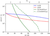Fig. 14. Comparison of the energy density we(ϑ) of the electrons and of the magnetic field wB(ϑ). The two additional (green) lines indicate the extension r68 for the synchrotron and for the inverse Compton component: the y-axes indicates the photon energy hν in units of eV (synchrotron, solid line) or GeV (IC, dash-dotted line).

Even though the nominal uncertainty on α is small (0.51 ± 0.0), the VHE spectral measurements show significant differences in the shape. The estimates of α therefore differ when using different sets of VHE measurements (see also Appendix A and Table A.1). An alternative combination of measurements that are consistent with each other (see also Appendix C) favours a significantly different value of $\check{\alpha }=0.{29}_{-0.06}^{+0.03}$. Without further data, it is impossible to determine whether these measurements exclude each other or whether the underlying systematic uncertainty on the shape of the energy spectrum is larger than estimated by the instrumental teams. The contemporaneous data taken during a flaring episode of the nebula are consistent with each other (see Table A.1). However, when looking at the temporal sequence of the observations (see Fig. A.1) it appears conceivable that the dynamical changes visible in the relevant part of the pulsar wind between the termination shock and the torus could be caused or accompanied by a change in the dissipation rate of magnetic field energy in the flow.

In addition to the disparity between the best-fitting values for α obtained with different VHE measurements (0.29…0.51), there is also a noticeable (but less significant) difference to the best-fitting value found for $\check{\alpha }=0.8_{-0.13}^{+0.16}$ in Sect. 4.4.1. For that fit, the spectral data from Fermi-LAT were used only– without including VHE data which covers the SED beyond the peak of the inverse-Compton component (see Sect. 4.4.2). In the context of the discussion related to the potential variability of the magnetic field configuration (see above) and the possible correlation with the hard X-ray flux (see Fig. A.1) it is clear that the value of 0.8 is too far off the range of values found with the VHE data to be explained by variability. Putting aside the possibility of systematic uncertainties, there remains as explanation that the model is missing an additional ingredient. Without attempting an additional fit here, a possible modification would be a more complicated model for the magnetic field strength and its variation in the nebula. An obvious modification could be applied to the radial dependence. The electrons contributing to the inverse Compton emission detected with Fermi-LAT are spatially more extended than the electrons radiating at VHE energies. In this sense, the value of α could smoothly change, steepening with increasing distance from a value of 0.5 to 1. In this way, a more accurate spectral measurement in the energy range covered with Fermi-LAT could establish a more detailed picture of the magnetic field distribution in the Crab Nebula.

6. Summary and conclusion

The observed broadband emission and spatial extension of the Crab Nebula have been used to reconstruct the contemporaneous properties of the relativistic electrons, magnetic field, and dust content in the pulsar wind nebula. The main findings can be summarised in the following points:

1. The assembled observational data for the Crab Nebula are unique as it covers an extremely broad energy range with an accuracy that is generally not appreciated when attempting to model the data.

2. The recent measurement of the spatial extension of the inverse Compton nebula provides insights into the magnetic field strength in the downstream region of the termination shock.

3. A detailed radiative model has been developed to estimate a minimal set of parameters related to the spatial and spectral distribution of electrons, dust, and the magnetic field under the assumption of radial symmetry.

4. The best-fitting model provides a good fit to the data. The χ² minimisation approach provides an accurate estimate of all the underlying parameters without degeneracies.

5. The VHE gamma-ray data provide the strongest constraint on the magnetic field strength beyond the termination shock at r_s: B(r) = B₀(r/r_s)^−α with $\check{\alpha }=0.51\pm 0.03$ and ${\check{B}}_0=(264\pm 9)\mathrm{\mu }\mathrm{G}$.

6. The long-standing assumption introduced about 50 years ago that the downstream magnetic field increases in a kinetically dominated pulsar wind (σ = 0.003) is ruled out by the data.

7. The downstream flow is dominated by magnetic energy density up to r ≈ 1.3r_s. For larger distances, the particle energy density dominates until equipartition is recovered in the periphery of the PWN.

8. VHE data taken during an increased hard X-ray flux state favour a value of $\check{\alpha }=0.{29}_{-0.05}^{+0.03}$, with an overall slightly worse goodness of fit.

9. The simultaneous fit of the synchrotron and dust emission provides an estimate of the total dust mass, temperature, and spatial distribution in the nebula. The resulting dust mass is approximately five times larger than previous estimates (De Looze et al. 2019). The larger dust mass increases the required efficiency for dust formation.

10. The production process of the two PeV photons detected from the Crab Nebula remains of uncertain origin. The simplest model would link the photon production to inverse Compton emission of PeV electrons which radiate 80–800 MeV synchrotron emission. Since the majority (> 75%)of this energetic synchrotron emission has been found to be produced in a compact region (Yeung & Horns 2020) with fast variability, the resulting constraint on the minimum (confining) magnetic field (> 500 μG) is in conflict with the comparably low value of magnetic field (≈85 μG) required to fit the inverse Compton and synchrotron emission simultaneously.

The results obtained here mainly rely on the assumptions of a spherical and static system. In principle, the model can be extended to axial symmetry and to include the effects of the flow in the radiative treatment. On the observational side, multi-instrument simultaneous VHE observations of the Crab Nebula are crucial to verify the effect of spectral variations. The upcoming spatially resolved observations of the X-ray polarisation of the Crab Nebula with the IXPE satellite (Weisskopf et al. 2016) will provide a measurement of the degree of small-scale turbulence in the flow (Bucciantini et al. 2017) which lead to a reduced fraction of polarised synchrotron emission.

Acknowledgments

Part of this work was supported by the German Deutsche Forschungsgemeinschaft, DFG project number 284334853: HO 3305/2 and by ANR-20-CE31-0010. This research has made use of NASA’s Astrophysics Data System Bibliographic Services. The authors thank the developers of matplotlib (Hunter 2007) for making their code available on a free and open-source basis. DH acknowledges support by the DFG under Germany’s Excellence Strategy – EXC 2121 “Quantum Universe” – 390833306. We thank the referee for the very useful reports and for encouraging us to investigate the differences found between the Fermi-LAT and VHE fit results.

References

Appendix A: Individual VHE data sets

The observation of VHE (E > 100 GeV) gamma-rays is the domain of ground based air shower detection. In this energy range, the Crab Nebula is the brightest steady source in the sky and therefore, the detection and observation of the Crab Nebula is the litmus test for VHE gamma-ray detectors. The fact that the very first TeV gamma-ray source clearly detected was the Crab Nebula (Weekes et al. 1989) underlines the importance of this particular source for ground based gamma-ray astronomy. The routine monitoring of this standard candle has lead to a large number of published data sets in this energy range with widely different detection techniques. We have selected observations which cover both a wide range of observation times (from 1997 to 2020) and different techniques (imaging air Cherenkov telescopes as well as shower front sampling with extended air shower arrays). This is not a complete collection but it is meant to provide a good cross section of the spectroscopic data from the past two decades.

The individual data sets are listed in Table A.1. The observational times as well as ranges of best-fitting values of α are included with the hard X-ray light curve from the nebula in Fig. A.1. The contemporaneous data sets are consistent within the uncertainties of α. When looking at the evolution of the hard X-ray flux and the changes of α, there is at least a trend visible: during higher flux states of hard X-rays, the VHE spectra tend to follow the shape given for a slower radial drop of the magnetic field. During lower flux states, the magnetic field seems to go down quicker with increasing distance.

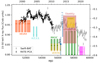Fig. A.1. Observed hard X-ray light curve (RXTE-PCA data from (Wilson-Hodge et al. 2011), Swift-BAT (Krimm et al. 2013) available through the BAT transient monitor page) from the Crab Nebula. The observed flux varies on time-scales of several years. The observations at VHE (listed in Table A.1) cover different parts of the X-ray flux states.

Appendix B: Pair-production opacity towards the Crab Nebula

The soft photon fields present in the Galactic disk include the cosmic microwave background (CMB) as well as dust and stellar emission. Energetic gamma-rays will be absorbed by pair-production processes when propagating in the soft photon background Gould & Schréder (1967). Using a recent radiation model of the Galaxy (Popescu et al. 2017), the optical depth for the line of sight towards the Crab Nebula is calculated to correct its apparent gamma-ray brightness for absorption (LHAASO Collaboration 2021). The CMB leads to a reduction by ≈24 % at E_γ = 2 PeV (assuming a distance of 2 kpc). At lower energies, the CMB photons are not sufficiently energetic to create pairs such that at E_γ = 100 TeV pairs are mainly produced with thermal dust emission. Given that the photon density of the dust emission is substantially smaller at the relevant wavelength of ≈100 μm, the resulting absorption is less pronounced than the CMB-related absorption at higher energies (1 − exp(−τ_γγ(E_γ = 100 TeV)) ≈ 1.5 %. However, the result on the opacity used by LHAASO Collaboration (2021) is not taking into account the anisotropy of the soft photon field.

Here, we provide an estimate of the previously neglected effect of anisotropy by using the following simplifications: (i) the relevant specific energy density λu_λ of the photon field is dominated by the dust component with a peak at λ ≈ 100 μm, (ii) the angular distribution of the anisotropic background field follows the measured local intensity, (iii) both, the intensity as well angular distribution remain constant along the line of sight towards the Crab Nebula.

The resulting optical depth τ_γγ(E_γ) for the Crab Nebula located at a distance d and in the direction along the normal vector e_C is given by:

$$\begin{array}{c}\hfill \tau (E_{\gamma })={\displaystyle \underset{0}{\overset{d}{\int }}\mathrm{d}x\underset{{\epsilon }_{\mathit{min}}}{\overset{{\epsilon }_{\mathit{max}}}{\int }}\mathrm{d}\epsilon n(\epsilon )\int \mathrm{d}\mathrm{\Omega }f({\mathbf{e}}_{\mathrm{\Omega }}){\sigma }_{\gamma \gamma }(s)(1-{\mathbf{e}}_{\mathrm{\Omega }}·{\mathbf{e}}_C),}\end{array}$$(B.1)

where σ_γγ is the pair production cross section (see e.g. Eq. 1 of Gould & Schréder (1967)), n(ε) is the total (sky integrated) differential number density of photons dn = n(ε)dεdV. The angular distribution f(e_Ω) was normalised over the entire sphere, such that:

$$\begin{array}{c}\hfill {\displaystyle \int }\mathrm{d}\mathrm{\Omega }f({\mathbf{e}}_{\mathrm{\Omega }})=1.\end{array}$$(B.2)

The unit vector e_Ω points towards a direction given in Galactic coordinates. This way, μ := e_Ω ⋅ e_C corresponds to the cosine of the angular distance between the photon directions of the gamma ray from the Crab Nebula and the soft photon from the Galactic background emission. The centre of momentum energy s depends on the photon energy E_γ, the soft photon’s energy ε as well as μ:

$$\begin{array}{c}\hfill s=2\epsilon E_{\gamma }(1-\mu ).\end{array}$$(B.3)

Following the approximation (i), the dust photon field was taken to be a single function

$$\begin{array}{c}\hfill n(\epsilon )=n_0{\left(\frac{\epsilon }{{\epsilon }_0}\right)}^{3.5}\frac{1}{exp(\epsilon /{\epsilon }_0)-1},\end{array}$$(B.4)

with n₀ = 1223.78 cm⁻³ eV⁻¹ and ε₀ = 1.7 × 10⁻³ eV. This is a reasonably close approximation of the model proposed by Popescu et al. (2017) around the peak at λ ≈ 100 μm.

The angular distribution at λ = 100 μm was taken from the all-sky map from DIRBE measurements (Schlegel et al. 1998) with the zodiacal foreground and point sources removed. In order to highlight the effect of the anisotropy, we calculated the optical depth for both cases (anisotropic and isotropic photon field) with the same energy density λu_λ and compare the results in Fig. B.1. While the simplified model reproduces well the more detailed calculation, taking additional photon fields as well as the spatial dependence of the photon density (Popescu et al. 2017) into account, the anisotropic case increases the attenuation as expected. At E_γ = 100 TeV, the flux is attenuated by about 3 % (as compared to about 1.7 % for the isotropic case). It is important to note, that this approach is particular to sources close to the Sun’s position, such that the approximations (ii) and (iii) allow the simplified treatment of the anisotropic case. The general anisotropic case has been treated in Porter et al. (2017) (and references therein).

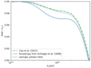Fig. B.1. Energy-dependent attenuation of gamma rays for the line of sight towards the Crab Nebula: The solid and dashed lines are the attenuation calculated here (see text for details) for the anisotropic radiation field (solid) and for the assumption of an isotropic radiation field with identical energy density (dashed line). The dash-dotted line is the attenuation as calculated in the framework of a detailed Galactic dust emission model, however assuming an isotropic radiation field (LHAASO Collaboration 2021)

Appendix C: Low α VHE solution

The combination of VHE data sets shown in Sect. 4.4.2 favours a value of α = 0.51 ± 0.03. However, the VHE data sets show individually quite different fitting results as demonstrated by the values in Table A.1. While there is a large number of possible combinations conceivable, there seems to be at least one additional combination of data sets that would favour a smaller value of α while still maintaining a good fit to the data. Excluding therefore the two data sets obtained with the H.E.S.S. telescopes which are not fit well by the model (see Table A.1), we combined the spectra measured with HEGRA, HAWC, and the Tibet ASγ experiments. The resulting estimate of $\alpha =0.{29}_{-0.06}^{+0.03}$ is significantly smaller than the value found for the data sets shown in Sect. 4.4.2.

The resulting fit (shown in Fig. C.1) is still acceptable with ${\chi }_{VHE}^2(dof)=30(32)$. The Tibet ASγ data requires an up-scaling of the energy scale (ζ = 1.07(2)) to match the model while in the case of the α = 0.51 fit, ζ = 0.92(2) (see Table C.1 for the results of this fit). The best-fitting parameters listed in Table C.2 are systematically different to the parameters listed for the solution with α = 0.51 (see Table 4). For the solution shown here, the magnetic field at the shock is smaller and drops off slower. To compensate, the spatial particle distribution does not extend as far as in the case of α = 0.51 (see parameters Ψ₃, Ψ₁₄). This in turn reduces the size of the IC nebula (see also Fig. 11). The resulting ${\chi }_{IC,ext}^2$ is therefore worse than in the solution with α = 0.51. Combined with the worse VHE fit, the probability to obtain this large value of χ²(dof) = 289(262) is only p(> χ², dof) = 0.12. Even though the goodness of fit is noticeably worse than in the α = 0.51 case, it is still acceptable.

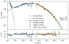Fig. C.1. When combining the energy spectra obtained with HEGRA, HAWC, and Tibet ASγ, the data-sets are consistent with each other (after scaling the energy) and can be described with the model reasonably well: ${\chi }_{VHE}^2(dof)=30(32)$.

Appendix D: UHE gamma-ray event statistic

In the main section, the expected number of events for the LHAASO observation (LHAASO Collaboration 2021) were used to compare with the observed number of events detected at PeV energies. The underlying calculation is performed using the exposure time (T_obs = 10⁷ s) and the collection areas listed in the published data¹⁰. The resulting event numbers N_i in bin i are calculated by integrating the differential photon flux predicted by the model Φ_model(E) within the bin interval E_i, low and E_i, high:

$$\begin{array}{c}\hfill N_i=T_{\mathrm{obs}}{A}_{eff,i}{\displaystyle \underset{E_{i,low}}{\overset{E_{i,high}}{\int }}}\mathrm{d}E{\mathrm{\Phi }}_{\mathit{model}}(E/\zeta )e^{-{\tau }_{\gamma \gamma }(E/\zeta )}.\end{array}$$(D.1)

In Tab. D.1, the resulting event numbers are compared with the background subtracted excess events from the data. For the two bins just below and above 1 PeV, the expected number of events is λ = 0.7 while the number of observed events (background free) is k = 2. The probability to observe 2 or more events is calculated with the Poissonian distribution

$$\begin{array}{c}\hfill p(k\ge 2)=1-p_{\lambda }(0)-p_{\lambda }(1)=1-exp(-\lambda )(1+\lambda )=15.6\%.\end{array}$$(D.2)

All Tables

All Figures

Fig. 1. Observed spectral energy distribution (SED) from radio to optical photon energies. The additional data from the recent compilation of photometric data from De Looze et al. (2019) are marked with white circles. Optical/UV data are presented with and without extinction correction (see text for more details). The SED has been fit with the superposition of thermal dust emission (see Table 3 for a list of parameters and uncertainties) and the underlying synchrotron continuum (see Table 4).

In the text

Fig. 2. Predicted and observed optical spectra of the Crab Nebula. In concentric annuli, the mean and root mean square of the spectral indices sO (Iν ∝ ν−sO) have been determined from the data displayed in Fig. 1 of Véron-Cetty & Woltjer (1993). The superimposed curve is calculated from the intensity expected from the synchrotron model as described in Sect. 4.3 with the best-fitting parameters listed in Table 4. It is important to note that these data have not been used in the fit.

In the text

Fig. 3. SED of the Crab Nebula centred on the X-ray energy range. The best-fitting model (blue line, see details on the fitting procedure in Sect. 4 and Table 4) is shown along with measurements from different X-ray observatories. The normalisation of the spectrum measured with XMM-Newton (yellow band) has been scaled up by 16% to be consistent with the absolute flux measurement with NuSTAR (magenta band). The COMPTEL gamma-ray flux has been scaled up by 30% to match the extrapolation of the SPI spectrum.

In the text

	Fig. 4. Electron number density nel, as a function of γ for different values of the distance to the centre of the Crab Nebula r and the volume average. The parameters used here are listed in Table 4.
In the text

Fig. 5. Results of the fitting procedure. Left column: (a) $\mathrm{\Delta }{\chi }_{\text{sync}}^2(\alpha ,B_0)$ and (c) $\mathrm{\Delta }{\chi }_{\text{sync}}^2(\alpha )$. Right column: (b) $\mathrm{\Delta }{\log }_{10}({\chi }_{\text{IC}}^2(\alpha ,B_0)+1)$ and (d) ${\log }_{10}(\mathrm{\Delta }{\chi }_{\text{IC}}^2(\alpha )+1)$. In the top panels, for each combination of α, B0, the other parameters of the model are marginalised; in the bottom panels, this includes B0. The dotted white lines in the top panels indicate the contours for constant values of volume averaged ⟨B⟩ = 30, 60, 90 μG. The cyan dashed line indicates the combinations B0 and α with the minimum total energy Wtot in electrons and magnetic field. The yellow solid contour marks the 95% confidence level error box for B0, α. The grey boxes in the bottom panel indicate the 95% confidence interval for α. In the bottom right diagram, the cyan dashed line indicates the minimal total energy Wtot for a given α. For a discussion on the relevance of the co-location of the global minimum ${\chi }_{\text{IC}}^2$ with the corresponding global minimum of Wtot, see the text.

In the text

Fig. 6. Volume-integrated total energy Wtot equals the sum of the energy in relativistic electrons We and magnetic field WB. For any best-fitting set of parameters, the energy partition is a function of the normalisation B0 of the magnetic field at the shock distance rs. The best-fitting value is found to be $\check{B_0}=(497\pm 43)\mathrm{\mu }\mathrm{G}$ (90% c.l. uncertainty, including systematical uncertainties). This value is slightly smaller than the minimal energy configuration at B0 = 514 μG.

In the text

Fig. 7. Best-fitting model in comparison to the data. The upper plot shows the synchrotron and inverse Compton (IC) radiation by radio (R) and wind (W) electrons produced in the spatially varying magnetic field and seed photon field (blue and magenta coloured broken lines indicate the contributions from IC scattering on individual seed photon fields). The blue data points are used in the fit to determine the parameters ${\check{\mathrm{\Psi }}}_{1\dots 20}$ listed in Table 4. The VHE data have been scaled using the values of ζi determined for each data-set (see text for further details) to adjust the energy scale for prediction given by the global minimum ${\chi }^2(\check{\alpha }=0.51)$. In the lower plot, the relative residuals are shown (statistical uncertainties only).

In the text

	Fig. 8. Comparison of the best-fitting model with the HE and VHE data. The detailed view confirms the consistency of the selected data sets (after scaling) and the good agreement of the model to the data. The selected VHE data sets overlap with the LAT data and each data set overlaps with at least one other VHE data set.
In the text

	Fig. 9. Extension of the model emission is characterised by the radial size θ68. The model curve is the calculated extension which matches well the observational data.
In the text

Fig. 10. Overall spectral energy distribution for the estimated best-fitting parameters ${\check{\mathrm{\Psi }}}_{1\cdots 20}$ (after minimising ${\chi }_{\text{IC}}^2$ for fixed values of α) is shown. The value of α characterises the radial decrease of the magnetic field B ∝ r−α (see Eq. (14)). While the synchrotron part of the spectral energy distribution is almost degenerate with respect to the choice of α, the inverse Compton dominated part (right panel) shows noticeable differences up to the peak at approximately 1011 eV. Note, in the left panel the sum of synchrotron and inverse Compton emission is shown, while in the right panel, the SED of the inverse Compton emission is additionally superimposed.

In the text

Fig. 11. Angular extension from the fitting procedure described in the text. After marginalising ${\check{\mathrm{\Psi }}}_{1\cdots 20}$, the predicted angular extension of the synchrotron nebula matches the data well for values of α = 0, …, 1.1 with very small variations visible in the transition between thermal and non-thermal emission at near- to far infrared. At higher energies, the predicted size differs mostly at the low-energy end of the inverse Compton emission.

In the text

Fig. 12. A suggested model for the SED including a secondary electron contribution located at the shock position. The low and high state spectra as measured with Fermi-LAT are shown for comparison (Yeung & Horns 2020). The secondary electrons’ spectrum during average (high) state is a power-law with dn/dγ ∝ γ−2.3 between γ1 = 3 × 109 and γ2 = 7(18)×109. The magnetic field in the region is chosen to be 85 μG. The total energy content of the electrons is 2(3)×1042 ergs. The dotted lines indicate the effect of absorption on the Galactic foreground emission (see also Appendix B).

In the text

Fig. 13. Energy density of the seed photons as a function of the distance from the pulsar. The dust emissivity was modelled to be confined in a shell surrounding the optical nebula. As a comparison, a composite of X-ray (Chandra: blue, white)/optical(HST: purple)/ infrared (Spitzer: pink) composite image from the nebula is shown with approximately matching spatial scale. Background image credit: X-ray: NASA/CXC/SAO; Optical: NASA/STScI; Infrared: NASA-JPL-Caltech).

In the text

	Fig. 14. Comparison of the energy density we(ϑ) of the electrons and of the magnetic field wB(ϑ). The two additional (green) lines indicate the extension r68 for the synchrotron and for the inverse Compton component: the y-axes indicates the photon energy hν in units of eV (synchrotron, solid line) or GeV (IC, dash-dotted line).
In the text

	Fig. A.1. Observed hard X-ray light curve (RXTE-PCA data from (Wilson-Hodge et al. 2011), Swift-BAT (Krimm et al. 2013) available through the BAT transient monitor page) from the Crab Nebula. The observed flux varies on time-scales of several years. The observations at VHE (listed in Table A.1) cover different parts of the X-ray flux states.
In the text

Fig. B.1. Energy-dependent attenuation of gamma rays for the line of sight towards the Crab Nebula: The solid and dashed lines are the attenuation calculated here (see text for details) for the anisotropic radiation field (solid) and for the assumption of an isotropic radiation field with identical energy density (dashed line). The dash-dotted line is the attenuation as calculated in the framework of a detailed Galactic dust emission model, however assuming an isotropic radiation field (LHAASO Collaboration 2021)

In the text

	Fig. C.1. When combining the energy spectra obtained with HEGRA, HAWC, and Tibet ASγ, the data-sets are consistent with each other (after scaling the energy) and can be described with the model reasonably well: ${\chi }_{VHE}^2(dof)=30(32)$.
In the text

References

- Abdalla, H., Aharonian, F., Ait Benkhali, F., et al. 2020, Nat. Astron., 4, 167 [NASA ADS] [CrossRef] [Google Scholar]
- Abdo, A. A., Ackermann, M., Ajello, M., et al. 2009, Phys. Rev. Lett., 102, 181101 [NASA ADS] [CrossRef] [Google Scholar]
- Abdo, A. A., Ackermann, M., Ajello, M., et al. 2011, Science, 331, 739 [NASA ADS] [CrossRef] [Google Scholar]
- Abeysekara, A. U., Albert, A., Alfaro, R., et al. 2019, ApJ, 881, 134 [NASA ADS] [CrossRef] [Google Scholar]
- Ackermann, M., Ajello, M., Allafort, A., et al. 2012, Astropart. Phys., 35, 346 [Google Scholar]
- Aharonian, F., Akhperjanian, A., Beilicke, M., et al. 2004, ApJ, 614, 897 [NASA ADS] [CrossRef] [Google Scholar]
- Aharonian, F., Akhperjanian, A. G., Bazer-Bachi, A. R., et al. 2006, A&A, 457, 899 [NASA ADS] [CrossRef] [EDP Sciences] [Google Scholar]
- Aharonian, F. A., Kelner, S. R., & Prosekin, A. Y. 2010, Phys. Rev. D., 82, 043002 [NASA ADS] [CrossRef] [Google Scholar]
- Aleksić, J., Ansoldi, S., Antonelli, L. A., et al. 2015, J. High Energy Astrophys., 5, 30 [Google Scholar]
- Aliu, E., Archambault, S., Aune, T., et al. 2014, ApJ, 781, L11 [Google Scholar]
- Amenomori, M., Bao, Y. W., Bi, X. J., et al. 2019, Phys. Rev. Lett., 123, 051101 [NASA ADS] [CrossRef] [Google Scholar]
- Atoyan, A. M., & Aharonian, F. A. 1996, MNRAS, 278, 525 [NASA ADS] [Google Scholar]
- Band, D., Matteson, J., Ford, L., et al. 1993, ApJ, 413, 281 [Google Scholar]
- Bietenholz, M. F., & Kronberg, P. P. 1990, ApJ, 357, L13 [NASA ADS] [CrossRef] [Google Scholar]
- Bietenholz, M. F., Hester, J. J., Frail, D. A., & Bartel, N. 2004, ApJ, 615, 794 [NASA ADS] [CrossRef] [Google Scholar]
- Blair, W. P., Long, K. S., Vancura, O., et al. 1992, ApJ, 399, 611 [NASA ADS] [CrossRef] [Google Scholar]
- Bohren, C., & Huffman, D. R. 1998, in Absorption and Scattering of Light by Small Particles, eds. C. Bohren, & D. R. Huffman (Wiley Science Paperback Series) [CrossRef] [Google Scholar]
- Bucciantini, N., Bandiera, R., Olmi, B., & Del Zanna, L. 2017, MNRAS, 470, 4066 [CrossRef] [Google Scholar]
- Buehler, R., Scargle, J. D., Blandford, R. D., et al. 2012, ApJ, 749, 26 [NASA ADS] [CrossRef] [Google Scholar]
- Čadež, A., Carramiñana, A., & Vidrih, S. 2004, ApJ, 609, 797 [CrossRef] [Google Scholar]
- Crusius, A., & Schlickeiser, R. 1986, A&A, 164, L16 [NASA ADS] [Google Scholar]
- de Jager, O. C., & Harding, A. K. 1992, ApJ, 396, 161 [NASA ADS] [CrossRef] [Google Scholar]
- De Looze, I., Barlow, M. J., Bandiera, R., et al. 2019, MNRAS, 488, 164 [NASA ADS] [CrossRef] [Google Scholar]
- Feng, H., Li, H., Long, X., et al. 2020, Nat. Astron., 4, 511 [CrossRef] [Google Scholar]
- Gomez, H. L., Krause, O., Barlow, M. J., et al. 2012, ApJ, 760, 96 [NASA ADS] [CrossRef] [Google Scholar]
- Gould, R. J., & Schréder, G. P. 1967, Phys. Rev., 155, 1404 [Google Scholar]
- Green, G. M., Schlafly, E., Zucker, C., Speagle, J. S., & Finkbeiner, D. 2019, ApJ, 887, 93 [NASA ADS] [CrossRef] [Google Scholar]
- Greiveldinger, C., & Aschenbach, B. 1999, ApJ, 510, 305 [NASA ADS] [CrossRef] [Google Scholar]
- Hennessy, G. S., O’Connell, R. W., Cheng, K. P., et al. 1992, ApJ, 395, L13 [NASA ADS] [CrossRef] [Google Scholar]
- H. E. S. S. Collaboration (Abdalla, H., et al.) 2020, Nat. Astron., 4, 167 [NASA ADS] [CrossRef] [Google Scholar]
- H. E. S. S. Collaboration (Abramowski, A., et al.) 2014, A&A, 562, L4 [NASA ADS] [CrossRef] [EDP Sciences] [Google Scholar]
- Hickson, P., & van den Bergh, S. 1990, ApJ, 365, 224 [NASA ADS] [CrossRef] [Google Scholar]
- Hillas, A. M., Akerlof, C. W., Biller, S. D., et al. 1998, ApJ, 503, 744 [NASA ADS] [CrossRef] [Google Scholar]
- Holler, M. 2014, PhD Thesis, Universität Potsdam, Germany [Google Scholar]
- Holler, M., Berge, D., van Eldik, C., et al. 2015, ArXiv e-prints [arXiv:1509.02902] [Google Scholar]
- Horns, D., Aharonian, F., Santangelo, A., Hoffmann, A. I. D., & Masterson, C. 2006, A&A, 451, L51 [NASA ADS] [CrossRef] [EDP Sciences] [Google Scholar]
- Hunter, J. D. 2007, Comput. Sci. Eng., 9, 90 [NASA ADS] [CrossRef] [Google Scholar]
- Jones, F. C. 1968, Phys. Rev., 167, 1159 [NASA ADS] [CrossRef] [Google Scholar]
- Jourdain, E., & Roques, J. P. 2009, ApJ, 704, 17 [Google Scholar]
- Jourdain, E., & Roques, J. P. 2020, ApJ, 899, 131 [NASA ADS] [CrossRef] [Google Scholar]
- Kennel, C. F., & Coroniti, F. V. 1984, ApJ, 283, 694 [CrossRef] [Google Scholar]
- Khangulyan, D., Arakawa, M., & Aharonian, F. 2020, MNRAS, 491, 3217 [NASA ADS] [CrossRef] [Google Scholar]
- Kirsch, M. G., Briel, U. G., Burrows, D., et al. 2005, SPIE Conf. Ser., 5898, 22 [NASA ADS] [Google Scholar]
- Komissarov, S. S., & Lyubarsky, Y. E. 2003, MNRAS, 344, L93 [NASA ADS] [CrossRef] [Google Scholar]
- Krimm, H. A., Holland, S. T., Corbet, R. H. D., et al. 2013, ApJS, 209, 14 [NASA ADS] [CrossRef] [Google Scholar]
- Kuiper, L., Hermsen, W., Cusumano, G., et al. 2001, A&A, 378, 918 [NASA ADS] [CrossRef] [EDP Sciences] [Google Scholar]
- LHAASO Collaboration (Cao, Z., et al.) 2021, Science, 373, 425 [Google Scholar]
- Ling, J. C., & Wheaton, W. A. 2003, ApJ, 598, 334 [NASA ADS] [CrossRef] [Google Scholar]
- Liu, R.-Y., & Wang, X.-Y. 2021, ApJ, 922, 221 [NASA ADS] [CrossRef] [Google Scholar]
- Lobanov, A. P., Horns, D., & Muxlow, T. W. B. 2011, A&A, 533, A10 [NASA ADS] [CrossRef] [EDP Sciences] [Google Scholar]
- Luo, Y., Lyutikov, M., Temim, T., & Comisso, L. 2020, ApJ, 896, 147 [NASA ADS] [CrossRef] [Google Scholar]
- Lyutikov, M., Temim, T., Komissarov, S., et al. 2019, MNRAS, 489, 2403 [NASA ADS] [CrossRef] [Google Scholar]
- Madsen, K. K., Reynolds, S., Harrison, F., et al. 2015, ApJ, 801, 66 [Google Scholar]
- Madsen, K. K., Forster, K., Grefenstette, B. W., Harrison, F. A., & Stern, D. 2017, ApJ, 841, 56 [NASA ADS] [CrossRef] [Google Scholar]
- Madsen, K. K., Burwitz, V., Forster, K., et al. 2021, ArXiv e-prints [arXiv:2111.01613] [Google Scholar]
- MAGIC Collaboration (Acciari, V. A., et al.) 2020, A&A, 635, A158 [NASA ADS] [CrossRef] [EDP Sciences] [Google Scholar]
- Marsden, P. L., Gillett, F. C., Jennings, R. E., et al. 1984, ApJ, 278, L29 [NASA ADS] [CrossRef] [Google Scholar]
- Martín, J., Torres, D. F., & Rea, N. 2012, MNRAS, 427, 415 [NASA ADS] [CrossRef] [Google Scholar]
- Mayer, M., Buehler, R., Hays, E., et al. 2013, ApJ, 775, L37 [NASA ADS] [CrossRef] [Google Scholar]
- Meagher, K.& VERITAS Collaboration 2016, Proc. 34th International Cosmic Ray Conference (ICRC2015), 30 July - 6 August, 2015, The Hague, The Netherlands, online at http://pos.sissa.it/cgi-bin/reader/conf.cgi?confid=236, 792 [Google Scholar]
- Meyer, M., Horns, D., & Zechlin, H.-S. 2010, A&A, 523, A2 [NASA ADS] [CrossRef] [EDP Sciences] [Google Scholar]
- Mori, K., Burrows, D. N., Hester, J. J., et al. 2004, ApJ, 609, 186 [NASA ADS] [CrossRef] [Google Scholar]
- O’Donnell, J. E. 1994, ApJ, 422, 158 [Google Scholar]
- Owen, P. J., & Barlow, M. J. 2015, ApJ, 801, 141 [NASA ADS] [CrossRef] [Google Scholar]
- Pacini, F., & Salvati, M. 1973, ApJ, 186, 249 [NASA ADS] [CrossRef] [Google Scholar]
- Peng, Q.-Y., Bao, B.-W., Lu, F.-W., & Zhang, L. 2022, ApJ, 926, 7 [NASA ADS] [CrossRef] [Google Scholar]
- Planck Collaboration XXVI. 2016, A&A, 594, A26 [NASA ADS] [CrossRef] [EDP Sciences] [Google Scholar]
- Popescu, C. C., Yang, R., Tuffs, R. J., et al. 2017, MNRAS, 470, 2539 [NASA ADS] [CrossRef] [Google Scholar]
- Porter, T. A., Jóhannesson, G., & Moskalenko, I. V. 2017, ApJ, 846, 67 [NASA ADS] [CrossRef] [Google Scholar]
- Porth, O., Komissarov, S. S., & Keppens, R. 2013, MNRAS, 438, 278 [NASA ADS] [CrossRef] [Google Scholar]
- Rees, M. J., & Gunn, J. E. 1974, MNRAS, 167, 1 [CrossRef] [Google Scholar]
- Ritacco, A., Macías-Pérez, J. F., Ponthieu, N., et al. 2018, A&A, 616, A35 [NASA ADS] [CrossRef] [EDP Sciences] [Google Scholar]
- Rudy, A., Horns, D., DeLuca, A., et al. 2015, ApJ, 811, 24 [NASA ADS] [CrossRef] [Google Scholar]
- Schlegel, D. J., Finkbeiner, D. P., & Davis, M. 1998, ApJ, 500, 525 [Google Scholar]
- Shaposhnikov, N., Jahoda, K., Markwardt, C., Swank, J., & Strohmayer, T. 2012, ApJ, 757, 159 [NASA ADS] [CrossRef] [Google Scholar]
- Shibata, S., Tomatsuri, H., Shimanuki, M., Saito, K., & Mori, K. 2003, MNRAS, 346, 841 [CrossRef] [Google Scholar]
- Smith, N. 2003, MNRAS, 346, 885 [CrossRef] [Google Scholar]
- Strong, A., & Collmar, W. 2019, Mem. Soc. Astron. Ital., 90, 297 [Google Scholar]
- Strüder, L., Briel, U., Dennerl, K., et al. 2001, A&A, 365, L18 [Google Scholar]
- Tanaka, S. J., & Asano, K. 2017, ApJ, 841, 78 [NASA ADS] [CrossRef] [Google Scholar]
- Tanaka, S. J., Toma, K., & Tominaga, N. 2018, MNRAS, 478, 4622 [NASA ADS] [CrossRef] [Google Scholar]
- Tavani, M., Bulgarelli, A., Vittorini, V., et al. 2011, Science, 331, 736 [CrossRef] [PubMed] [Google Scholar]
- Temim, T., & Dwek, E. 2013, ApJ, 774, 8 [NASA ADS] [CrossRef] [Google Scholar]
- Temim, T., Gehrz, R. D., Woodward, C. E., et al. 2006, AJ, 132, 1610 [NASA ADS] [CrossRef] [Google Scholar]
- Tomsick, J., & COSI Collaboration 2022, 37th International Cosmic Ray Conference, 12-23 July 2021, Berlin, Germany, online at https://pos.sissa.it/cgi-bin/reader/conf.cgi?confid=395, 652 [Google Scholar]
- Toor, A., & Seward, F. D. 1974, AJ, 79, 995 [Google Scholar]
- Trimble, V. 1973, PASP, 85, 579 [NASA ADS] [CrossRef] [Google Scholar]
- Tsujimoto, M., Guainazzi, M., Plucinsky, P. P., et al. 2011, A&A, 525, A25 [NASA ADS] [CrossRef] [EDP Sciences] [Google Scholar]
- Véron-Cetty, M. P., & Woltjer, L. 1993, A&A, 270, 370 [Google Scholar]
- Weekes, T. C., Cawley, M. F., Fegan, D. J., et al. 1989, ApJ, 342, 379 [NASA ADS] [CrossRef] [Google Scholar]
- Weiland, J. L., Odegard, N., Hill, R. S., et al. 2011, ApJS, 192, 19 [Google Scholar]
- Weisskopf, M. C., Silver, E. H., Kestenbaum, H. L., Long, K. S., & Novick, R. 1978, ApJ, 220, L117 [NASA ADS] [CrossRef] [Google Scholar]
- Weisskopf, M. C., Guainazzi, M., Jahoda, K., et al. 2010, ApJ, 713, 912 [Google Scholar]
- Weisskopf, M. C., Elsner, R. F., Kolodziejczak, J. J., O’Dell, S. L., & Tennant, A. F. 2012, ApJ, 746, 41 [NASA ADS] [CrossRef] [Google Scholar]
- Weisskopf, M. C., Tennant, A. F., Arons, J., et al. 2013, ApJ, 765, 56 [NASA ADS] [CrossRef] [Google Scholar]
- Weisskopf, M. C., Ramsey, B., O’Dell, S., et al. 2016, SPIE Conf. Ser., 9905, 990517 [NASA ADS] [Google Scholar]
- Wells, R. M. 2019, PhD Thesis, Iowa State University, Graduate Theses and Dissertations, 1706 [Google Scholar]
- Wilson-Hodge, C. A. 2012, When a Standard Candle Flickers: Crab NebulaVariations in Hard X-rays, Tech. rep., Nasa Marshall Space Flight Center Huntsville, USA [Google Scholar]
- Wilson-Hodge, C. A., Cherry, M. L., Case, G. L., et al. 2011, ApJ, 727, L40 [Google Scholar]
- Woosley, S. E., & Weaver, T. A. 1995, ApJS, 101, 181 [Google Scholar]
- Yeung, P. K. H., & Horns, D. 2019, ApJ, 875, 123 [NASA ADS] [CrossRef] [Google Scholar]
- Yeung, P. K. H., & Horns, D. 2020, A&A, 638, A147 [NASA ADS] [CrossRef] [EDP Sciences] [Google Scholar]
- Zubko, V. G., Mennella, V., Colangeli, L., & Bussoletti, E. 1996, MNRAS, 282, 1321 [Google Scholar]