| Issue |
A&A
Volume 670, February 2023
|
|
|---|---|---|
| Article Number | A42 | |
| Number of page(s) | 12 | |
| Section | Planets and planetary systems | |
| DOI | https://doi.org/10.1051/0004-6361/202244347 | |
| Published online | 03 February 2023 | |
L 363-38 b: A planet newly discovered with ESPRESSO orbiting a nearby M dwarf star
1
ETH Zurich, Institute for Particle Physics and Astrophysics,
Wolfgang-Pauli-Strasse 27,
8093
Zurich, Switzerland
e-mail: This email address is being protected from spambots. You need JavaScript enabled to view it.
2
Département d’Astronomie, Université de Genève,
Chemin Pegasi 51,
1290
Versoix, Switzerland
3
Space Research Institute, Austrian Academy of Sciences,
Schmiedlstr. 6,
8042
Graz, Austria
Received:
24
June
2022
Accepted:
25
October
2022
Abstract
Context. Planets around stars in the solar neighbourhood will be prime targets for characterisation with upcoming large space- and ground-based facilities. Since large-scale exoplanet searches will not be feasible with such telescopes, it is crucial to use currently available data and instruments to find possible target planets before next-generation facilities come online.
Aims. We aim to detect new extrasolar planets around stars in the solar neighbourhood via blind radial velocity (RV) searching with ESPRESSO. Our target sample consists of nearby stars (d < 11 pc) with few (<10) or no previous RV measurements.
Methods. We used 31 radial velocity measurements obtained with ESPRESSO at the VLT between December 2020 and February 2022 of the nearby M dwarf star (M★ = 0.21 M⊙, d = 10.23 pc) L 363-38 to derive the orbital parameters of the newly discovered planet. In addition, we used TESS photometry and archival VLT/NaCo high-contrast imaging data to put further constraints on the orbit inclination and the possible planetary system architecture around L 363-38.
Results. We present the detection of a new extrasolar planet orbiting the nearby M dwarf star L 363-38. L 363-38 b is a planet with a minimum mass of mp sin(i) = 4.67 ± 0.43 M⊕ orbiting its star with a period of P = 8.781 ± 0.007 days, corresponding to a semi-major axis of a = 0.048 ± 0.006 AU, which is smaller than the inner edge of the habitable zone. We further estimate a minimum radius of rp sin(i) ≈ 1.55–2.75 R⊕ and an equilibrium temperature of Teq ≈ 330 K.
Conclusions. With this study, we further demonstrate the potential of the state-of-the-art spectrograph ESPRESSO in detecting and investigating planetary systems around nearby M dwarf stars, which were inaccessible to previous instruments such HARPS.
Key words: planets and satellites: detection / techniques: radial velocities / planets and satellites: fundamental parameters / stars: individual: L 363-38
© The Authors 2023
 Open Access article, published by EDP Sciences, under the terms of the Creative Commons Attribution License (https://creativecommons.org/licenses/by/4.0), which permits unrestricted use, distribution, and reproduction in any medium, provided the original work is properly cited.
This article is published in open access under the Subscribe-to-Open model. This email address is being protected from spambots. You need JavaScript enabled to view it. to support open access publication.
1 Introduction
In the last decades, the growing interest in exoplanet science, as well as technical developments, have led to the discovery of over 5000 exoplanets orbiting stars up to thousands of pc. However, a complete census of the planets in the solar neighbourhood (d < 15 pc) is still lacking. Such planets will be the prime targets for characterisation with new and upcoming space- and ground-based facilities such as the James Webb Space Telescope (JWST, Gardner et al. 2006), the Enhanced Resolution Imager and Spec-trograph (ERIS, Davies et al. 2018) at the Very Large Telescope (VLT), the Mid-infrared ELT Imager and Spectrograph (METIS, Quanz et al. 2015; Brandl et al. 2021), and the ArmazoNes high Dispersion Echelle Spectrograph (ANDES, formerly known as High Resolution Echelle Spectrograph, HIRES, Marconi et al. 2016) at the Extremely Large Telescope (ELT), and, especially, for future space missions such as the Habitable Exoplanet Observatory (HabEx, Gaudi et al. 2020), the Large UV/Optical/IR Surveyor (LUVOIR, Peterson et al. 2017; The LUVOIR Team 2019), the Large Interferometer for Exoplanets (LIFE, Quanz et al. 2018, 2022; Konrad et al. 2022; Dannert et al. 2022; Alei et al. 2022), and the Closeby Habitable Exoplanet Survey (CHES, Ji et al. 2022), whose goal is to characterise Earth-like planets around the nearest stars. Since large-scale exoplanet searches will not be feasible with such telescopes, or at least not cheaply, it is crucial to use currently available data and instruments to find possible target planets (or a lack thereof) in the solar neighbourhood before next-generation facilities come online.
To determine the current constraints on the planet population in the solar neighbourhood and to prioritise targets for these upcoming instruments and missions, we started a project to systematically search for planets and substellar companions around nearby stars (d < 15 pc), mostly using the high-contrast imaging (HCI) and radial velocity (RV) techniques. This programme consists of re-analysing archival direct imaging data (e.g. Boehle et al. 2019) as well as proposing new observations. In this paper we concentrate on new radial velocity data obtained with the Echelle SPectrograph for Rocky Exoplanets and Stable Spectroscopic Observations (ESPRESSO, Pepe et al. 2021; González Hernández et al. 2018). ESPRESSO is the state-of-the-art, ultra-stable, high-resolution spectrograph installed at the VLT, with a resolving power of R ~ 140000 covering the spectral range from ~380 nm to ~788 nm. In the best observing conditions, ESPRESSO is able to reach a precision at the level of ~ 10 cm s−1 on the sky, which would allow us to detect Earth-like planets around Sun-like stars. This is one order of magnitude better than its predecessor, the High Accuracy Radial velocity Planet Searcher (HARPS, Pepe et al. 2002; Mayor et al. 2003). ESPRESSO can collect light from either a single VLT Unit Telescope (UT) or up to four UTs simultaneously through the Coudé trains (Cabral et al. 2010), allowing for high-cadence RV observations. Additional information about the ESPRESSO instrument is available in the ESO user manual and documentation1. Since the start of operations in 2018, ESPRESSO has proved successful in both discovering new planets (Lillo-Box et al. 2021; Faria et al. 2022) and better constraining the properties of known planetary systems (e.g. Toledo-Padrón et al. 2020; Damasso et al. 2020; Mortier et al. 2020; Suárez Mascareño et al. 2020; Sozzetti et al. 2021; Leleu et al. 2019, Leleu et al. 2021; Jordán et al. 2022).
In the following, we report the detection and characterisation of a planet orbiting the nearby M dwarf star L 363-38. This is one of the few standalone planet discoveries with ESPRESSO so far. The observations are described in Sect. 2. In Sect. 3, we report the stellar parameters and describe the performed analysis. The results are discussed in Sect. 4, and we conclude in Sect. 5.
Summary of radial velocity observations.
2 Observations
2.1 Radial velocities
L 363-38 was observed using ESPRESSO at the VLT between December 12, 2020 and February 08, 2022 as part of a monitoring program of nearby (d < 11 pc) stars with few (<10) or no previous RV measurements (programme ID 106.21BN.001 with carry over during P108, PI Anna Boehle). Throughout the two observing periods we obtained a total of 31 observations (7 during P106 and 24 during P108) with a median observing cadence of 2.1 days. Every spectrum was obtained with a 15 min integration time plus 10 min of telescope and instrument overhead, resulting in 25 min of telescope time per RV measurement. For this source, eight previous RV measurements obtained with HARPS between August 7, 2003, and December 8, 2010, are also available. Since the HARPS observations have lower significance levels compared to the ESPRESSO ones, in this paper we only discuss the analysis of the ESPRESSO radial velocities. However, we checked that these results are consistent with the ones obtained including the HARPS observations. Details about all RV observations are given in Tables 1 and A.1.
The radial velocity data used in this work were processed and partly analysed using the Data & Analysis Center for Exoplanets (DACE), a facility dedicated to extrasolar planets data visualisation, exchange and analysis hosted by the University of Geneva2. Specifically, we downloaded the RV time series using the DACE python APIs and analysed them using the dedicated modules kepmodel (Delisle et al. 2016, Delisle et al. 2020a,b), samsam (Haario et al. 2001; Andrieu & Thoms 2008; Delisle et al. 2018); spleaf (Foreman-Mackey et al. 2017; Delisle et al. 2020b, Delisle et al. 2022; Gordon et al. 2020), and kepderiv, which allow advanced statistical methods to model the Keplerian motion of planets and disentangle it from stellar activity signals. The RV and stellar activity indicators provided in DACE are computed by cross-correlating the calibrated spectra with stellar templates for the specific stellar class, using the publicly-available ESPRESSO Data Reduction Software3.
2.2 TESS photometry
L 363-38 (TIC 118585685) was observed by the Transiting Exoplanet Survey Satellite (TESS, Ricker et al. 2015) during Cycle 1 (Sector 2, August 23–September 20, 2018) and Cycle 3 (Sector 29, August 26–September 21, 2020). In order to investigate potential transits, we retrieved the 2-min cadence Presearch Data Conditioning (PDC) light curves (Smith et al. 2012; Stumpe et al. 2014) from the TESS Science Processing Operations Center (Jenkins et al. 2016).
2.3 High-contrast imaging
L 363-38 was observed with the NAOS-CONICA instrument at the VLT (NaCo, Lenzen et al. 2003; Rousset et al. 2003) between December 07, 2003 and December 10, 2003 as part of a survey aimed at constraining stellar multiplicity at very low masses (programme ID 072.C-0570A, PI J.-L. Beuzit). The observations were obtained with the narrow-band infrared filter NB_1.64 (λ0 = 1.644 μm, Δλ = 0.018 μm) in imaging mode for a total observing time of 160 s. We downloaded the raw files from the ESO archive, and we reduced and analysed them with the state-of-the-art, direct-imaging data pipeline PynPoint (Amara & Quanz 2012; Stolker et al. 2019).
3 Analysis
3.1 Stellar properties
L 363-38 (also known as LHS 1134 and GJ 3049, among others) is a high, proper-motion, nearby M4 star (Gaidos et al. 2014). The parallax reported in the Gaia Data Release 3 (DR3, Gaia Collaboration 2016, Gaia Collaboration 2021; Babusiaux et al. 2023), π = 97.660 ± 0.032 mas, corresponds to a distance of d = 10.232 ± 0.008 pc. The apparent V-band magnitude is V = 11.51 mag, which, assuming the bolometric correction for M-type stars from Habets & Heintze (1981) and the distance above, corresponds to a bolometric luminosity of L★ = 0.013 L⊙. The Gaia DR3 provides an effective temperature of Teff = 3129 K and a surface gravity log g = 4.97 dex. Its stellar mass is M⊙ = 0.21 ± 0.014 M⊙ (Winters et al. 2021 and references therein). Maldonado et al. (2020) provided a stellar age of 8.07 ± 4.12 Gyr. We further checked that the star is not in a binary system by comparing the significance of the excess noise in the Gaia DR2 (Gaia Collaboration 2018; Arenou et al. 2018; Lindegren et al. 2018) astrometric fit (D) to the distribution of this parameter for a volume limited sample of M stars with d < 11 pc, and that it is not listed as a double or multiple system in the HIPPARCOS catalogue (Esa 1997). Vrijmoet et al. (2020) found some perturbation in the astrometric residual, which may indicate the presence of a companion, but with the available data they were not able to confirm and characterise it. We also checked that, although Gaia DR3 provides a RUWE of 1.36, the source is not labelled as a non-single star in the Gaia DR3. The general properties of L 363-38 are listed in Table 2.
Stellar properties of L 363-38.
3.2 Radial velocities
The RV time series from the ESPRESSO observations are shown in Fig. 1 (left). In addition, Fig. 2 shows the generalised Lomb-Scargle periodogram (Cumming et al. 2008, with formalism from Zechmeister & Kürster 2009) of the ESPRESSO RV and of some stellar activity indicators: full width at half maximum (FWHM) of the cross-correlation function (CCF), CCF contrast and bis-span, and Log(R′/HK). The RV periodogram shows a clear peak at P = 8.781 days and its 1 (sideral-) day aliases at P = 0.9 days and P = 1.1 days; no significant peaks at these positions are visible in the periodograms of the stellar activity indicators (Fig. 2). Moreover, the RV time series show very weak or no correlation with these and other activity indicators (|R| = 0.25 for the CCF-FWHM, and |R| < 0.15 for the other indicators), suggesting no significant contribution from stellar activity to the RV variations. We also tried a linear detrending of the RV time series with some of the activity indicators, but we did not observe any significant change in the RV periodogram. Altogether, these findings point to the presence of a companion orbiting L 363-38 with a period P = 8.781 days, which corresponds to a semi-major axis of a = 0.048 AU.
To better characterise the signal observed at P = 8.781 days and to investigate the possible presence of other signals (and thus other companions), we modelled the RV time series with a Keplerian model following the formalism of Delisle et al. (2016) and additional parameters taking into account the instrumental jitter and the RV offset (including the stellar radial velocity). Since no significant peak is present in the RV periodogram after subtracting this simple model (Fig. 2), in the following analysis we assume the presence of one companion only.
We further refined the one-planet Keplerian model using a Markov chain Monte Carlo (MCMC) method with 200 000 iterations following the algorithm described in Díaz et al. (2014, Díaz et al. 2016). We defined log-uniform priors (see Table 3) and started the iteration at the values corresponding to the best-fit results of the previous Keplerian fit. The posterior distributions for this model are shown in Fig. 3. Assuming the stellar mass listed in Table 2, the obtained period P and semi-amplitude K indicate the presence of a companion with minimum mass of mp sin(i) = 4.67 ± 0.43 M⊕ orbiting L 363-38 with a semimajor axis of a = 0.048 ± 0.006 AU. The derived orbital and planet parameters are listed in Table 3.
Inferred and derived parameters for the one-planet model of the ESPRESSO radial velocities.
3.3 Constraints on the planetary system’s architecture
We computed the mass limits from the residuals of the RV time series (after subtracting the Keplerian model for one planet) by following the method proposed by Bonfils et al. (2013, and references therein). These are shown in Fig. 4, together with the values found for the planet and the position of the expected habitable zone (HZ)4. Specifically, for every period, P, this plot shows the smallest minimum mass mpsin(i) an additional companion should have in order to be detected with the current RV data; everything lying in the parameter space above this curve can be discarded based on the available data.
As described in detail in Bonfils et al. (2013), to compute the mass limits we first created 1000 time series by shuffling our RV residuals, computed the correspondent periodograms, and found the maximum power of each periodogram. The power that divides the lower 99% from the upper 1% of the maximum power’s sample is then assumed to represent the 1% false alarm probability (FAP). Successively, for every period Pper probed by our original RV periodogram (Fig. 2) we simulated 12 RV time series by adding to the residuals a sinusoidal with period Pper, one of 12 equi-spaced phases T, and an initial semi-amplitude Kin = 0.5. We then increased Kin until the correspondent signal in the periodogram reached the 1% FAP power, and converted the obtained K to mp sin(i) using the stellar mass listed in Table 2. The mass limits shown in Fig. 4 correspond to the average over the 12 trial phases.
In addition, we computed the constraints on companion mass and semi-major axis for possible additional planets orbiting L 363-38 by following the procedure in Boehle et al. (2019). These calculations are based on the ESPRESSO residuals after subtracting the signal from the planet. Compared to the mass limits described above, these calculations allow us to add constraints for the mass of the planet itself, mp, instead of the minimum mass mp sin(i), and to investigate the presence of planets with period much larger than the RV baseline (and thus larger semi-major axis), whose signal would not be seen as periodic in the available RV data and therefore hardly be detectable in the periodogram. Specifically, the 2d histogram in Fig. 5 shows the percentage of further companions with mass and semi-major axis in a given bin which would be detected with the current ESPRESSO observations, if present. First, for every mass and semi-major axis combination in a grid with 0 < mp < 55 M⊕ and 0 < a < 2.5 AU, we simulated Keplerian orbits by randomly drawing 10 000 times the inclination i (for randomly oriented orbital planes) and the argument of periastron ω (uniform distribution spanning 0°−360°). The eccentricity is set to 0 (we only considered circular orbits), the time to closest approach, T0, is set to a fixed arbitrary number since it is degenerate with ω, and the longitude of ascending node, Ω, is set to 0 since it does not affect the RV signal. For each of the 10 000 random orbits we then computed the expected RV signal at the epochs of our ESPRESSO observations. If the maximum RV difference measured across the observations (i.e. RVmax – RVmin) is higher than five times the standard deviation of the measured RVs, then we considered the planet signal as detectable. The completeness for each combination of mass and semi-major axis was then determined from the percentage of detectable planets in the corresponding bin. As expected, RV is mostly sensitive to planets with a high mass and/or small semi-major axis. Appendix B shows a similar analysis where we combine the new ESPRESSO RV data with the archival NaCo HCI data to get additional constraints on possible companions around L 363-38.
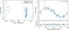 |
Fig. 1 ESPRESSO radial velocity data of L 363-38 used in this analysis. Left: ESPRESSO radial velocities of L 363-38 after subtracting the linear offset and adding the instrumental jitter to the error bars. The measurements obtained during P106 and P108 are shown as open green and filled blue symbols, respectively. Right: phase-folded radial velocity curve of the 8.781d signal. The measurements corresponding to P106 and P108 are defined as in the left panel, while the grey curve shows the best-fit Keplerian model. The bottom panel shows the residuals from the best-fit model. |
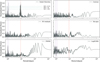 |
Fig. 2 Periodograms of ESPRESSO time series (RV data and stellar activity indicators). The vertical lines mark the position of the companion (P = 8.781 days, red dashed line) and of the aliases (violet dotted lines). A fainter peak at P = 8.781 days is also observed in the contrast indicator (although not significant), but the periodogram of the RV does not show a significant change after applying a linear detrending with any of the indicators. The 0.1%, 1%, and 10% false alarm probability (FAP) levels for the RV periodogram are shown as dashed green horizontal lines. |
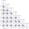 |
Fig. 3 Posterior distribution of the parameters of the Keplerian model for the ESPRESSO data, together with a linear instrumental offset (including the stellar radial velocity) and instrumental jitter. The parameters considered for the Keplerian one-planet model are period (Pb), mean longitude at t = 0 (L0b), radial velocity semi-amplitude (Kb), eccentricity (eb), and argument of periastron (ω). The figure was made using the corner python package (Foreman-Mackey 2016). |
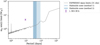 |
Fig. 4 Mass limits computed from the residuals using a bootstrap method (grey line, following Bonfils et al. 2013 and references therein) and position of the companion (purple). The blue shadowed region shows the periods corresponding to the Habitable zone (HZ) computed following two different methods. Method 1 is based on the runaway and maximum Greenhouse limits in Kopparapu et al. (2013, 2014), while method 2 relies on the Bolometric correction of Habets & Heintze (1981) and the scaling values for the inner and outer radius from Kasting et al. (1993), Kasting (1996), and Whitmire & Reynolds (1996). In both cases, the planet reported here orbits at separations much shorter than the HZ. |
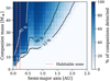 |
Fig. 5 Constraints on companion mass and semi-major axis for planets orbiting around L 363-38, based on the ESPRESSO residuals after subtracting the signal from the planet. The 2D histogram shows the percentage of companions with mass and semi-major axis in a given bin which would be detected with the current ESPRESSO observations, if present. The dashed orange vertical lines indicate the limits of the HZ computed following Kopparapu et al. (2013, 2014, method 1 in Fig. 4; see text for details). |
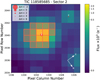 |
Fig. 6 TESS target pixel file (TPF) plot of L 363-38 (TIC 118585685) in Sector 2. The orange area corresponds to the TESS aperture, while the red points indicate the position of Gaia DR2 sources with magnitudes up to Δmag = 6 compared to the target. Our target is well detected, while no additional source is found in the same aperture. The figure has been made using the tfplotter python package (Aller et al. 2020). |
3.4 TESS photometry
The TESS (Ricker et al. 2015) satellite observed L 363-38 in Sectors 2 and 29, obtaining near-continuous 2-min cadence data over ~27 days each. The target pixel file (TPF) for Sector 2 is shown in Fig. 6. The target is well detected, while no additional source with Δm < 6 mag is found in the same extraction aperture. Should the system be oriented edge-on, several transits would have been caught by TESS. Owing to the small host star, for which we assume a radius of 0.274 R⊙ following Pecaut & Mamajek (2013), even an unexpectedly small planetary radius of 1 R⊕ would create a transit depth of 1119 ppm. This would be easily detectable in the TESS data, which show an RMS of 270 ppm when phase-folded on the planetary period and binned into 10-min intervals. The duration of a transit would be expected to be at most 1.8 h.
We therefore searched the TESS data for any transit signals that might stem from L363-38 b. To do so, we used the TESS Science Processing Operations Center (Jenkins et al. 2016) 2-min cadence PDC light curves (Smith et al. 2012; Stumpe et al. 2014), which we additionally detrended by using a boxcar filter with a width of 12 h, much larger than any transits potentially created by L363-38 b. We computed the predicted transit windows during the TESS observations using the radial-velocity data and used the ephemeris obtained – T0 = 59510.457094, P = 8.557 ± 0.012 – to compute the transit windows during the TESS observations5. Visual inspection of the raw and phase-folded data did not reveal any evident transit features at the expected times (see Figs. 7 and 8). To carry out a more robust search for potential low-amplitude transits, we used the transit least-squares (TLS) algorithm (Hippke & Heller 2019). As no significant features were detected, we conclude that L363-38 b is not transiting.
4 Discussion
The analysis described above points to a situation where L 363-38 is orbited by a companion with minimum mass mp sin(i) = 4.67 ± 0.43 M⊕. Assuming the empirical mass-radius relations from Otegi et al. (2020), this minimum mass translates to a minimum radius of rp sin(i) = 1.61 ± 0.06 R⊕ for densities ρ > 3.3 g cm−3, and rp sin(i) = 1.85 ± 0.3 R⊕ for densities ρ < 3.3 g cm−3; using the Forecaster tool (Chen & Kipping 2017), we computed a minimum radius of  . In order to overcome the planetary-mass regime6, the orbital inclination should be i < 0.06°. Assuming a random orientation of the orbital planes, i, this translates to a probability of 99.99% for the companion being a planet. Similarly, the orbital inclination should be i > 15.8° in order for the planet to have a mass smaller than that of Neptune (probability 96%). We caution that the found probabilities may be inaccurate since blind RV surveys are highly efficient at selecting systems that are close to face-on, but in general the information available for this system points to the scenario where the companion lies in the planetary regime. To our knowledge, no additional constraint on the inclination i is currently available.
Figure 4 shows the position of the planet in the mass-period plane together with the mass limits computed from the residuals of the ESPRESSO observations (after subtracting the Keplerian model for one planet) following the method proposed by Bonfils et al. (2013, and references therein). We note that the planet found with this analysis is approximately a factor of five more massive than our detection limits predicted for its period. In addition, it is located at a separation smaller than the inner edge of the HZ. Assuming the stellar properties listed in Table 2, the semi-major axis found with this analysis, and a bond Albedo of 0.3 similar to the values observed for the Earth and Neptune (e.g. Madden & Kaltenegger 2018), we estimate an equilibrium temperature for the planet of Teq ≈ 330 K. According to this analysis, we can exclude the presence of planets with mp sin(i) > 2 − 3 M⊕ in the HZ. Similarly, Fig. 5 suggests that only ~50% of the planets with mp~10 M⊕ would be detected in the HZ, if present, while this percentage goes down to ~15% for mp ~ 5 M⊕.
M dwarfs account for ~75% of the stars in the Milky Way, with an expected occurrence rate of Earth-sized planets (0.5–1.5) R⊕) within the HZ of ~0.25–0.5 planets per star, depending on the study (e.g. Kopparapu 2013; Dressing & Charbonneau 2015). However, the orbital separation of L 363-38 b is at a separation smaller than the inner edge of the HZ, and the planet is unlikely to have liquid water on its surface and to host life. In addition, stellar emission from M dwarfs, for example in the form of flares and winds, could highly affect the planet’s atmosphere and even lead to atmospheric escape (e.g. Segura et al. 2010; Tilley et al. 2019; Kreidberg et al. 2019; Peacock et al. 2020 and references therein), and the accretion of water onto planets around M-stars during formation is extensively discussed in the literature (e.g. Raymond et al. 2007; Lissauer 2007; Hansen 2015; Alibert & Benz 2017). As L 363-38b orbits its star at small separations, it is likely to be tidally locked, which would make habitability even more challenging (e.g. Barnes 2017 and references therein). Observations with new and upcoming telescopes such as the JWST and METIS will be very valuable to characterise the atmosphere of L 363-38 b (or lack thereof) and to investigate these scenarios. However, since the planet is not transiting and cannot be spatially resolved by either of the two instruments, atmospheric studies will only be possible through non-transiting techniques such as phase-curve spectroscopy (e.g. Tinetti et al. 2018; Parmentier & Crossfleld 2018; Glidic et al. 2022).
Figure 9 shows a comparison of the mass, semi-major axis (a), and distance (d) distributions of the confirmed planets in the NASA Exoplanet Archive, and three planets detected with ESPRESSO: L 363-38 b (this work), HD 22469 b (Lillo-Box et al. 2021), and Proxima b (Suárez Mascareño et al. 2020). L 363-38 b and HD 22469 b have very similar parameters, while Proxima b has a lower mass and orbits the nearest stellar neighbour to the Earth. L 363-38 b is found in the lowest 8%, 18%, and 5% of the mp sin(i), a and d distributions of currently confirmed exoplanets, respectively.
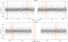 |
Fig. 7 TESS 2-min cadence PDC SAP data of L363-38. The unbinned data are shown as grey points, and the data binned into 30-min intervals are shown in black. The predicted times of transit and their 1-σ probability ranges are indicated with vertical red and orange lines, respectively. |
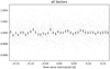 |
Fig. 8 All TESS data phase-folded on the best planetary ephemeris. The unbinned data are shown as grey points, and the data binned into 30-min intervals are shown in black. No indication of a flux drop corresponding to a planetary transit is seen. |
5 Conclusions
We report the discovery of a planet with minimum mass of mp sin(i) = 4.67 ± 0.43 M⊕ orbiting the nearby M dwarf star L 363 38 with a period of P = 8.781 ± 0.007 days, corresponding to a separation of a = 0.048 ± 0.006 AU. We further estimate a minimum radius rp sin(i) ≈ 1.55–2.75 R⊕ and an equilibrium temperature Teq ≈ 330 K. The planet was found during a blind ESPRESSO radial velocity search for planets around nearby stars, as such planets will be prime targets for characterisation with new and upcoming space- and ground-based facilities.
With this study, we further demonstrated the potential of ESPRESSO for investigating planetary systems around nearby M dwarfs. Indeed, the faintness of M stars makes them challenging targets for RV studies using instruments like HARPS behind a 3.6-m telescope, but a spectrograph behind an 8-m telescope such as ESPRESSO can gather sufficient light to precisely measure their RV in an efficient manner. The high precision is crucial to detecting low-mass planets, as well as recognising and modelling signals arising from the stellar activity, which can easily be mistaken for planet signals (e.g. Queloz et al. 2001; Santos et al. 2014; Robertson & Mahadevan 2014; Faria et al. 2020; Suárez Mascareno et al. 2020; Lillo-Box et al. 2021). Moreover, as ESPRESSO extends further into the red part of the spectrum compared to HARPS (λmax~790 nm vs. λmax ~ 690 nm), it is able to detect some of the flux from late M stars which is missed by HARPS.
Based on Kepler and TESS statistics, planets around M dwarfs are expected to occur in multi-planet systems (e.g. Dressing & Charbonneau 2015; Gaidos et al. 2016; Cloutier & Menou 2020; Hadegree-Ullman et al. 2020; Hsu et al. 2020; Feliz et al. 2021). Follow-up observations of L 363-38 with new and upcoming telescopes such as JWST and METIS, as well as astrometric data from Gaia, will be crucial to searching for additional planets further out, as well as characterising the atmosphere of L 363-38 b (or lack thereof) and improving its mass and orbital estimations.
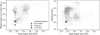 |
Fig. 9 Comparison between the mass, semi-major axis, and distance distributions of the confirmed planets in the NASA Exoplanet Archive (grey shaded dots) and three planets detected with ESPRESSO: HD 22469 b (green circle, Lillo-Box et al. 2021), Proxima b (blue diamond, Suárez Mascareño et al. 2020), and L 363-38 b (purple star, this work). |
Acknowledgements
We thank the referee for helpful comments which improved the clarity of the manuscript. This work has been carried out within the framework of the National Centre of Competence in Research PlanetS supported by the Swiss National Science Foundation. All authors acknowledge the financial support of the SNSF. ML acknowledges support of the Swiss National Science Foundation under grant number PCEFP2_194576. This publication makes use of The Data & Analysis Center for Exoplanets (DACE), which is a facility based at the University of Geneva (CH) dedicated to extrasolar planets data visualisation, exchange and analysis. DACE is a platform of the Swiss National Centre of Competence in Research (NCCR) PlanetS, federating the Swiss expertise in Exoplanet research. The DACE platform is available at https://dace.unige.ch. This work made use of tpfplotter by J. Lillo-Box (publicly available in www.github.com/jlillo/tpfplotter), which also made use of the python packages astropy, lightkurve, matplotlib and numpy. This research has made use of the SIMBAD database, operated at CDS, Strasbourg, France. This research has made use of the NASA Exoplanet Archive, which is operated by the California Institute of Technology, under contract with the National Aeronautics and Space Administration under the Exoplanet Exploration Program. This research made use of Lightkurve, a Python package for Kepler and TESS data analysis (Lightkurve Collaboration 2018). This work has made use of data from the European Space Agency (ESA) mission Gaia (https://www.cosmos.esa.int/gaia), processed by the Gaia Data Processing and Analysis Consortium (DPAC, https://www.cosmos.esa.int/web/gaia/dpac/consortium). Funding for the DPAC has been provided by national institutions, in particular the institutions participating in the Gaia Multilateral Agreement. Authors contributions. LAS carried out the analyses, created part of the figures, and wrote the bulk part of the manuscript. CL reprocessed the ESPRESSO data. CL and JBD supported with the analysis of the RV data. M.L. and A.K. carried out the analysis of the TESS data, and M.L. created part of the figures and wrote part of the manuscript. GC reduced the NaCo data, created the contrast curves, and wrote part of the manuscript. A.B. wrote the initial ESO proposal and some code for the data analysis. S.P.Q. and C.L. initiated the project. All authors discussed the results and commented on the manuscript.
Appendix A Radial velocities
The ESPRESSO radial velocity values used in this analysis are listed in Table A.1
ESPRESSO RV of L 363-38 used in this analysis.
Appendix B Combining RV and HCI constraints
As discussed in the introduction, the goal of oursolarneighbour-hood programme is not only detect new companions, but also to put strong constraints on the possible planetary architecture using the available data and non-detection. In this appendix, we follow the method described in Boehle et al. (2019) and combine the new ESPRESSO RV data with archival NaCo HCI to put constraints on possible additional companions around L 363-38.
Figure B.1 (left) shows the contrast limits obtained from the NaCo HCI observations using the PynPoint pipeline (Stolker et al. 2019). First, the data were corrected for dark current, flat field, and bad pixels (4σ-clipping). The images were aligned using cross-correlation and centred by fitting a 2D Gaussian function to the PSF. Finally, since the field of view was not allowed to rotate during the very short sequence, we applied reference differential imaging (RDI; Lafreniere et al. 2009) based on a principal component analysis (PCA, Amara & Quanz 2012) to remove the central PSF and achieve the highest possible contrast. As a reference star, we chose GL 102, which was observed during the same programme as L 363-38 using the same instrument setup (see Sect. 2.3). The reference star data were calibrated in the same way as those of L 363-38 and were then used to build a principal component library able to model the stellar PSF of our target data. No companion is visible in the residuals, and as is usually done in high-contrast imaging we estimated the contrast limits of our data. These were obtained by inserting artificial companions at different separations (between 0″.05 and 3″.0 in steps of 0″.1) and position angles between 0° and 360° in steps of 60° with different brightness until a signal-to-noise ratio of 5 is reached. A more detailed description of the procedure used to estimate the contrast limits can be found in (Stolker et al. 2019). We further converted them to mass limits assuming a stellar age of 3–8 Gyr and the AMES-Cond evolutionary models (Baraffe et al. 2003), using the functions provided in the species toolkit7 (Stolker et al. 2020). These are shown in Fig. B.1 (right).
Similar to what is presented in Section 3.3, we computed the constraints on the companion mass and semi-major axis for possible additional companions orbiting L 363-38 by following the procedure in Boehle et al. (2019), which combines RV and HCI observations. These calculations are based on the ESPRESSO residuals after subtracting the signal from the planet, as well as on the contrast curves computed for the NaCo images. Specifically, the 2D histogram in the upper part of Fig. B.2 shows the percentage of further companions with mass and semi-major axis in a given bin, which, if present, could be detected with the current ESPRESSO observations (upper left) and NaCo images (upper right) alone. The lower left plot shows the percentage of companions detected when combining both RV and HCI data, while the lower right plot illustrates the fraction of companions that could be detected in the HCI data but not in the RV ones. Figure 5 shows the same as Fig. B.2 (upper left), but on a different scale, which allows a better comparison with the mass limits in Fig. 4.
In order to compute the constraints, we first simulated Keplerian orbits as described in Sect. 3.3, but for a grid with 0 < mp < 100 MJ and 0 < a < 50 AU. For each of orbits we then computed the expected RV signal at the epochs of our ESPRESSO observations, and the projected separation at the epoch of the NaCo observation. If the maximum RV difference measured across the observations (i.e. RVmax - RVmin) is higher than five times the standard deviation of the measured RVs, we considered the planet signal as detectable. On the other hand, a companion is considered as detected in the HCI data if its mass is higher than the mass limit in Fig. B.1 (right) at the predicted separation. The completeness for each combination of mass and semi-major axis was then determined from the percentage of detectable planets in the corresponding bin.
As expected, RV is mostly sensitive to planets with high mass and/or a small semi-major axis, while HCI is more sensitive at larger separations. Because of the short exposure time (160 seconds) and the available band (NB_1.64, λ0 = 1.64μm), the NaCo data do not allow us to constrain low-mass planets, as is the case for the ESPRESSO data, but rather only companions in the brown dwarf and stellar regime. New HCI data, for example from the Spectro-Polarimetric High-contrast Exoplanet REsearch instrument (SPHERE, Beuzit et al. 2019) or from the upcoming Enhanced Resolution Imager and Spectrograph (ERIS, Davies et al. 2018), are therefore crucial to fully exploiting the potential of combining RV and HCl data to better constrain the architecture around nearby stars even in the case of non-detection.
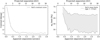 |
Fig. B.1 Limiting contrast curve in NaCo NB_1.64 filter. Right: Limiting companion mass curve computed from the NaCo contrast curve using the AMES-Cond evolutionary models (Baraffe et al. 2003). The shadowed region indicates the spread to due the uncertainty in the stellar age. |
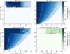 |
Fig. B.2 Constraints on companion mass and semi-major axis for planets orbiting L 363-38, based on the ESPRESSO residuals after subtracting the signal from the planet and on the contrast curve computed for the NaCo observations. The 2D histograms show the percentage of companions with mass and semi-major axis in a given bin that would be detected, if present, with the current ESPRESSO observations (upper left) and NaCo images (upper right). The percentage of companions detected in at least one of the datasets and in the HCl data only are shown in the lower left and lower right panels, respectively. |
References
- Alei, E., Konrad, B. S., Angerhausen, D., et al. 2022, A&A, 665, A106 [NASA ADS] [CrossRef] [EDP Sciences] [Google Scholar]
- Alibert, Y., & Benz, W. 2017, A&A, 598, A5 [NASA ADS] [CrossRef] [EDP Sciences] [Google Scholar]
- Aller, A., Lillo-Box, J., Jones, D., Miranda, L. F., & Barceló Forteza, S. 2020, A&A, 635, A128 [NASA ADS] [CrossRef] [EDP Sciences] [Google Scholar]
- Amara, A., & Quanz, S. P. 2012, MNRAS, 427, 948 [Google Scholar]
- Andrieu, C., & Thoms, J. 2008, Stat. Comput., 18, 343 [Google Scholar]
- Arenou, F., Luri, X., Babusiaux, C., et al. 2018, A&A, 616, A17 [NASA ADS] [CrossRef] [EDP Sciences] [Google Scholar]
- Babusiaux, C., Fabricius, C., Khanna, S., et al. 2023, A&A, in press (https://doi.org/10.1051/0004-6361/202243790) [Google Scholar]
- Baraffe, I., Chabrier, G., Barman, T. S., Allard, F., & Hauschildt, P. H. 2003, A&A, 402, 701 [NASA ADS] [CrossRef] [EDP Sciences] [Google Scholar]
- Barnes, R. 2017, Celest. Mech. Dyn. Astron., 129, 509 [Google Scholar]
- Beuzit, J. L., Vigan, A., Mouillet, D., et al. 2019, A&A, 631, A155 [NASA ADS] [CrossRef] [EDP Sciences] [Google Scholar]
- Boehle, A., Quanz, S. P., Lovis, C., et al. 2019, A&A, 630, A50 [NASA ADS] [CrossRef] [EDP Sciences] [Google Scholar]
- Bonfils, X., Delfosse, X., Udry, S., et al. 2013, A&A, 549, A109 [NASA ADS] [CrossRef] [EDP Sciences] [Google Scholar]
- Boss, A. P., Butler, R. P., Hubbard, W. B., et al. 2007, Trans. Int. Astron. Union Ser. A, 26A, 183 [Google Scholar]
- Brandl, B., Bettonvil, F., van Boekel, R., et al. 2021, The Messenger, 182, 22 [NASA ADS] [Google Scholar]
- Burrows, A., Marley, M., Hubbard, W. B., et al. 1997, ApJ, 491, 856 [Google Scholar]
- Cabral, A., Moitinho, A., Coelho, J., et al. 2010, SPIE Conf. Ser., 7739, 77393W [NASA ADS] [Google Scholar]
- Chen, J., & Kipping, D. 2017, ApJ, 834, 17 [Google Scholar]
- Cloutier, R., & Menou, K. 2020, AJ, 159, 211 [NASA ADS] [CrossRef] [Google Scholar]
- Cumming, A., Butler, R. P., Marcy, G. W., et al. 2008, PASP, 120, 531 [CrossRef] [Google Scholar]
- Cutri, R. M., Skrutskie, M. F., van Dyk, S., et al. 2003, VizieR Online Data Catalog: II/246 [Google Scholar]
- Damasso, M., Sozzetti, A., Lovis, C., et al. 2020, A&A, 642, A31 [NASA ADS] [CrossRef] [EDP Sciences] [Google Scholar]
- Dannert, F. A., Ottiger, M., Quanz, S. P., et al. 2022, A&A, 664, A22 [NASA ADS] [CrossRef] [EDP Sciences] [Google Scholar]
- Davies, R., Esposito, S., Schmid, H. M., et al. 2018, SPIE Conf. Ser., 10702, 1070209 [Google Scholar]
- Delisle, J. B., Ségransan, D., Buchschacher, N., & Alesina, F. 2016, A&A, 590, A134 [NASA ADS] [CrossRef] [EDP Sciences] [Google Scholar]
- Delisle, J. B., Ségransan, D., Dumusque, X., et al. 2018, A&A, 614, A133 [NASA ADS] [CrossRef] [EDP Sciences] [Google Scholar]
- Delisle, J. B., Hara, N., & Ségransan, D. 2020a, A&A, 635, A83 [NASA ADS] [CrossRef] [EDP Sciences] [Google Scholar]
- Delisle, J. B., Hara, N., & Ségransan, D. 2020b, A&A, 638, A95 [EDP Sciences] [Google Scholar]
- Delisle, J. B., Unger, N., Hara, N. C., & Ségransan, D. 2022, A&A, 659, A182 [NASA ADS] [CrossRef] [EDP Sciences] [Google Scholar]
- Díaz, R. F., Almenara, J. M., Santerne, A., et al. 2014, MNRAS, 441, 983 [Google Scholar]
- Díaz, R. F., Ségransan, D., Udry, S., et al. 2016, A&A, 585, A134 [Google Scholar]
- Dressing, C. D., & Charbonneau, D. 2015, ApJ, 807, 45 [Google Scholar]
- Esa 1997, VizieR Online Data Catalog: I/239 [Google Scholar]
- Faria, J. P., Adibekyan, V., Amazo-Gómez, E. M., et al. 2020, A&A, 635, A13 [NASA ADS] [CrossRef] [EDP Sciences] [Google Scholar]
- Faria, J. P., Suárez Mascareño, A., Figueira, P., et al. 2022, A&A, 658, A115 [NASA ADS] [CrossRef] [EDP Sciences] [Google Scholar]
- Feliz, D. L., Plavchan, P., Bianco, S. N., et al. 2021, AJ, 161, 247 [Google Scholar]
- Foreman-Mackey, D. 2016, J. Open Source Softw., 1, 24 [Google Scholar]
- Foreman-Mackey, D., Agol, E., Ambikasaran, S., & Angus, R. 2017, AJ, 154, 220 [Google Scholar]
- Gaia Collaboration (Prusti, T., et al.) 2016, A&A, 595, A1 [NASA ADS] [CrossRef] [EDP Sciences] [Google Scholar]
- Gaia Collaboration (Brown, A. G. A., et al.) 2018, A&A, 616, A1 [NASA ADS] [CrossRef] [EDP Sciences] [Google Scholar]
- Gaia Collaboration (Brown, A. G. A., et al.) 2021, A&A, 649, A1 [NASA ADS] [CrossRef] [EDP Sciences] [Google Scholar]
- Gaidos, E., Mann, A. W., Lépine, S., et al. 2014, MNRAS, 443, 2561 [Google Scholar]
- Gaidos, E., Mann, A. W., Kraus, A. L., & Ireland, M. 2016, MNRAS, 457, 2877 [Google Scholar]
- Gardner, J. P., Mather, J. C., Clampin, M., et al. 2006, Space Sci. Rev., 123, 485 [Google Scholar]
- Gaudi, B. S., Seager, S., Mennesson, B., et al. 2020, ArXiv e-prints [arXiv:2001.06683] [Google Scholar]
- Glidic, K., Schlawin, E., Wiser, L., et al. 2022, AJ, 164, 19 [NASA ADS] [CrossRef] [Google Scholar]
- González Hernández, J. I., Pepe, F., Molaro, P., & Santos, N. C. 2018, in Handbook of Exoplanets, eds. H. J. Deeg, & J. A. Belmonte, 157 [Google Scholar]
- Gordon, T. A., Agol, E., & Foreman-Mackey, D. 2020, AJ, 160, 240 [NASA ADS] [CrossRef] [Google Scholar]
- Haario, H., Saksman, E., & Tamminen, J. 2001, Bernoulli, 7, 223 [CrossRef] [Google Scholar]
- Habets, G. M. H. J., & Heintze, J. R. W. 1981, A&AS, 46, 193 [NASA ADS] [Google Scholar]
- Hadegree-Ullman, K. K., Zink, J. K., Christiansen, J. L., et al. 2020, ApJS, 247, 28 [NASA ADS] [CrossRef] [Google Scholar]
- Hansen, B. M. S. 2015, Int. J. Astrobiol., 14, 267 [NASA ADS] [CrossRef] [Google Scholar]
- Hippke, M., & Heller, R. 2019, A&A, 623, A39 [NASA ADS] [CrossRef] [EDP Sciences] [Google Scholar]
- Hsu, D. C., Ford, E. B., & Terrien, R. 2020, MNRAS, 498, 2249 [Google Scholar]
- Jenkins, J. M., Twicken, J. D., McCauliff, S., et al. 2016, SPIE Conf. Ser., 9913, 99133E [Google Scholar]
- Ji, J.-H., Li, H.-T., Zhang, J.-B., et al. 2022, Res. Astron. Astrophys., 22, 072003 [Google Scholar]
- Jordán, A., Hartman, J. D., Bayliss, D., et al. 2022, AJ, 163, 125 [NASA ADS] [CrossRef] [Google Scholar]
- Kasting, J. F. 1996, in Circumstellar Habitable Zones, ed. L. R. Doyle, 17 [Google Scholar]
- Kasting, J. F., Whitmire, D. P., & Reynolds, R. T. 1993, Icarus, 101, 108 [Google Scholar]
- Konrad, B. S., Alei, E., Quanz, S. P., et al. 2022, A&A, 664, A23 [NASA ADS] [CrossRef] [EDP Sciences] [Google Scholar]
- Kopparapu, R. K. 2013, ApJ, 767, L8 [Google Scholar]
- Kopparapu, R. K., Ramirez, R., Kasting, J. F., et al. 2013, ApJ, 765, 131 [NASA ADS] [CrossRef] [Google Scholar]
- Kopparapu, R. K., Ramirez, R. M., SchottelKotte, J., et al. 2014, ApJ, 787, L29 [Google Scholar]
- Kreidberg, L., Koll, D. D. B., Morley, C., et al. 2019, Nature, 573, 87 [NASA ADS] [CrossRef] [Google Scholar]
- Lafreniere, D., Marois, C., Doyon, R., & Barman, T. 2009, ApJ, 694, L148 [CrossRef] [Google Scholar]
- Leleu, A., Lillo-Box, J., Sestovic, M., et al. 2019, A&A, 624, A46 [NASA ADS] [CrossRef] [EDP Sciences] [Google Scholar]
- Leleu, A., Alibert, Y., Hara, N. C., et al. 2021, A&A, 649, A26 [NASA ADS] [CrossRef] [EDP Sciences] [Google Scholar]
- Lenzen, R., Hartung, M., Brandner, W., et al. 2003, SPIE Conf. Ser., 4841, 944 [Google Scholar]
- Lightkurve Collaboration 2018, Astrophysics Source Code Library [record ascl:1812.013] [Google Scholar]
- Lillo-Box, J., Faria, J. P., Suárez Mascareño, A., et al. 2021, A&A, 654, A60 [NASA ADS] [CrossRef] [EDP Sciences] [Google Scholar]
- Lindegren, L., Hernández, J., Bombrun, A., et al. 2018, A&A, 616, A2 [NASA ADS] [CrossRef] [EDP Sciences] [Google Scholar]
- Lissauer, J. J. 2007, ApJ, 660, L149 [NASA ADS] [CrossRef] [Google Scholar]
- Madden, J. H., & Kaltenegger, L. 2018, Astrobiology, 18, 1559 [NASA ADS] [CrossRef] [Google Scholar]
- Maldonado, J., Micela, G., Baratella, M., et al. 2020, A&A, 644, A68 [EDP Sciences] [Google Scholar]
- Marconi, A., Di Marcantonio, P., D’Odorico, V., et al. 2016, SPIE Conf. Ser., 9908, 990823 [Google Scholar]
- Mayor, M., Pepe, F., Queloz, D., et al. 2003, The Messenger, 114, 20 [NASA ADS] [Google Scholar]
- Mortier, A., Zapatero Osorio, M. R., Malavolta, L., et al. 2020, MNRAS, 499, 5004 [Google Scholar]
- Otegi, J. F., Bouchy, F., & Helled, R. 2020, A&A, 634, A43 [NASA ADS] [CrossRef] [EDP Sciences] [Google Scholar]
- Parmentier, V., & Crossfield, I. J. M. 2018, in Handbook of Exoplanets, eds. H. J. Deeg, & J. A. Belmonte, 116 [Google Scholar]
- Peacock, S., Barman, T., Shkolnik, E. L., et al. 2020, ApJ, 895, 5 [Google Scholar]
- Pecaut, M., & Mamajek, E. E. 2013, in American Astronomical Society Meeting Abstracts, 221, 37.04 [Google Scholar]
- Pepe, F., Mayor, M., Rupprecht, G., et al. 2002, The Messenger, 110, 9 [NASA ADS] [Google Scholar]
- Pepe, F., Cristiani, S., Rebolo, R., et al. 2021, A&A, 645, A96 [NASA ADS] [CrossRef] [EDP Sciences] [Google Scholar]
- Peterson, B. M., Fischer, D., & LUVOIR Science and Technology Definition Team. 2017, in American Astronomical Society Meeting Abstracts, 229, 405.04 [Google Scholar]
- Quanz, S. P., Crossfield, I., Meyer, M. R., Schmalzl, E., & Held, J. 2015, Int. J. Astrobiol., 14, 279 [Google Scholar]
- Quanz, S. P., Kammerer, J., Defrère, D., et al. 2018, SPIE Conf. Ser., 10701, 107011I [NASA ADS] [Google Scholar]
- Quanz, S. P., Ottiger, M., Fontanet, E., et al. 2022, A&A, 664, A21 [NASA ADS] [CrossRef] [EDP Sciences] [Google Scholar]
- Queloz, D., Henry, G. W., Sivan, J. P., et al. 2001, A&A, 379, 279 [NASA ADS] [CrossRef] [EDP Sciences] [Google Scholar]
- Raymond, S. N., Scalo, J., & Meadows, V. S. 2007, ApJ, 669, 606 [Google Scholar]
- Ricker, G. R., Winn, J. N., Vanderspek, R., et al. 2015, J. Astron. Telescopes Instrum. Syst., 1, 014003 [Google Scholar]
- Robertson, P., & Mahadevan, S. 2014, ApJ, 793, L24 [NASA ADS] [CrossRef] [Google Scholar]
- Rousset, G., Lacombe, F., Puget, P., et al. 2003, SPIE Conf. Ser., 4839, 140 [Google Scholar]
- Santos, N. C., Mortier, A., Faria, J. P., et al. 2014, A&A, 566, A35 [NASA ADS] [CrossRef] [EDP Sciences] [Google Scholar]
- Segura, A., Walkowicz, L. M., Meadows, V., Kasting, J., & Hawley, S. 2010, Astrobiology, 10, 751 [Google Scholar]
- Smith, J. C., Stumpe, M. C., Van Cleve, J. E., et al. 2012, PASP, 124, 1000 [Google Scholar]
- Sozzetti, A., Damasso, M., Bonomo, A. S., et al. 2021, A&A, 648, A75 [NASA ADS] [CrossRef] [EDP Sciences] [Google Scholar]
- Spiegel, D. S., Burrows, A., & Milsom, J. A. 2011, ApJ, 727, 57 [Google Scholar]
- Stolker, T., Bonse, M. J., Quanz, S. P., et al. 2019, A&A, 621, A59 [NASA ADS] [CrossRef] [EDP Sciences] [Google Scholar]
- Stolker, T., Quanz, S. P., Todorov, K. O., et al. 2020, A&A, 635, A182 [EDP Sciences] [Google Scholar]
- Stumpe, M. C., Smith, J. C., Catanzarite, J. H., et al. 2014, PASP, 126, 100 [Google Scholar]
- Suárez Mascareño, A., Faria, J. P., Figueira, P., et al. 2020, A&A, 639, A77 [Google Scholar]
- The LUVOIR Team 2019, ArXiv e-prints [arXiv: 1912.06219] [Google Scholar]
- Tilley, M. A., Segura, A., Meadows, V., Hawley, S., & Davenport, J. 2019, Astrobiology, 19, 64 [Google Scholar]
- Tinetti, G., Drossart, P., Eccleston, P., et al. 2018, Exp. Astron., 46, 135 [NASA ADS] [CrossRef] [Google Scholar]
- Toledo-Padrón, B., Lovis, C., Suárez Mascareño, A., et al. 2020, A&A, 641, A92 [Google Scholar]
- Vrijmoet, E. H., Henry, T. J., Jao, W.-C., & Dieterich, S. B. 2020, AJ, 160, 215 [NASA ADS] [CrossRef] [Google Scholar]
- Wenger, M., Ochsenbein, F., Egret, D., et al. 2000, A&AS, 143, 9 [NASA ADS] [CrossRef] [EDP Sciences] [Google Scholar]
- Whitmire, D. P., & Reynolds, R. T. 1996, in Circumstellar Habitable Zones, ed. L. R. Doyle, 117 [Google Scholar]
- Winters, J. G., Charbonneau, D., Henry, T. J., et al. 2021, AJ, 161, 63 [NASA ADS] [CrossRef] [Google Scholar]
- Zechmeister, M., & Kürster, M. 2009, A&A, 496, 577 [CrossRef] [EDP Sciences] [Google Scholar]
The habitable zone (HZ) was computed following two methods. The first one (labelled as method 1 in Fig. 4) is based on the runaway and maximum Greenhouse limits in Kopparapu et al. (2013, 2014), and the second one (method 2) is based on the Bolometric correction of Habets & Heintze (1981) and the scaling values for the inner and outer radius from Kasting et al. (1993), Kasting (1996), and Whitmire & Reynolds (1996).
The period used here slightly differs from the one considered in the rest of the paper, since in order to estimate the mid-transit time T0 we rerun the RV analysis with a different parameterisation of the Keplerian orbits.
Here, we consider the deuterium-burning mass limit M ~13 MJ as a criterion to distinguish between brown dwarfs and planets (e.g. Burrows et al. 1997; Boss et al. 2007; Spiegel et al. 2011).
All Tables
Inferred and derived parameters for the one-planet model of the ESPRESSO radial velocities.
All Figures
|
Fig. 1 ESPRESSO radial velocity data of L 363-38 used in this analysis. Left: ESPRESSO radial velocities of L 363-38 after subtracting the linear offset and adding the instrumental jitter to the error bars. The measurements obtained during P106 and P108 are shown as open green and filled blue symbols, respectively. Right: phase-folded radial velocity curve of the 8.781d signal. The measurements corresponding to P106 and P108 are defined as in the left panel, while the grey curve shows the best-fit Keplerian model. The bottom panel shows the residuals from the best-fit model. |
| In the text | |
|
Fig. 2 Periodograms of ESPRESSO time series (RV data and stellar activity indicators). The vertical lines mark the position of the companion (P = 8.781 days, red dashed line) and of the aliases (violet dotted lines). A fainter peak at P = 8.781 days is also observed in the contrast indicator (although not significant), but the periodogram of the RV does not show a significant change after applying a linear detrending with any of the indicators. The 0.1%, 1%, and 10% false alarm probability (FAP) levels for the RV periodogram are shown as dashed green horizontal lines. |
| In the text | |
|
Fig. 3 Posterior distribution of the parameters of the Keplerian model for the ESPRESSO data, together with a linear instrumental offset (including the stellar radial velocity) and instrumental jitter. The parameters considered for the Keplerian one-planet model are period (Pb), mean longitude at t = 0 (L0b), radial velocity semi-amplitude (Kb), eccentricity (eb), and argument of periastron (ω). The figure was made using the corner python package (Foreman-Mackey 2016). |
| In the text | |
|
Fig. 4 Mass limits computed from the residuals using a bootstrap method (grey line, following Bonfils et al. 2013 and references therein) and position of the companion (purple). The blue shadowed region shows the periods corresponding to the Habitable zone (HZ) computed following two different methods. Method 1 is based on the runaway and maximum Greenhouse limits in Kopparapu et al. (2013, 2014), while method 2 relies on the Bolometric correction of Habets & Heintze (1981) and the scaling values for the inner and outer radius from Kasting et al. (1993), Kasting (1996), and Whitmire & Reynolds (1996). In both cases, the planet reported here orbits at separations much shorter than the HZ. |
| In the text | |
|
Fig. 5 Constraints on companion mass and semi-major axis for planets orbiting around L 363-38, based on the ESPRESSO residuals after subtracting the signal from the planet. The 2D histogram shows the percentage of companions with mass and semi-major axis in a given bin which would be detected with the current ESPRESSO observations, if present. The dashed orange vertical lines indicate the limits of the HZ computed following Kopparapu et al. (2013, 2014, method 1 in Fig. 4; see text for details). |
| In the text | |
|
Fig. 6 TESS target pixel file (TPF) plot of L 363-38 (TIC 118585685) in Sector 2. The orange area corresponds to the TESS aperture, while the red points indicate the position of Gaia DR2 sources with magnitudes up to Δmag = 6 compared to the target. Our target is well detected, while no additional source is found in the same aperture. The figure has been made using the tfplotter python package (Aller et al. 2020). |
| In the text | |
|
Fig. 7 TESS 2-min cadence PDC SAP data of L363-38. The unbinned data are shown as grey points, and the data binned into 30-min intervals are shown in black. The predicted times of transit and their 1-σ probability ranges are indicated with vertical red and orange lines, respectively. |
| In the text | |
|
Fig. 8 All TESS data phase-folded on the best planetary ephemeris. The unbinned data are shown as grey points, and the data binned into 30-min intervals are shown in black. No indication of a flux drop corresponding to a planetary transit is seen. |
| In the text | |
|
Fig. 9 Comparison between the mass, semi-major axis, and distance distributions of the confirmed planets in the NASA Exoplanet Archive (grey shaded dots) and three planets detected with ESPRESSO: HD 22469 b (green circle, Lillo-Box et al. 2021), Proxima b (blue diamond, Suárez Mascareño et al. 2020), and L 363-38 b (purple star, this work). |
| In the text | |
|
Fig. B.1 Limiting contrast curve in NaCo NB_1.64 filter. Right: Limiting companion mass curve computed from the NaCo contrast curve using the AMES-Cond evolutionary models (Baraffe et al. 2003). The shadowed region indicates the spread to due the uncertainty in the stellar age. |
| In the text | |
|
Fig. B.2 Constraints on companion mass and semi-major axis for planets orbiting L 363-38, based on the ESPRESSO residuals after subtracting the signal from the planet and on the contrast curve computed for the NaCo observations. The 2D histograms show the percentage of companions with mass and semi-major axis in a given bin that would be detected, if present, with the current ESPRESSO observations (upper left) and NaCo images (upper right). The percentage of companions detected in at least one of the datasets and in the HCl data only are shown in the lower left and lower right panels, respectively. |
| In the text | |
Current usage metrics show cumulative count of Article Views (full-text article views including HTML views, PDF and ePub downloads, according to the available data) and Abstracts Views on Vision4Press platform.
Data correspond to usage on the plateform after 2015. The current usage metrics is available 48-96 hours after online publication and is updated daily on week days.
Initial download of the metrics may take a while.