© The Authors 2023

1. Introduction

The Λ-cold dark matter (ΛCDM) model is currently considered the standard cosmological framework and provides a satisfactory description of the Universe on the largest scales (Amendola et al. 2018; Planck Collaboration VI 2020). Einstein’s theory of general relativity (GR) is the foundation of all the equations that describe how the Universe evolves and the formation of the cosmic structures we can observe today. During the past few years, GR has been systematically tested both on small and large cosmological scales (see e.g. Beutler et al. 2014; Moresco & Marulli 2017, and references therein), though current measurements are not accurate enough to discriminate among the many alternative theories of gravity that have been proposed to explain the accelerated expansion of the Universe and the growth of cosmic structures.

Clusters of galaxies are the most massive virialised structures in the Universe. Thanks to their high masses and deep gravitational potentials, it is possible to test GR on the scales of these large structures by measuring the gravitational redshift through the peculiar velocity distribution of cluster member galaxies (Cappi 1995; Kim & Croft 2004).

The first detection of the gravitational redshift effect in galaxy clusters was made by Wojtak et al. (2011) using data from the seventh data release (DR7) of the Sloan Digital Sky Survey (SDSS, Abazajian et al. 2009) and the Gaussian Mixture Brightest Cluster Galaxy (GMBCG) sample (Hao et al. 2010). Wojtak et al. (2011) measured the gravitational redshift signal up to 6 Mpc from the cluster centre, which was assumed to be coincident with the brightest cluster galaxy (BCG) position. Their measurements were in agreement with both GR and f(R) theories. Similar analyses have been performed by Jimeno et al. (2015) and Sadeh et al. (2015) using SDSS DR10 data (Ahn et al. 2014). These authors, differently from Wojtak et al. (2011), included in their theoretical model the effects described in Kaiser (2013). In particular, Jimeno et al. (2015) measured the gravitational redshift signal up to 7 Mpc from the cluster centre, analysing three different cluster catalogues: the GMBCG, the sample described in Wen et al. (2012, WHL12), and the RedMaPPer cluster sample (Rykoff et al. 2014). The gravitational redshift effect was measured both as a function of the distance from the cluster centre and as a function of the cluster masses. Jimeno et al. (2015) detected a significant signal in the GMBCG and RedMaPPer samples, while the measurements in the WHL12 sample were not in agreement with theoretical expectations. The latest attempt was carried out by Mpetha et al. (2021), who analysed the SPectroscopic IDentification of ERosita Sources (SPIDERS, Clerc et al. 2020) survey. In particular, they considered three different definitions of the cluster centre: the BCG position, the redMaPPer identified central galaxies, and the peak of the X-ray emission. With all the three centre definitions, they obtained a clear detection of the gravitational redshift, but their results could not discriminate between GR and f(R) predictions.

Our work aims to update and improve these past analyses by exploiting the new galaxy data released by the SDSS DR16 (Ahumada et al. 2020) and the new galaxy cluster sample provided by Wen & Han (2015, WH15). We refined the measurement method and the theoretical model to improve the accuracy of the analysis. Thanks to these improvements, we were able to reduce the measurement errors by about 30% with respect to the works of Sadeh et al. (2015) and Mpetha et al. (2021), up to a distance of almost 3 Mpc from the cluster centres. The huge number of measured redshifts inside our sample allowed us to perform an accurate Bayesian analysis, imposing new constraints on GR on megaparsec scales.

The paper is organised as follows. In Sect. 2 we introduce the analysed cluster catalogue and the SDSS DR16 galaxy sample, while in Sect. 3 we describe the new cluster member catalogue that we constructed for this analysis. In Sect. 4 we present the theoretical predictions on the galaxy line-of-sight velocity distribution offsets as a function of the distance from the cluster centre in three different gravity theories. The method used to measure this statistic from the observed galaxy redshifts is described in Sect. 7. In Sect. 8 we present the main results of our work. In Sect. 9 we conclude with closing remarks and future prospects. Finally, in Appendix A we describe the analysis of the systematic uncertainties affecting our measurements.

In this work all the cosmological calculations were performed assuming a flat ΛCDM model, with Ω_m = 0.3153 and H₀ = 67.36 km s⁻¹ Mpc⁻¹ (Planck Collaboration VI 2020, Paper VI: Table 2, TT,TE,EE+lowE+lensing,). The whole cosmological analysis was performed with the CosmoBolognaLib (CBL, Marulli et al. 2016), a large set of ‘free software’ C++/Python libraries that provides an efficient numerical environment for statistical investigations of the large-scale structure of the Universe. The new likelihood functions for fitting the velocity distributions and computing GR and the alternative gravity theory predictions, will be released in the forthcoming public version of the CBL.

2. Data

2.1. The cluster sample

In this work we exploit the galaxy cluster sample described in Wen & Han (2015), which is an updated version of the WHL12 cluster catalogue. The WHL12 sample was built using the SDSS-III photometric data (SDSS DR8, Aihara et al. 2011). The method used to identify the galaxy clusters was based on a ‘friend-of-friend’ algorithm. In practice, a cluster was identified if more than eight member galaxies, with an r-band absolute magnitude smaller than −21, were found within a radius of 0.5 Mpc and within a photometric redshift range of 0.04(1 + z). After that, the BCG was recognised among the cluster members and it was taken as the cluster centre. WHL12 calculated the total luminosity within a radius of 1 Mpc, L_1 Mpc, then by using a scaling relation between L_1 Mpc and the cluster virial radius r₂₀₀, they computed r₂₀₀. The total luminosity within the r₂₀₀ radius and the cluster richness were eventually computed. The optical richness, R_L200, was used as a proxy for the cluster mass, M₂₀₀, within r₂₀₀.

In the WH15 catalogue, the cluster masses have been recalibrated. Specifically, WH15 exploited new cluster mass estimations from X-ray and Sunyaev–Zeldovich effect measurements to recalibrate the richness-mass relation within the redshift range 0.05 < z < 0.75. The calibrated relation can be expressed as follows:

$$\begin{array}{c}\hfill log(M_{500})=14+(1.08\pm 0.02)log(R_{\text{L}500})-(1.37\pm 0.02),\end{array}$$(1)

where M₅₀₀ and R_L500 are the mass and the optical richness within r₅₀₀¹, respectively. By using the spectroscopic data of the SDSS DR12 (Alam et al. 2015), the authors also extended the number of clusters with spectroscopic redshifts.

The final sample includes the data of BCG angular positions and redshifts of 132 684 clusters within the redshift range 0.05 ≤ z ≤ 0.8. The identified clusters have an average redshift of ⟨z⟩ = 0.37, an average mass of ⟨M₅₀₀⟩ = 1.4 × 10¹⁴ M_⊙, and an average radius of ⟨r₅₀₀⟩ = 0.67 Mpc. The authors claimed that this sample is almost complete in the redshift range 0.05 ≤ z < 0.42 and for masses above 10¹⁴ M_⊙.

2.2. The spectroscopic galaxy samples

We exploited the galaxy coordinates and spectroscopic redshifts derived from SDSS DR16 (Ahumada et al. 2020). Specifically, we analysed the data collected by the Baryon Oscillation Spectroscopic Survey (BOSS, Dawson et al. 2013), the Extended Baryon Oscillation Spectroscopic Survey (eBOSS, Dawson et al. 2016), and the Legacy Survey obtained as part of the SDSS-I and SDSS-II programmes (York et al. 2000). Although the spectroscopic data and the sky coverage of the galaxy samples have remained unchanged during the past years, the imaging and the spectroscopic pipelines have been improved in subsequent SDSS data releases. Therefore, in this work we used the data of the latest release.

The Legacy Survey covers a total sky area of 8032 deg² and it is composed of two galaxy samples: the ‘Main sample’, a magnitude-limited sample of galaxies with a mean redshift of z ≃ 0.1 (Strauss et al. 2002) and the ‘luminous red galaxies’ (LRGs) sample, a volume-limited sample up to z ≃ 0.4 (Eisenstein et al. 2001).

Within the Legacy Survey, we selected the galaxies with the most reliable spectra and the lowest redshift errors. Specifically, we selected the objects in the catalogue that had the following flags²: SPECPRIMARY equal to 1, CLASS ‘Galaxy’, ZWARNING equal to 0, 4, or 16, ZERR less than 6 × 10⁻⁴, and Z between 0.05 and 0.75 included. These selections were applied to avoid multiple entries of the same object in the final catalogue, and to include only those galaxies with reliable spectroscopic redshift measurements. Moreover, we selected the redshift range where the richness-mass relation of the cluster sample had been calibrated. We found almost 760 000 galaxies within the Legacy Survey that were useful for our analysis.

BOSS is part of the six-year SDSS-III programme, which obtained the spectroscopic redshifts of about 1.5 million LRGs out to a redshift of almost 0.7. We also included data from the eBOSS, which collected the spectroscopic redshifts of LRGs, emitting luminous red galaxies (eLRGs), and quasars (QSO), up to z = 3.5. We selected galaxies from these surveys using similar flags³ to the Legacy Survey case. We considered objects that had the flag SPECPRIMARY equal to 1 and we selected those that had CLASS_NOQSO equal to ‘Galaxy’. We considered the galaxies with the most reliable redshift estimations by selecting those that had the flag ZWARNING_NOQSO equal to 0, 4, or 16, and the flag ZERR_NOQSO less than 6 × 10⁻⁴. Finally, we selected the galaxies with redshift between 0.05 and 0.75 by using the flag Z_NOQSO. These selections were applied for the same reasons explained previously for the Legacy Survey. We found about 1.9 million galaxies useful for our analysis within BOSS and eBOSS.

Table 1 shows the selections we made on the galaxy sample.

Figure 1 shows the redshift distribution of the galaxies inside the exploited sample. The mean galaxy redshift within the Legacy Survey is z ≃ 0.16, while BOSS and eBOSS galaxies have a mean redshift of z ≃ 0.48.

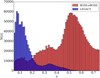Fig. 1. Redshift distribution of the selected galaxies. The blue histogram represents the galaxy redshift distribution of the Legacy Survey, while the red histogram shows the distribution of BOSS and eBOSS.

3. Searching for cluster member galaxies

To recover the signal of the gravitational redshift effect, it is necessary to calculate the distribution of the galaxy line-of-sight velocity offsets, Δ (see Sect. 4), as a function of the distance from the cluster centre. We constructed a new catalogue of cluster member galaxies by cross-correlating the WH15 cluster catalogue, described in Sect. 2.1, with the public spectroscopic galaxy data, described in Sect. 2.2. Then we computed the projected transverse distance, r_⊥, and the Δ of all the galaxies with respect to each cluster centre. We define the latter as the mean value of the angular positions and redshifts of the closest galaxies to the BCG, considering objects having a transverse distance smaller than r₅₀₀ from the BCG. Below we explain in details how we selected our data set.

The WH15 sample provided the BCG angular positions of the identified clusters. However, most of the BCGs did not have a spectroscopic redshift measurement. Thus, to increase the number of the available spectroscopic BCGs, we cross-matched the cluster samples with the considered galaxy catalogue. We took into account the fact that, according to the SDSS specifications, two galaxies are considered the same object if they are closer than 3 arcsec in the Legacy Survey case, and 2 arcsec in the BOSS and eBOSS cases. Thus, we considered the cluster member galaxies only inside clusters that had the BCG identified in the galaxy sample described in Sect. 2.2. The advantage of doing so is that we increased the statistics of the cluster samples, and we made sure that we only analysed clusters that had reliable spectroscopic redshift measurements for their BCGs. From the cross-matching of the WH15 catalogue and the SDSS data, we obtained 85 588 clusters with a spectroscopic BCG identification; 47 779 of these had the BCG identified in BOSS and eBOSS, while the other 37 809 clusters had the BCG identified in the Legacy Survey.

Once we had identified the cluster BCGs, we searched for the closest galaxies to define a new cluster centre. To do this, we computed the projected transverse distances, r_⊥, and the line-of-sight velocities of all the SDSS galaxies with respect to the BCGs. We kept the galaxies that lay within r_⊥ < r₅₀₀ and |Δ|< 2500 km s⁻¹ from the BCGs. For each cluster in our sample, we computed the average value of the redshifts and angular positions of the selected galaxies, including the BCG, and we defined these averages as the new cluster centres. It should be noted that this centre definition has never been used in past literature works to measure the gravitational redshift in galaxy clusters. Instead, it was always assumed that the cluster centre coincides exactly with the BCG position (Wojtak et al. 2011; Sadeh et al. 2015; Jimeno et al. 2015). We find instead that the average of the member galaxy positions provides a more reliable location of the centre than the BCG, because the BCG could be misidentified due to the surface brightness modulation effect. In fact, peculiar velocities can change the ranking of the two cluster brightest galaxies. In order to investigate the impact of assuming the average galaxy positions as the centre of the cluster potential wells, we compared our results to the results obtained by instead assuming the BCG as the cluster centre. We find that the measurements are in substantial disagreement with the theoretical predictions in the BCG centre case, showing positive values of the mean of the galaxy velocity distribution for r_⊥ < 2r₅₀₀. Similar results were obtained by Jimeno et al. (2015) when analysing the WHL12 cluster sample. The detailed description of the analysis we carried out assuming the BCG as the cluster centre is presented in Appendix A.1.

Once we had defined the cluster centre, we re-selected the cluster member galaxies. We considered a galaxy to be a cluster member if it lay within a separation of r_⊥ < 4 r₅₀₀ and |Δ|< 4000 km s⁻¹ from the cluster centre. We adopted a lower limit in the transverse distance, which was about half the size considered in past literature works, in order not to depart too much from the cluster virialised region. On the other hand, this was the same selection threshold on the galaxy line-of-sight velocity adopted in Wojtak et al. (2011) and Sadeh et al. (2015). Hence, we created a cluster member catalogue, given the galaxy position average described above as the centre, and we retrieved the galaxy line-of-sight velocity distribution⁴. It should be noted that the galaxies that had |Δ| between 3000 km s⁻¹ and 4000 km s⁻¹ were considered as either foreground or background galaxies, which were not gravitationally bound to any cluster. Nevertheless, we also included these galaxies to correct the velocity distribution of the galaxies that effectively lay within the cluster gravitational potential well, as described in Sect. 7.1.

Before proceeding with the measurement of the gravitational redshift, we made some further selections on the cluster member catalogue. Firstly, we discarded the clusters that had a redshift above 0.5. We made this selection in order to avoid the redshift range where the probability of a false cluster identification was higher than about 5%, as estimated in WHL12 and WH15. Moreover, with this selection we restricted the analysis to a redshift range where the impact of possibly incorrect cosmological model parameters was less significant (see e.g. Wojtak et al. 2011). Then, we considered only the clusters that had at least four associated galaxies, and where the average centre was computed using data of at least three galaxies, including the BCG. We considered this selection in order to be conservative, considering only the clusters that had their centres estimated with a sufficient number of galaxies. When the cluster mass increases, the gravitational redshift effect becomes stronger and the probability of having a cluster false identification decreases. Moreover, the galaxy line-of-sight velocity offsets measured in low-mass clusters are more affected by the galaxy peculiar velocities than in high-mass clusters (Kim & Croft 2004). To minimise these possible sources of systematic uncertainties, we selected the clusters that had a mass above 1.5 × 10¹⁴ M_⊙. The effects of all these selections are discussed in Appendix A.2. Finally, we discarded the configurations in which Legacy Survey and BOSS-eBOSS spectra were mixed together, that is to say, the cluster member galaxies (comprising the BCGs) of the Legacy cluster sample were selected only from the Legacy spectroscopic galaxy sample, while those of the BOSS-eBOSS cluster sample were selected only from the BOSS-eBOSS galaxy sample. We made this choice because the mixed configurations tend to suppress the gravitational redshift signal for small values of transverse distances, as demonstrated by Sadeh et al. (2015). It should be noted that all these conservative selections were possible thanks to the high statistics of the galaxy and cluster samples we analysed.

Table 2 shows the selections we made on the cluster sample.

The final selected sample consisted of 3058 galaxy clusters and 49 243 associated member galaxies. The average redshift is ⟨z⟩ = 0.25 and the average mass was ⟨M₅₀₀⟩ = 2.75 × 10¹⁴ M_⊙. The number of galaxy clusters in our sample was similar to the one of Jimeno et al. (2015). However, we selected the cluster member galaxies using an upper transverse distance limit, which was half the size of the one used in that work. Moreover, to minimise the problems created by the false cluster identification, we applied more conservative selections. The average redshift of our sample was similar to the redshifts of the samples analysed by Wojtak et al. (2011) and Jimeno et al. (2015), while we selected clusters with higher masses on average.

Figure 2 shows the redshift and mass distributions of the WH15 clusters within the redshift and mass ranges where the richness-mass relation was calibrated, that is 0.05 < z < 0.75 and 3 × 10¹³ M_⊙. The figure also shows the resulting distributions after each selection was applied individually, and the final selected sample analysed in this work.

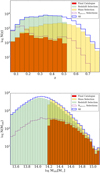Fig. 2. Redshift (top panel) and mass distribution (bottom panel) of the selected cluster sample. The solid blue histograms represent the distributions of all WL15 clusters within the redshift and mass ranges where the richness-mass relation was calibrated. The yellow histograms show the distributions of the clusters with mass above 1.5 × 1014 M⊙, while the green histograms show the distributions of the clusters with z < 0.5. The dashed purple histograms show the distributions of the clusters that have at least four associated galaxies. Finally, the red histograms represent the distributions of the final selected cluster sample.

Figure 3 shows the angular maps around four galaxy clusters of the final selected sample analysed in this work. Both member and field galaxies are shown, along with their line-of-sight velocities. The objects are representative examples of four different cluster types: a low-redshift massive cluster with a large number of identified galaxy members; a high-redshift small cluster though with a sufficient number of members; an isolated cluster with only a few identified members; and two small close clusters. It should be noted that the BCG positions are not always near to the cluster centres identified by the galaxy member positions.

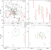Fig. 3. Angular maps around four galaxy clusters of the selected sample. The black points represent the cluster member galaxies, while the red squares show the positions of the field galaxies. The gold diamond shows the cluster centres and the cyan star represents the cluster BCGs. The dashed green circle indicates the cluster r500 radii. The arrows show the galaxy line-of-sight velocities with respect to the cluster centres. The arrows pointing upwards (downwards) represent positive (negative) velocities. The objects are representative examples of four different cluster types: a low-redshift massive cluster with a large number of identified galaxy members (top left panel); a high-redshift small cluster, though with a sufficient number of members (top right panel); an isolated cluster with only a few identified members (bottom left panel); and two small close clusters (bottom right panel).

4. Predicting gravitational redshift in different gravity theories

Gravity theories, overall, predict that photon frequencies are redshifted by a gravitational field. When a photon with wavelength λ is emitted inside a gravitational potential ϕ, it loses energy when it climbs up in the gravitational potential well, and is consequently redshifted. The gravitational redshift, z_g, observed at infinity in the weak field limit, can be expressed as follows:

$$\begin{array}{c}\hfill z_g:=\frac{\mathrm{\Delta }\lambda }{\lambda }\simeq \frac{\mathrm{\Delta }\varphi }{c^2},\end{array}$$(2)

where Δλ and Δϕ are, respectively, the wavelength and the potential differences between the positions where the photon is emitted and where it is observed.

If we consider a galaxy, which resides inside a cluster, as a source of photons, the measurement of the total observed galaxy redshift, z_obs, is the sum of different effects, where the main components are the following: the cosmological redshift, z_cosm, the peculiar redshift, caused by the motion of the galaxy within the cluster, z_pec, and the gravitational redshift, z_g:

$$\begin{array}{c}\hfill ln(1+z_{\mathrm{obs}})=ln(1+z_{\mathrm{cosm}})+ln(1+z_{\mathrm{pec}})+ln(1+z_{\mathrm{g}}).\end{array}$$(3)

We used differences in the logarithm of the redshifts, as previously done by Mpetha et al. (2021). Baldry (2018) demonstrated that this provides a better approximation of the galaxy line-of-sight velocity, with respect to assuming z = v/c. The gravitational redshift depends on the cluster gravitational potential, and thus on the mass distribution around the galaxy. For a typical cluster mass of 10¹⁴ M_⊙, the gravitational redshift is estimated to be cz_g ≃ 10 km s⁻¹ (Cappi 1995; Kim & Croft 2004), which is about two orders of magnitude smaller than the peculiar redshift. The tiny effect of the gravitational redshift can be detected only when the number of analysed galaxies is large enough, that is N_gal ≳ 10⁴ (Zhao et al. 2013). Therefore, stacked data of large samples of clusters and cluster member galaxies are necessary to measure the gravitational redshift effect with reasonable accuracy.

To disentangle the gravitational redshift from the other components, we measured the distribution of the galaxy line-of-sight velocities in the cluster reference frame (Kim & Croft 2004). The line-of-sight velocity offset is defined as follows (Mpetha et al. 2021):

$$\begin{array}{c}\hfill \mathrm{\Delta }:=c[ln(1+z_{\mathrm{obs}})-ln(1+z_{\mathrm{cen}})],\end{array}$$(4)

where z_cen is the redshift of the cluster centre. By construction, the line-of-sight velocity offset does not depend on the cosmological redshift component, which is the same in the two terms of Eq. (4), and thus it cancels out. The Δ distribution of all the galaxy cluster members can be modelled as a quasi-Gaussian function with a non-zero mean velocity, $\overline{\mathrm{\Delta }}$. The value of $\overline{\mathrm{\Delta }}$ depends on the spatial variation of the gravitational potential. This effect is present also in the most popular alternative theories of gravity, which aim to modify GR, possibly explaining the Universe accelerated expansion without a dark energy component. Thus, the value of the Δ distribution mean is the quantity of interest in this study. Specifically, we focus on the dependence of $\overline{\mathrm{\Delta }}$ on the distance from the cluster centre.

4.1. General relativity

The distribution of line-of-sight velocity offsets between cluster member galaxies and their host cluster centre, defined in Eq. (4), is expected to have an average value that is blueshifted (Cappi 1995; Kim & Croft 2004). In fact, photons experience the largest gravitational redshifting at the minimum of the cluster potential wells, and the gravitational redshift effect decreases towards the cluster outskirts, as the gravitational potential well decreases as well. Therefore, comparing the redshift of the cluster centre with the redshifts of member galaxies gives the net result of a blueshift. For a single galaxy, the gravitational redshift, expressed as a velocity offset, is given by:

$$\begin{array}{c}\hfill \mathrm{\Delta }=\frac{\varphi (0)-\varphi (r)}{c},\end{array}$$(5)

where r is the distance from the cluster centre. Generally, only the projected distance from the cluster centre, r_⊥, is known with sufficient accuracy. Thus, to compute the gravitational redshift signal, the density along the line of sight to that distance has to be integrated along with the potential difference.

In this work we assumed that the cluster density profile follows the Navarro-Frank-White radial profile (NFW, Navarro et al. 1995). Moreover, we used the projected distance from the centre of the cluster in units of r₅₀₀, because scaling the separation between galaxies and the associated cluster centres takes advantage of the cluster self-similarity. Moreover, stacking data by considering comoving distances is not ideal, as clusters can have a large range of sizes, and therefore different masses and densities at the same distance from the centre. The NFW density profile of a cluster, in units of its radius r₅₀₀, can be expressed as follows (Łokas & Mamon 2001):

$$\begin{array}{c}\hfill \rho (\stackrel{\sim }{r})=\frac{M_{500}{c}_{500}^{2}g(c_{500})}{4\pi r_{500}^3\stackrel{\sim }{r}{(1+c_{500}\stackrel{\sim }{r})}^2},\end{array}$$(6)

where $\stackrel{\sim }{r}:=r/r_{500}$, c₅₀₀ is the cluster concentration parameter defined as c₅₀₀ := r₅₀₀/r_s, r_s is the so-called scale radius of the cluster, and the function g(c₅₀₀) can be expressed as follows:

$$\begin{array}{c}\hfill g(c_{500})={[ln(1+c_{500})-\frac{c_{500}}{1+c_{500}}]}^{-1}.\end{array}$$(7)

The gravitational potential, associated with the density distribution given by Eq. (6), results in:

$$\begin{array}{c}\hfill \varphi (\stackrel{\sim }{r})=-g(c_{500})\frac{G{M}_{500}}{r_{500}}\frac{ln(1+c_{500}\stackrel{\sim }{r})}{\stackrel{\sim }{r}}.\end{array}$$(8)

Hence, under these assumptions, the gravitational redshift for a single cluster (i.e. the mean of the cluster member galaxies velocity distribution) can be written as follows:

$$\begin{array}{c}\hfill {\overline{\mathrm{\Delta }}}_{c,gz}({\stackrel{\sim }{r}}_{\perp })=\frac{2r_{500}}{c\mathrm{\Sigma }({\stackrel{\sim }{r}}_{\perp })}{\displaystyle {\int }_{{\stackrel{\sim }{r}}_{\perp }}^{\infty }}[\varphi (0)-\varphi (\stackrel{\sim }{r})]\frac{\rho (\stackrel{\sim }{r})\stackrel{\sim }{r}\text{d}\stackrel{\sim }{r}}{\sqrt{{\stackrel{\sim }{r}}^2-{\stackrel{\sim }{r}}_{\perp }^2}},\end{array}$$(9)

where ${\stackrel{\sim }{r}}_{\perp }$ is the projected distance from the centre of the cluster in units of r₅₀₀. $\mathrm{\Sigma }({\stackrel{\sim }{r}}_{\perp })$ is the surface mass density profile computed from the integration of the NFW density profile along the line of sight:

$$\begin{array}{c}\hfill \mathrm{\Sigma }({\stackrel{\sim }{r}}_{\perp })=2r_{500}{\displaystyle {\int }_{{\stackrel{\sim }{r}}_{\perp }}^{\infty }}\frac{\rho (\stackrel{\sim }{r})\stackrel{\sim }{r}}{\sqrt{{\stackrel{\sim }{r}}^2-{\stackrel{\sim }{r}}_{\perp }^2}}\text{d}\stackrel{\sim }{r}.\end{array}$$(10)

Here we are assuming that a stacked sample of many clusters exhibits spherical symmetry, even though it is not often the case for a single cluster (Kim & Croft 2004). Following Wojtak et al. (2011), the gravitational redshift signal for a stacked cluster sample can be calculated by convolving the gravitational redshift profile for a single cluster with the cluster mass distribution. This operation can be expressed as follows:

$$\begin{array}{c}\hfill {\overline{\mathrm{\Delta }}}_{\mathit{gz}}({\stackrel{\sim }{r}}_{\perp })=\frac{{\int }_{M_{\min }}^{M_{\max }}{\mathrm{\Delta }}_{c,gz}({\stackrel{\sim }{r}}_{\perp })\mathrm{\Sigma }({\stackrel{\sim }{r}}_{\perp })(\text{d}N/\text{d}{M}_{500})\text{d}{M}_{500}}{{\int }_{M_{\min }}^{M_{\max }}\mathrm{\Sigma }({\stackrel{\sim }{r}}_{\perp })(\text{d}N/\text{d}{M}_{500})\text{d}{M}_{500}}.\end{array}$$(11)

Equation (11) can be used to compute the gravitational redshift effect for a stacked cluster sample as a function of the projected radius.

Equation (11) is valid in any theory of gravity, although different theories predict different gravitational accelerations experienced by photons within the clusters. In particular, in alternative gravity theories, the Newtonian constant G is usually replaced by a function of the cluster radius.

In the following sections, we describe the gravitational acceleration as a function of the cluster radius, g(r), predicted by two different gravity theories: the f(R) model (see Sotiriou & Faraoni 2010, for a complete review) and the Dvali–Gabadadze–Porrati model (DGP, Dvali et al. 2000). These two alternative gravity theories appreciably modify the gravity interaction on the largest scales to reproduce the Universe accelerated expansion, but restore GR locally, satisfying all current constraints if their parameters are properly adjusted.

4.2. The f(R) gravity model

In GR, the Einstein-Hilbert action, S, which is the integral of the Lagrangian density over the space-time coordinates, describes the interaction between matter and gravity and can be expressed as follows:

$$\begin{array}{c}\hfill S={\displaystyle \int }{\mathrm{d}}^{4}x\sqrt{-g}[\frac{M_{\mathit{pl}}^2}{2}(R-2\mathrm{\Lambda })+L_m],\end{array}$$(12)

where $M_{\mathit{pl}}=\sqrt{1/8\pi G}$ is the reduced Planck mass, R is the Ricci scalar, L_m is the matter Lagrangian, and g is the Friedmann–Lemaître–Robertson–Walker metric determinant.

Starobinsky (1980) demonstrates that it is possible to modify Eq. (12) to describe a consistent gravity theory as follows:

$$\begin{array}{c}\hfill S={\displaystyle \int }{\mathrm{d}}^{4}x\sqrt{-g}[\frac{M_{\mathit{pl}}^2}{2}(R-f(R))+L_m],\end{array}$$(13)

where the cosmological constant is replaced by a function of the Ricci scalar, f(R), which is an unknown function. f(R) models are scalar-tensor theories, where the scalar degree of freedom is given by f_R ≡ df/dR, which mediates the relation between density and space-time curvature. The theory is stable under perturbations if f_R < 0. The Starobinsky (1980) model is constructed to reproduce the properties of the ΛCDM framework on linear scales. Moreover, GR is restored on the smallest scales, thus fulfilling local constraints.

Schmidt (2010) showed that in the strong field scenario, |f_R0| = 10⁻⁴, the f(R) theory predicts a 4/3 enhancement of the gravitational force for all halo masses, that is G_f(R) = 4/3G. Thus, the gravitational potential, given by Eq. (8), is significantly enhanced, and the gravitational redshift effect, given by Eq. (9), is consequently stronger than in GR. Following Wojtak et al. (2011) and Mpetha et al. (2021), in this work we considered the f(R) theory in this strong field scenario. Although the strong field scenario has been already excluded by different observations (e.g. Terukina et al. 2014; Wilcox et al. 2015), we considered this model as comparison because its predictions are significantly enough different from GR to be detectable with current gravitational redshift measurements.

4.3. The Dvali–Gabadadze–Porrati gravity model

In the DGP braneworld scenario (Dvali et al. 2000), matter and radiation live on a four-dimensional brane embedded in a five-dimensional Minkowski space. The action is constructed so that on scales larger than the so-called crossover scale, r_c, gravity is five-dimensional, while it becomes four-dimensional on scales smaller than r_c. Thus, the gravitational potential is 1/r at short distances for the sources localised on the brane. As a result, an observer on the brane will experience Newtonian gravity, despite the fact that gravity propagates in extra space, which is flat and has an infinite size. This model admits a homogeneous cosmological solution on the brane, which obeys a modified Friedmann equation (Deffayet 2001):

$$\begin{array}{c}\hfill H^2\pm \frac{H}{r_c}=8\pi G(\overline{\rho }+{\rho }_{\mathrm{DE}}),\end{array}$$(14)

where ρ_DE is the density associated with the cosmological constant. The sign on the left-hand side of Eq. (14) is determined by the choice of the embedding of the brane. The negative sign is the so-called self-accelerating branch, which allows for accelerated Universe expansion even in the absence of a cosmological constant. The positive sign is the so-called normal branch, which does not exhibit self-acceleration. On scales smaller than r_c, the DGP models can be described as a scalar-tensor theory where the brane-bending mode φ mediates an additional attractive (normal branch) or repulsive (self-accelerating branch) force (Nicolis & Rattazzi 2004).

In DGP models the gravitational forces are governed by the equation:

$$\begin{array}{c}\hfill \mathrm{\nabla }\varphi =\mathrm{\nabla }{\varphi }_N+\frac{1}{2}\mathrm{\nabla }\phi ,\end{array}$$(15)

where ∇ϕ_N is the Newtonian gravitational potential. It is possible to find an analytical solution for φ in the case of a spherically symmetric mass. In particular, it is possible to obtain an equation for the φ gradient, which can be expressed as follows:

$$\begin{array}{c}\hfill \frac{\mathrm{d}\phi }{\mathrm{d}r}=\frac{G\delta M(<r)}{r^2}\frac{4}{3\beta }g\left(\frac{r}{r_{\ast }(r)}\right),\end{array}$$(16)

where the function g(y) is:

$$\begin{array}{c}\hfill g\left(y\right)=y^3[\sqrt{1+y^{-3}}-1],\end{array}$$(17)

and r_*(r) is the so-called r-dependent Vainsthein radius. The function r/r_* depends on the average over-density δρ(< r), within r. It is possible to re-scale this function to a halo with mass M_Δ and radius R_Δ, determined by a fixed over-density Δ. Thus, we obtain:

$$\begin{array}{c}\hfill \frac{r}{r_{\ast }(r)}={(\epsilon \mathrm{\Delta })}^{-1/3}x{\left[\frac{M(<x)}{M_{\mathrm{\Delta }}}\right]}^{-1/3},\end{array}$$(18)

where x := r/R_Δ and the quantity ε is determined by the background cosmology. By combining these equations, Schmidt (2010) calculated the g_DGP(r) parameter, which quantifies the differences between GR and DGP models:

$$\begin{array}{c}\hfill g_{\mathrm{DGP}}(r)=1+\frac{2}{3\beta }g\left(\frac{r}{r_{\ast }(r)}\right).\end{array}$$(19)

On the largest scales $g\left(\frac{r}{r_{\ast }(r)}\right)$ tends to 1/2, so we obtain g_DGP = g_DGP, lin = 1 + 1/(3β). On the other hand, on the smallest scales where r ≪ r_*, the modified forces are suppressed.

In this work, we considered a self-accelerating model (sDPG model) with ρ_DE = 0, and r_c = 6000 Mpc, which was adjusted to best match the constraints derived from cosmic microwave background observations and Universe expansion history (Fang et al. 2008). We made this choice to test a model that does not need a dark energy component to explain the Universe accelerated expansion. Marulli et al. (2021) found that the redshift-space clustering anisotropies of the two-point correlation function of the same cluster sample exploited in this work are in good agreement with the predictions of this DGP model.

Schmidt (2010) showed that this model predicts a reduction of the gravitational force, independently of the halo masses. In this work we set β = −1.15 in Eq. (19), and ε = 0.32 in Eq. (18) at z = 0, in order to reproduce the Schmidt (2010) simulation results. The model predictions were significantly affected by the values of the two parameters. In fact, with β = 1/3 we recovered GR on the largest scales.

5. Other relativistic and observational effects

There are other effects beyond the gravitational redshift that can cause a shift of the mean of the galaxy velocity distribution, as shown by Zhao et al. (2013) and Kaiser (2013). In this section we describe all the dominant effects that need to be considered to model the shift of the mean of the velocity distribution in order to not bias the final constraints on the gravity theory. The following description is valid in any reliable theory of gravity.

5.1. Transverse Doppler effect

The peculiar redshift of a galaxy can be decomposed as follows:

$$\begin{array}{c}\hfill 1+z_{\mathrm{pec}}\simeq 1+\frac{v_{\mathrm{los}}}{c}+\frac{1}{2}\frac{v^2}{c^2},\end{array}$$(20)

where v_los is the velocity component along the line of sight and v is the total galaxy velocity. The second-order term, due to the transverse motion of the galaxy, gives rise to the transverse Doppler (TD) effect. The TD effect contributes with a small positive shift of the mean in the velocity distribution; this is typically of a few kilometres per second, and is relatively constant with respect to the distance from the cluster centre. The additional effect on the radial velocity shift of the mean can be expressed as follows:

$$\begin{array}{c}\hfill {\mathrm{\Delta }}_{\mathrm{TD}}=\frac{⟨v_{\mathrm{gal}}^2-v_0^2⟩}{2c},\end{array}$$(21)

where v_gal and v₀ are the peculiar velocities of the galaxies and the cluster centre, respectively. Calculating this effect involves an integral over the line-of-sight density profile and a convolution with the mass distribution (Zhao et al. 2013). The TD effect for a single cluster is:

$$\begin{array}{c}\hfill {\overline{\mathrm{\Delta }}}_{\mathrm{c},\mathrm{TD}}({\stackrel{\sim }{r}}_{\perp })=\frac{2Q{r}_{500}}{c\mathrm{\Sigma }({\stackrel{\sim }{r}}_{\perp })}{\displaystyle {\int }_{{\stackrel{\sim }{r}}_{\perp }}^{\infty }}({\stackrel{\sim }{r}}^2-{\stackrel{\sim }{r}}_{\perp }^2)\frac{\text{d}\varphi (\stackrel{\sim }{r})}{\text{d}\stackrel{\sim }{r}}\frac{\rho (\stackrel{\sim }{r})\text{d}\stackrel{\sim }{r}}{\sqrt{{\stackrel{\sim }{r}}^2-{\stackrel{\sim }{r}}_{\perp }^2}},\end{array}$$(22)

where $\mathrm{\Sigma }({\stackrel{\sim }{r}}_{\perp })$ is the surface mass density profile, given by Eq. (10), and $\varphi (\stackrel{\sim }{r})$ is the gravitational potential, given by Eq. (8). Q is set equal to 3/2 because we assume isotropic galaxy orbits. This equation must be convolved with the cluster mass function of the sample, dN/dM₅₀₀, to retrieve the effect for the stacked cluster sample:

$$\begin{array}{c}\hfill {\overline{\mathrm{\Delta }}}_{\mathrm{TD}}({\stackrel{\sim }{r}}_{\perp })=\frac{{\int }_{M_{\min }}^{M_{\max }}{\mathrm{\Delta }}_{c,TD}({\stackrel{\sim }{r}}_{\perp })\mathrm{\Sigma }({\stackrel{\sim }{r}}_{\perp })(\text{d}N/\text{d}{M}_{500})\text{d}{M}_{500}}{{\int }_{M_{\min }}^{M_{\max }}\mathrm{\Sigma }({\stackrel{\sim }{r}}_{\perp })(\text{d}N/\text{d}{M}_{500})\text{d}{M}_{500}}.\end{array}$$(23)

5.2. Light-cone effect

We observe cluster member galaxies that lie in our past light cone (LC). This causes a bias such that we see more galaxies moving away from us than moving towards us, as explained by Kaiser (2013). Hence, this effect causes an asymmetry in the Δ distribution, which results in a positive shift of the mean. The shift caused by the LC effect is:

$$\begin{array}{c}\hfill {\mathrm{\Delta }}_{\mathrm{LC}}=\frac{⟨v_{\mathrm{los},\mathrm{gal}}^2-v_{\mathrm{los},0}^2⟩}{c},\end{array}$$(24)

where v_los, gal and v_los, 0 are the line-of-sight velocities of the galaxies and the cluster centre, respectively. The LC effect is of the same order of the TD effect, and is opposite in sign relative to the effect of gravitational redshift. To compute the LC effect on a stacked sample of clusters, it is necessary to repeat the operations already done for the TD effect. Hence, by assuming isotropic galaxy orbits, we obtain:

$$\begin{array}{c}\hfill {\overline{\mathrm{\Delta }}}_{\mathrm{LC}}=\frac{2}{3}{\overline{\mathrm{\Delta }}}_{\mathrm{TD}}.\end{array}$$(25)

5.3. Surface brightness modulation effect

Galaxies in spectroscopic or photometric samples are generally selected according to their apparent luminosity, l. The apparent luminosity of a galaxy depends on its peculiar motion through the special relativistic beaming effect, which changes the galaxy surface brightness (SB), and thus its luminosity. In particular, this effect enhances the luminosity of galaxies that are in motion towards the observer, while it decreases the luminosity of those moving away. Thus, the beaming effect could shift the galaxies moving towards the observer into the luminosity cut, while it could shift the galaxies moving away outside the luminosity cut. This causes a bias in the galaxy selection, promoting galaxies that are moving towards the observer, with the overall effect of a blueshift on the centre of the distribution of velocity offsets. If we consider the effect on the BCGs, for these galaxies, the flux limit is irrelevant, due to their high intrinsic luminosity. However, there could be a systematic bias due to peculiar velocities that can change the ranking of the two brightest galaxies, possibly causing a wrong selection of the BCG. This is one of the reasons why we chose not to assume the BCG as the cluster centre.

The size of the SB modulation effect depends strongly on the galaxy survey. The relativistic beaming effect can be calculated considering the fractional change in the apparent galaxy luminosity as a function of the spectral index, α, at the cosmological redshift of the source, as well as considering the peculiar velocity of the galaxy (Kaiser 2013). The fractional change can be expressed as follows:

$$\begin{array}{c}\hfill \frac{\mathrm{\Delta }l}{l}=[3+\alpha (z)]\frac{v_x}{c}.\end{array}$$(26)

Furthermore, the modulation of the number density of detectable objects at a given redshift is given by:

$$\begin{array}{c}\hfill \frac{\mathrm{\Delta }l}{l}\delta (z)=-[3+\alpha (z)]\frac{v_x}{c}\frac{\text{d}lnn(>l_{\lim }(z))}{\text{d}lnl},\end{array}$$(27)

where δ(z) is the redshift-dependent logarithmic derivative of the number distribution of galaxies and l_lim is the apparent luminosity limit of the survey. The value of δ(z) depends strongly on the galaxy sample. The redshift dependence comes from translating the apparent luminosity limit into an absolute luminosity limit that varies with redshift. Following Kaiser (2013), we assumed α(z) = 2 for the whole redshift range. Hence, assuming isotropy, we can obtain the predicted shift of the mean due to the SB effect as follows:

$$\begin{array}{c}\hfill {\mathrm{\Delta }}_{\mathrm{SB}}=-5⟨\delta (z)⟩\frac{⟨v_{\mathrm{x},\mathrm{gal}}^2-v_{x,0}^2⟩}{c},\end{array}$$(28)

where ⟨δ(z)⟩ is the average value of δ computed over the redshift range of the cluster sample. Just as it was done for the LC effect, we can write the SB effect as a function of the TD effect. The result can be expressed as follows:

$$\begin{array}{c}\hfill {\overline{\mathrm{\Delta }}}_{\mathrm{SB}}=-\frac{10}{3}⟨\delta (z)⟩{\overline{\mathrm{\Delta }}}_{\mathrm{TD}}.\end{array}$$(29)

Thus, we notice that the SB effect is of the same order of the TD and LC effects, but is opposite in sign. The SB effect leads to a blueshift of the centre of the distribution of velocity offsets, as mentioned previously.

5.4. The combined effect

The effects described in the previous sections are not the only ones present, although they are the dominant ones. Cai et al. (2017) provided a comprehensive summary of the different contributions to the mean of the velocity offset distribution, $\overline{\mathrm{\Delta }}$, including the cross-terms. It is demonstrated that these cross-terms change the $\overline{\mathrm{\Delta }}$ signal by a factor less than 1 km s⁻¹, so they will not be considered any further in this work. Hence, the combination of the effects considered in this analysis are the following:

$$\begin{array}{c}\hfill \overline{\mathrm{\Delta }}={\overline{\mathrm{\Delta }}}_{\mathrm{gz}}+{\overline{\mathrm{\Delta }}}_{\mathrm{TD}}+{\overline{\mathrm{\Delta }}}_{\mathrm{LC}}+{\overline{\mathrm{\Delta }}}_{\mathrm{SB}},\end{array}$$(30)

which can be written as:

$$\begin{array}{c}\hfill \overline{\mathrm{\Delta }}={\overline{\mathrm{\Delta }}}_{\mathrm{gz}}+(2-5⟨\delta (z)⟩)\frac{2}{3}{\overline{\mathrm{\Delta }}}_{\mathrm{TD}}.\end{array}$$(31)

The factor 2/3 in Eq. (31) arises from the fact that we consider logarithmic differences in redshifts, and it alters the size of the TD effect (Mpetha et al. 2021).

All the TD, LC, and SB effects are small compared to the gravitational effect. Thus, for simplicity, as done in past literature works, we henceforth refer to the combined effect as the gravitational redshift effect.

6. Computing the theoretical models

We used Eq. (31) to predict the mean value of the member galaxy velocity distribution in the different theories of gravity considered in this work. Specifically, we calculated ${\overline{\mathrm{\Delta }}}_{\mathrm{gz}}$ and ${\overline{\mathrm{\Delta }}}_{\mathrm{TD}}$, given by Eq. (31), as well as ⟨δ(z)⟩, given by Eq. (29). We computed ${\overline{\mathrm{\Delta }}}_{\mathrm{gz}}$ by solving Eq. (11), while ${\overline{\mathrm{\Delta }}}_{\mathrm{TD}}$ was computed with Eq. (23). The red histogram in the bottom panel of Fig. 2 shows the measured cluster mass distribution used to compute the integrals in Eqs. (11) and (23), where the minimum and maximum masses of the samples are 1.5 × 10¹⁴ M_⊙ and 2 × 10¹⁵ M_⊙, respectively. The Duffy et al. (2008) relation and the NFW density profile were used to compute the c₅₀₀ concentration parameter for each cluster. The median value of c₅₀₀ of the selected cluster sample was about 2.5, which was agreement with the typical value expected for clusters in these ranges of mass and redshift (Miyazaki et al. 2017).

We followed the procedure described in Kaiser (2013) to compute the intensity of the galaxy number distribution. Specifically, we calculated the redshift-dependent logarithmic derivative of the number distribution of galaxies, δ(z), defined as:

$$\begin{array}{c}\hfill \delta (z):=\frac{\text{d}logn(<M_{\lim }(z))}{\text{d}logM},\end{array}$$(32)

where M_lim is the absolute magnitude limit of the galaxy survey.

Following Kaiser (2013) and Jimeno et al. (2015), we used the model of Montero-Dorta & Prada (2009) for the r-band luminosity function, that is, a Schechter function with a characteristic magnitude M_* − 5log₁₀h = −20.7 and a faint end slope α = −1.26. Ideally, we should use a specific luminosity function of the cluster member galaxies. However, Hansen et al. (2009) demonstrated that the parameters of the overall luminosity function for the cluster member galaxies does not differ significantly from those of the luminosity function of the field galaxies. Thus, we assumed an overall luminosity function, as was done in past literature works (Kaiser 2013; Jimeno et al. 2015; Mpetha et al. 2021).

To calculate δ(z), we used the SDSS fibre magnitude limit in r-band of 22.29⁵, as magnitude cut. The intensity of the SB effect wass computed from the average value of δ(z) over the cluster sample redshift range by solving the following integral:

$$\begin{array}{c}\hfill ⟨\delta (z)⟩=\frac{{\int }_{z_1}^{z_2}\delta (z)(\text{d}N/\text{d}z)\text{d}z}{{\int }_{z_1}^{z_2}(\text{d}N/\text{d}z)\text{d}z},\end{array}$$(33)

where z₁ = 0.05 and z₂ = 0.5 were the lower and upper redshift limits of the exploited cluster samples. To solve the integral in Eq. (33), we considered, as dN/dz, the galaxy redshift distribution shown in Fig. 1. The result of the integral computation was: ⟨δ(z)⟩ = 0.516.

Figure 4 shows the predicted value of $\overline{\mathrm{\Delta }}$ as a function of the transverse distance from the cluster centre in units of r₅₀₀. The figure shows not only the combined effect given by Eq. (31) (solid lines), but also the gravitational, TD, and SB effects individually. The $\overline{\mathrm{\Delta }}$ value becomes more negative as the transverse distance increases. This is expected because $\overline{\mathrm{\Delta }}$ gives information on the difference between the gravitational potential at the cluster centre and at a given transverse distance from it. This difference increases going outside the cluster potential well, then the shift of the mean of the cluster member galaxy velocity distribution grows. Figure 4 also shows that the TD effect causes a positive shift of $\overline{\mathrm{\Delta }}$, while the SB effect causes a negative shift, as described in Sect. 5. The TD and SB effects are small compared to the gravitational effect, as expected. Particularly, in GR at 4r₅₀₀ from the cluster centre, the TD and SB effects have an intensity of about 2 km s⁻¹ and −2.5 km s⁻¹, respectively, while the gravitational effect has a magnitude of about −15 km s⁻¹. Furthermore, as the distance from the cluster centre increases, the difference between the GR, f(R), and sDGP predictions rises as well.

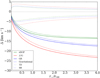Fig. 4. Predicted value of $\overline{\mathrm{\Delta }}$ as a function of the cluster radius in units of r500. The blue lines refer to the predictions computed assuming GR, the green lines refer to the sDGP predictions, and the red lines refer to f(R) gravity theory. For each colour, the dashed line shows the gravitational effect only, the dotted line the TD effect, the dot-dashed line the SB effect, and the solid line shows the combined effect.

7. Measuring the gravitational redshift

7.1. Correction of the phase-space diagram

To measure the gravitational redshift effect from the cluster member catalogue constructed in Sect. 3, we stacked all the data of the member galaxies (i.e. the transverse distances r_⊥, and line-of-sight velocities Δ) in a single phase-space diagram (Kim & Croft 2004; Wojtak et al. 2011). Figure 5 (top panel) shows the stacked line-of-sight velocity offset distributions for the member galaxies in the WH15 catalogue.

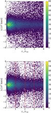Fig. 5. Phase-space diagram for the stacked member galaxy data of the clusters in the WH15 catalogue. The top panel shows the diagram before the correction procedure, while the bottom panel shows the background-corrected phase-space diagram. The colour bar shows the number of member galaxies we have in each bin. The bins have a size of 0.05 r500 × 50 km s−1. The vertical dashed red lines show the bins where we calculated the mean of the velocity distributions.

The phase-space diagram is affected by the contamination of the foreground and background galaxies, which are not gravitationally bound to any selected cluster, due to projection effects. We have to take into account only the galaxies that are within the cluster gravitational potential well to make a reliable measurement of the gravitational redshift. We followed the procedure described in Jimeno et al. (2015) to remove the contamination of foreground and background galaxies. The galaxies that did not belong to any cluster were considered statistically, once the data of all cluster member galaxies had been stacked into a single phase-space diagram (see Wojtak et al. 2007, for a detailed review on foreground and background galaxy removal techniques). Firstly, we split the phase-space distribution into bins of size 0.05 r₅₀₀ × 50 km s⁻¹. We assumed that the galaxies that lay in the stripes 3000 km s⁻¹ < |Δ|< 4000 km s⁻¹ belonged either to pure foreground or to pure background, as already described in Sect. 3. We selected the upper limit for galaxy line-of sight velocity of 4000 km s⁻¹ following the past literature work of Wojtak et al. (2011) and Sadeh et al. (2015). On the other hand, we made some tests changing the lower limit of 3000 km s⁻¹. Selecting the lower cut-off within the range 2000 km s⁻¹ < |Δ|< 3500 km s⁻¹, we obtained consistent results, within the errors, to the ones we present in Sect. 8.

We fitted a quadratic polynomial function, which depended on both Δ and r_⊥, to the points in both stripes. We used the interpolated model to correct the phase-space region where |Δ| was less than 3000 km s⁻¹, namely the region where the galaxies were gravitationally bound. The function f(r_⊥, Δ), which we used to model the phase-space region where the background and foreground galaxies lay, can be expressed as follows:

$$\begin{array}{c}\hfill f(r_{\perp },\mathrm{\Delta })=a{r}_{\perp }^2+b{\mathrm{\Delta }}^2+c{r}_{\perp }\mathrm{\Delta }+d\mathrm{\Delta }+e{r}_{\perp }+f,\end{array}$$(34)

where a, b, c, d, e, and f represent the free parameters of the model. We used a function that depended on both r_⊥ and Δ because, due to observational selections, we may observe more galaxies that are closer to us with respect to the cluster centre (i.e. negative Δ) than further away (i.e. positive Δ). Moreover, the possibility of finding galaxies that do not belong to the cluster increases with the distance from the cluster centre.

The bottom panel of Fig. 5 shows the background-corrected phase-space diagram. After removing the background, the phase-space diagram clearly shows the inner region where the gravitationally bound galaxies reside. Indeed, most of the galaxies in the foreground and background regions have been removed, proving that the background-correction method was successful. However, not all the contamination was removed because of the intrinsic uncertainties in the fitting. Thus, we took this error into account when we fitted the galaxy velocity distributions. In particular, we considered the mean rms as the error of the fitting procedure. In fact, the bottom panel of Fig. 5 shows that a certain amount of galaxies with a large velocity offset around r_⊥/r₅₀₀ ∼ 1 and 3 < r_⊥/r₅₀₀ < 4 was still present after the background correction. Nevertheless, in each bin of these parameter regions, we find at most one galaxy. This non-uniform background subtraction might be due to minor statistical uncertainties. To test the impact of this effect on the final results of our analysis, we measured again the gravitational redshift, considering only those galaxies with |Δ|< 2000 km s⁻¹, finding consistent results, within the errors, to the results presented in Sect. 8.

7.2. Fitting the data

We split the background-corrected phase-space diagrams into four equal bins of transverse distance to recover the gravitational redshift signal as a function of the transverse distance from the cluster centre. Each bin had a width of 1r₅₀₀, as shown in Fig. 5. We fitted the galaxy line-of-sight velocity distribution within each bin, in order to recover the mean of the distribution, $\overline{\mathrm{\Delta }}$. The mean value of the distribution was proportional to the intensity of the gravitational redshift effect and we expected a negative value, as explained in Sect. 4. We performed a Monte Carlo Markov chain (MCMC) statistical analysis to fit $\overline{\mathrm{\Delta }}$ within each bin. We modelled the velocity distribution as a double Gaussian function, which can be expressed as follows:

$$\begin{array}{c}\hfill f(\mathrm{\Delta })=\frac{\epsilon }{\sqrt{2\pi {\sigma }_1^2}}exp\left[\frac{{(\mathrm{\Delta }-\overline{\mathrm{\Delta }})}^2}{2{\sigma }_1^2}\right]+\frac{1-\epsilon }{\sqrt{2\pi {\sigma }_2^2}}exp\left[\frac{{(\mathrm{\Delta }-\overline{\mathrm{\Delta }})}^2}{2{\sigma }_2^2}\right],\end{array}$$(35)

where the two Gaussian functions have the same mean, $\overline{\mathrm{\Delta }}$. The relative normalisation of the two functions, ε, and their widths, σ₁ and σ₂, were considered as free parameters of the MCMC analysis, and marginalised over. The Bayesan fit was implemented by using a Gaussian likelihood, with flat priors on all the free model parameters. We considered the combination of two independent sources of errors: (i) the Poisson noise, and (ii) the error of the background-correction method. The quasi-Gaussian function given by Eq. (35) took into account the intrinsic non-Gaussian distributions of galaxy velocities in individual clusters and the different cluster masses.

8. Results

Figure 6 shows the velocity distributions in each bin of projected transverse distance. The figure shows the data of the binned background-corrected phase-space diagram, the associated error bars, and the best-fit models within each bin. We notice that the model systematically underestimates the data with low Δ at any distance from the centre. This is a feature that was present also in past literature works (Wojtak et al. 2011; Jimeno et al. 2015) and it does not significantly affect the final $\overline{\mathrm{\Delta }}$ estimation.

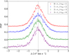Fig. 6. Velocity distributions of the WH15 cluster member galaxies in the four bins of projected transverse distance. These distributions were shifted vertically by an arbitrary amount (−0.2, 0, 0.2 and 0.35), for visual purposes. The coloured points represent the data of the binned background-corrected phase-space diagram and the error bars represent the Poisson noise combined with the error of the background-correction method. The solid lines and the shaded coloured areas show the best-fit models and their errors, respectively.

Figure 7 shows the comparison between the estimated $\overline{\mathrm{\Delta }}$ within each bin and the GR, f(R), and sDGP theoretical predictions, as a function of the transverse distance from the cluster centre. As it can be seen, we find a clear negative shift of the mean of the velocity distributions, as we expected from the theoretical analysis described in Sect. 4. As shown in Fig. 7, our measurements are in agreement, within the errors, with the predictions of GR and sDGP, while in marginal tension with f(R) predictions, though the disagreement is not statistically significant.

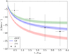Fig. 7. Comparison between the estimated $\overline{\mathrm{\Delta }}$ of the WH15 cluster member galaxies within each bin of transverse distance and the theoretical predictions from GR (solid blue line), f(R) (dotted red line), and sDGP (dash-dotted green line). The shaded coloured areas show the model errors that were caused by the fitting uncertainties on the cluster mass distribution, and the dispersion of the cluster redshifts. The black points show the estimated $\overline{\mathrm{\Delta }}$. The vertical error bars represent the range of the $\overline{\mathrm{\Delta }}$ parameter, containing 68% of the marginalised posterior probability, while the horizontal error bars show the dispersion of the galaxy transverse distances in a given bin.

The richness-mass scaling relation is a crucial element in this kind of analysis, since it can introduce systematic biases in the final constraints if not properly calibrated in the assumed gravity theory considered. In particular, the so-called fifth force, possibily arising from the new scalar degrees of freedom of modified gravity models, such as the f(R) scenario considered in this work, modifies the relation between the cluster masses and observable proxies (Terukina et al. 2014; Wilcox et al. 2015). To test the impact of this effect, we performed the full analysis again using Eqs. (6) and (22) from Mitchell et al. (2021) to compute the M₅₀₀ masses for each cluster in the f(R) strong field scenario. We find that the new M₅₀₀ values are, on average, about 15% higher than the corresponding masses estimated in GR, and the new gravitational redshift measurements are shifted, on average, by about 20% towards positive $\overline{\mathrm{\Delta }}$ values with respect to the results shown in Fig. 7. The results of this test are shown in Appendix A.3. These new results are within the estimated statistical uncertainties, and thus do not introduce dominant systematic effects for the current analysis. An accurate calibration of the mass-observable scaling relation in different modified gravity models will be mandatory for similar analyses on next-generation large cluster samples and will deserve a detailed study that is beyond the scope of the present paper.

We also measured the integrated gravitational redshift signal up to 4r₅₀₀, ${\overline{\mathrm{\Delta }}}_{\mathrm{int}}$, by considering all the cluster member galaxies in the background-corrected phase-space diagram shown in Fig. 5. We obtained ${\overline{\mathrm{\Delta }}}_{\mathrm{int}}=-11.4\pm 3.3$ km s⁻¹, which is in agreement, within the errors, with the expected value of −10 km s⁻¹ predicted in GR for clusters in the mass range of the WH15 cluster member catalogue.

We fitted the measured value of $\overline{\mathrm{\Delta }}$, shown in Fig. 7, to impose new constraints on the gravity theory and discriminate among the three different models considered. To do this, we modified the theoretical model given by Eq. (31), by changing the gravitational acceleration experienced by the photons inside the clusters. In practice, we multiplied the gravitational constant G by a constant α, which was considered as the free parameter of the fit. This simple model was accurate enough to take into account the modification of the gravitational force predicted by both the f(R) and sDGP models. By construction, α is equal to unity in GR theory, while α = 1.33 in the f(R) theory and α ≃ 0.85 in the sDGP model. We performed a MCMC analysis to fit the measured $\overline{\mathrm{\Delta }}$, using a Gaussian likelihood. It should be noted that this fitting procedure has never been implemented in past literature works.

Figure 8 shows the results of the MCMC analysis. We obtained α = 0.86 ± 0.25, with a reduced χ² = 0.23. The value of the reduced χ² indicates a possible overestimation of the measurement errors. The best-fit results confirm that our measurements are in agreement, within the error, with GR and sDGP predictions, while the f(R) model is marginally discarded at about 2σ. This result is consistent with past literature works that have already discarded the f(R) strong field scenario considered here (e.g. Terukina et al. 2014; Wilcox et al. 2015). Our result is also compliant with what has been found by Marulli et al. (2021) from a redshift-space distortion analysis of the two-point correlation function of the same cluster catalogue. On the other hand, this is in slight disagreement with the works of Wojtak et al. (2011) and Mpetha et al. (2021), whose results were consistent also with f(R). Nevertheless, as noted above, a proper self-consistent treatment of the richness-mass scaling relation in modified gravity models would be required to assess unbiased constraints. In fact, the analysis presented here provides robust constraints on GR predictions, for which the likelihood model calibration is accurate enough, given the current uncertainties. On the other hand, the comparison of our measurements with different gravity theories should be taken with caution, and no strong conclusions can be drawn in this respect.

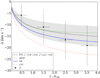Fig. 8. Best-fit model of $\overline{\mathrm{\Delta }}(r_{\perp }/r_{500})$ from MCMC (solid grey line) for the WH15 cluster member galaxies. The shaded grey area shows the 68% uncertainty on the posterior median. The theoretical predictions of GR (solid blue line), f(R) (dotted red line), and sDGP (dash-dotted green line) are shown for comparison.

9. Conclusions

In this work we tested the Einstein theory of GR by measuring the gravitational redshift effect in galaxy clusters, within the ΛCDM cosmological framework. To perform the gravitational redshift measurements, we constructed a new cluster member galaxy catalogue, as discussed in Sect. 3. Differently from past literature works, we used the average positions and redshifts of central galaxies to estimate the cluster centres. In Appendix A.1 we compare the results obtained with this choice to those obtained assuming the BCGs as the cluster centres. Following the method described by Kim & Croft (2004), we stacked the data of the cluster member galaxies in a single phase-space diagram and corrected them for the background and foreground galaxy contaminations, as explained in Sect. 7.1. We split the phase-space diagrams in four bins of transverse distances from the cluster centre, recovering the galaxy velocity distributions within them. We implemented an MCMC analysis, described in Sect. 7.2, to recover the shift of the mean of the velocity distributions, which was proportional to the gravitational redshift effect. We found a significant negative signal in all four of the bins of projected transverse distances from the cluster centre. Moreover, the signal becomes more negative as the distance from the centre increases, as expected. We recovered an integrated gravitational redshift signal of ${\overline{\mathrm{\Delta }}}_{\mathrm{int}}=-11.4\pm 3.3$ km s⁻¹ up to a distance of about 3 Mpc from the cluster centre. This value is in agreement with the expected value of approximately −10 km s⁻¹, predicted in GR for clusters in the same range of masses as those considered here. The error on this integrated signal is about 30% lower with respect to what was found in the previous works by Sadeh et al. (2015) and Mpetha et al. (2021).

We computed the theoretical gravitational redshift effect in three different gravity theories: GR, f(R), and sDGP. The gravitational redshift model predictions are shown in Fig. 4. We compared our measurements with theoretical predictions as a function of the transverse distance from the cluster centre. This comparison is shown in Fig. 7. We implemented a new statistical analysis method in order to discriminate among the different gravity theories, as described in Sect. 8. The free parameter of this analysis was α, which modelled the gravitational acceleration in different gravity theories (by construction, α is equal to unity in GR). We obtained α = 0.86 ± 0.25. This result is in agreement with GR and sDGP predictions, within the errors, while marginally inconsistent with the f(R) strong field model at about 2σ significance, in line with literature results (e.g. Terukina et al. 2014; Wilcox et al. 2015).

This work demonstrates that the peculiar velocity distribution of the cluster member galaxies provides a powerful tool to directly investigate the gravitational potentials within galaxy clusters and to impose new constraints on the gravity theory on megaparsec scales. Further investigations are necessary to corroborate the measurement method by exploiting cosmological simulations, especially at high redshifts, and to improve the modelling for both galaxy velocity distributions and gravitational redshift theoretical predictions. The model improvements are necessary to take into account the BCG proper motions, and to relax the assumption of the cluster spherical symmetry and the NFW density profile. Forecasting analyses are needed to compute the required number of clusters and associated member galaxies necessary to discriminate among different gravity theories with a high statistical significance. It will be useful to investigate the effects possibly caused by mixing data from different spectroscopic surveys, which can be done to increase the available statistics by jointly combining different data sets. Furthermore, it will be crucial to accurately calibrate the richness-mass scaling relation in different gravity models, to minimise the related systematic biases in the likelihood analysis.

To perform an even stronger test on GR, it will be necessary to reduce the measurement errors, which mainly depend on the number of cluster member galaxies available with spectroscopic redshift measurements. Large cluster and galaxy samples from upcoming missions will be crucial. In particular, the ESA Euclid mission⁶ (Laureijs et al. 2011; Amendola et al. 2018) will detect ∼2 × 10⁶ galaxy clusters up to z ∼ 2 with a spectroscopic identification of the cluster member galaxies (see e.g. Sartoris et al. 2016). The scientific exploitation of the Euclid cluster catalogues will be key to obtain definite constraints on the gravity theory from gravitaional redshifts inside galaxy clusters.

Acknowledgments

We thank the anonymous referee for the useful comments to improve the quality of the paper. We acknowledge the grants ASI n.I/023/12/0 and ASI n.2018-23-HH.0. LM acknowledges support from the grant PRIN-MIUR 2017 WSCC32. We acknowledge the use of computational resources from the parallel computing cluster of the Open Physics Hub (https://site.unibo.it/openphysicshub/en) at the Physics and Astronomy Department in Bologna.

References

Appendix A: Testing the systematic uncertainties in the analysis

In this appendix we describe the tests we conducted to investigate the effects on the gravitational redshift measurements of the various selections on the cluster member galaxies. Moreover, we discuss how our results change when we assume the BCG as the cluster centre, as done in past literature works by Wojtak et al. (2011), Jimeno et al. (2015) and Sadeh et al. (2015).

A.1. Assuming the BCG as the cluster centre

In this work, we used the average galaxy positions and redshifts to estimate the cluster centres. To investigate the impact of this choice on the measurement results, we repeated the analysis by assuming the BCG as the cluster centre, as done in past literature works. We constructed the cluster member catalogues by using the same selection criteria described in Sec. 3. When we estimated the cluster centre from the BCG, all the cluster member galaxies were selected all over again. The new set of member galaxies in the outer cluster region was different in this case, since galaxies near the edges of our selection could be either included or excluded, depending on the centre choice, according to the selection criteria described in Sec. 3. We obtained a cluster member catalogue with 3065 clusters and 46 819 cluster member galaxies.

We constructed the background-corrected phase-space diagrams as described in Sec. 7.1, in order to compare the results with those described in Sec. 8. Then, we fitted the galaxy velocity distributions to retrieve the gravitational redshift signal as a function of the transverse distance from the cluster centre. We also estimated the α parameter by fitting the measured $\overline{\mathrm{\Delta }}$, using the same fitting procedure described in Sec. 8.

Figure A.1 shows the MCMC results, comparing the estimated $\overline{\mathrm{\Delta }}$ assuming the BCG as the cluster centre within each distance bin and the theoretical predictions from GR, f(R), and sDGP as functions of the transverse distance from the cluster centre. Figure A.1 shows that the measurements in the outermost bins are in agreement with the theoretical models, while those in the inner bins are not, showing positive values of the mean of the galaxy velocity distribution. We interpret this result in the inner bins as mainly caused by two effects. Firstly, the BCG peculiar velocities cause a positive shift of $\overline{\mathrm{\Delta }}$, as demonstrated by Kaiser (2013), which is similar to the TD effect, but less intense. This effect was not included in the theoretical model, described in Sec. 4, because it was expected to be a second-order effect. Moreover, we did not have any information about the BCG peculiar velocities. Further investigations are necessary to understand the real impact of the BCG peculiar motions. Secondly, the BCGs might be misidentificated, due to the surface brightness modulation and velocity effects. In cases where the true BCG is not identified, we may erroneously consider a hot-population object as the cluster centre. Thus, these galaxies may be located at a non-negligible distance from the centre of the cluster gravitational potential well. Thus, the BCG false identification might cause a positive shift of the mean of the velocity distribution. A similar result was obtained by Jimeno et al. (2015) analysing the WHL12 cluster sample and assuming the BCG as the cluster centre. Jimeno et al. (2015) found marginally positive values of $\overline{\mathrm{\Delta }}$ in all the analysed bins of transverse distance from the cluster centre, up to 7 Mpc.

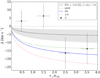Fig. A.1. Best-fit model of $\overline{\mathrm{\Delta }}$ from MCMC (solid grey line) for the analysed cluster member galaxies, which are identified assuming the BCG as the cluster centre. The symbols are the same as in Fig. A.3.

In this case, we obtained $\alpha =0.{32}_{-0.20}^{+0.25}$ with a reduced χ² equal to 1.78. The best-fit model is marginally inconsistent with any gravity theory we analysed, and it is almost compatible with zero. The error on the α parameter is asymmetric because we imposed, as a prior, that α had to be greater than zero (if α = 0, we do not have a gravitational force, while α < 0 would imply an anti-gravity force).

Hence, we conclude that, in this case, we do not have a reliable α estimation due to the BCG misidentification and the peculiar velocity effects, which are not taken into account in the model. Further investigations are necessary to improve the modelling when the BCG position is assumed as the cluster centre.

A.2. Testing the selections

When we searched for the cluster member galaxies, we applied a number of selections, which are described in Sec. 3. Here we discuss the impact of these choices on the gravitational redshift measurements.

A.2.1. Selection of the cluster member galaxies

In the analysis presented in this work, we considered only the clusters that had at least four associated member galaxies. We did this following Wojtak et al. (2011) and Jimeno et al. (2015), who made a similar selection. This choice was useful to mitigate the problem of false cluster identification. We tested the effect of this selection by measuring the gravitational redshift in the phase-space diagrams constructed by changing the minimum number of cluster associated member galaxies. We notice that if the minimum number increases above six, the statistics becomes too low, and the measurement cannot be performed due to the too small number of remaining clusters, which increases the Poisson noise in the velocity distributions. Considering a number of members in the range between three and six, the final results are not significantly affected and remain in agreement with those described in Sec. 8. On the other hand, if the minimum number of cluster member galaxies is less than three, the cluster false identification significantly affects the measurement causing a positive shift of the velocity distribution mean.

A.2.2. Minimum number of galaxies used to compute the centre

A second choice we made in our analysis was to select only the clusters whose centres could be computed with at least three member galaxies. We made this choice to select only clusters whose average redshifts had an error that was reduced by at least 50% with respect to the BCG spectroscopic redshift error. In fact, when we computed the velocity distributions, the centre redshift error propagated to all the redshifts of the cluster member galaxies. This is a major issue, especially for the clusters with a large number of members. We made several tests by arbitrarily increasing the redshift error of the cluster centre, up to 5 × 10⁻³. We notice that, as the error increases, the velocity distributions have an increasing larger positive shift of the mean. Further analyses are necessary to investigate this effect. Moreover, we notice that if the number of member galaxies used to estimate the centres increases above five, the statistics becomes too low, which does not allow us to obtain any sufficiently accurate measure. On the other hand, if this number is less than three, the results are not statistically distinguishable from those obtained when considering the BCG as the cluster centre (these measurements are described in Sec. A.1). For clusters whose average centre positions were computed with three to five galaxies, the final results do not vary significantly from those described in Sec. 8.

A.2.3. Cluster redshift range

In our analysis, we selected only the clusters that had a redshift smaller than 0.5, to mitigate the problem of false cluster identifications, and to mitigate the possible impact of the assumed cosmological model on the measurements. In order to test this selection, we measured the gravitational redshift by changing the cluster redshift cut-off. When we considered the low-redshift clusters with z < 0.2, the lack of statistics prevented us from obtaining any measurement. We also tested the analysis up to z = 0.6. In this case the final measurements did not vary significantly from those described in Sec. 8. Further studies are necessary to investigate the method at higher redshifts, by exploiting cosmological simulations, to quantify how gravitational redshift theoretical predictions are affected by the redshift dependence of cosmological parameters.

A.2.4. Mass selection

A further selection we applied in our analysis was to consider only the clusters that had masses above 1.5 × 10¹⁴ M_⊙, in order to mitigate the problem of false cluster identification, as described in Sec. 3. To investigate the impact of also including lower-mass clusters, we measured the gravitational redshift as a function of the cluster mass. We split the cluster member catalogue in four sub-samples covering different cluster mass ranges. We did not take into account clusters with masses lower than 3 × 10¹³ M_⊙, because for those clusters, the richness-mass relation was not calibrated, as described in Sec. 2.1. For each sub-sample we constructed the background-corrected phase-space diagram and measured the integrated gravitational redshift ${\overline{\mathrm{\Delta }}}_{\mathit{int}}$ signal up to a transverse distance from the cluster centre of 4r₅₀₀.

Figure A.2 shows the comparison between the estimated integrated signal ${\overline{\mathrm{\Delta }}}_{\mathit{int}}$ up to 4r₅₀₀, within each sub-sample, and the GR, f(R), and sDGP predictions. The figure shows that the measurements at M₅₀₀ ≳ 2 × 10¹⁴ M_⊙ are in agreement, within the errors, with the GR and sDGP theoretical predictions. Moreover, in this mass range, the integrated signal up to 4r₅₀₀ becomes more negative as the cluster mass increases, as expected. On the other hand, the ${\overline{\mathrm{\Delta }}}_{\mathit{int}}$ value for clusters with average mass of about 1.5 × 10¹⁴ M_⊙ is positive and it is not in agreement with any prediction, while the ${\overline{\mathrm{\Delta }}}_{\mathit{int}}$ measurement in the lowest mass range is again in agreement with all theoretical predictions. The positive value of ${\overline{\mathrm{\Delta }}}_{\mathit{int}}$ is probably caused by a high percentage of falsely identified clusters in this mass range.

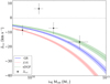Fig. A.2. Comparison between the estimated integrated gravitational redshift signal ${\overline{\mathrm{\Delta }}}_{\mathit{int}}$ up to 4r500 and the theoretical predictions from GR (solid blue line), f(R) (dotted red line), and sDGP (dash-dotted green line) as a function of the cluster mass. The shaded coloured areas show the model errors, while the black points show the estimated ${\overline{\mathrm{\Delta }}}_{\mathit{int}}$. The vertical error bars represent the range of the ${\overline{\mathrm{\Delta }}}_{\mathit{int}}$ parameter containing 68% of the marginalised posterior probability, while the horizontal error bars show the dispersion of the cluster masses in a given bin.

To investigate the impact of the mass selection on the measurements, we stacked all the clusters with masses above 3 × 10¹³ M_⊙ in a single background-corrected phase-space diagram, and measured the gravitational redshift effect as a function of the transverse distance from the cluster centre. We split the phase-space diagrams into four bins of width equal to r₅₀₀, as done in Sec. 8. We also fittedthe measured $\overline{\mathrm{\Delta }}$ with the procedure described in Sec. 8, to constrain the α parameter.

Figure A.3 shows the result of the MCMC and the comparison between the estimated $\overline{\mathrm{\Delta }}$ within each bin and the GR, f(R), and sDGP theoretical predictions. Figure A.3 shows that the measurements are in marginal agreement only with the sDGP predictions in all four of the bins, which is different from the mass-selected cluster member sample considered in the analysis of this work (see Fig. 7). We interpret this result as possibly caused by the falsely identified low-mass clusters. In this case we obtained a value of α equal to 0.51 ± 0.19, with a reduced χ² of 0.07. This value is marginally inconsistent with the estimation obtained from the mass-selected cluster member sample, which is 0.86 ± 0.25 (see Fig. 8).

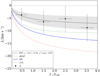Fig. A.3. Best-fit model of $\overline{\mathrm{\Delta }}$ from the MCMC (solid grey line) for all the clusters with mass above 3 × 1013 M⊙. The shaded grey area shows the 68% uncertainty on the posterior median. The theoretical predictions as functions of the transverse distance from the cluster centre from the GR (solid blue line), f(R) (dotted red line), and sDGP (dash-dotted green line) are shown for comparison.

A.3. Cosmological dependence of the relation between the cluster masses and observable proxies

As described in Sec. 8, we tested the impact of modifying the relation between the cluster masses and observable proxies, when we assumed f(R) gravity theory. We computed the new M₅₀₀ masses for each cluster in the f(R) strong field scenario following Mitchell et al. (2021). For each cluster we also computed the radius, r₅₀₀, and the concentration parameter, c₅₀₀. Then we performed the full statistical analysis again. Figure A.4 shows the comparison between ${\overline{\mathrm{\Delta }}}_{f(R)}$, which are the results of this test, and ${\overline{\mathrm{\Delta }}}_{\mathit{GR}}$, which are the measurements also shown in Figs. 7 and 8. The f(R) theoretical predictions were computed considering the new M₅₀₀ values. As shown in the figure, the ${\overline{\mathrm{\Delta }}}_{f(R)}$ measurements are shifted towards positive values with respect to ${\overline{\mathrm{\Delta }}}_{\mathit{GR}}$, as discussed in Sec. 8.

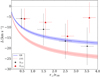Fig. A.4. Comparison between the $\overline{\mathrm{\Delta }}$ values computed with the scaling relation estimated in the f(R) strong field scenario, ${\overline{\mathrm{\Delta }}}_{f(R)}$ (red triangles), and the ones assuming the reference scaling relation considered in this paper, ${\overline{\mathrm{\Delta }}}_{\mathit{GR}}$ (black points). The former values are shifted horizontally by 0.1r⊥/r500, for visual purposes. The theoretical f(R) predictions were computed using the M500 values obtained from the f(R) scaling relation. The shaded coloured areas show the theoretical uncertainties caused by the fitting uncertainties on the cluster mass distribution, and the dispersion of the cluster redshifts. The vertical error bars represent the range of the $\overline{\mathrm{\Delta }}$ parameter containing 68% of the marginalised posterior probability, while the horizontal error bars show the dispersion of the galaxy transverse distances in each given bin.

All Tables

All Figures

	Fig. 1. Redshift distribution of the selected galaxies. The blue histogram represents the galaxy redshift distribution of the Legacy Survey, while the red histogram shows the distribution of BOSS and eBOSS.
In the text

Fig. 2. Redshift (top panel) and mass distribution (bottom panel) of the selected cluster sample. The solid blue histograms represent the distributions of all WL15 clusters within the redshift and mass ranges where the richness-mass relation was calibrated. The yellow histograms show the distributions of the clusters with mass above 1.5 × 1014 M⊙, while the green histograms show the distributions of the clusters with z < 0.5. The dashed purple histograms show the distributions of the clusters that have at least four associated galaxies. Finally, the red histograms represent the distributions of the final selected cluster sample.

In the text

Fig. 3. Angular maps around four galaxy clusters of the selected sample. The black points represent the cluster member galaxies, while the red squares show the positions of the field galaxies. The gold diamond shows the cluster centres and the cyan star represents the cluster BCGs. The dashed green circle indicates the cluster r500 radii. The arrows show the galaxy line-of-sight velocities with respect to the cluster centres. The arrows pointing upwards (downwards) represent positive (negative) velocities. The objects are representative examples of four different cluster types: a low-redshift massive cluster with a large number of identified galaxy members (top left panel); a high-redshift small cluster, though with a sufficient number of members (top right panel); an isolated cluster with only a few identified members (bottom left panel); and two small close clusters (bottom right panel).

In the text

Fig. 4. Predicted value of $\overline{\mathrm{\Delta }}$ as a function of the cluster radius in units of r500. The blue lines refer to the predictions computed assuming GR, the green lines refer to the sDGP predictions, and the red lines refer to f(R) gravity theory. For each colour, the dashed line shows the gravitational effect only, the dotted line the TD effect, the dot-dashed line the SB effect, and the solid line shows the combined effect.

In the text

Fig. 5. Phase-space diagram for the stacked member galaxy data of the clusters in the WH15 catalogue. The top panel shows the diagram before the correction procedure, while the bottom panel shows the background-corrected phase-space diagram. The colour bar shows the number of member galaxies we have in each bin. The bins have a size of 0.05 r500 × 50 km s−1. The vertical dashed red lines show the bins where we calculated the mean of the velocity distributions.

In the text

Fig. 6. Velocity distributions of the WH15 cluster member galaxies in the four bins of projected transverse distance. These distributions were shifted vertically by an arbitrary amount (−0.2, 0, 0.2 and 0.35), for visual purposes. The coloured points represent the data of the binned background-corrected phase-space diagram and the error bars represent the Poisson noise combined with the error of the background-correction method. The solid lines and the shaded coloured areas show the best-fit models and their errors, respectively.

In the text

Fig. 7. Comparison between the estimated $\overline{\mathrm{\Delta }}$ of the WH15 cluster member galaxies within each bin of transverse distance and the theoretical predictions from GR (solid blue line), f(R) (dotted red line), and sDGP (dash-dotted green line). The shaded coloured areas show the model errors that were caused by the fitting uncertainties on the cluster mass distribution, and the dispersion of the cluster redshifts. The black points show the estimated $\overline{\mathrm{\Delta }}$. The vertical error bars represent the range of the $\overline{\mathrm{\Delta }}$ parameter, containing 68% of the marginalised posterior probability, while the horizontal error bars show the dispersion of the galaxy transverse distances in a given bin.

In the text

	Fig. 8. Best-fit model of $\overline{\mathrm{\Delta }}(r_{\perp }/r_{500})$ from MCMC (solid grey line) for the WH15 cluster member galaxies. The shaded grey area shows the 68% uncertainty on the posterior median. The theoretical predictions of GR (solid blue line), f(R) (dotted red line), and sDGP (dash-dotted green line) are shown for comparison.
In the text

	Fig. A.1. Best-fit model of $\overline{\mathrm{\Delta }}$ from MCMC (solid grey line) for the analysed cluster member galaxies, which are identified assuming the BCG as the cluster centre. The symbols are the same as in Fig. A.3.
In the text

Fig. A.2. Comparison between the estimated integrated gravitational redshift signal ${\overline{\mathrm{\Delta }}}_{\mathit{int}}$ up to 4r500 and the theoretical predictions from GR (solid blue line), f(R) (dotted red line), and sDGP (dash-dotted green line) as a function of the cluster mass. The shaded coloured areas show the model errors, while the black points show the estimated ${\overline{\mathrm{\Delta }}}_{\mathit{int}}$. The vertical error bars represent the range of the ${\overline{\mathrm{\Delta }}}_{\mathit{int}}$ parameter containing 68% of the marginalised posterior probability, while the horizontal error bars show the dispersion of the cluster masses in a given bin.

In the text

Fig. A.3. Best-fit model of $\overline{\mathrm{\Delta }}$ from the MCMC (solid grey line) for all the clusters with mass above 3 × 1013 M⊙. The shaded grey area shows the 68% uncertainty on the posterior median. The theoretical predictions as functions of the transverse distance from the cluster centre from the GR (solid blue line), f(R) (dotted red line), and sDGP (dash-dotted green line) are shown for comparison.

In the text

Fig. A.4. Comparison between the $\overline{\mathrm{\Delta }}$ values computed with the scaling relation estimated in the f(R) strong field scenario, ${\overline{\mathrm{\Delta }}}_{f(R)}$ (red triangles), and the ones assuming the reference scaling relation considered in this paper, ${\overline{\mathrm{\Delta }}}_{\mathit{GR}}$ (black points). The former values are shifted horizontally by 0.1r⊥/r500, for visual purposes. The theoretical f(R) predictions were computed using the M500 values obtained from the f(R) scaling relation. The shaded coloured areas show the theoretical uncertainties caused by the fitting uncertainties on the cluster mass distribution, and the dispersion of the cluster redshifts. The vertical error bars represent the range of the $\overline{\mathrm{\Delta }}$ parameter containing 68% of the marginalised posterior probability, while the horizontal error bars show the dispersion of the galaxy transverse distances in each given bin.

In the text

References

- Abazajian, K. N., Adelman-McCarthy, J. K., Agüros, M. A., et al. 2009, ApJS, 182, 543 [NASA ADS] [CrossRef] [Google Scholar]
- Ahn, C. P., Alexandroff, R., Prieto, C. A., et al. 2014, ApJS, 211, 17 [NASA ADS] [CrossRef] [Google Scholar]
- Ahumada, R., Prieto, C. A., Almeida, A., et al. 2020, ApJS, 249, 3 [Google Scholar]
- Aihara, H., Prieto, C. A., An, D., et al. 2011, ApJS, 193, 29 [NASA ADS] [CrossRef] [Google Scholar]
- Alam, S., Albareti, F. D., Prieto, C. A., et al. 2015, ApJS, 219, 12 [NASA ADS] [CrossRef] [Google Scholar]
- Amendola, L., Appleby, S., Avgoustidis, A., et al. 2018, Liv. Rev. Relativ., 21, 2 [NASA ADS] [CrossRef] [Google Scholar]
- Baldry, I. K. 2018, Reinventing the Slide Rule for Redshifts: the Case for Logarithmic Wavelength Shift [Google Scholar]
- Beutler, F., Saito, S., Seo, H.-J., et al. 2014, MNRAS, 443, 1065 [NASA ADS] [CrossRef] [Google Scholar]
- Cai, Y.-C., Kaiser, N., Cole, S., & Frenk, C. 2017, MNRAS, 468, 1981 [NASA ADS] [CrossRef] [Google Scholar]
- Cappi, A. 1995, A&A, 301, 6 [NASA ADS] [Google Scholar]
- Clerc, N., Kirkpatrick, C. C., Finoguenov, A., et al. 2020, MNRAS, 497, 3976 [NASA ADS] [CrossRef] [Google Scholar]
- Dawson, K. S., Kneib, J.-P., Percival, W. J., et al. 2016, AJ, 151, 44 [Google Scholar]
- Dawson, K. S., Schlegel, D. J., Ahn, C. P., et al. 2013, AJ, 145, 10 [Google Scholar]
- Deffayet, C. 2001, Phys. Lett. B, 502, 199 [NASA ADS] [CrossRef] [Google Scholar]
- Duffy, A. R., Schaye, J., Kay, S. T., & Dalla Vecchia, C. 2008, MNRAS, 390, L64 [Google Scholar]
- Dvali, G., Gabadadze, G., & Porrati, M. 2000, Phys. Lett. B, 485, 208 [Google Scholar]
- Eisenstein, D. J., Annis, J., Gunn, J. E., et al. 2001, AJ, 122, 2267 [Google Scholar]
- Fang, W., Wang, S., Hu, W., et al. 2008, Phys. Rev. D, 78, 103509 [NASA ADS] [CrossRef] [Google Scholar]
- Hansen, S. M., Sheldon, E. S., Wechsler, R. H., & Koester, B. P. 2009, ApJ, 699, 1333 [NASA ADS] [CrossRef] [Google Scholar]
- Hao, J., McKay, T. A., Koester, B. P., et al. 2010, ApJS, 191, 254 [Google Scholar]
- Jimeno, P., Broadhurst, T., Coupon, J., Umetsu, K., & Lazkoz, R. 2015, MNRAS, 448, 1999 [NASA ADS] [CrossRef] [Google Scholar]
- Kaiser, N. 2013, MNRAS, 435, 1278 [NASA ADS] [CrossRef] [Google Scholar]
- Kim, Y.-R., & Croft, R. A. C. 2004, ApJ, 607, 164 [NASA ADS] [CrossRef] [Google Scholar]
- Laureijs, R., Amiaux, J., Arduini, S., et al. 2011, ArXiv e-prints [arXiv:1110.3193] [Google Scholar]
- Łokas, E. L., & Mamon, G. A. 2001, MNRAS, 321, 155 [CrossRef] [Google Scholar]
- Marulli, F., Veropalumbo, A., & Moresco, M. 2016, Astron. Comput., 14, 35 [Google Scholar]
- Marulli, F., Veropalumbo, A., García-Farieta, J. E., et al. 2021, ApJ, 920, 13 [Google Scholar]
- Mitchell, M. A., Arnold, C., & Li, B. 2021, MNRAS, 502, 6101 [NASA ADS] [CrossRef] [Google Scholar]
- Miyazaki, S., Oguri, M., Hamana, T., et al. 2017, PASJ, 70, S27 [NASA ADS] [Google Scholar]
- Montero-Dorta, A. D., & Prada, F. 2009, MNRAS, 399, 1106 [NASA ADS] [CrossRef] [Google Scholar]
- Moresco, M., & Marulli, F. 2017, MNRAS, 471, L82 [NASA ADS] [CrossRef] [Google Scholar]
- Mpetha, C. T., Collins, C. A., Clerc, N., et al. 2021, MNRAS, 503, 669 [NASA ADS] [CrossRef] [Google Scholar]
- Navarro, J. F., Frenk, C. S., & White, S. D. M. 1995, MNRAS, 275, 720 [NASA ADS] [CrossRef] [Google Scholar]
- Nicolis, A., & Rattazzi, R. 2004, J. High Energy Phys., 2004, 059 [CrossRef] [Google Scholar]
- Planck Collaboration VI. 2020, A&A, 641, A6 [NASA ADS] [CrossRef] [EDP Sciences] [Google Scholar]
- Rykoff, E. S., Rozo, E., Busha, M. T., et al. 2014, ApJ, 785, 104 [Google Scholar]
- Sadeh, I., Feng, L. L., & Lahav, O. 2015, Phys. Rev. Lett., 114, 071103 [NASA ADS] [CrossRef] [Google Scholar]
- Sartoris, B., Biviano, A., Fedeli, C., et al. 2016, MNRAS, 459, 1764 [Google Scholar]
- Schmidt, F. 2010, Phys. Rev. D, 81, 103002 [NASA ADS] [CrossRef] [Google Scholar]
- Sotiriou, T. P., & Faraoni, V. 2010, Rev. Mod. Phys., 82, 451 [NASA ADS] [CrossRef] [Google Scholar]
- Starobinsky, A. 1980, Phys. Lett. B, 91, 99 [NASA ADS] [CrossRef] [Google Scholar]
- Strauss, M. A., Weinberg, D. H., Lupton, R. H., et al. 2002, AJ, 124, 1810 [Google Scholar]
- Terukina, A., Lombriser, L., Yamamoto, K., et al. 2014, J. Cosmol. Astropart. Phys., 2014, 013 [CrossRef] [Google Scholar]
- Wen, Z., & Han, J. 2015, ApJ, 807, 178 [NASA ADS] [CrossRef] [Google Scholar]
- Wen, Z. L., Han, J. L., & Liu, F. S. 2012, ApJS, 199, 34 [Google Scholar]
- Wilcox, H., Bacon, D., Nichol, R. C., et al. 2015, MNRAS, 452, 1171 [NASA ADS] [CrossRef] [Google Scholar]
- Wojtak, R., Lokas, E. L., Mamon, G. A., et al. 2007, A&A, 466, 437 [NASA ADS] [CrossRef] [EDP Sciences] [Google Scholar]
- Wojtak, R., Hansen, S. H., & Hjorth, J. 2011, Nature, 477, 567 [NASA ADS] [CrossRef] [Google Scholar]
- York, D. G., Adelman, J., Anderson, J. E. J., et al. 2000, AJ, 120, 1579 [Google Scholar]
- Zhao, H., Peacock, J. A., & Li, B. 2013, Phys. Rev. D, 88, 043013 [NASA ADS] [CrossRef] [Google Scholar]