| Issue |
A&A
Volume 669, January 2023
|
|
|---|---|---|
| Article Number | A10 | |
| Number of page(s) | 10 | |
| Section | Galactic structure, stellar clusters and populations | |
| DOI | https://doi.org/10.1051/0004-6361/202244194 | |
| Published online | 21 December 2022 | |
Did the Milky Way just light up? The recent star formation history of the Galactic disc⋆
1
Max-Planck-Institut für Astronomie, Königstuhl 17, 69117 Heidelberg, Germany
e-mail: This email address is being protected from spambots. You need JavaScript enabled to view it.
2
Canadian Institute for Theoretical Astrophysics, University of Toronto, 60 St. George Street, Toronto, ON M5S 3H8, Canada
3
Department of Astronomy and Astrophysics, University of Toronto, 50 St. George Street, Toronto, ON M5S 3H4, Canada
Received:
6
June
2022
Accepted:
21
September
2022
Abstract
We map the stellar age distribution (≲1 Gyr) across a 6 kpc × 6 kpc area of the Galactic disc in order to constrain our Galaxy’s recent star formation history. Our modelling draws on a sample that encompasses all presumed disc O-, B-, and A-type stars (∼500 000 sources) with G < 16. To be less sensitive to reddening, we did not forward-model the detailed CMD distribution of these stars; instead, we forward-modelled the K-band absolute magnitude distribution, n(MK), among stars with MK < 0 and Teff > 7000 K at certain positions x in the disc as a step function with five age bins, b(τ | x, α), logarithmically spaced in age from τ = 5 Myr to τ ∼ 1 Gyr. Given a set of isochrones and a Kroupa initial mass function, we sampled b(τ | x, α) to maximise the likelihood of the data n(MK | x, α), accounting for the selection function. This results in a set of mono-age stellar density maps across a sizeable portion of the Galactic disc. These maps show that some, but not all, spiral arms are reflected in overdensities of stars younger than 500 Myr. The maps of the youngest stars (< 10 Myr) trace major star-forming regions. The maps at all ages exhibit an outward density gradient and distinct spiral-like spatial structure, which is qualitatively similar on large scales among the five age bins. When summing over the maps’ areas and extrapolating to the whole disc, we find an effective star formation rate over the last 10 Myr of ≈ 3.3 M⊙ yr−1, higher than previously published estimates that had not accounted for unresolved binaries. Remarkably, our stellar age distribution implies that the star formation rate has been three times lower throughout most of the last Gyr, having risen distinctly only in the very recent past. Finally, we used TNG50 simulations to explore how justified the common identification of local age distribution with global star formation history is: we find that the global star formation rate at a given radius in Milky Way-like galaxies is approximated within a factor of ∼1.5 by the young age distribution within a 6 kpc × 6 kpc area near R⊙.
Key words: stars: early-type / Galaxy: structure / Galaxy: disk
Full Table 1 is only available at the CDS via anonymous ftp to cdsarc.cds.unistra.fr (130.79.128.5) or via https://cdsarc.cds.unistra.fr/viz-bin/cat/J/A+A/669/A10
© The Authors 2022
 Open Access article, published by EDP Sciences, under the terms of the Creative Commons Attribution License (https://creativecommons.org/licenses/by/4.0), which permits unrestricted use, distribution, and reproduction in any medium, provided the original work is properly cited.
This article is published in open access under the Subscribe-to-Open model.
Open access funding provided by Max Planck Society.
1. Introduction
Galaxies are fundamentally shaped by their star formation history. At any given epoch, the star formation rate (SFR) determines the population of massive, short-lived stars that regulate and change the composition and energetics of the interstellar medium (ISM). The SFR sets the rate at which the ISM is dispersed through galactic winds or locked away into long-lived, low-mass stars. It correlates with the nuclear activity of galaxies and the growth of stellar mass throughout cosmic time (Madau et al. 1996; Bouwens et al. 2011). Finally, the SFR is a fundamental input and observational constraint for galaxy evolution models (Chiappini et al. 1997; Kauffmann & Haehnelt 2000; de Rossi et al. 2009), again because it sets both the level of massive star feedback and the rate at which gas and dust are depleted.
In external unresolved galaxies the SFR is most often determined via a wide range of proxy measurements (see e.g., Kennicutt & Evans 2012). In the Milky Way, one can – at least in principle – count up the young stars. Low-mass stars can be discerned as being young if they have not yet reached the main sequence; massive stars can be discerned as young by their position in the colour-magnitude diagram (CMD), or simply by the fact that they are short-lived. However, not all stars can readily be recognised as young. Therefore, any such counting exercise must account for the fraction of the stellar mass function enclosed in such a census.
For nearby (d ≲ 500 pc) molecular clouds in the Milky Way, nearly complete lists of young stellar objects (YSOs) are available, the ages of which (t) can be derived by measuring their CMD positions or infrared excesses. The SFR is therefore given by ⟨Ṁ∗⟩ = NYSO ⟨MYSO⟩/t, where ⟨M*⟩ is the mean mass of YSOs and is usually assumed to be ⟨M*⟩ = 0.5 M⊙ (see e.g., Lada et al. 2010). In the local group, analogous SFR estimates have been based on the CMD position of massive luminous stars. For example, Williams et al. (2011) have applied CMD fitting techniques to reconstruct spatially resolved maps of the stellar age distribution in nearby galaxies.
The ‘current’ SFR of the Milky Way has been estimated by various groups over the last decade, for instance by Robitaille & Whitney (2010), Chomiuk & Povich (2011), and Licquia & Newman (2015). Specifically, Robitaille & Whitney (2010) used the census of YSOs from Robitaille et al. (2008, hereafter R08) to construct a population synthesis model for YSOs in the Galaxy, applied the same observational constraints as for the R08 census, and varied the model SFR such that the number of detected synthetic YSOs matched the observed number. They inferred a global SFR (across the entire Milky Way) of 0.68–1.45 M⊙ yr−1. Chomiuk & Povich (2011) normalised various estimates for the Galactic SFR to the same initial mass function (IMF) and population synthesis models across methods, and estimated ⟨Ṁ∗⟩ = 1.9 ± 0.4 M⊙ yr−1. Licquia & Newman (2015) revisited this work and estimated ⟨Ṁ∗⟩ = 1.65 ± 0.19 M⊙ yr−1 by combining previous measurements from the literature using a hierarchical Bayesian statistical method.
A conceptual limitation of such analyses is the identification of a measured age distribution of stars in a Galactic neighbourhood with the local or global star formation history of the Milky Way, for two reasons. First, young stars that are now seen in a modest volume (say, a few 100 pc) co-rotating with the Sun were not necessarily born within that volume. Second, we know from external disc galaxies that the instantaneous SFR varies dramatically as a function of position within a galaxy (see e.g., Fig. 1 in Kreckel et al. 2018, for a recent illustration); therefore, the extrapolation of a local census of young stars to a galaxy-wide SFR may be far off. To acknowledge this crucial distinction, but not completely discard traditional terminology, we use the term effective star formation rate for the quantity that is naively inferred from the age distribution. In addition, the SFR of galaxies may vary on short time scales, so any estimate of Ṁ∗ ∼ M∗(< Δt)/Δt will depend on the age range Δt of the young stars considered.
In this study, we set out to model and determine the age distribution over a substantive fraction (6 × 6 kpc around the Sun) of the Galactic disc, using upper main sequence, i.e. OB(A), stars. To do this, we devised and applied a non-parametric model1 for the age distribution of stars, which predicts their absolute magnitude distribution via isochrones. These predictions are then compared to OB(A) stars across many spatial patches in the Galactic disc, resulting in age-resolved spatial maps of stars younger than 1 Gyr. On that basis, we explored to what extent the modelled age distribution and its effective SFR reflect the actual disc star formation history of the Milky Way. Recently, Ruiz-Lara et al. (2020) made a comprehensive estimate of the age distribution of Galactic disc stars within 2 kpc by modelling Gaia DR2 colour–magnitude diagrams. However, their focus was on 0.5–10 Gyr timescales as opposed to the younger populations that we study here. Our analysis draws in the sample of massive stars from Zari et al. (2021), which we describe in Sect. 2. We lay out our methodology in Sect. 3. Our results, presented in Sect. 4, show a rapid increase in star formation rate compared to previous years, which could be related to the presence of numerous massive star-forming regions in the area considered. We discuss our results and summarise them in Sect. 5.
2. Data: Luminous young disc stars
The sample that we used in this study consists of ∼500 000 OB(A) stars in the ‘filtered’ sample presented in Zari et al. (2021, hereafter Z21). The sample was selected by combining Gaia EDR3 photometry and astrometry and 2MASS photometry by applying the following criteria. First, Z21 selected sources brighter than G = 16 mag and with absolute magnitude in the 2MASS Ks band MK < 0 mag, which roughly corresponds to a late B-type star. Then, they applied several cuts (described in Sect. 2.1 of Z21, Eqs. (2)–(5)) in colour–colour space to exclude bright red giant-branch and asymptotic giant-branch stars. To clean the sample from spurious astrometric solutions, they removed sources with astrometric fidelity < 0.9 (Rybizki et al. 2022). Finally, they selected sources in the Galactic disc that are and remain near the disc midplane, i.e. with |z|< 300 pc, and that belong to a low-velocity dispersion component in the vertical direction (identified with a Gaussian mixture model; see Sect. 4.2 of Zari et al. (2021). The latter condition was used to exclude stars with large vertical motions that point to a sample contamination by old, hot stars.
The Z21 sample extends to distances of ∼5 kpc from the Sun (Fig. 1, left). However, in this study we focused on a 6 kpc × 6 kpc region of the Galactic disc (centred on the Sun, shown in Fig. 1, right), where we can reasonably assume that our sample, is complete. To derive our spatially resolved SFR map of the Galactic disc, we divided our volume into 256 spaxels of different sizes, each containing the same number of stars (∼1000). We modelled the magnitude distribution of the sources in each spaxel, as described in the next section.
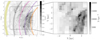 |
Fig. 1. Density distribution of the filtered sample of massive hot stars from Zari et al. (2021). In the left panel, the coloured lines represent the spiral arm locations derived by Reid et al. (2019). The right panel highlights the 6 × 6 kpc region considered in this study. Such region is divided in ‘spaxels’ of different sizes, each containing the same number of sources. In both panels, the Sun is in X, Y = (0, 0). |
3. Modelling the stellar age distribution
Ideally, we would like to model the observed colour-magnitude distribution of our sample stars in various spaxels to constrain their age distribution. However, this would require detailed star-by-star de-reddening, which would be difficult if not impossible (however, see e.g., Ruiz-Lara et al. 2020). Therefore, we resorted to modelling a more restricted set of observables centred on the near-infrared K band, which is less affected by extinction; we modelled the distribution of absolute magnitudes MK for stars that are luminous (MK < 0) and (intrinsically) bluer than the red-giant branch. This latter colour criterion can be satisfied even in the presence of extensive reddening. These stars should all be massive young main-sequence or evolved stars (Z21).
Specifically, we chose the absolute K-band magnitude distribution of sample members as a statistic n(MK | x,α), which we take to be a function of position in the Galaxy x. We assume that at each x there is an underlying age or birthrate distribution, b(τ | x, α), whose temporal dependence is described by a set of parameters α, specified in Eq. (2). The expected observed distribution in absolute magnitudes then depends on stellar evolution, the initial mass function, the birthrate distribution, and the observational selection function:
 (1)
(1)
In Eq. (1), the term Sc(MK, Teff) reflects the observational selection function of the sample as specified in Eq. (3); p(MK, Teff|τ, m0) reflects the probability density of a star to have absolute magnitude MK and effective temperature Teff at a given birth mass m0 and age τ; and ξ(m0) is the initial mass function in units of mass [M⊙]−1. The integral over age τ should in principle extend from 0 to tHubble. In practice, we consider minimum and maximum ages from τmin to τmax, as the very youngest stars are too enshrouded to be in the sample, and stars with τ ≳ 1 Gyr will be too faint in their main-sequence phase. In the next section, we describe the single terms of Eq. (1).
3.1. Functional forms of the model components
We specify the birthrate b(τ | x, α) as a function of time τ at a given position in the Galaxy x, given parameters α. We want to avoid imposing a particularly restrictive functional form, as we have no reason to believe that the age distribution is particularly smooth or spatially homogeneous. Therefore, we parameterise it by step functions in time that can be different in each spatial pixel x:
 (2)
(2)
where Ai are age intervals, the rate coefficients αi are the elements of α and must satisfy αi > 0, and the indicator function χAi = 1 if τ ∈ Ai and zero otherwise. After some experimentation to explore the trade-off between functional flexibility and the noisiness of individual bins, we adopted five bins:

spaced approximately logarithmic in age, which corresponds to a linear dependence in turn-off magnitude.
We use a broken power law Kroupa IMF (Kroupa 2001, 2002) whose piecewise components ξ(m)≈m−Γ are

This form of the IMF accounts for unresolved binaries, which are important across most of the IMF’s mass spectrum (e.g., Moe & Di Stefano 2017). Previous studies (Robitaille & Whitney 2010; Chomiuk & Povich 2011) have not used IMF forms that make this correction. The choice of the IMF matters in this context, as all such studies match the observed frequency of young stars in a finite mass range and then extrapolate to the SFR across the full range of ξ(m). In Sect. 5, we discuss how our results would have been affected using an alternate, simpler IMF model (e.g., Chomiuk & Povich 2011; Robitaille & Whitney 2010).
The term Sc in Eq. (1) is the selection function of the sample, i.e. a function that returns the (unitless) probability that a star is in the photometric catalogue we model, given its observed properties. In this work, we approximate the selection function described in Sect. 2 and Z21 as a function of MK and Teff. We presume that Sc(MK, Teff) is either 1 or 0. Since MK is an observable, the function Sc in MK is directly linked to the selection of the observed sample. The dependence of Sc on Teff is somewhat more indirect, as it is not a direct photometric observable, especially in the presence of reddening. In practise, we only need to know Teff well enough to eliminate RGB stars at that luminosity, which is possible even for reddened stars (Z21). The selection function Sc assures that the integral in Eq. (1) has non-zero contributions only from parts of the isochrones where both MK and Teff are within the ‘selected’ range. We approximate the sample selection function as
 (3)
(3)
The condition  arises from the fact that for the most distant patches, x, the apparent magnitudes, G, of stars with absolute magnitudes of MK = 0 may be too faint and lie in a magnitude range where Gaia is not necessarily complete. We therefore impose a brighter cut to ensure that we can fully model the selection function. We derived
  by smoothing the observed MK distribution with a Gaussian kernel and taking the mode of the distribution. This reduces the number of stars in each spaxel to 550–800 stars, depending on distance (the more distant spaxels have fewer sources).
Concerning the probability density of MK, the overall data-model comparison requires us to predict how many hot stars of luminosity MK we would expect from isochrones for a stellar population of unit mass and age τ: p(MK|τ) (in units of mag−1). To compute p(MK|τ), we first applied our selection function Sc(MK, Teff) and marginalised (integrate) over all Teff and m0. We used PARSEC isochrones (Bressan et al. 2012; Tang et al. 2014; Chen et al. 2015) from 1 Myr to 1 Gyr, equally spaced by 0.1 dex in log(age/yr). Then, for each age, we sampled the Kroupa IMF and we assigned to each star the appropriate absolute magnitude MK by finding the nearest isochrone point according to the mass of the star. Finally, we counted the number of stars in bins with widths of ΔMK = 0.25 mag, between MK, min and MK, max, and we normalised such number for the total number of stars and the bin width ΔMK. Therefore, we obtain the quantity n(MK, τ), which corresponds to the integral over the initial mass and effective temperature m0, Teff of Eq. (1):
 (4)
(4)
Since we do not know the individual ages of the stars in bin x, we also needed to integrate over isochrone age τ before comparing with the data:
 (5)
(5)
which we did numerically. As the isochrones are logarithmically spaced, it proves useful to define the logarithmic age ω = log τ and transforming integration variables to obtain
 (6)
(6)
where we dropped the arguments x and α from b for conciseness. Now, Eq. (6) represents the predicted MK distribution at a given position, x, given the model assumptions about b(τ | x, α).
3.2. The data likelihood function
We compared the predictions from Eq. (6) to the observed magnitude distribution {MK, i} detected in patch x by quantifying and optimising the likelihood of the data. We assume that the stars in our dataset are sampled by an inhomogeneous Poisson point process with a rate function of λ = n(MK |x, α). This leads the joint probability of the data, given the model parameters α of p(N = N⋆, {MK}|α) (the likelihood) to be the product of the two terms specified below. The first term,
![Mathematical equation: $$ \begin{aligned} \frac{\left[\int n(M_{K}\ |\ \boldsymbol{x}, \boldsymbol{\alpha }) \mathrm{d} M_{K}\right]^N}{N!} \exp {\left[-\int n(M_{K}\ |\ \boldsymbol{x}, \boldsymbol{\alpha }) \mathrm{d}M_{K}\right]}, \end{aligned} $$](/articles/aa/full_html/2023/01/aa44194-22/aa44194-22-eq11.gif) (7)
(7)
states that the probability of observing N stars in a spaxel follows a Poissonian distribution and thus sets the normalisation and informs us of the total size of the sample. The second term,
 (8)
(8)
specifies the form of the distribution of the data and states that the observed rate is normalised over the volume in MK space that could have been observed within the survey selection constraints as expressed by the survey selection function (e.g., Bovy et al. 2012; Rix & Bovy 2013; Rix et al. 2021). By multiplying Eqs. (7) and (8), we obtain
 (9)
(9)
where the normalisation factor is
 (10)
(10)
Using uniform priors between 0 and 0.1, we sampled the αi(x) parameters characterising the birthrate b(τ | x, α) in each spaxel from the posterior with emcee (Foreman-Mackey et al. 2013) and using, respectively, the 50th, 16th, and 84th percentiles as the parameter best estimate and the 1σ levels. We call b(τ | x, αbest) the birthrate obtained by using the best estimates for αi.
3.3. Tests on mock data
To test our model, we generated a mock magnitude distribution n(MK|x, α) (see Eq. (6)) using a known birthrate b(τ | x, αtrue) = ∑iαi, trueχAi(τ) (where we chose αtrue = αbest), and the same selection function, set of isochrones, and IMF as used in our model. We then used our fitting procedure described in the previous section to derive the parameters αi, pred and compare them with the true values αi, true. To use this test in a physically meaningful range of the parameter space and to anticipate the results (Sect. 4), the αi, true were chosen to reproduce the observed number of stars in a spaxel at a given position, x.
Figure 2 (top row) shows the true (black lines) and predicted values (orange lines) for αi, for three realisations of the same mock magnitude distribution. The shaded areas correspond to 1σ and 2σ levels. Figure 2 (bottom row) shows the corresponding true mock magnitude distribution (black histogram) and the predicted magnitude distribution for the best fit αi value (thick solid orange histogram) and the 1σ values (dashed thin histograms). The predicted parameters are compatible within 1−2σ with the true values, and they are always consistent with each other. The increase in birthrate in the second age interval (10–30 Myr) is always correctly retrieved. The difference between the estimated values of the parameters most likely depends on the different sampling of the bright end of the magnitude distribution (MK < −4 mag), which is also where the true magnitude distribution differs the most from that estimated using the predicted parameters. This is due to the very low number of stars predicted (and observed) at extremely high luminosity.
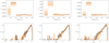 |
Fig. 2. Model fits to mock datasets used as tests. Top row: black lines show the true value of the birthrate αi parameters. The orange lines show the estimated αi parameters for three different realisations of the mock datasets generated from the same initial parameters. The orange shaded areas correspond to the 1- and 2-σ levels. Bottom row: black histograms represent the magnitude distribution of three different mock datasets. The thick orange histograms represent the magnitude distribution obtained by using the best fit αi. The dashed histograms represent the magnitude distribution obtained by using the 16th and 84th percentiles for αi. |
4. Results
In this section, we present the results obtained by fitting our model to the data presented in Sect. 2. We computed the values and uncertainties for the coefficients αi, j that imply b(τi | xj, αj) for all the spaxels xj in the map of Fig. 1 (right) by sampling the likelihood of Eq. (9). Example values of the αi parameters and their uncertainties are given in Table 1 and are available on CDS.
Selected values and uncertainties for three spaxels, and corresponding coordinates.
These results are essentially number- or mass-density maps of mono-age stellar populations (in five age bins) across our surrounding 6 kpc × 6 kpc area of the Galactic disc (Figs. 3 and 4), as well as the overall radial gradients they show (Figs. 5 and 6). When summing over the entire area, we obtain an estimate of the integrated age distribution of the stars (Fig. 7), which reflects the formation rate of the stars that are now in this portion of the disc.
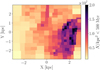 |
Fig. 3. Density distribution of stars younger than 500 Myr in the Galacic plane, as derived from Eq. (11), i.e. by using the best estimates for the birthrate coefficients, αi, in each spaxel, j. |
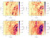 |
Fig. 4. Density distribution of stars with ages of 5 < t < 50 Myr (top left), 50 < t < 100 Myr (top right), 100 < t < 200 Myr (bottom left), and 200 < t < 500 Myr (bottom right). The density distribution changes as a function of time, becoming gradually smoother. Over-arching structures corresponding to spiral arms are visible for all age intervals. The solid black lines indicate the location of the spiral arms from Reid et al. (2019). |
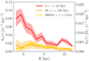 |
Fig. 5. Distribution of star formation rate surface density as a function of galactocentric radius. The thick lines correspond to the average star formation rate surface density for different age intervals (red: 5 < τ < 10 Myr; orange: 50 < τ < 100 Myr; yellow: 400 < Myrτ < 1 Gyr). The shaded areas correspond to the 16th and 84th percentiles. The left Y-axis shows the star formation rate expressed as the total number of stars born; the right Y-axis shows the more conventional amount of stellar mass formed, which requires the adoption of an IMF (here, Kroupa 2001). |
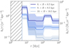 |
Fig. 6. Star formation rate density in different galactocentric radii, as a function of time. The left and right Y-axes show the SFR expressed as the total number of stars born and as the stellar mass formed, respectively. The thick lines correspond to the average star formation rate surface density for three intervals in galactocentric radius. The shades areas correspond to the 16th and 84th percentiles. Ages below 5 Myr are not included in our analysis, and thus the corresponding area in the plot is hatched. |
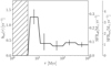 |
Fig. 7. Effective star formation history of the sample, in units of yr−1 (left y-axis) and M⊙ yr−1 (first right y-axis). The second right y-axis corresponds to the total SFR obtained by multiplying by the ratio f = SFR5 − 11/SFRtot (see Sect. 5). Vertical bars correspond to errors on the parameters. Ages below 5 Myr are not included in our analysis, and thus the corresponding area in the plot is hatched. |
4.1. Mono-age stellar density maps of the Galactic disc
Figure 3 shows the number surface density of stars, n(Δτ | x, α), younger than 500 Myr, defined as
 (11)
(11)
where the integral of b(τ | x, αbest) over time gives the number of stars formed between τmin < τ < τmax and Area(x) is the spaxel area in kpc2. The density distribution in the Galactic plane of sources younger than 500 Myr is qualitatively very similar to that shown in Fig. 1, lending credence to our results. The total number of stars in each spaxel is different from the number of observed stars per spaxel, because with Eq. (11) we predict the total number of stars at all masses, not only those included in the filtered sample from Z21. These maps can be converted into maps of the (hypothetical, initial) stellar surface mass density of stars in that age bin, simply by multiplying by the initial mean mass per star, ⟨M*⟩ = 0.22 M⊙ for our Kroupa IMF.
The density distribution of the sample can be further investigated by splitting the stars into age bins, with ages of 5 < τ < 50 Myr (Fig. 4, top left), 50 < τ < 100 Myr (Fig. 4, top right), 100 < τ < 200 Myr (Fig. 4, bottom left), and 200 < τ < 500 Myr (Fig. 4, bottom right). The appearance of these maps changes as a function of age. In the youngest age interval (5 < τ < 50 Myr), the density distribution traces massive star-forming regions, which are visible as prominent overdense clumps in Figs. 1 and 3 (see also Zari et al. 2021; Poggio et al. 2021). The distributions of stars in the less young age intervals appear smoother and do not show dense clumps, certainly not beyond the age of one dynamical timescale or galactocentric rotation: ∼200 Myr. However, arch-like or spiral structures are visible for all age groups. The strength of spiral arms is quantified in Fig. A.1.
4.2. Radial trends of the young star density
For potential comparison with in particular external galaxies (González Delgado et al. 2016), we now look at the dependence of the young star density on galactocentric radius RGC, averaging over the azimuthal angle that lies inside our 6 kpc × 6 kpc box, simply summing over all spaxels in a certain RGC range:
 (12)
(12)
where S is the total area of these spaxels.
Figure 5 shows the radial distribution of nR(τi | RGC) for three different age intervals τi: 5 < τ < 10 Myr, 50 < τ < 100 Myr, and 400 Myr < τ < 1 Gyr. While the older age bins only show a shallow gradient, the radial density gradient among stars τ < 10 Myr is quite steep, and shows a prominent peak at R ∼ 6 kpc and hints of two peaks at R ∼ 8 kpc and R ∼ 10 kpc.
Figure 6 shows the azimuthally averaged mean birthrate parameter nR(τi|R) for different galactocentric radii. The different galactocentric annuli do not only vary significantly in their normalisation, but also their relative age distributions. While all show a distinct increase at the youngest ages, this increase is fractionally largest well outside the solar radius. The age distribution well inside the solar radius may have had a second peak between 100 and 300 Myr ago (which may be dominated by the contributions along the galactocentric angle ϕ = −0.115; see Fig. A.1).
4.3. Effective overall star formation rate
As the final step in the presentation of our results, we show the age distribution when summed over the entire 6 × 6 kpc2 area. We define the total ‘effective’ birthrate btot as
 (13)
(13)
by summing over all the j spaxels in the map (and not normalising by the area). Below we discuss to what extent this age distribution reflects the overall star formation rate across the Galactic disc.
Units of btot(τ) are of stars/year, which we converted to the more conventional M⊙ yr−1 by multiplying by the mean stellar mass derived from our assumed IMF ⟨M⟩ = 0.22 M⊙. This is shown in Fig. 7, along with btot(τ) on the left Y-axis and SFReff on the first right Y-axis. Both values refer to the entire 6 × 6 kpc2 area, a much larger area than previous quantitative studies for this age range, but of course not the ‘entire disc’.
Figure 7 shows that the age distribution of stars is approximately uniform between 20 Myr and 1 Gyr at 0.4 yr−1 (or 0.08 M⊙ year−1. Remarkably, the effective star formation rate seems to have been three times higher in the last ∼10 − 20 Myr. It appears that the Galactic disc, or at least the large patch we consider here, has just lit up in young stars.
5. Discussion and summary
In the previous sections, we estimate the recent star formation history of the extended solar neighbourhood and found that it has recently increased by a factor of ∼3. We now estimate the global star formation rate of the Galactic disc and put this result into context by comparing with previous literature studies. We then use simulations to quantify to what extent global conclusions can be extrapolated from local measurements.
5.1. Comparison to existing work
Assuming that the fraction of the disc that we are probing is representative of the entire Milky Way (see Sect. 5.2), we can derive the ‘total’ SFR of the Milky Way. To do so, we considered the youngest bin, τ ≲ 10 Myr, as the best approximation to the ‘current SFR’, and we extended SFReff, 5 − 10 Myr to the disc. Since the surface density of star formation decreases strongly as a function of radius, we presume that the star formation rate surface density is described well by an exponential radial profile (Eq. (14)) within 4.5–15 kpc, with a scale length of L = 3.5 kpc (Zari et al. 2021, see Appendix B.2):
 (14)
(14)
We chose Rmin = 4.5 kpc and Rmax = 15 kpc following Reed (2005) and Davies et al. (2011) and thus excluded the central region of the Galaxy. In the radial range covered by our data, ∼5 and ∼11 kpc from the Galactic centre, the total SFR is
 (15)
(15)
where Δϕ ≈ 0.7 rad corresponds to the range of azimuth angles covered. The ratio f = SFR5 − 11/SFRtot ≈ 8% reflects the fraction of the MW disc considered in this study. We thus find that the total SFR of the Milky Way implied by this model is  (see Fig. 7).
Recent analogous estimates of the star formation rate of the Milky Way are between 1.65 ± 0.19 M⊙ yr−1 (Licquia & Newman 2015) and 1.9 ± 0.4 M⊙ yr−1 (Chomiuk & Povich 2011), similar to but lower than the value we find. Reasons for this discrepancy may reflect differences in the assumed IMF, the spatial coverage, and the age of the tracers used; these are discussed below.
In their Sect. 3, Chomiuk & Povich (2011) reviewed the different methods used to estimate the Milky Way SFR. Such methods rely on Lyman continuum photon rates (e.g., Mezger 1978; Smith et al. 1978; McKee & Williams 1997; Murray & Rahman 2010), infrared emission and YSO counts (Robitaille & Whitney 2010; Davies et al. 2011), or massive star counts and supernova rates (Reed 2005; Diehl et al. 2006). In their study, Chomiuk & Povich (2011; and thus also Licquia & Newman 2015) normalised previous results to the same IMF, adopting the IMF from Kroupa & Weidner (2003, KW03) as a reference: ξ(m)∝m−Γ with Γ = 1.3 for masses between 0.1 and 0.5 M⊙ and Γ = 2.3 for masses between 0.5 and 100 M⊙. Since our sample is predominately composed of massive stars of which most will be in unresolved binary (or multiple) systems (see e.g., Sana et al. 2014), it seems appropriate to adopt an IMF that is explicitly corrected for unresolved binaries (Kroupa 2001, 2002) reported in Sect. 3. The choice of the IMF impacts, of course, the relation between the observed and modelled luminosity function n(MK|τ) and the implied ‘underlying’ total stellar mass (Eqs. (4) and (6)). In our formulation of the problem, this affects the inference of the birthrate parameter, αi, and the mean stellar mass that is used to convert the SFR to units of M⊙ yr−1, which for the KW03 IMF is ⟨M⟩ = 0.63 M⊙. To quantify the impact of the choice of IMF on our results, we re-ran the analysis using KW03 IMF. This yields an analogous estimate for the total SFR of 2.3 ± 0.4 M⊙ yr−1, which is consistent with the estimates of Chomiuk & Povich (2011) and slightly higher than those of Licquia & Newman (2015).
There are strong assumptions behind the space distribution of different tracers used to study the global SFR or the Milky Way (including ours, see Sect. 5.2). For instance, the distance to HII regions are biased against distant sources, and studies that employ HII emission to compute the Galactic SFR usually account for this by doubling the luminosity of sources in our half of the Galaxy (Mezger 1978; Smith et al. 1978; McKee & Williams 1997; Murray & Rahman 2010). In other cases, distances are not available; for example, the space distribution of YSOs assumed by Robitaille & Whitney (2010; see their Fig. 2) is quite different than what we used in this work, which is instead more similar to what was proposed by Reed (2005) and Davies et al. (2011).
Finally, the lifetimes of the tracers used in other studies are different. The estimate (0.68 − 1.45 M⊙ yr−1) of Robitaille & Whitney (2010) assumed a YSO lifetime of ≈2 Myr, which is younger than the minimum age considered here (5 Myr). Murray & Rahman (2010) used a lifetime for HII regions of 3.7 Myr following McKee & Williams (1997), which is slightly longer than the 3 Myr used by Mezger (1978), and again younger than our minimum age. Reed (2005) assigned lifetimes from ≈3.5 Myr to ≈20 Myr based on the luminosities of his sample of O- and B-type stars. We note that our estimate of the global effective star formation rate is already 3× lower for stars that are 20–50 Myr old.
The recent increase in effective SFR that we find is qualitatively similar to that found by Ruiz-Lara et al. (2020). Ruiz-Lara et al. (2020) modelled Gaia DR2 observed colour–magnitude diagrams to infer the star formation history within 2 kpc around the Sun and found three star formation enhancements that occurred ∼5.7, 1.9, and 1.0 Gyr ago and a hint of a fourth possible star formation burst spanning the last 70 Myr. Ruiz-Lara et al. (2020) did not express their results in M⊙ yr−1, complicating a direct comparison. They proposed that such enhancements are due to recurrent interactions between the Milky Way and the Sagittarius dwarf galaxy (Ibata et al. 1994; Laporte et al. 2018). We confirm the recent enhancement in star formation activity of the Galactic disc with a higher level of confidence and we constrain it to the last 10 Myr. Given that we find distinct temporal variations in the Galaxy’s effective star formation rate over the last 100 Myr (Fig. 7), matching the exact age distribution of the tracers would be crucial for a more quantitative comparison with Cignoni et al. (2006) and Ruiz-Lara et al. (2020).
Figure 4 shows that the location of the density enhancements broadly coincides between the youngest and older stellar age intervals. This suggests that the spiral pattern is associated not only with young star-forming regions but also with the underlying mass density (Eskridge et al. 2002; Binney & Tremaine 2008), at least for τ < 500 Myr. Consequently, Fig. 4 represents evidence that those spiral arms that show up in all our mono-age maps are indeed stellar-mass overdensities. Spiral arms that are seen in stellar populations of different ages are also observed in external galaxies. For instance, Meidt et al. (2021) compared the distribution of molecular gas (tracing star formation) and 3.6 μm emission (tracing old disc populations) across 67 star-forming galaxies with different morphological properties, often finding coincidence. However, not all spiral arms in the Milky Way disc, inferred from masers, for example, are reflected in stellar-mass overdensities in our maps among stars with τ ≲ 0.5 Gyr (see top left panel of Fig. 4).
5.2. How closely does the best-fit age distribution reflect the overall disc SFR?
The area sampled by our OBA sample is only ≈8% of the entire Galactic disc. Large-scale spatial variations in the star formation rate density or stellar ages, such as large-scale spiral arms, could bias the generalisation from this sample to the entire Galactic disc. To test how much variance could be expected, we examine the final snapshot of cosmological simulations of Milky Way-like galaxies. We used the TNG50 cosmological simulation (Pillepich et al. 2019; Nelson et al. 2019), whose numerical resolution reaches that of zoomed-in simulations (reaching a baryonic mass of 8.5 × 10⁴ M⊙). IN TNG50, we selected Milky Way-like galaxies based on their stellar mass, discyness, and morphology. Specifically, we require the following:
-
1010.5 ≤ M⋆/M⊙ ≤ 1011.2
-
over 40% of stars on near-circular orbits (with circularities ≥0.7, Genel et al. 2015)
-
a central bar
-
a non-zero star formation rate at z = 0,
leading to N = 78 galaxies. We centred and align a Cartesian coordinate system with the vertical axis aligned with the angular momentum of the disc. To mimic our observed sample, we placed a solar neighbourhood at (R, z, φ) = (8, 0, φ) and selected stars in a cylinder centred on the Sun with a 3 kpc radius. To investigate how the location φ of the Sun influences the results, we varied the azimuth of the Sun and measured the local star formation history (from the local age distribution), thereby estimating the amplitude biases in local datasets.
Sampling all galaxies and all azimuthal angles for the position of the hypothetical sun, we derived the distribution of

where the denominator is the number of stars per age interval in the patch, and the denominator is the same quantity in the entire annulus. We find that azimuthal variations of the recent ‘effective’ SFR in a patch of R = 3 kpc reflect the global average typically within factor of ∼1.5. These variations are shown in Fig. 8 as orange bands, reflecting the conceptual uncertainties of extrapolating the age distribution measured within our volume to a global star formation rate of the Galactic disc. This figure shows that these uncertainties are considerable. Nonetheless, the increase in the frequency of very young stars we find reflects a global recent increase in the Galaxy SFR. While it is unlikely that the Sun has just moved into a patch of higher star formation activity, it is not obvious that there are plausible physical mechanisms that would boost the Milky Way’s global star formation rate on timescales shorter than ∼20 Myr. Our comparison with simulations implies that an SFR increase in our observed volume likely reflects a global SFR increase; however, we need to be open to the possibility that our SFR estimates for the youngest age bin reflect a localised SFR fluctuation with much more modest global SFR changes across the whole Milky Way.
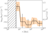 |
Fig. 8. Logarithm of the effective star formation history of the sample shown in Fig. 7. The orange bands show the expected azimuthal variations of the effective star formation history as derived by analysing Milky Way analogues in TNG50. |
5.3. Summary
In this study, we modelled the observed K-band absolute magnitude distribution MK of the sample of massive young stars presented in Zari et al. (2021) to infer the age distribution of stars within ∼3 kpc from the Sun and the effective star formation rate (SFR) of the Milky Way. We divided our volume into spaxels of different sizes and assumed that in each spaxel the MK distribution depended only on the birthrate. We parametrised the birthrate with a step function with five age intervals to avoid imposing a particularly restrictive functional form, and we derived the parameters characterising the birthrate by comparing our predicted magnitude distribution with the data magnitude distribution by quantifying the likelihood of the data.
We derived the density distribution of stars of different ages in the Galactic plane. We found that stars with ages of < 50 Myr are clustered in compact groups that trace Galactic spiral arms. Over-densities corresponding to spiral arms are, however, also visible in the density distribution of older populations. We derived the star formation history of our sample over the last Gyr by estimating the effective birthrates (i.e., the birthrate that would lead to the observed magnitude distribution) for all the spaxels in our volume, and adding them over all the spaxels.
We found that the age distribution (or total birthrate) is almost uniform between 20 Myr and 1 Gyr, but has increased by almost a factor or 3 in the last ∼10–20 Myr. By using TNG50 simulations of Milky Way analogue galaxies, we derived that azimuthal SFR variations are considerable but smaller than the recent SFR increase. It is not clear which physical mechanisms could be responsible for this increase; hence, we cannot exclude the possibility that it might reflect a local fluctuation, due to the large number of massive star-forming regions within our volume. Based on the assumption that the local value could be extended to the entire Milky Way disc, we estimated the current (last ∼10 Myr) SFR of the entire Milky Way disc to be  .
.
A model for which we do not assume a specific functional form, but have parameters for.
Acknowledgments
We thank the referee for their comments that improved the clarity of the manuscript. We are also grateful to D. Weinberg for valuable input. NF was supported by the Natural Sciences and Engineering Research Council of Canada (NSERC), [funding reference number CITA 490888-16] through the CITA postdoctoral fellowship and acknowledges partial support from a Arts & Sciences Postdoctoral Fellowship at the University of Toronto. This work has made use of data from the European Space Agency (ESA) mission Gaia (https://www.cosmos.esa.int/gaia), processed by the Gaia Data Processing and Analysis Consortium (DPAC, https://www.cosmos.esa.int/web/gaia/dpac/consortium). Funding for the DPAC has been provided by national institutions, in particular the institutions participating in the Gaia Multilateral Agreement. This publication makes use of data products from the Two Micron All Sky Survey, which is a joint project of the University of Massachusetts and the Infrared Processing and Analysis Center/California Institute of Technology, funded by the National Aeronautics and Space Administration and the National Science Foundation. This research made use of Astropy, (Astropy Collaboration 2013, 2018), matplotlib (Hunter 2007), numpy (Harris et al. 2020), scipy (Virtanen et al. 2020). This work would not have been possible without the countless hours put in by members of the open-source community all over the world.
References
- Astropy Collaboration (Robitaille, T. P., et al.) 2013, A&A, 558, A33 [NASA ADS] [CrossRef] [EDP Sciences] [Google Scholar]
- Astropy Collaboration (Price-Whelan, A. M., et al.) 2018, AJ, 156, 123 [Google Scholar]
- Binney, J., & Tremaine, S. 2008, Galactic Dynamics, 2nd edn. (Princeton: Princeton University Press) [Google Scholar]
- Bouwens, R. J., Illingworth, G. D., Oesch, P. A., et al. 2011, ApJ, 737, 90 [NASA ADS] [CrossRef] [Google Scholar]
- Bovy, J., Rix, H.-W., Liu, C., et al. 2012, ApJ, 753, 148 [Google Scholar]
- Bressan, A., Marigo, P., Girardi, L., et al. 2012, MNRAS, 427, 127 [NASA ADS] [CrossRef] [Google Scholar]
- Chen, Y., Bressan, A., Girardi, L., et al. 2015, MNRAS, 452, 1068 [Google Scholar]
- Chiappini, C., Matteucci, F., & Gratton, R. 1997, ApJ, 477, 765 [Google Scholar]
- Chomiuk, L., & Povich, M. S. 2011, AJ, 142, 197 [Google Scholar]
- Cignoni, M., Degl’Innocenti, S., Prada Moroni, P. G., & Shore, S. N. 2006, A&A, 459, 783 [NASA ADS] [CrossRef] [EDP Sciences] [Google Scholar]
- Davies, B., Hoare, M. G., Lumsden, S. L., et al. 2011, MNRAS, 416, 972 [Google Scholar]
- de Rossi, M. E., Tissera, P. B., De Lucia, G., & Kauffmann, G. 2009, MNRAS, 395, 210 [NASA ADS] [CrossRef] [Google Scholar]
- Diehl, R., Halloin, H., Kretschmer, K., et al. 2006, Nature, 439, 45 [CrossRef] [PubMed] [Google Scholar]
- Eskridge, P. B., Frogel, J. A., Pogge, R. W., et al. 2002, ApJS, 143, 73 [NASA ADS] [CrossRef] [Google Scholar]
- Foreman-Mackey, D., Hogg, D. W., Lang, D., & Goodman, J. 2013, PASP, 125, 306 [Google Scholar]
- Genel, S., Fall, S. M., Hernquist, L., et al. 2015, ApJ, 804, L40 [NASA ADS] [CrossRef] [Google Scholar]
- González Delgado, R. M., Cid Fernandes, R., Pérez, E., et al. 2016, A&A, 590, A44 [NASA ADS] [CrossRef] [EDP Sciences] [Google Scholar]
- Harris, C. R., Millman, K. J., van der Walt, S. J., et al. 2020, Nature, 585, 357 [NASA ADS] [CrossRef] [Google Scholar]
- Hunter, J. D. 2007, Comput. Sci. Eng., 9, 90 [NASA ADS] [CrossRef] [Google Scholar]
- Ibata, R. A., Gilmore, G., & Irwin, M. J. 1994, Nature, 370, 194 [Google Scholar]
- Kauffmann, G., & Haehnelt, M. 2000, MNRAS, 311, 576 [Google Scholar]
- Kennicutt, R. C., & Evans, N. J. 2012, ARA&A, 50, 531 [NASA ADS] [CrossRef] [Google Scholar]
- Kreckel, K., Faesi, C., Kruijssen, J. M. D., et al. 2018, ApJ, 863, L21 [NASA ADS] [CrossRef] [Google Scholar]
- Kroupa, P. 2001, MNRAS, 322, 231 [NASA ADS] [CrossRef] [Google Scholar]
- Kroupa, P. 2002, Science, 295, 82 [Google Scholar]
- Kroupa, P., & Weidner, C. 2003, ApJ, 598, 1076 [NASA ADS] [CrossRef] [Google Scholar]
- Lada, C. J., Lombardi, M., & Alves, J. F. 2010, ApJ, 724, 687 [Google Scholar]
- Laporte, C. F. P., Johnston, K. V., Gómez, F. A., Garavito-Camargo, N., & Besla, G. 2018, MNRAS, 481, 286 [Google Scholar]
- Licquia, T. C., & Newman, J. A. 2015, ApJ, 806, 96 [NASA ADS] [CrossRef] [Google Scholar]
- Madau, P., Ferguson, H. C., Dickinson, M. E., et al. 1996, MNRAS, 283, 1388 [Google Scholar]
- McKee, C. F., & Williams, J. P. 1997, ApJ, 476, 144 [CrossRef] [Google Scholar]
- Meidt, S. E., Leroy, A. K., Querejeta, M., et al. 2021, ApJ, 913, 113 [NASA ADS] [CrossRef] [Google Scholar]
- Mezger, P. O. 1978, A&A, 70, 565 [NASA ADS] [Google Scholar]
- Moe, M., & Di Stefano, R. 2017, ApJS, 230, 15 [Google Scholar]
- Murray, N., & Rahman, M. 2010, ApJ, 709, 424 [NASA ADS] [CrossRef] [Google Scholar]
- Nelson, D., Springel, V., Pillepich, A., et al. 2019, Comput. Astrophys. Cosmol., 6, 2 [Google Scholar]
- Pillepich, A., Nelson, D., Springel, V., et al. 2019, MNRAS, 490, 3196 [Google Scholar]
- Poggio, E., Drimmel, R., Cantat-Gaudin, T., et al. 2021, A&A, 651, A104 [NASA ADS] [CrossRef] [EDP Sciences] [Google Scholar]
- Reed, B. C. 2005, AJ, 130, 1652 [NASA ADS] [CrossRef] [Google Scholar]
- Reid, M. J., Menten, K. M., Brunthaler, A., et al. 2019, ApJ, 885, 131 [Google Scholar]
- Rix, H.-W., & Bovy, J. 2013, A&A Rev., 21, 61 [NASA ADS] [CrossRef] [Google Scholar]
- Rix, H.-W., Hogg, D. W., Boubert, D., et al. 2021, AJ, 162, 142 [NASA ADS] [CrossRef] [Google Scholar]
- Robitaille, T. P., & Whitney, B. A. 2010, ApJ, 710, L11 [CrossRef] [Google Scholar]
- Robitaille, T. P., Meade, M. R., Babler, B. L., et al. 2008, AJ, 136, 2413 [NASA ADS] [CrossRef] [Google Scholar]
- Ruiz-Lara, T., Gallart, C., Bernard, E. J., & Cassisi, S. 2020, Nat. Astron., 4, 965 [NASA ADS] [CrossRef] [Google Scholar]
- Rybizki, J., Green, G. M., Rix, H.-W., et al. 2022, MNRAS, 510, 2597 [NASA ADS] [CrossRef] [Google Scholar]
- Sana, H., Le Bouquin, J. B., Lacour, S., et al. 2014, ApJS, 215, 15 [Google Scholar]
- Smith, L. F., Biermann, P., & Mezger, P. G. 1978, A&A, 66, 65 [NASA ADS] [Google Scholar]
- Tang, J., Bressan, A., Rosenfield, P., et al. 2014, MNRAS, 445, 4287 [NASA ADS] [CrossRef] [Google Scholar]
- Virtanen, P., Gommers, R., Oliphant, T. E., et al. 2020, Nat. Methods, 17, 261 [Google Scholar]
- Williams, B. F., Dalcanton, J. J., Johnson, L. C., et al. 2011, ApJ, 734, L22 [NASA ADS] [CrossRef] [Google Scholar]
- Zari, E., Rix, H. W., Frankel, N., et al. 2021, A&A, 650, A112 [NASA ADS] [CrossRef] [EDP Sciences] [Google Scholar]
Appendix A: Azimuthal birthrate variations
To quantify the birthrate spatial variations, we considered five azimuths and studied the variations of bbest(τ|x, α) as a function of galactocentric radius for the same age intervals as in Fig. 5. Figure A.1 shows that the sharp peaks in birthrate for 5 < τ < 10 Myr coincide with the locations of spiral arm segments, while for the older age ranges the birthrate is lower and does not correlate strongly with the position of spiral arms.
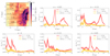 |
Fig. A.1. Birthrates as a function of galactocentric radius and azimuths. Top left: Same as Fig. 3, the dashed lines correspond to the different azimuths considered. Top centre, right, and bottom: Birthrate as a function of galactocentric radius for three different age intervals at five different azimuths (as indicated in the panels). The colour scheme is the same as in Fig. 5. The thick lines correspond to the average birthrate, and the shaded areas correspond to the 16th and 84th percentiles. |
All Tables
Selected values and uncertainties for three spaxels, and corresponding coordinates.
All Figures
|
Fig. 1. Density distribution of the filtered sample of massive hot stars from Zari et al. (2021). In the left panel, the coloured lines represent the spiral arm locations derived by Reid et al. (2019). The right panel highlights the 6 × 6 kpc region considered in this study. Such region is divided in ‘spaxels’ of different sizes, each containing the same number of sources. In both panels, the Sun is in X, Y = (0, 0). |
| In the text | |
|
Fig. 2. Model fits to mock datasets used as tests. Top row: black lines show the true value of the birthrate αi parameters. The orange lines show the estimated αi parameters for three different realisations of the mock datasets generated from the same initial parameters. The orange shaded areas correspond to the 1- and 2-σ levels. Bottom row: black histograms represent the magnitude distribution of three different mock datasets. The thick orange histograms represent the magnitude distribution obtained by using the best fit αi. The dashed histograms represent the magnitude distribution obtained by using the 16th and 84th percentiles for αi. |
| In the text | |
|
Fig. 3. Density distribution of stars younger than 500 Myr in the Galacic plane, as derived from Eq. (11), i.e. by using the best estimates for the birthrate coefficients, αi, in each spaxel, j. |
| In the text | |
|
Fig. 4. Density distribution of stars with ages of 5 < t < 50 Myr (top left), 50 < t < 100 Myr (top right), 100 < t < 200 Myr (bottom left), and 200 < t < 500 Myr (bottom right). The density distribution changes as a function of time, becoming gradually smoother. Over-arching structures corresponding to spiral arms are visible for all age intervals. The solid black lines indicate the location of the spiral arms from Reid et al. (2019). |
| In the text | |
|
Fig. 5. Distribution of star formation rate surface density as a function of galactocentric radius. The thick lines correspond to the average star formation rate surface density for different age intervals (red: 5 < τ < 10 Myr; orange: 50 < τ < 100 Myr; yellow: 400 < Myrτ < 1 Gyr). The shaded areas correspond to the 16th and 84th percentiles. The left Y-axis shows the star formation rate expressed as the total number of stars born; the right Y-axis shows the more conventional amount of stellar mass formed, which requires the adoption of an IMF (here, Kroupa 2001). |
| In the text | |
|
Fig. 6. Star formation rate density in different galactocentric radii, as a function of time. The left and right Y-axes show the SFR expressed as the total number of stars born and as the stellar mass formed, respectively. The thick lines correspond to the average star formation rate surface density for three intervals in galactocentric radius. The shades areas correspond to the 16th and 84th percentiles. Ages below 5 Myr are not included in our analysis, and thus the corresponding area in the plot is hatched. |
| In the text | |
|
Fig. 7. Effective star formation history of the sample, in units of yr−1 (left y-axis) and M⊙ yr−1 (first right y-axis). The second right y-axis corresponds to the total SFR obtained by multiplying by the ratio f = SFR5 − 11/SFRtot (see Sect. 5). Vertical bars correspond to errors on the parameters. Ages below 5 Myr are not included in our analysis, and thus the corresponding area in the plot is hatched. |
| In the text | |
|
Fig. 8. Logarithm of the effective star formation history of the sample shown in Fig. 7. The orange bands show the expected azimuthal variations of the effective star formation history as derived by analysing Milky Way analogues in TNG50. |
| In the text | |
|
Fig. A.1. Birthrates as a function of galactocentric radius and azimuths. Top left: Same as Fig. 3, the dashed lines correspond to the different azimuths considered. Top centre, right, and bottom: Birthrate as a function of galactocentric radius for three different age intervals at five different azimuths (as indicated in the panels). The colour scheme is the same as in Fig. 5. The thick lines correspond to the average birthrate, and the shaded areas correspond to the 16th and 84th percentiles. |
| In the text | |
Current usage metrics show cumulative count of Article Views (full-text article views including HTML views, PDF and ePub downloads, according to the available data) and Abstracts Views on Vision4Press platform.
Data correspond to usage on the plateform after 2015. The current usage metrics is available 48-96 hours after online publication and is updated daily on week days.
Initial download of the metrics may take a while.