| Issue |
A&A
Volume 669, January 2023
|
|
|---|---|---|
| Article Number | A100 | |
| Number of page(s) | 11 | |
| Section | Interstellar and circumstellar matter | |
| DOI | https://doi.org/10.1051/0004-6361/202040244 | |
| Published online | 18 January 2023 | |
Global kinematics study of OH masers in W49N
1
Instituto Nacional de Astrofísica, Óptica y Electrónica,
C. Luis Enrique Erro No. 1,
Tonantzintla,
Pue. CP 72840, Mexico
e-mail: This email address is being protected from spambots. You need JavaScript enabled to view it.
; This email address is being protected from spambots. You need JavaScript enabled to view it.
2
Instituto de Geofísica y Astronomía,
Street 212, No. 2906, between 29 and 31.
CP 11600,
La Coronela, La Lisa, La Habana, Cuba
e-mail: This email address is being protected from spambots. You need JavaScript enabled to view it.
Received:
25
December
2020
Accepted:
30
September
2022
Abstract
Context. Star formation is underway in the W49N molecular cloud (MC) at a high level of efficiency, with almost twenty ultra-compact (UC) HII regions observed thus far, indicating a recent formation of massive stars. Previous works have suggested that this cloud is undergoing a global contraction.
Aims. We analyse the data on OH masers in the molecular cloud W49N, observed with the VLBA at the 1612, 1665, and 1667 MHz transitions in left circular polarization (LCP) and right circular polarization (RCP) with an aim to study the global kinematics of the masers.
Methods. We carried out our study based on the locations and observed velocities of the maser spots, Vobs. We found the location (α, δ)m of the maximum correlation between V = Vobs−Vsys (with Vsys the systemic velocity) and distance to it. The velocities were fitted to the straight line of Vobs−Vsys versus d(α,δ)m, resulting in Vftd. The difference between the fitted values and those obtained from observations is ∆ V = (Vobs−Vsys)-Vftd. The Vobs−Vsys velocity shows a gradient as a function of the distance to (α, δ)m, where the closer spots have the largest velocities. Spots with similar velocities are located in different sectors, with respect to (α, δ)m. Then, we assumed that the spots are moving towards a contraction centre (CCOH), which is at the apex of a CONUS. We also assumed that the distance of each spot to CCOH is dcc = √2 d(α,δ)m and that they fall with a velocity Vcc = √2Vftd, with the total velocity being VTot = Vcc + √2 Δ V. Using this velocity, we estimated the free-fall velocity.
Results. The coordinates of (α, δ)m are effectively (α2000 = 19:10:13.1253, δ2000 = 9:6:13.570). The observed dispersion with respect to the global trend against dcc, shows a maximum at 0.12 pc, with a decay from 0.12 to 0.19 pc, which is faster than that taking place between 0.19 and 0.42 pc. Based on VTot, an inner mass of Minn = 2500 M⊙ was estimated. In addition, the estimated accretion rate is Ṁ = 1.4×10⁻³ M⊙yr−1, which requires a time of tinn = 1.8×10⁶ yr to accumulate Minn. The free-fall time, assuming n = 1×10⁻⁴ cm−3, is tff = 3.4×10⁵ yr. Performing the same procedure with published data that are of lower spatial resolution (than the VLBA data) produces similar results. For example, based on the available data, we find that (α, δ)m = (19:10:13.1392, 9:6:13.4387) J2000, which is at ≲ 0.3 asec from what has been calculated with the VLBA data, with an estimated inner mass of 2700 M⊙. A sub-collapse appears to be taking place in the region traced by the OH maser spots. Based on methanol maser cloudlets data, which lie in a smaller region, another possible centre of contraction is identified, which could be due to a sub-collapse towards a 75 M⊙ inner mass.
Conclusions. The velocities of the OH spots at W49N, along with their positions with respect to (α, δ)m, make it possible to trace a global kinematics that is apparently due to a sub-collapse in the W49N MC.
Key words: masers / ISM: clouds / ISM: kinematics and dynamics
© The Authors 2023
 Open Access article, published by EDP Sciences, under the terms of the Creative Commons Attribution License (https://creativecommons.org/licenses/by/4.0), which permits unrestricted use, distribution, and reproduction in any medium, provided the original work is properly cited.
This article is published in open access under the Subscribe-to-Open model. This email address is being protected from spambots. You need JavaScript enabled to view it. to support open access publication.
1 Introduction
The W49N molecular cloud (MC) is part of the W49A giant molecular cloud, located at a distance of 11.1 kpc (Zhang et al. 2013). The radial velocity of W49N has been estimated to be approximately 8.0 km s−1 (Welch et al. 1987). In this region, about 20 HII regions have been observed (Dreher et al. 1984; De Pree et al. 2000, 2004) in different spectral lines (De Pree et al. 1997; Kulczak-Jastrzebska 2017) and in the radio continuum (Wilner et al. 2001; Galván-Madrid et al. 2013). The HII regions, identified by Dreher et al. (1984) as ultra-compact (UC), are thought to be driven by O stars (Wilner et al. 2001), making this region one of the sites at our Galaxy characterised by the active formation of massive stars, with some of them estimated to be M* ≃ 25−35 M⊙ and even M* ≃ 45 M⊙ (Smith et al. 2009).
Masers of OH (Johnston & Hansen 1982; Kent & Mutel 1982; Argon et al. 2000) and of H2O (Gwinn et al. 1989, 1992; Gwinn 1994; Takefuji et al. 2016) have been observed in W49N. The OH spots detected by Kent & Mutel (1982) with the VLBI have velocities ranging from 4.6 to 21.1 km s−1 and Argon et al. (2000) those registered with the VLA, OH spots have velocities between 8 and 22 km s−1. The spots with more red-shifted velocities are mainly located at the west (W), while the less red-shifted appear at the east (E). H2O maser spots observed by Gwinn et al. (1992) at W49N, have been interpreted as arising at a bipolar outflow of a newly formed star. The spot velocity increases with distance, to a common centre of the flows (denoted by a square in Fig. 1), up to velocities greater than 200 km s−1 (Gwinn et al. 1992; Gwinn 1994). Each outflow extends about 1 arcsec from their common centre, denoted by a square in Fig. 1.
At other sources, the proper motions of OH maser spots have allowed for the local kinematics to be established as likely being due to the expansion of HII regions (Bloemhof et al. 1992; Fish & Reid 2007; Liu et al. 2015), as well as jets (Argon et al. 2003), outflows (Fish et al. 2011), and shells and rings (De Pree et al. 2000).
In W49N, a velocity gradient has been identified, based on a set of HII regions that form a ring (Welch et al. 1987) and it has been suggested that the cloud is in contraction. On the other hand, Serabyn et al. (1993) suggested that the kinematics is due to the collision of two molecular clouds. Rudolph et al. (1990) found inverted P-Cygni profiles in the HCO+ molecule in W51, which is an association of almost a dozen ultra-compact HII (UC-HII) regions and estimated that it is engaged in a global collapse. They get a mass accretion rate of  and an inner mass of 105 M⊙.
Methanol masers have been seen at W49N (Bartkiewicz et al. 2014; Pandian et al. 2011). They are found to be associated with high-mass star formation (e.g. Sanna et al. 2010a; Moscadelli et al. 2011) and are capable of tracing the kinematics close to the young stellar object (YSO, Moscadelli et al. 2011). At G16.59−0.05, methanol maser cloudlets trace a rotation around a central mass of about 35 solar mass (Sanna et al. 2010a).
A velocity gradient of each methanol maser cloudlet, Vgrad, has been seen in a number of sources. Here, the gradient at the cloudlets is compared with the velocity gradient seen at the radial velocity of the cloudlets. From multi-epoch observations, it is found that the velocity gradients and the proper motion vectors point in the same direction in the sky (Moscadelli et al. 2011).
There are still unsolved problems related to the formation of high-mass stars (see Motte et al. 2018; Zinnecker & Yorke 2007). For example, to explain how they can grow to high masses, even under the action of radiation feedback, and how many of them can grow in a given region of a molecular cloud. The latter is known as mass segregation, in hierarchical substructures, the most massive protostellar objects are generally located in the centre of a cluster surrounded by objects of lower mass (Bonnell et al. 2003). One possibility for having many massive stars is that the cores are massive enough when the star formation process begins. The switch-offof the fragmentation process can allow for the conservation of massive cores, which could be due to a slow build-up supported by turbulence or thanks to the stabilisation of massive clusters for a magnetic field (see McKee & Tan 2002; Commerçon et al. 2011; Myers et al. 2013) Also, as suggested by Welch et al. (1985), the accretion on a global scale, lasting for long timescales, could lead to the accumulation of high masses.
The models applied by Welch et al. (1985) and Rudolph et al. (1990) to interpret the velocity field, as well as the observed masses, agree with the idea that the OB associations are formed by the dynamic collapse of large regions in molecular clouds. A better understanding of the kinematics of the MC W49N will help us to gain a better insight into the processes of star formation and, in particular, the formation of OB associations.
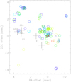 |
Fig. 1 Map of the OH maser spots respect the reference coordinates. The (0,0) location corresponds to α = 19:10:13.2091, δ = 09:06:12.485 (J2000). Respectively, the dark and light blue circles represent the 1667 MHz LCP and RCP maser spots; green and yellow is for 1665 MHz LCP and RCP; and orange and red circles for 1612 MHz LCP and RCP. The crosses indicate the locations of HII regions, reported by De Pree etal. (1997), with the corresponding letters used to refer to each of them. The square that overplots to the cross, which represents G1, corresponds to the location of the centre of the bipolar outflow of Gwinn et al. (1992). |
Number of spots recorded at each frequency and polarization.
2 Data analysis and results
The data were obtained in the OH lines at the following frequencies: 1667.35903, 1665.4018, and 1612.23101 MHz, hereafter referred to as 1667, 1665, and 1612 MHz, respectively. We are using the same data as Deshpande et al. (2013) with no new calibrations. The observations were made on 6 October 2005, with the Very Long Baseline Array (VLBA) interferometer. Left circular polarization (LCP) and right circular polarization (RCP) are observed simultaneously in about 240 spectral channels with a resolution of 0.1 km s−1 in a range of about 22 km s−1. The beam size is about 20 milliarcseconds (mas) by 15 mas at a position angle of 84 degrees. The reference coordinates are α = 19:10:13.2091 and δ = 09:06:12.485 (J2000).
To identify maser spots and estimate their flux, central velocity, and coordinates, Astronomical Image Processing System (AIPS) routines were used. In total, 205 spots were identified, in the three observation frequencies at the two polarizations (Table 1 and Fig. 1). The size of all the spots is greater than the interferometer beam, indicating that the spots are spatially resolved. The field of the OH spots is at the SW end of the Welch ring of HII regions, in a field made up of about 6 asec sides (Fig. 1). The observed velocity of the spots, Vobs, is taken respect to the systemic velocity of 8.0 km s−1 (Welch et al. 1987) and it spans about 18.6 km s−1. The spots with red-shifted Vobs are predominantly located in the W of the map, while the blue-shifted in the E, as reported by Kent & Mutel (1982). This is particularly clear for the frequencies where more spots are seen (1665 and 1667 MHz) at both polarizations (LCP and RCP).
The bipolar outflow lies on the HII region denoted as G1 by De Pree et al. (1997), as also found by Bloemhof (2000). The common centre of the outflows, traced by the H2O maser spots, becomes – at a location given by an offset in mas of (3110, 380) – relative to the VLBA reference coordinates.
In order to study the global kinematics of the OH spots, we tested the global velocity field to see if it shows a gradient. In spots separated by distances <1 asec, gradients are observed, however, we did not test single groups of spots, but all the spots across the whole field.
As mentioned above, the OH maser spots that are more red-shifted are in the east, while the less red-shifted ones are in the west. We searched for the possibility that the velocity of the spots versus the distance, with regard to a given location between the groups with different shifts, fits a straight line function. With this purpose, we applied the χ2 test. The χ2 error is the sum of squared differences between the values of Vobs−Vsys and those of Vftd, where these last values result from the fit for the distances, dij, of the spots to the location (αi, δj), in mass offsets respect the VLBA reference. The smaller the χ2 value, the better the fit.
We estimated χ2 for different locations (αi, δj), regularly separated in both, α and δ, thus forming a mesh. First, we used a mesh that encompasses the whole field of view (FOV) and for each point of the mesh, the test was applied. Based on these results, it is seen that, certainly, in the middle locations of the FOV, χ2 takes lower values than the rest locations of the FOV. Then, another mesh, with regularly spaced points by ∆α = 10 mas offsets in α and δ (i.e. with respect to the reference coordinates) and in the range, in mas offsets, from 5000 to −4000 in α and from −4500 to 4500 mas in δ is used to identify the minimum value of χ2 (Fig. 2). For each set of dij distances, the correlation between Vobs and dij was also computed.
We calculated the coefficients of the straight line fitted to Vobs-Vsys against dij (we remember that for each point of the mesh, we have a series of distances dij), obtaining fitted values, Vftd. Since Vsys is here considered a constant (Vsys = 8.0 km s−1), then the functional relation between Vobs−Vsys and d(α,δ)m (seen in Fig. 3) is attributed to the value of Vobs. Furthermore, we could refer to this functional relation, with the aim to abbreviate the descriptions, by just mentioning Vobs and not the whole expression of Vobs−Vsys. The difference between the fitted and the observed velocity ∆V = (Vobs−Vsys)−Vftd was computed as well as the standard deviation (SD) of ∆V for each testing point.
In Fig. 2, the χ2 values are shown in contour levels and 3D surfaces, around the minimum value. As can be seen from the plots of Fig. 2, there is a clear minimum of χ2 at 1667 LCP and RCP and at 1665 RCP. This means that there is a best fit for a given location for these frequencies and polarizations among all the (αi, δj) values of the mesh. For 1665 LCP, there was not a single minimum of χ2 However, as can be seen from Fig. 2, the χ2 values are lower for the zone of the minima at 1667 LCP and RCP, as well as at 1665 RCP. In this zone, the value of correlation (which is the highest at 1665 L) repeats for a number of locations. The same happens for the minimum of χ2 and the minimum of SD. Then, averaging the coordinates of the highest correlations, we estimated a location that is considered the site of the maximum. For 1612 LCP and 1612 RCP, we did not make the above calculations due to the reduced number of spots (Table 1).
Based on the results of the above analysis, we identified the maximum correlation between Vobs and dij, the minimum of χ2 and the minimum of the SD. The maximum correlations, for 1667 LCP and RCP and for 1665 LCP and RCP are, respectively, 0.91, 0.87, 0.87, and 0.72. On the other hand, the values of the minimum SD are 2.6, 2.8, 2.8, and 3.6 km s−1 (giving them in the same order as the correlations). The maxima of the correlation coincide with the minima of χ2 and SD. Using the coordinates of the maximum correlation at 1667 LCP and RCP and 1665 LCP and RCP, we calculated the average coordinates, (α, δ)m, weighted with the number of spots at each frequency and polarization, which turns out to be (−1236.6,1085.1), relative to the reference coordinates or α = 19:10:13.1253, δ = 9:6:13.570 in J2000.
In the top panel of Fig. 3 a plot of Vobs−Vsys (with Vsys = 8.0 km s−1) versus d(α,δ)m for the VLBA data is shown. A clear trend is seen, where the velocity grows as the distance d(α,δ)m decreases. The velocities of the fitted line will be further referred to as Vftd. For comparison, the Argon et al. (2000) velocity is also plotted with distance (bottom panel of Fig. 3), estimated to its reference coordinates (plotted in the same units as for VLBA data). The coordinates (α, δ)m, relative to the reference, with respect to the OH VLBA observations, are (−1029.9, 954.1), which is at a distance to the point estimated for the VLBA data that is less than 0.3 asec.
The distance histograms have been made by computing the number of spots of LCP and RCP, for a series of distance intervals (or bins, each of 0.2 asec width) to (α, δ)m, for the data of the three frequencies (top panel of Fig. 4). The velocity histogram is shown in the bottom panel of Fig. 4. It may be seen that there is no shift, neither in distance nor in velocity, between the LCP and RCP polarizations. In the subsequent steps of the analysis, we included both of them together.
In Fig. 5, a map of the spots of all frequencies and polarizations is shown. The asterisk symbol represents the (α, δ)m point. The small dashed circle indicates a distance of 1.6 asec to (α, δ)m, which corresponds to the first maximum of the histogram for distance to (α, δ)m for OH masers VLBA data. For the Argon et al. (2000) OH masers VLA data, the first maximum of the histogram also takes place at 1.6 asec. The subsequent analysis made for VLBA data also leads to similar results with the Argon et al. (2000) VLA data. The large dashed circle corresponds to a distance of 4.6 asec, where the other maximum of the distance histogram (top panel of Fig. 4) takes place. The spots in Fig. 5, which are around the small circle, appear mostly in the east, but also spots are observed in the north-west (NW) and the south (S), near this circle. The spots around the large circle also appear preferentially in the east and some in the south. Taking the circles in Fig. 5 as a reference, it may be seen that the spots are located in various sectors and, without considering the dispersion of shorter spatial scales (<1 asec), the velocities of spots at equal distances to (α, δ)m are similar to each other.
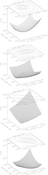 |
Fig. 2 χ2 values, in contour levels and 3D surfaces around the minimum values for 1667 MHz LCP (top), 1667 MHz RCP (from top to bottom), and 1665 MHz LCP and 1665 MHz RCP (bottom). |
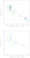 |
Fig. 3 Vobs−Vsys (with Vsys = 8.0 km s−1) versus the distance to the (α, δ)m point for the OH VLBA data shown (top). A clear trend is seen, where the velocity grows as the distance d(α,δ)m decreases. Same relation but for the VLA data of colour (bottom) taken from Argon et al. (2000). Symbols and colours are the same as in Fig. 1. |
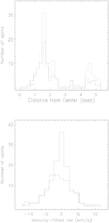 |
Fig. 4 Histogram of the number of spots (including the three frequencies) with the distance to (α, δ)m, dotted lines are for LCP and dashed for RCP (top). Histogram of the number of spots with velocity (bottom). Lines are as in the top panel. |
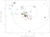 |
Fig. 5 Locations of the OH maser spots, observed with the VLBA, are indicated with small circles. These spots are the same as those plotted in Fig. 1 (also with circles). The asterisk represents the (α, δ)m point. The groups used to estimate the average velocity (Fig. 8) are indicated with vertical bars. The Argon et al. (2000) OH maser spots are indicated with triangles and the methanol maser cloudlets with crosses (×). All the methanol maser cloudlets that lie in this FOV (Bartkiewicz et al. 2014; Pandian et al. 2011) are on the west side, clumped together near the large dashed circle. |
3 Methanol maser cloudlets
We compared the locations of the methanol masers, observed by Bartkiewicz et al. (2014) and by Pandian et al. (2011), in W49N with those of the OH maser spots, and their velocities are analysed to look how they fit in the model proposed for OH spots. The Bartkiewicz et al. (2014) observations were set to four pointing positions. The coordinates (J2000) of the brightest spot at each position are given in their Table 2. The masers detected at W49N are spread over an area of 1.3′×0.9′. In their Table B.1, the locations of the spots are given as angular offsets (in mas) with respect to the location of the brightest spot of each group. The G43.165+00.013 group, which contains 12 spots, is the only one that lies in the FOV of the OH VLBA masers. The coordinates of the brightest spot of this group are α = 19:10:12.882 and δ = 09:06:12.2299. Using the coordinates of this spot and the offsets of the other spots of the group (with respect to the former), we obtained their corresponding α and δ (J2000). Then, with these coordinates and the coordinates of the OH reference point (α = 19:10:13.2091, δ = 09:06:12.485), the spot coordinates were transformed to offsets, but now with respect to the OH VLBA reference.
The Pandian et al. (2011) methanol maser observations also were made to different pointing positions, whose locations span to more than 1′ in both, α and δ. The locations of the spots are given in absolute coordinates in their Table 3. Only the G43.16+0.02 maser spot, lies in the FOV of the OH masers. Its location coincides with the above-mentioned Bartkiewicz et al. (2014) group (bottom panel of Fig. 6). To transform these coordinates into offsets, with respect to the OH reference point, we subtracted the OH reference coordinates from the Pandian et al. (2011) coordinates of the spot.
The observations of Bartkiewicz et al. (2014) were made with a very high angular resolution (of ~5 mas). Among the parameters that they report, here we use the above-mentioned offsets (RAoffset, Decoffset), the velocity of the peak flux (Vpk) and the velocity gradient (Vgrad), all of them for each spot. The last parameter is the velocity variation at the different velocity channels, where the spot is detected, with respect to the coordinates at these velocities.
In Fig. 5, the locations of the methanol maser cloudlets are represented with crosses. The spots of both, Bartkiewicz et al. (2014) and Pandian et al. (2011) data are clumped together in the west, near the large dashed circle.
The OH VLBA field is 6″ × 6″, which is small compared to the whole area of the Bartkiewicz et al. (2014) spots at W49N and of the field of the Pandian et al. (2011) one. This is to say that even if the distance between the centres of the fields is approx 5″, the methanol fields are much larger than the OH one and many of the methanol cloudlets, as reported by Bartkiewicz et al. (2014) and by Pandian et al. (2011) lie outside the field of the OH spots.
The peak velocities, Vpk, of the Bartkiewicz et al. (2014) maser spots spread from about 8 to 20 km s−1. The range of velocities and the high spatial resolution allows us to do the same process as that for OH spots. A mesh of points, separated ∆α = 10 mas, from −4500 to −5100 mas in right ascension (RA) and separated ∆δ = 10 mas from −600 to 0 mas in Declination (Dec) was used. The correlation and the χ2 between Vpk and distance are estimated to each point of the mesh for the 12 spots mentioned by Bartkiewicz et al. (2014). We further refer to C(α,δ)mMeth as the point for which the highest correlation is attained. In the top panel of Fig. 6, we show a plot of Vpk-Vsys, with Vsys = 8 km s−1, where the systemic velocity estimated by Welch et al. (1987) against the distance (dccMeth) to C(α,δ)mMeth is shown. It may be seen that the velocity undergoes a gradient with a negative slope (as in the case of OH masers). Similarly to the procedure with OH data, a straight line with velocity Vftd is fitted to these data. The Vpk−Vsys against distance to C(α,δ)mMeth values for the Pandian spot are also plotted with a rhombus.
In the bottom panel of Fig. 6, the locations of the methanol maser cloudlets of the G43.165+00.013 group from Bartkiewicz et al. (2014) are indicated by crosses (×). The sizes of the symbols are proportional to the Vpk−Vsys velocities. The rhombus in the N corresponds to the Pandian et al. (2011) spot. The point C(α,δ)mMeth is indicated with the plus symbol (+). The dashed circles are plotted for reference at distances from C(α,δ)mMeth (30 and 130 mas), where more spots are seen. It may be seen from the bottom panel of Fig. 6 that the spots closer to C(α,δ)mMeth have higher velocities than the spots farther from it. Additionally, it is seen that spots located at different sectors of the small dashed circle have similar Vpk−VSys velocities. The velocity field indicates acceleration towards C(α,δ)mMeth.
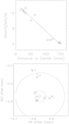 |
Fig. 6 Crosses indicate the Vpk−Vsys velocities against the d(α,δ)mMeth distances (to the point C(α,δ)mMeth) of the methanol cloudlets observed by Bartkiewicz et al. (2014), shown at the top. The rhombus indicates the Vpk-Vsys velocity against d(α,δ)mMeth of the Pandian et al. (2011) spot that lies in this FOV. Crosses (×) indicate the locations of the Bartkiewicz et al. (2014) methanol cloudlets and the rhombus, as well as the Pandian et al. (2011) methanol cloudlet, all of them given as offsets in asec, with respect the OH VLBA reference coordinates, shown at the bottom. The size of the symbols is proportional to the velocity. The cross (+) indicates the location where the maximum correlation between Vpk−Vsys and the distance d(α,δ)mMeth is attained. The distance, d(α,δ)mMeth, used in the top-panel plot is computed from this point. Dashed circles are plotted for reference at 30 and 130 mas from C(α,δ)mMeth. |
4 Discussion
The velocity field in 3D could be reconstructed by using both the radial velocity, Vobs, and the proper motions of the spots. However, in this case, we did not have access to this last information. Nevertheless, the fact that there is a region, in the field, for which the correlation between Vobs and the distance to that region, d(α,δ)m, takes the largest values, among all the points of the field; this indicates that the behaviour of the velocity field is more clearly revealed because it is probably a location the behaviour of this velocity field is dependent on. In other words, it is a parameter involved in a functional relationship between Vobs and d(α,δ)m.
For Keplerian rotation, the velocities in the E and W sectors, with respect to the systemic velocity, are opposite to each other and the velocities in the N and S are near to the value of the systemic velocity, as can be seen at single sources. From Figs. 3 and 5, it may be seen that none of these characteristics is present in the OH spots in W49N. Nevertheless, a series of tests of the locations and velocities of the sources was made with a geometric method, which allows us to compare them with ellipses, which are due to inclined Keplerian rotation orbits (Rodríguez-Esnard 2011). In Appendix A, the bases of the method to test the fit of the spots to an ellipse are given. Applying it to OH maser data, it is found that only nine spots of the 1665 LCP and ten spots of the 1665 RCP provide a good fit to ellipses for Keplerian-rotation. However, the geometric elements of the ellipses (centre, major axism and eccentricity) differ considerably from each other. Finally, we conclude that the spots are not in a rotating disk.
It has been seen that Vobs shows a general trend along the whole field, indicating that the velocity of the masers, in this field, has a global component. With respect the (α, δ)m point, the spots are predominantly in the E sector, distributed in an elongated shape, NE – WS orientated. In other sources, accretion has been seen to take place through filaments (Peretto et al. 2013). However, the amount of material accreted through them is not as large as the amount accreted radially. In the case of the W49N, the highest correlation is observed between Vobs and dij (the distance to the point (α, δ)m) and not along the direction of the elongation. The OH spots with similar velocities are approximately at the same distance to (α, δ)m. For example, as above mentioned, the spots that are close to the reference circle plotted at 1.6 asec radius have similar velocities, although they are in different sectors. For the spots around the circle at 4.6 asec, the same situation is seen but these spots have lower velocities. The spots are likely in a global velocity field, which is consistent with an accelerating contraction towards the (α, δ)m point; this can be interpreted as global contraction towards a common centre (CC). The results obtained with VLBA observations are supported by the Argon et al. (2003) data, obtained with the VLA, the (α, δ)m, as these data only differ by 0.3 asec with respect to the point estimated with the VLBA data.
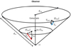 |
Fig. 7 Model of the contraction velocities, Vcc, of the OH spots, i.e. of their velocities towards a common centre of contraction (CC). Vftd (represented with dotted lines) corresponds to the velocity from the straight line fitted to the observed data for the given distance to (α, δ)m, as may be seen in Fig. 3. This velocity is assumed to be the radial component of the contraction velocity. Each spot has its own velocity (the two Vftd, represented here, are different to each other in magnitude). The small ellipse corresponds to the small circle plotted in Fig. 5. For an assumed spot at a point in this circle, |Vftd| is the magnitude of the transversal velocity, which is directed to the CONUS axis (and orientated perpendicular to it). The |Vftd| of the spot at the large ellipse is smaller than that at the small one. The resulting contraction velocity, of a magnitude, Vcc, lies on the surface of the CONUS and it is directed to the CC point (the apex of the CONUS). |
4.1 3D model of the contraction velocities
We recall that Vftd has a functional relation (fitted line in Fig. 3) to the distance to (α, δ)m. The shorter the distance to (α, δ)m the greater the Vftd. Then, given the distance to (α, δ)m, the corresponding Vftd velocity can be known. It is the same for all the points on a circle centred at (α, δ)m. These velocities can then be further used for the purposes of building a model. In Fig. 7, the Vftd velocity for two spots, one assumed to be at the distance of the small and the other of the large circles of Fig. 5 are shown. Each Vftd is considered to be the radial component of the contraction velocity to a common centre (Vcc). They differ from one another in magnitude and, ultimately, that the spot that is closer to CC has higher Vftd velocity than the spot that is farther from it. We consider the possibility that the CC is not on the same plane of the small circle (at Fig. 5). We assume that the Vcc of the two plotted spots and of all the spots are directed towards CC, which is at the apex of a CONUS, and all the Vcc vectors are located on the surface of the CONUS.
In the model, dxy is the distance from a spot to the CONUS axis (Fig. 7). In particular, for the plane of the small circle, this distance is equal to d(α,δ)m. Furthermore, the XY-plane of the small circle will be considered as a reference. It is represented with the small ellipse in Fig. 7. The distance to this plane is dz, it is positive as going farther from the observer and negative as it gets closer to the observer. In terms of the observed values, it may be seen that the spots that are at distances <1.6 asec, that is, closer to CC with respect to the small circle and farther from the observer would be at dz > 0; the spots that are at distances >1.6 asec, namely, farther from CC and closer to the observer would be at dz < 0 (Fig. 7). The CC is in the line of sight of the point (α, δ)m at a distance, dz0. The angle between the CONUS axis and the line from a spot to the CC is indicated with θ.
The tangential component of Vcc is unknown. Then, for the model, the following assumptions are as follows: (1) the tangential component of Vcc follows the same functional relation with the distance as the radial component with the distance to (α, δ)m. We remember that in the z-direction, the distance to CC is dz (Fig. 7); (2) it is orientated perpendicular to the CONUS axis and it directed to it. In the case of spots on the small circle of Fig. 7, this velocity is pointing to (α, δ)m. (3) It can be considered, for simplicity, that the tangential component of Vcc has a magnitude equal to |Vftd|. In the representation of Fig. 7, each point on the CONUS has its own velocity  , pointing in a radial direction (respect the observer) and their own tangential velocity,
  (pointing to the CONUS axis), and the vector Vcc would be the sum of them. Furthermore, these velocities are not written in vectorial notation, since in the model, each of them displays a clear orientation and sense, as may be seen from Fig. 7.
With the above-listed conditions on the contraction velocities, we can assume that the distance of a spot to the CONUS axis (dxy), which is measured perpendicular to the axis, would be the same as the distance in the radial direction (dz) and thus θ = 45°. This means that for the plotted spots (and any spot overall even if it does not lie at any of the two circles), the result will be dz = dxy. The distance of each spot to CC is thus  . The distance, dcc, is measured from CC to the spot. In the model (Fig. 7), the distance, dcc, to a spot that lies within the dashed circle, namely, at a distance of 1.6 asec, is indicated. If another spot does not lie at this distance, then it will not be at the dashed circle; however, it will be over the CONUS and its infalling velocity (due to global contraction) that is given for the linear fit of Fig. 3. The tangential velocity also depends on θ, which is the aperture of the CONUS. For θ = 45°, its magnitude is |Vftd| and then
  .
.
Besides the Vcc values, the velocity of each spot also could have random or local kinematics components. However, the difference ∆V = (Vobs−Vsys)−Vftd (Fig. 3) represents only the radial component of this velocity. To include a reasonable input to the random or local kinematics velocity in a tangential direction, we compute it in the same way as for Vftd. Then, taking into account that θ = 45°, the estimation of a total velocity for each spot leads to  . The total velocity is plotted in Fig. 8.
The average velocity of groups of spots located near each other is an estimate of the group velocity and this would reduce the impact of local kinematics or random velocities in the data dispersion. This could allow us to see how the group velocity versus dcc would behave, with regard to the case of separated spots. The groups of spots that we used are indicated with the vertical lines in Fig. 5. The average of the velocity of each group is shown with diamonds in Fig. 8, together with the velocity of separated spots (crosses). It may be seen that they behave similarly to each other, showing a maximum at about log(dcc) = −0.9(~0.12 pc). A general velocity increase is seen, which is rather noisy nonetheless, as a trend from 0.19 to 0.12 pc. On the other hand, a general decrease from 0.12 pc to shorter distances is also seen. For the computation of the infall velocity field, we considered the 0.42−0.19 pc interval. For the infall velocity, we use the value fitted to  at 0.19 pc, which is 10.7 km s−1.
We recall that the velocity difference (∆V) is the result of subtracting the fitted velocity, given by the straight line of Fig. 3 from the observed velocity. Therefore, ∆ V is related to components, of the spot velocity, which is different to the infalling velocity. In Fig. 9, the velocity difference, ∆ V versus Vobs is plotted. The closer a spot is to CC, the smaller the symbol that represents its velocity. Different symbols correspond to spots at different distance intervals. The spots grouped in a given distance interval are fitted by the same straight line. This occurs even though the spots are located at different sectors with respect to a centre point, which in this case, is CC. The small crosses represent the closest spots to (α, δ)m, while small circles represent the spots that are next in terms of the distance and so on. The spots around the continuous line correspond to the velocity increase seen from 0.19 to 0.12 pc. As may be seen from this figure, these lines show the largest velocity dispersion. They belong to different groups of Fig. 5, some of them located in the east, others in the south, and some in the north-west. The spots at d < 0.12 pc also belong to various groups of Fig. 5 in different sectors. They seem to be experiencing a deceleration as approach CC (Fig. 8). This could be similar to the case of a single protostar model (Stahler et al. 1980) in the sense that it could be accretion in a structured shape, including different layers. In the case of global collapse, there is no such detailed scheme. However, here we do not attempt to study these details in this work.
To estimate the free fall time, we assumed n = 1×10⁻⁴ cm−3 and an average mass particle 〈m〉 = 2.33 mH (Kauffmann et al. 2008, 2013), obtaining a result of tff = 3.4×10⁵ yr. The accretion rate, assuming a spherical geometry, can be calculated from 2πrρVinfall, for a distance of 0.19 pc and ρ from the above estimation, we have an accretion rate of 1.4× 10⁻³ M⊙ yr−1. Considering this accretion rate, the time required to accumulate a mass of 2500 M⊙ is 1.8×10⁶ yr, which is 5.2 times tff.
Part of the inner mass is in the cores and stars embedded in HII regions. Smith et al. (2009) found that several radio sources are deeply embedded inside the cloud core. Also, part of the mass could take the form of stars that already have swept out their HII regions and could be not detectable in the radio continuum and other wavelengths.
To estimate the virial coefficient, it must be taken into account that the velocity dispersion is due to global and to local kinematics. We calculated the virial mass, Mvir, using the standard deviation of ∆V, which turns out to be 2.9 km s−1 and leads to Mvir = 380 M⊙. It is smaller in more than six times Minn, which is the mass obtained by fitting the free-fall function to the Vcc values.
Rudolph et al. (1990) estimated a global collapse in W51 with a mass of 4×10⁴ M⊙ and a 1200 M⊙ subcollapse. The field of the OH spots in W49N has a side of approximately ~7 asec, while the ring of Welch et al. (1985) for W49N is ~20 asec. This means that the smaller region is virialized by itself, even though it is a fraction ~(7/20)3 of the Welch ring of HII regions. However, the kinematics of the smaller region spans a velocity range similar to the velocity range of the ring. The global velocity field of OH masers could be due to a sub-collapse similar to that observed in W51.
The analysed group of methanol cloudlets show similar conditions, in velocity and location, to those seen in the OH masers, allowing us to apply them to the same model (with another centre of contraction). It should be noted, however, that only one OH maser spot (indicated with a circle in the right panel of Fig. 6) is co-spatial to the methanol cloudlets. This means that the OH spots do not trace this region. Sanna et al. (2010b) studied the high-mass star-forming region G23.01-0.41 and found that the OH spots are more distant from the YSO than the methanol ones. Here, the only OH spot, which is co-spatial to this group, is certainly in the external region with respect to CCMeth.
The velocity gradient, seen at a group of methanol cloudlets, could be related to the kinematics of the source. In the top panel of Fig. 10, the velocity gradient, Vgrad, of each spot is plotted against its distance to CCMeth. It may be seen that the values of Vgrad at ~500 AU (near to the small dashed circle) have a larger dispersion than the spots at ~2000 AU (near to the large dashed circle). We should not exclude the possibility that near to CCMeth, another kinematical component, such as a disk, jet, or outflow that has been traced in other sources with methanol masers (Pandian et al. 2011; Moscadelli et al. 2011), could be present. That scenario would lead to larger dispersion in the velocity field in this region and a larger difference in the velocity from one spot to another than in regions that undergo a single type of kinematics.
Only one Pandian et al. (2011) methanol maser cloudlet lies in the field of OH spots, which is coincident with the Bartkiewicz et al. (2014) methanol cloudlets. They are located in the west of the VLBA field (crosses (×) The velocity of the Pandian et al. (2011) spot is Vpk = 9.3 km s−1 which, taking into account Vsys = 8 km s−1, gives us Vpk−Vsys = 1.3 km s−1. This velocity is similar to those of the OH spots located at similar distances from CCOH. The values (velocity and distance) for this spot are also plotted in Fig. 6. The rhombus that represents it (in the top panel) lies near the straight line fitted to the velocity versus distance plot, for the Bartkiewicz et al. (2014) spots.
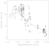 |
Fig. 8 Estimated total velocity, VTot, of the OH spots to the centre of contraction, as a function of the distance to CC, dcc. The crosses (×) denote the average velocities for the groups indicated with bars in Fig. 5. The dashed line denotes the free fall velocity for Minn = 2500 M⊙. |
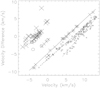 |
Fig. 9 Velocity difference (∆ V) versus Vobs. Different symbols correspond to spots at different distance intervals. The small crosses are for dcc < 0.09 pc, the dashed line is fitted to these spots. The small circles are for spots at 0.09 pc < dcc < 0.12 pc, and the dotted line is fitted to them. The continuous line is fitted to spots at 0.12 pc < dcc < 0.19 pc, which is shown with mid-size crosses. The large circles are for 0.19 pc < dcc< 0.25 pc and large crosses for 0.25 pc < dcc < 0.42 pc. |
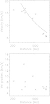 |
Fig. 10 Velocity VTMeth versus the distance, of each methanol cloudlet seen at the W in Fig. 5, to dccMeth shown on top. The dashed line corresponds to the free-fall velocity for a 75 M⊙ inner mass. The Vgrad velocity of each methanol cloudlet versus the dccMeth distance (bottom). |
4.2 Contraction of the group of methanol maser cloudlets
Velocity gradients are expected to be observed in different kine-matical models. In the case of maser spots in a rotating disk, the spots with more red- and more blue-shifted velocities would be observed, from the Earth, at both sides of the central region. The locations at W49N of methanol cloudlets with similar velocities, in different sectors (small dashed-circle of the right panel of Fig. 6), differ from what is expected in a rotating disk. Instead, this indicates that another type of kinematics is responsible for spots with such velocities and locations. The expansion or contraction is suitable to explain both conditions, with respect to a given centre. A third condition, namely, the larger velocities seen closer to the C(α,δ)mMeth point, agree with accretion in an accelerated velocity field.
The velocity versus distance relation of the methanol maser cloudlets seen at the FOV of the OH VLBA maser spots (Fig. 6) also suggests a centre of contraction for this particular group. A model of contraction is applied in a similar way as in the case of OH spots (Sect. 4.1 and Fig. 7). We assume that the distance in the direction perpendicular to the XY-plane, from each spot to CCMeth, is the same as the distance, d(α,δ)Meth, from the spot to C(α,δ)mMeth. Then, the distance of each spot to this point is  and we consider that the total velocity is
  . The first term corresponds to the falling velocity (towards CCMeth) and the second to the dispersion velocity, with respect to the falling one.
In the top panel of Fig. 6, the velocity, VTMeth, is plotted against dccMeth. Taking the interval of distances from 300 to 2500 AU, a free-fall function is fitted to Vpk−Vsys versus dccMeth (dashed line in the top panel of Fig. 10), obtaining an inner mass of 75 M⊙. This approximation helps us to estimate the inner mass, under the assumption of accretion. In this case, it is a region on a smaller spatial scale than that of the OH maser spots, indicating the possibility of another sub-collapse (that could contain various forming stars or one massive forming star).
The amount of methanol cloudlets in the W49N field, where the OH masers are seen, is smaller than the OH spots number. The methanol cloudlets are at given locations of the whole region, while the OH ones are more spread, namely, they appear in more locations across the region. This result agrees with the previous finding that 6.7 GHz methanol masers trace early phases of the high-mass star formation process (Minier et al. 2005; Pandian et al. 2011). The methanol masers could be more suitable to trace the velocity of the environment of such objects, providing the opportunity to study their kinematics. This also indicates that the OH and methanol masers seem to be complementary to each other in the study of star formation rates (SFR, Sanna et al. 2010b).
The locations and velocities of methanol masers do not disagree with a scenario of a subcollapse in W49N, as deduced from OH masers. Moreover, their velocities and locations agree with accretion scenarios at shorter spatial scales, which could indicate the possibility of sub-collapses on these scales. The combination of both maser species, therefore, seems to be a tool that is useful in building a more complete picture of the kinematics of SFR on different spatial scales, particularly in large complexes such as W49N.
As opposed to the case of the OH and the methanol maser spots analysed here, which trace contractions, the H2O maser spots at W49N, trace outflows. The bipolar outflow is related to the local kinematics at the G1 HII region and the velocity range of the H2O maser spots is considerably larger than the global field velocity range estimated by Welch et al. (1985) and also for the one analysed here. This means the H2O spots are related to local conditions at a given HII region, while the OH maser spots are related to the global kinematics.
5 Conclusions
The maximum correlation between the observed velocity, Vobs, and the distances to test points, dij, takes values larger than 0.7 for 1665 (RCP and LCP) and 1667 (RCP and LCP). Using the distance of the spots to the weighted average coordinates (α, δ)m, of the maxima of the correlation, the location of the projection of the centre of contraction to the XY-plane is estimated as (α2000 = 19:10:13.1253, δ2000 = 9:6:13.570). It is found that the behaviour of  against dcc shows a maximum at 0.12 pc, with a decrease from 0.12 to 0.19 pc that takes place faster than the decrease between 0.19 and 0.42 pc. Assuming that the behaviour of the velocity at the 0.19 and 0.42 pc interval is due to free fall accretion, an inner mass of Minn = 2500 M⊙ is obtained. We estimate the accretion rate to be
  which requires a time tinn = 1.8×10⁶ yr to accumulate Minn. The velocities of the OH spots at W49N, together with their positions with respect to the (α, δ)m point, makes it possible to estimate the spot kinematics. Finally, this can be interpreted as a contraction of the cloud that appears to be a sub-collapse in the W49N MC.
Acknowledgements
We would like to thank the Astrophysics Department of INAOE for its financial support. M-T. J.E. would like to acknowledge M. Goss for providing the VLBA data of 2005. We also thank the anonymous referee for her/his careful review of the present article and helpful suggestions, which have been very useful to us for improving this work.
Appendix A Model of ellipse
To test if the observed positions of the maser spots fit into a model of an ellipse, the equation of the conic is used, given as follows:
 (A.1)
(A.1)
where χi and yi are, respectively, the observed RA and observed Dec. of the spots. The coefficients aij determine the output parameters of the geometric model. The second-degree coefficients a11, a22 and a12, determine whether the function is an ellipse or not, a12 is the rotation coefficient, while a01 and a02 are the translation coefficients (Apostol 2001). Furthermore, we provide a basis for testing whether the spot locations can fit an ellipse, based on Equation A.1.
In the teotherical case, for a non-degenerate conic, G=0. In an experimental situation, the better a model fits the observed values (χi and yi), the smaller will be G. Then, the coefficients have to be selected such that G takes the smallest possible value. To find the aij- values that lead to the best fit, the least-squares method is used. With this purpose, the python function leastsq is applied, from the optimize package inside the scipy python module and pylab interface for the use of the matplotlib library. To find the coefficient for the best fit, at least six spots are needed.
The least-squares method minimizes the value of S2, given by:
 (A.2)
(A.2)
where ∊i is the estimated uncertainty given as  , with ∊ix the uncertainty in xi and ∊iy the uncertainty in yi, Np is the number of parameters for the fit, N is the total amount of spots, and N-Np is the number of degrees of freedom.
The Equation A.1 can be expressed in matrix form as:
![Mathematical equation: $ G = \left( {\matrix{ 1 & x & y \cr } } \right)\,\left[ {\matrix{ {{a_{00}}} & {{{{a_{01}}} \over 2}} & {{{{a_{02}}} \over 2}} \cr {{{{a_{10}}} \over 2}} & {{a_{11}}} & {{{{a_{12}}} \over 2}} \cr {{{{a_{20}}} \over 2}} & {{{{a_{21}}} \over 2}} & {{a_{22}}} \cr } } \right]\,\left( {\matrix{ 1 \cr x \cr y \cr } } \right) $](/articles/aa/full_html/2023/01/aa40244-20/aa40244-20-eq19.png) (A.3)
(A.3)
and the matrix will be further referred to as A, which can be expressed as:
![Mathematical equation: $ A = \sum\limits_{i = 0}^2 {\sum\limits_{j = 0}^2 {{a_{ij}}} = } \left[ {\matrix{ {{a_{00}}} & {{{{a_{01}}} \over 2}} & {{{{a_{02}}} \over 2}} \cr {{{{a_{10}}} \over 2}} & {{a_{11}}} & {{{{a_{12}}} \over 2}} \cr {{{{a_{20}}} \over 2}} & {{{{a_{21}}} \over 2}} & {{a_{22}}} \cr } } \right] $](/articles/aa/full_html/2023/01/aa40244-20/aa40244-20-eq20.png) (A.4)
(A.4)
The condition for a non-degenerate conic is that det(A) ≠ 0 and the condition for having an ellipse is that  . From A, we can take a submatrix A0 as follows
![Mathematical equation: $ {A_0} = \left[ {\matrix{ {{a_{11}}} & {{{{a_{12}}} \over 2}} \cr {{{{a_{21}}} \over 2}} & {{a_{22}}} \cr } } \right]. $](/articles/aa/full_html/2023/01/aa40244-20/aa40244-20-eq22.png) (A.5)
(A.5)
Then, considering that a12 = a21, the condition for an ellipse is det(A0) > 0. Further, a description of the process to find the elements of an ellipse is made. It is based on Apostol (2001), where similar cases are studied1. The reduced equation of the ellipse (from the general Equation A.1), after a rotation and a translation, is:
 (A.6)
(A.6)
where χ′ and y′ are the rotated values (from observed RA and Dec., respectively), λ1 and λ2 are the eigenvalues of A0 (here, λ1 is the eigenvalue with the lowest absolute value, since it is inversely proportional to a, with a as the major semiaxis, and λ2 is inversely proportional to the minor semiaxis, b), and g00 is given by:
 (A.7)
(A.7)
If Equation A.6 is divided by −g00 we obtain
 (A.8)
(A.8)
Equation A.8 can be expressed in a convenient form to get it in the standard ellipse formula, as follows:
 (A.9)
(A.9)
To diagonalize A0 and eliminate the rotation terms, with the aim to determine the eigen values, λ1 and λ2, the following equation is used (Apostol 2001):
 (A.10)
where I is the identity matrix and Tr(A0) is the trace of the matrix A0. The solution of the quadratic Equation A.10 yields two values, namely, λ1 and λ2. On the other hand, it may be seen from Equation A.9 that the minor and major axis are given in terms of the eigen values as:
 (A.11)
and
 (A.12)
where the eigenvalues λ1 and λ2 are found from Equation A.10 by using the A0 matrix and, consequently, the aij values that lead to the minimum of S2 in Equation A.2. These are the values that give the ellipse of the best fit.
The centre of the ellipse, (x0, y0), can be found from Equation A.1. Substituting the translation equations x = x′ + x0 and y = y′ + y0 into Equation A.1, and assuming it its equals zero, we have:
 (A.13)
Then, setting the terms related to the translation equal to zero, that is, the coefficients of x′ and y′, it follows that
 (A.14)
and
 (A.15)
The values of x0 and y0 can be found by using the values of the model of the ellipse, which lead to the best fit, then solving the system of Equations A.14 and A.15, which correspond, respectively, to the second and third rows of the matrix A.
Finally, the inclination angle (θ) is given as (Wooton 1985):
 (A.16)
which can be found by using the values for the best fit.
References
- Argon, A. L., Reid, M. J., & Menten, K. M. 2000, ApJS, 129, 159 [Google Scholar]
- Argon, A. L., Reid, M. J., & Menten, K. M. 2003, ApJ, 593, 925 [NASA ADS] [CrossRef] [Google Scholar]
- Bartkiewicz, A., Szymczak, M., & van Langevelde, H. J. 2014, A&A, 564, A110 [NASA ADS] [CrossRef] [EDP Sciences] [Google Scholar]
- Bloemhof, E. E. 2000, ApJ, 533, 893 [NASA ADS] [CrossRef] [Google Scholar]
- Bloemhof, E. E., Reid, M. J., & Moran, J. M. 1992, ApJ, 397, 500 [NASA ADS] [CrossRef] [Google Scholar]
- Bonnell, I. A., Bate, M. R., & Vine, S. G. 2003, MNRAS, 343, 413 [NASA ADS] [CrossRef] [Google Scholar]
- Commerçon, B., Hennebelle, P., & Henning, T. 2011, ApJ, 742, L9 [CrossRef] [Google Scholar]
- De Pree, C. G., Mehringer, D. M., & Goss, W. M. 1997, ApJ, 482, 307 [Google Scholar]
- De Pree, C. G., Wilner, D. J., Goss, W. M., et al. 2000, ApJ, 540, 308 [NASA ADS] [CrossRef] [Google Scholar]
- De Pree, C. G., Wilner, D. J., Mercer, A. J., et al. 2004, ApJ, 600, 286 [NASA ADS] [CrossRef] [Google Scholar]
- Deshpande, A. A., Goss, W. M., & Mendoza-Torres, J. E. 2013, ApJ, 775, 36 [NASA ADS] [CrossRef] [Google Scholar]
- Dreher, J. W., Johnston, K. J., Welch, W. J., et al. 1984, ApJ, 283, 632 [NASA ADS] [CrossRef] [Google Scholar]
- Fish, V. L., & Reid, M. J. 2007, ApJ, 670, 1159 [NASA ADS] [CrossRef] [Google Scholar]
- Fish, V. L., Gray, M., Goss, W. M., et al. 2011, MNRAS, 417, 555 [NASA ADS] [CrossRef] [Google Scholar]
- Galván-Madrid, R., Liu, H. B., Zhang, Z.-Y., et al. 2013, ApJ, 779, 121 [CrossRef] [Google Scholar]
- Gwinn, C. R. 1994, ApJ, 429, 253 [NASA ADS] [CrossRef] [Google Scholar]
- Gwinn, C. R., Moran, J. M., Reid, M. J., et al. 1989, The Center Galaxy, 136, 47 [NASA ADS] [CrossRef] [Google Scholar]
- Gwinn, C. R., Moran, J. M., & Reid, M. J. 1992, ApJ, 393, 149 [NASA ADS] [CrossRef] [Google Scholar]
- Gwinn, C. R., Bartel, N., & Cordes, J. M. 1993, ApJ, 410, 673 [NASA ADS] [CrossRef] [Google Scholar]
- Johnston, K. J., & Hansen, S. S. 1982, AJ, 87, 803 [NASA ADS] [CrossRef] [Google Scholar]
- Kauffmann, J., Bertoldi, F., Bourke, T. L., et al. 2008, A&A, 487, 993 [NASA ADS] [CrossRef] [EDP Sciences] [Google Scholar]
- Kauffmann, J., Pillai, T., & Goldsmith, P. F. 2013, ApJ, 779, 185 [NASA ADS] [CrossRef] [Google Scholar]
- Kent, S. R., & Mutel, R. L. 1982, ApJ, 263, 145 [NASA ADS] [CrossRef] [Google Scholar]
- Kulczak-Jastrzebska, M. 2017, ApJ, 835, 121 [CrossRef] [Google Scholar]
- Liu, T., Kim, K.-T., Wu, Y., et al. 2015, ApJ, 810, 147 [NASA ADS] [CrossRef] [Google Scholar]
- McKee, C. F., & Tan, J. C. 2002, Nature, 416, 59 [CrossRef] [Google Scholar]
- Minier, V., Burton, M. G., Hill, T., et al. 2005, A&A, 429, 945 [NASA ADS] [CrossRef] [EDP Sciences] [Google Scholar]
- Moscadelli, L., Sanna, A., & Goddi, C. 2011, A&A, 536, A38 [NASA ADS] [CrossRef] [EDP Sciences] [Google Scholar]
- Motte, F., Bontemps, S., & Louvet, F. 2018, ARA&A, 56, 41 [NASA ADS] [CrossRef] [Google Scholar]
- Myers, A. T., McKee, C. F., Cunningham, A. J., et al. 2013, ApJ, 766, 97 [NASA ADS] [CrossRef] [Google Scholar]
- Pandian, J. D., Momjian, E., Xu, Y., et al. 2011, ApJ, 730, 55 [NASA ADS] [CrossRef] [Google Scholar]
- Peretto, N., Fuller, G. A., Duarte-Cabral, A., et al. 2013, A&A, 555, A112 [NASA ADS] [CrossRef] [EDP Sciences] [Google Scholar]
- Rodríguez-Esnard, I.T. 2011, PhD Thesis, Universidad de Guanajuato, Mexico [Google Scholar]
- Rudolph, A., Welch, W. J., Palmer, P., et al. 1990, ApJ, 363, 528 [NASA ADS] [CrossRef] [Google Scholar]
- Sanna, A., Moscadelli, L., Cesaroni, R., et al. 2010, A&A, 517, A71 [NASA ADS] [CrossRef] [EDP Sciences] [Google Scholar]
- Sanna, A., Moscadelli, L., Cesaroni, R., et al. 2010, A&A, 517, A78 [NASA ADS] [CrossRef] [EDP Sciences] [Google Scholar]
- Serabyn, E., Guesten, R., & Schulz, A. 1993, ApJ, 413, 571 [Google Scholar]
- Smith, N., Whitney, B. A., Conti, P. S., et al. 2009, MNRAS, 399, 952 [NASA ADS] [CrossRef] [Google Scholar]
- Stahler, S. W., Shu, F. H., & Taam, R. E. 1980, ApJ, 241, 637 [NASA ADS] [CrossRef] [Google Scholar]
- Takefuji, K., Imai, H., & Sekido, M. 2016, PASJ, 68, 86 [NASA ADS] [CrossRef] [Google Scholar]
- Welch, W. J., Vogel, S. N., Plambeck, R. L., et al. 1985, Science, 228, 1389 [NASA ADS] [CrossRef] [Google Scholar]
- Welch, W. J., Dreher, J. W., Jackson, J. M., et al. 1987, Science, 238, 1550 [NASA ADS] [CrossRef] [Google Scholar]
- Wilner, D. J., De Pree, C. G., Welch, W. J., et al. 2001, ApJ, 550, L81 [NASA ADS] [CrossRef] [Google Scholar]
- Zhang, B., Reid, M. J., Menten, K. M., et al. 2013, ApJ, 775, 79 [Google Scholar]
- Zinnecker, H., & Yorke, H. W. 2007, ARA&A, 45, 481 [Google Scholar]
The involved equations are given in sections “Reduction from a real quadratic form to a diagonal form”, “Applications to analytical geometry” and in a number of examples and exercises.
All Tables
All Figures
|
Fig. 1 Map of the OH maser spots respect the reference coordinates. The (0,0) location corresponds to α = 19:10:13.2091, δ = 09:06:12.485 (J2000). Respectively, the dark and light blue circles represent the 1667 MHz LCP and RCP maser spots; green and yellow is for 1665 MHz LCP and RCP; and orange and red circles for 1612 MHz LCP and RCP. The crosses indicate the locations of HII regions, reported by De Pree etal. (1997), with the corresponding letters used to refer to each of them. The square that overplots to the cross, which represents G1, corresponds to the location of the centre of the bipolar outflow of Gwinn et al. (1992). |
| In the text | |
|
Fig. 2 χ2 values, in contour levels and 3D surfaces around the minimum values for 1667 MHz LCP (top), 1667 MHz RCP (from top to bottom), and 1665 MHz LCP and 1665 MHz RCP (bottom). |
| In the text | |
|
Fig. 3 Vobs−Vsys (with Vsys = 8.0 km s−1) versus the distance to the (α, δ)m point for the OH VLBA data shown (top). A clear trend is seen, where the velocity grows as the distance d(α,δ)m decreases. Same relation but for the VLA data of colour (bottom) taken from Argon et al. (2000). Symbols and colours are the same as in Fig. 1. |
| In the text | |
|
Fig. 4 Histogram of the number of spots (including the three frequencies) with the distance to (α, δ)m, dotted lines are for LCP and dashed for RCP (top). Histogram of the number of spots with velocity (bottom). Lines are as in the top panel. |
| In the text | |
|
Fig. 5 Locations of the OH maser spots, observed with the VLBA, are indicated with small circles. These spots are the same as those plotted in Fig. 1 (also with circles). The asterisk represents the (α, δ)m point. The groups used to estimate the average velocity (Fig. 8) are indicated with vertical bars. The Argon et al. (2000) OH maser spots are indicated with triangles and the methanol maser cloudlets with crosses (×). All the methanol maser cloudlets that lie in this FOV (Bartkiewicz et al. 2014; Pandian et al. 2011) are on the west side, clumped together near the large dashed circle. |
| In the text | |
|
Fig. 6 Crosses indicate the Vpk−Vsys velocities against the d(α,δ)mMeth distances (to the point C(α,δ)mMeth) of the methanol cloudlets observed by Bartkiewicz et al. (2014), shown at the top. The rhombus indicates the Vpk-Vsys velocity against d(α,δ)mMeth of the Pandian et al. (2011) spot that lies in this FOV. Crosses (×) indicate the locations of the Bartkiewicz et al. (2014) methanol cloudlets and the rhombus, as well as the Pandian et al. (2011) methanol cloudlet, all of them given as offsets in asec, with respect the OH VLBA reference coordinates, shown at the bottom. The size of the symbols is proportional to the velocity. The cross (+) indicates the location where the maximum correlation between Vpk−Vsys and the distance d(α,δ)mMeth is attained. The distance, d(α,δ)mMeth, used in the top-panel plot is computed from this point. Dashed circles are plotted for reference at 30 and 130 mas from C(α,δ)mMeth. |
| In the text | |
|
Fig. 7 Model of the contraction velocities, Vcc, of the OH spots, i.e. of their velocities towards a common centre of contraction (CC). Vftd (represented with dotted lines) corresponds to the velocity from the straight line fitted to the observed data for the given distance to (α, δ)m, as may be seen in Fig. 3. This velocity is assumed to be the radial component of the contraction velocity. Each spot has its own velocity (the two Vftd, represented here, are different to each other in magnitude). The small ellipse corresponds to the small circle plotted in Fig. 5. For an assumed spot at a point in this circle, |Vftd| is the magnitude of the transversal velocity, which is directed to the CONUS axis (and orientated perpendicular to it). The |Vftd| of the spot at the large ellipse is smaller than that at the small one. The resulting contraction velocity, of a magnitude, Vcc, lies on the surface of the CONUS and it is directed to the CC point (the apex of the CONUS). |
| In the text | |
|
Fig. 8 Estimated total velocity, VTot, of the OH spots to the centre of contraction, as a function of the distance to CC, dcc. The crosses (×) denote the average velocities for the groups indicated with bars in Fig. 5. The dashed line denotes the free fall velocity for Minn = 2500 M⊙. |
| In the text | |
|
Fig. 9 Velocity difference (∆ V) versus Vobs. Different symbols correspond to spots at different distance intervals. The small crosses are for dcc < 0.09 pc, the dashed line is fitted to these spots. The small circles are for spots at 0.09 pc < dcc < 0.12 pc, and the dotted line is fitted to them. The continuous line is fitted to spots at 0.12 pc < dcc < 0.19 pc, which is shown with mid-size crosses. The large circles are for 0.19 pc < dcc< 0.25 pc and large crosses for 0.25 pc < dcc < 0.42 pc. |
| In the text | |
|
Fig. 10 Velocity VTMeth versus the distance, of each methanol cloudlet seen at the W in Fig. 5, to dccMeth shown on top. The dashed line corresponds to the free-fall velocity for a 75 M⊙ inner mass. The Vgrad velocity of each methanol cloudlet versus the dccMeth distance (bottom). |
| In the text | |
Current usage metrics show cumulative count of Article Views (full-text article views including HTML views, PDF and ePub downloads, according to the available data) and Abstracts Views on Vision4Press platform.
Data correspond to usage on the plateform after 2015. The current usage metrics is available 48-96 hours after online publication and is updated daily on week days.
Initial download of the metrics may take a while.