| Issue |
A&A
Volume 668, December 2022
|
|
|---|---|---|
| Article Number | A174 | |
| Number of page(s) | 25 | |
| Section | Stellar atmospheres | |
| DOI | https://doi.org/10.1051/0004-6361/202244595 | |
| Published online | 21 December 2022 | |
Optimising the Hα index for the identification of activity signals in FGK stars
Improvement of the correlation between Hα and Ca II H&K
1
Instituto de Astrofísica e Ciências do Espaço, Universidade do Porto, CAUP,
Rua das Estrelas,
4150-762
Porto, Portugal
e-mail: This email address is being protected from spambots. You need JavaScript enabled to view it.
2
Departamento de Física e Astronomia, Faculdade de Ciências, Universidade do Porto,
Rua Campo Alegre,
4169-007
Porto, Portugal
Received:
25
July
2022
Accepted:
11
October
2022
Abstract
Context. The Ca II H&K and Hα lines are two of the most used activity diagnostics for detecting stellar activity signals in the optical regime, and for inferring possible false positives in exoplanet detection with the radial velocity method. The flux in the two lines is known to follow the solar activity cycle, and to correlate well with sunspot number and other activity diagnostics. However, for other stars, the flux in these lines is known to have a wide range of correlations, increasing the difficulty in the interpretation of the signals observed with the Hα line.
Aims. In this work we investigate the effect of the Hα bandpass width on the correlation between the Ca II and Hα indices with the aim of improving the Hα index to better identify and model the signals coming from activity variability.
Methods. We used a sample of 152 FGK dwarfs observed with HARPS for more than 13 yr with enough cadence to be able to detect rotational modulations and cycles in activity proxies. We calculated the Ca II and Hα activity indices using a range of bandwidths for Hα between 0.1 and 2.0 Å. We studied the correlation between the indices’ time series at long and short timescales, and analysed the impact of stellar parameters, activity level, and variability on the correlations.
Results. The correlation between Ca II and Hα, both at short and long timespans, is maximised when using narrow Hα bandwidths, with a maximum at 0.6 Å. For some inactive stars, as the activity level increases, the flux in the Hα line core increases, while the flux in the line wings decreases as the line becomes shallower and broader. The balance between these fluxes can cause stars to show the negative correlations observed in the literature when using a wide bandwidth on Hα. These anti-correlations may become positive correlations if using the 0.6 Å bandwidth. We demonstrate that rotationally modulated signals observed in SCa II, which appear flat or noisy when using 1.6 Å on SHα, can become more evident if a 0.6 Å bandpass is used instead. Low activity variability appears to be a contributing factor for the cases of weak or no correlations.
Conclusions. Calculating the Hα index using a bandpass of 0.6 Å maximises the correlation between Ca II and Hα, both at short and long timescales. On the other hand, the use of the broader 1.6 Å, generally used in exoplanet detection to identify stellar activity signals, degrades the signal by including the flux in the line wings. In view of these results, we strongly recommend the use of a 0.6 Å bandwidth when computing the Hα index for the identification of activity rotational modulation and magnetic cycle signals in solar-type stars.
Key words: stars: activity / planets and satellites: detection / techniques: spectroscopic / stars: solar-type
© J. Gomes da Silva et al. 2022
 Open Access article, published by EDP Sciences, under the terms of the Creative Commons Attribution License (https://creativecommons.org/licenses/by/4.0), which permits unrestricted use, distribution, and reproduction in any medium, provided the original work is properly cited.
This article is published in open access under the Subscribe-to-Open model. This email address is being protected from spambots. You need JavaScript enabled to view it. to support open access publication.
1 Introduction
As planet hunting instrumentation reaches higher precision levels, stellar activity becomes one of the most important limiting factors to exoplanet detection and characterisation. At short timescales of days to months, rotational modulation of active regions, zones of strong magnetic fields characterised by the presence of dark and cool spots and/or bright and hotter plages, create radial velocity (RV) quasi-periodic variations with timescales close to the rotational period, its harmonics, and that of active region life times, which can be of tens of rotational periods (e.g. Saar & Donahue 1997; Queloz et al. 2001; Santos et al. 2000, 2014; Boisse et al. 2009, 2011; Faria et al. 2020). At longer timescales of years and decades, activity variability similar to that of the 11-yr solar cycle is also known to affect RV and can interfere with the detection of long-period planets (e.g. Lovis et al. 2011; Gomes da Silva et al. 2012).
Several techniques to correct the effects of stellar activity on RV require the simultaneous measurement of activity proxies based on activity sensitive spectral lines (or using line shape indicators) to identify and remove activity effects on RV (e.g. Boisse et al. 2011; Dumusque et al. 2012; Rajpaul et al. 2015; Faria et al. 2022). The most widely used activity sensitive lines in the optical regime are the Ca II H&K and Hα lines. The flux in both lines is known to correlate with the presence of active regions and both are known to tightly follow the solar magnetic cycle (Livingston et al. 2007). However, studies of time series of indices based on the two lines for other stars have shown that the correlation between the indices is not straightforward: some stars show strong positive correlations, for others the two indices are not correlated, while a few show negative correlations (Cincunegui et al. 2007; Gomes da Silva et al. 2011, 2014; Meunier et al. 2022). Although the correlation between Ca II and Hα is not fully understood, some studies have found that the correlation tends to be strongly positive for stars with higher activity levels, while in the low-activity regime, all types of correlations are observed (Walkowicz & Hawley 2009; Gomes da Silva et al. 2011, 2014; Meunier et al. 2022).
Since the cores of the Ca II H&K and Hα lines are formed at different temperatures, and thus different heights in the chromosphere (e.g. Mauas & Falchi 1994, 1996; Mauas et al. 1997; Fontenla et al. 2016), we expect these two lines to trace activity phenomena differently. The different sensitivity of these lines to spots, plages, or filaments could explain the various correlations observed for different stars due to their varying filling factors, spatial distribution, and/or contrasts (e.g. Meunier & Delfosse 2009). Although some previous works have used a narrow bandpass of 0.678 Å to compute Hα (e.g. Kürster et al. 2003; Bonfils et al. 2007; Boisse et al. 2009; Santos et al. 2010), the majority of the recent studies of stellar activity, mainly in the context of exoplanet detection, have used broader bandwidths, usually of 1.6 Å. In fact, most studies of the correlation between Ca II and Hα, for FGK stars or the Sun, have also used a broad bandwidth to measure the Hα index (Cincunegui et al. 2007; Gomes da Silva et al. 2014; Maldonado et al. 2019; Meunier et al. 2022).
In this work we analyse the effect of changing the Hα bandpass width on the correlation between the flux in the Ca II and Hα lines, with the aim of maximising the correspondence between the two activity diagnostics and increasing the Hα sensitivity to stellar signals at short and long timescales. To our knowledge, this is the first time the impact of changing the bandwidth size of the Hα index is analysed for stars other than the Sun. In Sect. 2 we present our sample, and in Sect. 3 we explain how we calculated the Ca II and Hα indices. In Sect. 4 we expose our methodology to determine the correlation coefficients and their significance. We analyse the long-term correlations between Ca II and Hα in Sect. 5, and the short-term correlations in Sect. 6. A discussion of the results in terms of stellar parameters and activity variability, and an analysis of the Hα line wings are presented in Sect. 7, and we conclude in Sect. 8.
2 Sample and HARPS data
The sample was selected from the Gomes da Silva et al. (2021) catalogue of chromospheric activity of 1674 FGK stars from the High Accuracy Radial Velocity Planet Searcher (HARPS, Mayor et al. 2003) archive. This catalogue used more than 180 000 spectra to estimate precise and homogeneous mean activity levels and dispersion. The catalogue also includes stellar atmospheric parameters such as effective temperature, metallicity, and surface gravity, along with isochronal masses, radii, and ages. The HARPS instrument is a high-resolution, high-stability, fibre-fed, cross-dispersed echelle spectrograph with a resolution of λ/∆λ = 115 000 and a spectral range from 380 to 690 nm, mounted at the ESO 3.6 m telescope in La Silla, Chile. For a detailed description of the instrument we refer the reader to Pepe et al. (2002).
The main objective of the present work involves the comparison of the activity signals measured in the flux of the Ca II and Hα lines, and therefore our timespan and cadence need to cover the rotational modulation and activity cycles related variability for each star, if possible. To achieve this we need stars with a high number of observations and long timespans. We therefore selected, from the catalogue, the main sequence FGK stars with more than 60 days of observations and timespans longer than 1000 days. As we see in Sect. 6 and as can be observed in Fig. B.1, this selection enabled us to identify activity minima and maxima in magnetic cycles for most stars, and to have enough data points to use those epochs to compare the behaviour of our activity indices. Since some stars have very high cadences, characteristic of asteroseismology surveys, we imposed a maximum limit of 1000 spectra per star to reduce computational costs. Outliers were removed via a sequential 4-sigma clipping of the S Ca II, SHα 16, and SHα 06 indices’ time series (these indices are explained in Sects. 3 and 4). Since we are only interested in timescales longer than one day, all data were daily binned to mitigate high-frequency noise (Dumusque et al. 2011) and reduce the datasets. This selection resulted in a sample of 152 FGK dwarfs, including 101 G, 33 K and 18 F stars, with a total of 19 019 binned data points. Figure 1 shows the distributions of the number of binned observations and the timespan per star. The number of binned observations per star ranges between 61 and 458, with the median at 101, and the timespan ranges from 1437 days (3.9 yr) to 5531 days (15.1 yr), with the median at 4865 days (13.3 yr).
We also obtained stellar atmospheric parameters such as the effective temperature, Teff, metallicity, [Fe/H], and the median chromospheric emission ratio, log R′HK, from Gomes da Silva et al. (2021) and references therein. The distribution of these parameters for the sample are shown in Fig. 2 and their values are provided in Table C.1. The effective temperature varies between 4470 and 6732 K, with the median at 5694 K, the metallicity between −1.39 and 0.33 dex, with the median at −0.11 dex, and log R′HK ranges from −5.13 to −4.60 dex, with the median at −4.93 dex. Thus, the majority of our sample stars have about 100 days of observation on a timespan of almost 5000 days (~13.7 yr), and have effective temperature and activity levels similar to our Sun, with slightly sub-solar metallicity. These biases are due to the majority of these stars coming from exoplanet surveys targeting inactive, solar-type stars. Nevertheless, we should be able to assess the influence of these stellar parameters on the behaviour of the activity indices, if they are present.
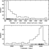 |
Fig. 1 Distribution of the number of observations (upper panel) and timespan (lower panel) per star. |
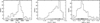 |
Fig. 2 Distribution of the effective temperature (left panel), metallicity (middle panel), and log R′HK activity level (right panel) for our sample. |
3 Activity indices based on the Ca II H&K and Hα lines
We used ACTIN1 (Gomes da Silva et al. 2018, 2021) to calculate the Ca II and Hα indices for the full sample. ACTIN calculates indices by integrating the flux in the activity sensitive lines and dividing them by the flux in pseudo-continuum regions:
 (1)
(1)
where Fi is the flux in the activity line i, N is the number of activity lines (e.g. for Ca II N = 2, for Hα N = 1), Rj is the flux in the pseudo-continuum region j, and M the number of pseudo-continuum regions. Generally there are two pseudo-continuum regions (M = 2) surrounding the activity lines in the redder and bluer nearby continuum. ACTIN uses linear interpolation to deal with the finite wavelength resolution of the spectrograph when integrating the flux over a given bandpass. For more information related to the flux determination and errors, we refer the reader to Gomes da Silva et al. (2021, Appendix A).
The Ca II index, which comes preinstalled in ACTIN, was measured following the procedure in Gomes da Silva et al. (2021), which mimics the original Mt. Wilson S-index derivation by Vaughan et al. (1978). In the case of Hα, we used the reference lines from Gomes da Silva et al. (2011) but computed the index for a range of central bandwidths between 0.1 and 2.0 Å, in steps of 0.1 Å. Since we are not comparing the values of these indices between different stars, only the correlations between them, the temperature-dependent photospheric contribution and bolomet-ric correction are not required. To compare the activity levels of stars, we used the usual log R′HK indicator (Noyes et al. 1984; Rutten 1984). From here on, we refer to the spectral lines as Ca II and Hα, and to the indices as SCa II and SHα.
4 Correlation coefficients and significance
As a metric for correlation, we chose the Spearman coefficient over the Pearson coefficient, so that we could infer correlations that are monotonic, either linear or not. Furthermore, the Spearman coefficient does not require the two datasets to be normally distributed, as is the case where we have correlated time series with signals such as the quasi-periodic modulation due to activity. The Spearman correlation coefficient, ρ, was calculated for SCa II and each SHα using a different bandwidth. To quantify the correlation significance, we calculated the p-value of the coefficients following the methodology described in Figueira et al. (2013)2. Briefly, for each star, we performed Fisher-Yates shuffling of the data pairs (SCa II and SHα) 10000 times to create unbiased and uncorrelated datasets, for which we calculated the correlation coefficients. The original correlation coefficient (before shuffling) was then compared with the mean of the shuffled population correlation coefficients, and the original dataset z-score was calculated. The p-value, the probability of having an equal or larger correlation coefficient under the null hypothesis that the data pairs are uncorrelated, was obtained from the one-sided probability of having such a z-score from the observed Gaussian distribution.
To compare values of the coefficients for narrow and wide bands, we used two representative bandwidths. As referred to in the introduction, the most used Hα bandwith to calculate the Hα index is the 1.6 Å bandpass. Due to its widespread use, we consider it as an example of a wide bandpass, and refer to this index as SHα16 from here on. As a reference to a narrow bandwidth, we use the Hα index calculated by integrating a 0.6 Å bandwidth, referred to as SHα063. For computational cost reasons, we only calculated the p-values for correlations using SHα06, SHα16, and SHα W (this last index is discussed in Sect. 7.3) both for the long- and short-term datasets.
From here on, we refer to ‘strong’ correlations if ρ has values higher than 0.5 in absolute value, and ‘weak or no correlation’ if ρ has values between −0.5 and 0.5. For example, we can have strong correlations that are insignificant (p-value ≥ 10−3) or weak correlations that are significant (p-value ≤ 10−3). As we see in the following sections, for the long-term datasets, all the strong correlations are significant. However, that is not always true for the short-term datasets.
5 Long-term correlations
To investigate the correlation between SCa II and SHα at long timescales, we used the full time series for all stars. The Spearman correlation coefficients and their p-values when using band-pass widths of 0.6 and 1.6 Å, as well as using the Hα line wings between 1.6 and 0.6 Å (see Sect. 7.3), are provided in Table C.2.
5.1 Correlations for different Hα bandwidths
We expect the correlation between Ca II and Hα to vary with the Hα bandwidth used because different depths of the Hα line probe different heights of the stellar atmosphere. Figure 3 shows the Spearman correlation coefficients as a function of Hα bandwidth coloured after activity level. In the upper panel, we show only the stars having strong positive or negative correlations (ρ ≥ 0.5 and ρ ≤ −0.5) using the 0.6 Å bandwidth as an example of a narrow bandpass, while in the lower panel only stars with weak or no correlations (−0.5 < ρ < 0.5) with SHα06 are represented. In the case of SHα06 and SHα16, all stars with |ρ| ≥ 0.5 also have p-values ≤ 10−3, meaning that all those correlations are statistically significant. As a first observation, we see a tendency for the correlation to decrease as the Hα bandwidth increases. Four different behaviours of the correlation as a function of bandwidth can be observed: (1) ‘flat-positive’, where the correlation is strong positive and almost constant across bandwidths; (2) ‘positive-zero’, where it decreases from strong positive to weak or no correlation; (3) ‘positive-negative’, where it decreases from strong positive to strong negative; and (4) ‘flat-negative’, where it is constant but always strong negative. The figure also provides other interesting information: (i) all cases of strong positive SCa II–SHα16 correlation also have strong positive SCa II–SHα06 correlation (upper panel), and there are no cases where the correlation increases from weak to strong with increasing bandpass width; (ii) all cases of strong negative SCa II–SHα16 correlation have strong positive SCa II–SHα06 correlation, except for HD 206998 (upper panel), narrow bandpasses can turn strong anti-correlations into strong positive correlations; (iii) all cases of weak or no correlation between SCa II and SHα06 also show weak or no correlation between SCa II and SHα16 (lower panel), these stars never show strong correlations between the calcium and hydrogen lines, regardless of the Hα bandwidth used; (iv) the only case of strong negative SCa II–SHα06 correlation, HD 206998, also has strong negative SCa II–SHα16 correlation (upper panel), since we only have one star in this situation, we cannot ascertain whether this is an outlier or an additional behaviour; and (v) in general, stars with lowercorrelations with SHα16 tend to have lower activity levels (upper panel), which is in agreement with Gomes da Silva et al. (2014); Meunier et al. (2022).
These behaviours show that, for most inactive4 FGK dwarfs, using a narrow Hα bandpass can improve the correlation between the Hα and Ca II indices, and that most of the anti-correlations detected between these two indices are caused by using a wide bandwidth when calculating the Hα index. It is also interesting to note that if a star has no correlation using SHα06, then widening the bandpass will not improve the correlation into either strong positive or negative values. In general terms, narrower bandwidths are preferred if one wants to detect activity signals similar to those followed by Ca II (which is known to correlate well with plages in the Sun and with activity induced RV).
In Fig. 4 we show three examples of the Hα profile for three cases represented in Fig. 3 (upper panel) in which all have similar SCa II–SHα06 correlation coefficients but behave differently as the Hα bandwidth is increased. To compare the Hα lines at maxima and minima, we normalised the spectra by the mean of the flux in the R1 and R2 pseudo-continuum regions used to compute the SHα index. In the left panel, we show HD 215152 (K3V), a star with a ‘flat-positive’ behaviour, in the middle panel, we show HD 20003 (G8V), a star showing ‘positive-zero’ behaviour, and in the right panel, we show HD 7199 (G9V), an example of a ‘positive-negative’ correlation behaviour. The top panels show the Hα line at the minimum (blue) and maximum (red) of SCa II activity for each star, while the bottom panels show the difference in flux between these extremes. The vertical lines in all figures represent the limits of the 0.6 Å bandwidth (dotted lines), the 1.6 Å (dashed lines), and the maximum bandwidth value we used of 2.0 Å (solid lines). The numbers in the lower panels show the flux difference calculated in each width, coloured red if positive (more flux at activity maximum) and blue if negative (more flux at activity minimum). The first thing we can observe in these examples is that the flux in the core always increases with SCa II activity level, while the flux in the wings can increase or decrease with activity level. We can see that, for the case of HD 215152 (left panel), as Ca II increases, both the Hα line core (between the 0.6 Å limits) and the lateral ‘wings’ of the lines increase in flux. Thus, the correlation between Ca II and Hα is positive, either using a narrow or a wider bandpass. On the other hand, in the case of HD 20003 (middle panel), while the difference in flux in the line core is positive as the activity increases, the line wings widen, and thus decrease in flux, producing a negative flux difference. This means that, while we get a positive correlation using a narrowband, as we increase the bandwidth, we start degrading the correlation by including the negative flux difference from the line wings, and the correlation drops to almost zero because the positive flux difference in the core and the negative flux difference in the wings almost compensate each other. If the broadening (the drop in flux) of the Hα wings is larger than the increase in flux in the core, as in the case of HD 7199 (right panel), the correlation can become negative when a wide bandpass is used. However, a strong positive correlation is still possible if a narrow bandwidth is used instead. A similar Hα profile behaviour was previously observed by Flores et al. (2016, 2018) while studying the activity cycles of the two solar analogues HD 45184 and HD 38858 (both included in our sample). While the Hα equivalent width showed no significant variability, the shape of the Hα profile produced variations compatible with the Call cyclic variations. In fact, their Hα profile core (<0.7 Å from centre) increased in flux with Ca II activity level, while the ‘wings’ flux decreased.
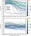 |
Fig. 3 Effect of varying the Hα bandwidth in the correlation between Ca II and Hα coloured after activity level, measured as logR′HK. Upper panel: stars with strong positive (ρ ≥ 0.5) or negative (ρ ≤ −0.5) correlation with the SHα06 index. Stars marked with thick lines are examples used in Figs. 4, 7, and A.2, and the only case of negative correlation with SHα06 (HD 206998). Lower panel: stars with weak or no correlation (−0.5 < ρ < 0.5) with the SHα06 index. In both panels, as an indication, we mark the boundaries between strong and no correlation with horizontal dotted lines at ρ values of 0.5 and −0.5. |
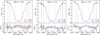 |
Fig. 4 Flux in the Hα line for different levels of activity. Upper panels: Hα line profiles of HD 215152 (left), HD 20003 (middle), and HD 7199 (right) at their maxima (red) and minima (blue) activity levels. Lower panels: difference between the fluxes at the maximum and minimum of activity for each star. Vertical lines show bandwidths of 2.0 Å (solid), 1.6 Å (dashed), and 0.6 Å (dotted). The numbers in the lower panels show the integrated flux difference in each region delimited by the vertical lines in red if positive and blue if negative. |
5.2 Hα bandwidth that maximises correlations
Now that we have a strong indication that narrower bandwidths tend to improve the Ca II-Hα correlation, we are going to determine which bandpass maximises it. For each star, we selected the bandwidth for which the correlation coefficient, ρ, has maximum absolute value, thus maximising either positive or negative correlations. Figure 5 shows the distribution of bandpasses that maximise the correlation, where the black histogram shows the bandpass distribution for stars for which the maximum absolute ρ never passes the strong correlation threshold. The blue hatched and red histograms show the bandpass distribution for stars for which the maximum ρ is either strong positive or negative, respectively. For the 152 stars in this sample, we found an equal number of stars with strong positive correlations, 72 (47.4%), and stars with weak or no correlations, 72 (47.4%), while only eight stars (5.3%) show strong negative correlations. The black histogram shows that there is a weak tendency for the bandpasses that maximise the correlation between the two indices to have narrower widths, even though the correlation is never strong. When we select only the maximum strong correlations, either positive (blue hatched) or negative (red), it becomes clear that using narrower filters between around 0.4 and 0.6 Å maximises the cases of strong positive correlations between Hα and Ca II, while the few cases of strong anti-correlations (negative) appear preferably when using wider > 1.0 Å Hα bandpasses. This maximisation process tends to prefer narrow bandpasses when the Hα wings’ flux behaves in such a way that it will compensate the flux changes in the core, and therefore including the wings will degrade the correlation coefficient absolute value, while it prefers wider bandpasses when the wings’ flux variation is larger than that of the core, thus having more importance when the line flux is fully integrated.
To identify the bandwidth that maximises the strong positive Ca π-Hα correlation, we calculated the number of stars with a correlation coefficient higher than 0.5 for each Hα bandwidth (Fig. 6). The best bandwidth, Δλ = 0.6 Å, was selected as the one including the most stars. The number of stars with strong positive correlation using 0.6 Å is 69 (45%), while using the widely used 1.6 Å bandpass, it is is just 20 (13%). Even though the optimal bandwidth is 0.6 Å, any bandwidth between around 0.25 and 0.75 Å have similar results. Beyond ~0.75 Å, the number of stars with strong positive correlations starts to decline significantly, and those bandwidths should not be used to integrate the Hα flux for the SHα index.
As an example of the benefits of using a 0.6 Å bandwidth instead of 1.6 Å to follow long-term activity, we show in Fig. 7 the time series of the three stars used as example in Figs. 3 and 4, namely HD 215152, HD 20003, and HD 7199, using SCa II, SHα16, and SHα06, which show strong positive, no correlation, and strong negative correlations between SCa II and SHα16, respectively. This shows that using SHα06 can increase the positive correlation observed in SHα16 (top panels), turn no correlation (and an apparent flat signal) into a strong positive correlation with an obvious cycle pattern (middle panel), and turn a strong negative correlation (an ‘anti-cycle’) into a strong positive correlation (a cycle, lower panel). Two of these stars (HD 215152 and HD 7199) were used in Meunier et al. (2022, Fig. 5) in their study of the correlation between the SCa II and SHα indices, as examples of positive and negative correlations for their SHα using 1.6 Å.
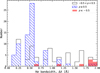 |
Fig. 5 Distribution of bandpasses that maximise the correlation between Hα and Ca II. The black histogram shows the bandpass distribution for stars with a weak or no correlation coefficient (−0.5 < ρ < 0.5), the blue hatched histogram shows stars with strong positive correlations (ρ ≥ 0.5), and the red histogram shows stars with strong negative correlations (ρ ≤ −0.5). |
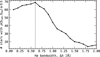 |
Fig. 6 Number of stars with a correlation coefficient between Ca II and Hα greater than 0.5 (strong positive correlation) for different band-widths. The vertical dashed line indicates the maximum at Δλ = 0.6 Å. |
6 Short-term correlations
After arriving at the conclusion that the bandwidth of 0.6 Å maximises the correlation between Ca II and Hα for long timescales, we are now interested in assessing what happens in the short term, more characteristic of the timescales of stellar rotation. Furthermore, we are interested in seeing the behaviour of the Hα index, using wide or narrow bandwidths, when the stars are at the maximum and minimum of their activity cycles. To achieve this, we need to identify the epochs of activity minima and maxima in the time series and then calculate the correlation coefficient between the SCa II and SHα06, and the SCa II and SHα16 indices for these epochs. Main sequence FGK stars have rotation periods that range from <1 day to around 60–70 days, depending on their ages (McQuillan et al. 2014), while the magnetic cycles of these types of stars are of the orders of years to decades (Baliunas et al. 1995). We therefore need to select the maxima and minima epochs with timespans long enough to be able to cover the range of rotation periods of these stars, while being short enough to isolate the maxima of activity from the minima and to exclude the effect of long-term variations associated with magnetic cycles. The maxima and minima epochs were identified using the following methodology. First, we grouped the SCa II, SHα06, and SHα16 time series into a grid of 30 day steps. This value, close to the higher envelope of the rotation periods of FGK dwarfs (McQuillan et al. 2014, Fig. 1), was enough to cover most of the rotation periods in just one grid step. Each epoch was defined as a group of points surrounded by empty steps, so that, for example, two (30-day) consecutive steps surrounded by two empty (30-day) steps would constitute an epoch (with a 60-day step); only epochs with at least seven observations were considered to ensure we had minimum points to calculate the correlation coefficients. The epoch with the highest SCa II mean value was the epoch at the activity maximum, while the epoch with the lowest SCa II mean was the activity minimum. To ensure that the activity levels of the maximum and minimum epochs were well separated in activity level, we imposed that the difference between the means of each epoch was at least two times the average standard deviations of the two epochs:  . This resulted in 103 stars with well-separated epochs of activity maxima and minima. The timespans obtained for the maxima and minima epochs range between 6 and 238 days, with the median at 88 days. The SCa II time series for these stars, with the maxima and minima identified with red and blue points, respectively, are provided in Appendix B. After completing this selection process, we calculated the Spearman correlation coefficients between SCa II and SHα06, and SCa II and SHα16, and their respective p-values, for the maximum and minimum epochs of each star. The correlation coefficients along with p-values and mean and standard deviation of SCa II for the full sample (before applying point 5 of the above selection) are provided in Table C.3. Contrary to the case of the long-term correlations in Sect. 5, not all stars with |ρ| > 0.5 have p-values ≤ 10−3, which means that there are cases of strong correlations that are not statistically significant. This is probably a consequence of the reduced number of data points in these datasets when compared to the full datasets used in the long-term analysis.
Figure 8 presents the distribution of the correlation coefficients between SCa II and SHα at maxima (red line) and minima (dashed black line) for the cases of SHα06 (top panel) and SHα16 (bottom panel). The correlations with significant coefficients (p-value ≤ 10−3) are represented by the filled red histograms for the activity maxima and black-hatched histograms for the activity minima. The first thing to note is that the only cases of significant correlations, for both SHα06 and SHα16, are positive correlations with ρ close to or above 0.5. There are more cases of strong positive correlations (ρ ≥ 0.5) at the maximum than at the minimum of activity for both Hα indices, while there are more cases of strong negative correlations (ρ ≤ −0.5) at the minimum than at the maximum. Similarly to the long-term case, using the 0.6 Å bandwidth in Hα maximises the number of stars with strong positive correlation with the calcium lines, both for epochs at the maximum and minimum of activity. However, the number of significant p-values (≤10−3) at minimum (black-hatched histogram) is the same for the two indices.
Out of the 103 stars analysed, 50 (49%) show strong positive correlations between SCa II and SHα06 at activity maximum (15, 15%, having a p-value ≤ 10−3), while 23 (22%) have strong positive correlation at activity minimum (1, 1%, having a p-value < 10−3). There are no cases of significant negative correlations between SCa II and SHα06 at the maximum or minimum of activity. In comparison, when using SHα16, only 26 stars (25%) showed strong positive correlations (7, 7%, with a p-value ≤ 10−3) at activity maximum and 14 (14%) at activity minimum (1, 1%, with a p-value ≤ 10−3). The figure also shows that, at these shorter timescales, there are more cases of anti-correlations, both at the minimum and the maximum of activity for SHα06. We should note, however, that we are using considerably fewer data points to compute the correlations at short timescales, and this will influence the significance of the correlation coefficients, as demonstrated by the reduced number of cases with p-values below 10−3.
An example of the improvement of using the narrower bandwidth also at short timescales is given in Fig. 9, where we show the rotational modulation of the K dwarf HD 109200 as measured by SCa II (upper panel), SHα06 (middle panel), and SHα16 (lower panel), selected at a region close to the activity cycle maximum. As can be observed, the SHα06 signal closely follows the modulation observed in SCa II while the signal from SHα16 appears to degrade the modulation signal. This has implications for the detection of rotation periods of stars when using the Hα time series. If a wide Hα bandwidth is used, the rotational modulation could be degraded, diminishing the significance of the signal. In the case of RV analysis in the context of exoplanet detection, this could increase the rate of false positives, by failing to identify activity signals, their harmonics, and aliases.
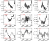 |
Fig. 7 SCa II, SHα16, and SHα06 for HD 215152 (top panels), HD 20003 (middle panels), and HD 7199 (lower panels). |
7 Discussion
7.1 Trends with effective temperature, metallicity, and activity level
Although using a 0.6 Å bandwidth maximises the correlation between SCa II and S Hα, still about half of the stars show weak or no correlation. To understand why, we searched for clues by analysing the correlation coefficient between SCa II, SHα06, and SHα16 against the stellar parameters effective temperature, metallicity, and the activity level measured by log R′HK.
The top panel of Fig. 10 shows that there is no trend of the SCa II-SHα16 correlation (red squares) with effective temperature. This was also observed by Gomes da Silva et al. (2014) and Meunier et al. (2022) using a 1.6 Å Hα bandpass. However, when using SHα06 as the Hα index (black circles), we see that almost all K dwarfs (Teff < 5250 K) have strong positive correlations, while hotter F and G stars have strong positive (ρ ≥ 0.5), weak or no correlations (−0.5 ≤ ρ ≤ 0.5), and strong negative correlations (ρ ≤ −0.5).
In the middle panel, when using SHα16 (red squares), there is a tendency for the strong negative correlations (ρ ≤ −0.5) to be present at higher metallicity values, as was previously observed by Gomes da Silva et al. (2014). This trend disappears when using SHα06 (black circles), meaning that the correlation between SCa II and SHα06 is not related to the metal content of stars.
The impact of the CaII activity level on the SCa II-SHα16 correlation was already observed for FGK dwarfs by Gomes da Silva et al. (2014) and Meunier et al. (2022), and for M dwarfs by Walkowicz & Hawley (2009) and Gomes da Silva et al. (2011), where more active stars have a tendency to show strong positive correlations, while negative and weak or no correlations appear preferably for inactive stars. The bottom panel shows this tendency is present when using SHα16 (red squares). However, for a narrow bandpass on Hα (black circles), we find that the strong positive correlations can be present for a greater number of inactive stars, including those with logR′HKlevels below −5.0 dex. There are also no strong negative correlations when using SHα06 (except one possible outlier). The correlation between SCa II and SHα06 seems to be independent of the activity level of the stars.
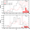 |
Fig. 8 Distribution of the correlation coefficient between SCa II and SHα06 (upper panel), and between SCa II and SHα16 (lower panel). The red histograms are the coefficients for epochs at the maximum of activity (p-value ≤ 10−3, filled red) while the black histograms are the coefficients for epochs at minimum (p-value ≤ 10−3, hatched black). |
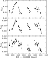 |
Fig. 9 Rotational modulation near the activity cycle maximum of HD 109200 measured by the SCa II (upper panel), SHα06 (middle panel), and SHα16 (lower panel) activity indices. |
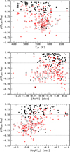 |
Fig. 10 Spearman correlation coefficient between SCa II and SHα06 (black circles), and between SCa II and SHα16 (red squares), against effective temperature (top panel), metallicity (middle panel), and median logR′HK activity level (bottom panel). Horizontal dotted lines mark the thresholds for strong correlations at ρ = 0.5 and −0.5. Filled markers are significant correlations with p-value < 10−3. |
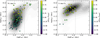 |
Fig. 11 Stellar activity variability measured as |

7.2 The effect of activity variability
Gomes da "R18"Silva et al. (2021) studied the chromospheric activity of FGK stars and found that the vast majority of the K dwarfs in their sample (including stars and observations used here) have high log R′HK variability, even though they are considered inactive, with log R′HK < −4.75 dex. The authors also observed that F and G inactive dwarfs can have both low and high variability, and that FGK dwarfs with activity levels above around −4.8 dex tend to have high variability. We therefore suspect that the explanation for the lack of stars with weak or no correlation for higher activity levels (log R′HK > −4.8 dex) and for K dwarfs (Teff < 5250 K) might be the same: high activity variability. To test this, we plotted the activity variability-level diagram with a 2D density map from the Gomes da Silva et al. (2021) catalogue using just main sequence stars, and overplotted the stars from this sample using squares for stars with strong positive correlation (ρ ≥ 0.5) and inverted triangles for stars with weak or no, or negative correlation (ρ < 0.5), coloured after their ρ value, as shown in Fig. 11. As we can see, the majority of the stars with strong positive correlation have high activity variability (with  dex), while the stars with weak or no correlation have low variability. Furthermore, activity level is not a main factor for strong positive correlations between SCa II and SHα06, since they are present in both inactive and active stars, as can also be observed in thge lower panel of Fig. 10.
Figure 11 also shows why we previously found that almost all K dwarfs have strong positive correlations (right panel) while some FG dwarfs show weak or no correlations (left panel): almost all K dwarfs have high activity variability, while F and G dwarfs show a greater range in variability that reach lower amplitudes. This shows that, instead of the activity level, the Ca II variability (here measured by the logarithm of the dispersion of R5 = 105 × R′HK) is one of the main contributions to the correlation between Ca II and SHα06.
7.3 The Hα wings
In the previous sections, we showed that the inclusion of flux from the Hα wings in the SHα index increases the number of strong negative correlations between SCa II and SHα, and deteriorates the activity signals, especially for stars with lower activity levels and a higher metal content. To inspect the behaviour of the Hα wings with SCa II activity, we constructed a new index, SHαW, using the flux of Hα, considering a bandpass with limits between those of 1.6 and 0.6 Å. The Spearman correlation coefficient between SCa II and SHαW, and the corresponding p-values were calculated according to the methodology described in Sect. 4.
Most of the significant correlations between SHαW and SCa II are negative, and these are present mainly for inactive stars with log R′HKbelow around −4.9 dex and stars with higher metallicity (Fig. A.1). This behaviour explains the anti-correlations between SCa II and SHα16 in inactive stars (Gomes da Silva et al. 2014; Meunier et al. 2022), and also the tendency for these to be present in higher-metallicity stars (Gomes da Silva et al. 2014). Interestingly, there are also a few stars with positive correlations between SCa II and SHαW, with ρ close to 0.5. These stars are typically G dwarfs with higher activity levels than the ones with negative correlations.
Figure A.2 shows the comparison between the time series of SCa II, SHα16, and SHαW for the same stars used before to exemplify the three different behaviours of the Hα index when compared to SCa II. For HD 215152 (upper panels), we saw in Fig. 7 that both the SHα06 and SHα16 indicators were positively correlated with SCa II, with SHα06 having a stronger correlation coefficient than SHα16. Here we see that the index based solely on the Hα wings flux has a very weak correlation with SCa II, which explains the SHα16 correlation being weaker than that of the core-based SHα06. In the case of HD 20003 (middle panels), there is a strong anti-correlation between SCa II and SHαW, which contributes to the mitigation of the strong positive correlation observed for SHα06 in Fig. 7 and results in a non-correlation for SHa16. In the case of HD 7199 (lower panels), the variation in flux with activity in the wings is higher (in negative values) than that of the core, as we saw in Fig. 4, turning the positive correlation between SCa II and SHα06 observed in Fig. 7 into a strong anti-correlation when the wings flux is added in SHα16.
Following these results, we can explain the correlation between S Hα and Hα based on the balance between the flux in the core and that of the wings. The flux in the Hα line core appears to be always (except for cases of low activity variability) positively correlated to that of the Ca II H&K lines. On the other hand, the flux in the Hα line wings has a tendency to be negatively correlated to that of the Ca II H&K lines, mainly in inactive and higher-metallicity stars. When the flux in the Hα line wings is included in the derivation of the SHα index, there will be strong negative correlations with the Ca II H&K lines for inactive and higher-metallicity stars when the variation in flux with activity in the wings is stronger than that of the Hα core. For the more active stars (log R′HK> −4.8 dex), the flux variation in the wings is irrelevant when compared to that of the core, producing a strong positive correlation.
Since the Ca II H&K lines are known to be well correlated with the presence of plages, this indicates that the core of the Hα line is following the same phenomena. The existence of strong (negative) correlations between the flux in the Hα line wings and Ca II H&K shows that the wings contain activity information. Meunier & Delfosse (2009) discussed the contributions of plages and filaments to the flux in the Hα line, showing that the contribution of plages would produce a positive correlation between the flux in Ca II and Hα, while filaments would contribute to a negative correlation, and thus the combination of plages and filaments could result in non-correlations or anti-correlations, depending on the plages’ and filaments’ filling factors, contrasts, and/or distributions (see also Meunier et al. 2022). It seems that, by separating the Hα line core from the line wings, we could be observing those behaviours separately, meaning that the flux in the Hα wings could be following the presence of filaments in the stellar disk. However, the identification of the structures responsible for the observed correlations is beyond the scope of the present work. Further investigations could be carried out by obtaining high-resolution spectra of different resolved activity structures in the Sun to analyse the Hα profile and compare the flux in the Hα line, measured with different bandwidths with the presence of specific activity features. This could be done, for example, with the future PoET Solar telescope (Santos et al., in prep.) to be installed at Paranal, Chile, and connected to the ESPRESSO spectrograph (Pepe et al. 2021).
8 Conclusions
In this work we have analysed the effect of varying the Hα bandwidth on the correlation between the SCa II and SHα activity indices using a sample of FGK stars observed with HARPS, with cadence and long enough timespans to detect rotation- and cycle-induced variability. We also compared the activity signals coming from long-term cycles and short-term rotation modulation using representative bandwidths: narrrow (0.6 Å) and wide (1.6 Å) bandpasses, and also a bandpass using just the line wings (1.6–0.6 Å).
While studying the correlations between SCa II and SHα for long and short timescales, in general we found similar results. However the statistical significance is stronger for the long-timescales case, probably due to the increased number of data points used.
The effect of changing the Hα bandwidth on the correlation between SCa II and SHα can be sumarised as follows:
Narrower bandwidths have a tendency for strong positive correlations with SCa II.
Wider bandwidths result in a great variety of correlations.
There are no cases where the correlation is stronger when using a wider bandwidth than using a narrower one.
Narrow bandwidths can convert some strong negative correlations observed with wider bands to strong positive correlations.
The bandwidth that maximises positive correlations with SCa II is 0.6 Å.
Previous works investigating the correlation between SCa II and SHα for FGK dwarfs using wide bandwidths, generally of 1.6 Å, have found that the correlation between SCa II and SHα depends on the activity level and metallicity, where for low activity levels and higher metallicity, there are non- and negative correlations, and for higher activity levels the correlations are strong positive (Gomes da Silva et al. 2014; Meunier et al. 2022). They also found that the correlation is not dependent on the effective temperature of stars. In this work we arrived at the same results. However, when analysing the correlations using a narrower bandpass of 0.6 Å, we found that most stars have strong positive correlations, independently of the activity level and metallicity. Furthermore, the cause fornon-correlations appears to be low activity variability.
We also analysed an index based on the flux of the Hα wings, and studied its correlation with SCa II. We found that the behaviour is similar to that of the Hα index with the wide 1.6 Å bandpass, but without strong positive correlations and with more cases of strong negative correlations.
Regarding the time series, we observed that both long-term activity cycle variations and short-term rotational modulated variations are better followed by SHα if using the narrower 0.6 Å bandwidth. This is more evidenced mainly for inactive and K dwarfs.
In conclusion, the correlation between SCa II and SHα16 depends on the balance between the flux variation with activity between the line core and line wings of Hα. While the Hα line core is positively correlated with S Ca II, the Hα wings show signs of following activity that is generally anti-correlated with the line core. This kind of Hα profile behaviour was previously observed for two solar analogues by Flores et al. (2016, 2018), and they suggested that the Hα index should be constructed taking the profile variations into account, instead of the integrated flux in the line. Here, we suggest a simple alternative solution by integrating the flux in a narrower bandwidth covering only the line core, which is able to achieve similar results.
Having demonstrated that the widely used 1.6 Å bandwidth on Hα degrades the quality of activity signals both at long and short timescales, we recommend the use of a narrower bandwidth, around 0.6 Å or between 0.25 ≥ ∆λ ≥ 0.75 Å, when calculating the Hα index. This will help to better identify both rotationally modulated and magnetic cycle activity signals, and to decrease false positives when identifying activity with the Hα for RV exoplanet searches.
Acknowledgements
This work was supported by FCT - Fundação para a Ciência e a Tecnologia through national funds and by FEDER through COMPETE2020 - Programa Operacional Competitividade e Internacionalização by these grants: UIDB/04434/2020 & UIDP/04434/2020; PTDC/FIS-AST/32113/2017 & POCI-01-0145-FEDER-032113; PTDC/FIS-AST/28953/2017 & POCI-01-0145-FEDER-028953.
Appendix A Plots of the SHαW analysis
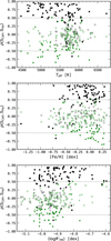 |
Fig. A.1 Spearman correlation coefficient between SCa II and SHα06 (black circles), and between SCa II and SHαW (green triangles) against the effective temperature (top panel), metallicity (middle panel), and median log R′HK. Horizontal dotted lines mark the thresholds for strong correlations at ρ = 0.5 and −0.5. Filled markers are significant correlations with p-value ≤ 10−3. |
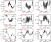 |
Fig. A.2 SCa II, SHα16, and SHαW for HD 215152 (top panels), HD 20003 (middle panels), and HD 7199 (lower panels). |
Appendix B Ca II time series and selection of maxima and minima
Figure B.1 shows the Ca II time series for the 103 stars used in the short-term analysis in § 6. Red and blue points mark the subsets used to calculate correlations at the higher and lower levels of activity, respectively.
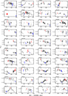 |
Fig. B.1 SCa II time series. Red points are the epoch at maximum, and blue points are the epoch at minimum. |
Appendix C Tables of stellar parameters and correlations
Stellar parameters for the sample.
Spearman correlation coefficients for the long-term dataset.
Spearman correlation coefficients for the short-term dataset.
References
- Baliunas, S. L., Donahue, R. A., Soon, W. H., et al. 1995, ApJ, 438, 269 [Google Scholar]
- Boisse, I., Moutou, C., Vidal-Madjar, A., et al. 2009, A&A, 495, 959 [NASA ADS] [CrossRef] [EDP Sciences] [Google Scholar]
- Boisse, I., Bouchy, F., Hébrard, G., et al. 2011, A&A, 528, A4 [NASA ADS] [CrossRef] [EDP Sciences] [Google Scholar]
- Bonfils, X., Mayor, M., Delfosse, X., et al. 2007, A&A, 474, 293 [NASA ADS] [CrossRef] [EDP Sciences] [Google Scholar]
- Cincunegui, C., Díaz, R. F., & Mauas, P. J. D. 2007, A&A, 469, 309 [NASA ADS] [CrossRef] [EDP Sciences] [Google Scholar]
- Dumusque, X., Udry, S., Lovis, C., Santos, N. C., & Monteiro, M. J. P. F. G. 2011, A&A, 525, A140 [NASA ADS] [CrossRef] [EDP Sciences] [Google Scholar]
- Dumusque, X., Pepe, F., Lovis, C., et al. 2012, Nature, 491, 207 [Google Scholar]
- Faria, J. P., Adibekyan, V., Amazo-Gómez, E. M., et al. 2020, A&A, 635, A13 [NASA ADS] [CrossRef] [EDP Sciences] [Google Scholar]
- Faria, J. P., Suárez Mascareño, A., Figueira, P., et al. 2022, A&A, 658, A115 [NASA ADS] [CrossRef] [EDP Sciences] [Google Scholar]
- Figueira, P., Santos, N. C., Pepe, F., Lovis, C., & Nardetto, N. 2013, A&A, 557, A93 [NASA ADS] [CrossRef] [EDP Sciences] [Google Scholar]
- Flores, M., González, J. F., Jaque Arancibia, M., Buccino, A., & Saffe, C. 2016, A&A, 589, A135 [NASA ADS] [CrossRef] [EDP Sciences] [Google Scholar]
- Flores, M., González, J. F., Jaque Arancibia, M., et al. 2018, A&A, 620, A34 [NASA ADS] [CrossRef] [EDP Sciences] [Google Scholar]
- Fontenla, J. M., Linsky, J. L., Witbrod, J., et al. 2016, ApJ, 830, 154 [Google Scholar]
- Gomes da Silva, J., Santos, N.C., Bonfils, X., et al. 2011, A&A, 534, A30 [NASA ADS] [CrossRef] [EDP Sciences] [Google Scholar]
- Gomes da Silva, J., Santos, N.C., Bonfils, X., et al. 2012, A&A, 541, A9 [NASA ADS] [CrossRef] [EDP Sciences] [Google Scholar]
- Gomes da Silva, J., Santos, N.C., Boisse, I., Dumusque, X., & Lovis, C. 2014, A&A, 566, A66 [NASA ADS] [CrossRef] [EDP Sciences] [Google Scholar]
- Gomes da Silva, J., Figueira, P., Santos, N., & Faria, J. 2018, J. Open Source Softw., 3, 667 [Google Scholar]
- Gomes da Silva, J., Santos, N.C., Adibekyan, V., et al. 2021, A&A, 646, A77 [NASA ADS] [CrossRef] [EDP Sciences] [Google Scholar]
- Kürster, M., Endl, M., Rouesnel, F., et al. 2003, A&A, 403, 1077 [NASA ADS] [CrossRef] [EDP Sciences] [Google Scholar]
- Livingston, W., Wallace, L., White, O. R., & Giampapa, M. S. 2007, ApJ, 657, 1137 [CrossRef] [Google Scholar]
- Lovis, C., Dumusque, X., Santos, N. C., et al. 2011, ArXiv e-prints [arXiv:1107.5325] [Google Scholar]
- Maldonado, J., Phillips, D. F., Dumusque, X., et al. 2019, A&A, 627, A118 [NASA ADS] [CrossRef] [EDP Sciences] [Google Scholar]
- Mauas, P. J. D., & Falchi, A. 1994, A&A, 281, 129 [NASA ADS] [Google Scholar]
- Mauas, P. J. D., & Falchi, A. 1996, A&A, 310, 245 [NASA ADS] [Google Scholar]
- Mauas, P. J. D., Falchi, A., Pasquini, L., & Pallavicini, R. 1997, A&A, 326, 249 [NASA ADS] [Google Scholar]
- Mayor, M., Pepe, F., Queloz, D., et al. 2003, The Messenger, 114, 20 [NASA ADS] [Google Scholar]
- McQuillan, A., Mazeh, T., & Aigrain, S. 2014, ApJS, 211, 24 [Google Scholar]
- Meunier, N., & Delfosse, X. 2009, A&A, 501, 1103 [NASA ADS] [CrossRef] [EDP Sciences] [Google Scholar]
- Meunier, N., Kretzschmar, M., Gravet, R., Mignon, L., & Delfosse, X. 2022, A&A, 658, A57 [NASA ADS] [CrossRef] [EDP Sciences] [Google Scholar]
- Noyes, R. W., Hartmann, L. W., Baliunas, S. L., Duncan, D. K., & Vaughan, A. H. 1984, ApJ, 279, 763 [Google Scholar]
- Pepe, F., Mayor, M., Rupprecht, G., et al. 2002, The Messenger, 110, 9 [NASA ADS] [Google Scholar]
- Pepe, F., Cristiani, S., Rebolo, R., et al. 2021, A&A, 645, A96 [NASA ADS] [CrossRef] [EDP Sciences] [Google Scholar]
- Queloz, D., Henry, G. W., Sivan, J. P., et al. 2001, A&A, 379, 279 [NASA ADS] [CrossRef] [EDP Sciences] [Google Scholar]
- Rajpaul, V., Aigrain, S., Osborne, M. A., Reece, S., & Roberts, S. 2015, MNRAS, 452, 2269 [Google Scholar]
- Rutten, R. G. M. 1984, A&A, 130, 353 [NASA ADS] [Google Scholar]
- Saar, S. H., & Donahue, R. A. 1997, ApJ, 485, 319 [Google Scholar]
- Santos, N. C., Mayor, M., Naef, D., et al. 2000, A&A, 361, 265 [NASA ADS] [Google Scholar]
- Santos, N. C., Gomes da Silva, J., Lovis, C., & Melo, C. 2010, A&A, 511, A54 [NASA ADS] [CrossRef] [EDP Sciences] [Google Scholar]
- Santos, N. C., Mortier, A., Faria, J. P., et al. 2014, A&A, 566, A35 [NASA ADS] [CrossRef] [EDP Sciences] [Google Scholar]
- Vaughan, A. H., & Preston, G. W. 1980, PASP, 92, 385 [Google Scholar]
- Vaughan, A. H., Preston, G. W., & Wilson, O. C. 1978, PASP, 90, 267 [Google Scholar]
- Walkowicz, L. M., & Hawley, S. L. 2009, AJ, 137, 3297 [NASA ADS] [CrossRef] [Google Scholar]
A python implementation of the algorithm is available at https://bitbucket.org/pedrofigueira/line-profile-indicators/src/master/.
As we see in Sect. 5.2, this is the bandwidth that maximises the correlation between SCa II and SHα.
Active stars are known to have strong positive correlations between SCa II and SHα.
All Tables
All Figures
|
Fig. 1 Distribution of the number of observations (upper panel) and timespan (lower panel) per star. |
| In the text | |
|
Fig. 2 Distribution of the effective temperature (left panel), metallicity (middle panel), and log R′HK activity level (right panel) for our sample. |
| In the text | |
|
Fig. 3 Effect of varying the Hα bandwidth in the correlation between Ca II and Hα coloured after activity level, measured as logR′HK. Upper panel: stars with strong positive (ρ ≥ 0.5) or negative (ρ ≤ −0.5) correlation with the SHα06 index. Stars marked with thick lines are examples used in Figs. 4, 7, and A.2, and the only case of negative correlation with SHα06 (HD 206998). Lower panel: stars with weak or no correlation (−0.5 < ρ < 0.5) with the SHα06 index. In both panels, as an indication, we mark the boundaries between strong and no correlation with horizontal dotted lines at ρ values of 0.5 and −0.5. |
| In the text | |
|
Fig. 4 Flux in the Hα line for different levels of activity. Upper panels: Hα line profiles of HD 215152 (left), HD 20003 (middle), and HD 7199 (right) at their maxima (red) and minima (blue) activity levels. Lower panels: difference between the fluxes at the maximum and minimum of activity for each star. Vertical lines show bandwidths of 2.0 Å (solid), 1.6 Å (dashed), and 0.6 Å (dotted). The numbers in the lower panels show the integrated flux difference in each region delimited by the vertical lines in red if positive and blue if negative. |
| In the text | |
|
Fig. 5 Distribution of bandpasses that maximise the correlation between Hα and Ca II. The black histogram shows the bandpass distribution for stars with a weak or no correlation coefficient (−0.5 < ρ < 0.5), the blue hatched histogram shows stars with strong positive correlations (ρ ≥ 0.5), and the red histogram shows stars with strong negative correlations (ρ ≤ −0.5). |
| In the text | |
|
Fig. 6 Number of stars with a correlation coefficient between Ca II and Hα greater than 0.5 (strong positive correlation) for different band-widths. The vertical dashed line indicates the maximum at Δλ = 0.6 Å. |
| In the text | |
|
Fig. 7 SCa II, SHα16, and SHα06 for HD 215152 (top panels), HD 20003 (middle panels), and HD 7199 (lower panels). |
| In the text | |
|
Fig. 8 Distribution of the correlation coefficient between SCa II and SHα06 (upper panel), and between SCa II and SHα16 (lower panel). The red histograms are the coefficients for epochs at the maximum of activity (p-value ≤ 10−3, filled red) while the black histograms are the coefficients for epochs at minimum (p-value ≤ 10−3, hatched black). |
| In the text | |
|
Fig. 9 Rotational modulation near the activity cycle maximum of HD 109200 measured by the SCa II (upper panel), SHα06 (middle panel), and SHα16 (lower panel) activity indices. |
| In the text | |
|
Fig. 10 Spearman correlation coefficient between SCa II and SHα06 (black circles), and between SCa II and SHα16 (red squares), against effective temperature (top panel), metallicity (middle panel), and median logR′HK activity level (bottom panel). Horizontal dotted lines mark the thresholds for strong correlations at ρ = 0.5 and −0.5. Filled markers are significant correlations with p-value < 10−3. |
| In the text | |
|
Fig. 11 Stellar activity variability measured as |
| In the text | |
|
Fig. A.1 Spearman correlation coefficient between SCa II and SHα06 (black circles), and between SCa II and SHαW (green triangles) against the effective temperature (top panel), metallicity (middle panel), and median log R′HK. Horizontal dotted lines mark the thresholds for strong correlations at ρ = 0.5 and −0.5. Filled markers are significant correlations with p-value ≤ 10−3. |
| In the text | |
|
Fig. A.2 SCa II, SHα16, and SHαW for HD 215152 (top panels), HD 20003 (middle panels), and HD 7199 (lower panels). |
| In the text | |
|
Fig. B.1 SCa II time series. Red points are the epoch at maximum, and blue points are the epoch at minimum. |
| In the text | |
Current usage metrics show cumulative count of Article Views (full-text article views including HTML views, PDF and ePub downloads, according to the available data) and Abstracts Views on Vision4Press platform.
Data correspond to usage on the plateform after 2015. The current usage metrics is available 48-96 hours after online publication and is updated daily on week days.
Initial download of the metrics may take a while.