| Issue |
A&A
Volume 668, December 2022
|
|
|---|---|---|
| Article Number | A181 | |
| Number of page(s) | 14 | |
| Section | Stellar structure and evolution | |
| DOI | https://doi.org/10.1051/0004-6361/202244468 | |
| Published online | 19 December 2022 | |
Lithium, masses, and kinematics of young Galactic dwarf and giant stars with extreme [α/Fe] ratios
1
Department of Astronomy, University of Geneva, Chemin Pegasi 51, 1290 Versoix, Switzerland
e-mail: This email address is being protected from spambots. You need JavaScript enabled to view it.
2
Institut d’Astrophysique de Paris, UMR7095 CNRS, Sorbonne Université, 98bis Bd. Arago, 75104 Paris, France
3
IRAP, CNRS UMR 5277 & Université de Toulouse, 14 avenue Édouard Belin, 31400 Toulouse, France
Received:
11
July
2022
Accepted:
25
September
2022
Abstract
Context. Recent spectroscopic explorations of large Galactic stellar samples stars have revealed the existence of red giants with [α/Fe] ratios that are anomalously high, given their relatively young ages.
Aims. We revisit the GALAH DR3 survey to look for both dwarf and giant stars with extreme [α/Fe] ratios, that is, the upper 1% in the [α/Fe]–[Fe/H] plane over the range in [Fe/H] between −1.1 and +0.4 dex. We refer to these outliers as “exαfe” stars.
Methods. We used the GALAH DR3 data along with their value-added catalog to trace the properties (chemical abundances, masses, ages, and kinematics) of the exαfe stars. We applied strict criteria to the quality of the determination of the stellar parameters, abundances, and age determinations to select our sample of single stars. We investigated the effects of secular stellar evolution and the magnitude limitations of the GALAH survey to understand the mass and metallicity distributions of the sample stars. Here, we also discuss the corresponding biases in previous studies of stars with high – albeit not extreme – [α/Fe] in other spectroscopic surveys.
Results. We find both dwarf and giant exαFe stars younger than 3 Gyr, which we refer to as “y-exαfe” stars. Dwarf y-exαFe stars exhibit lithium abundances similar to those of young [α/Fe]-normal dwarfs at the same age and [Fe/H]. In particular, the youngest and most massive stars of both populations exhibit the highest Li abundances, A(Li) ∼ 3.5 dex (i.e., a factor of 2 above the protosolar value), while cooler and older stars exhibit the same Li depletion patterns increasing with both decreasing mass and increasing age. In addition, the [Fe/H] and mass distributions of both the dwarf and giant y-exαFe stars do not differ from those of their [α/Fe]-normal counterparts found in the thin disk and they share the same kinematic properties, with lower eccentricities and velocities with respect to the local standard of rest than old stars of the thick disk.
Conclusions. We conclude that y-exαFe dwarf and giant stars are indeed young, their mass distribution shows no peculiarity, and they differ from young [α/Fe]-normal stars by their extreme [α/Fe] content only. However, their origins still remain unclear.
Key words: stars: abundances / stars: evolution / stars: kinematics and dynamics / Galaxy: evolution / Galaxy: stellar content
© S. Borisov et al. 2022
 Open Access article, published by EDP Sciences, under the terms of the Creative Commons Attribution License (https://creativecommons.org/licenses/by/4.0), which permits unrestricted use, distribution, and reproduction in any medium, provided the original work is properly cited.
This article is published in open access under the Subscribe-to-Open model. This email address is being protected from spambots. You need JavaScript enabled to view it. to support open access publication.
1. Introduction
One of the key questions in modern astrophysics concerns the formation and evolution of the Milky Way and its different substructures. Our Galaxy is a complex system consisting of different components (e.g., Helmi 2020; Gaia Collaboration 2022, and references therein), with the most prominent ones in the solar neighborhood being the thin and thick disks and the halo. The various aspects of the formation and subsequent dynamical and chemical evolution of each of those components, as well as the connections between them, are still poorly understood (e.g., Bland-Hawthorn & Gerhard 2016, and references therein).
Since the discovery of the thick disk (Gilmore & Reid 1983), it has been established that this component differs from the thin disk not only in terms of its spatial properties (i.e., it is more extended vertically), but also the kinematic properties (i.e., lower rotational velocity and higher velocity dispersion, e.g., Chiba & Beers 2000), as well as in the corresponding stellar ages, which are higher for the thick disk (e.g. Reddy et al. 2006). Regarding the chemical properties, the thick disk has lower metallicity (on average) and higher [α/Fe] ratios than the thin disk for the same metallicity (e.g., Prochaska et al. 2000; Mishenina et al. 2004). This latter property is understood as a natural consequence of the higher age of the thick disk which is supposed to evolve in a short timescale (a few Gy); this leaves less time to SN Ia to enrich the interstellar medium with their Fe-rich ejecta, in contrast to the thin disk which evolves on longer timescales of many Gyr. However, the observed co-existence of two clearly distinguished quasi-parallel [α/Fe] sequences in the same region of space – the solar cylinder – does not yet have a commonly accepted interpretation: very broadly, this could be due either to some specific dynamical event, such as an early merger or “quenching” of star formation followed by secondary infall (Larson et al. 1980) or by secular disk evolution (e.g., Schönrich & Binney 2009; Loebman et al. 2011).
Adibekyan et al. (2011) found that high [α/Fe] dwarf stars appear separated into two families with a gap in the distributions of both [α/Fe] and metallicity at [α/Fe] ∼ 0.17 and [Fe/H] ∼ − 0.2). They found that both the metal-poor high-[α/Fe] stars (thick disk) and the metal-rich high-[α/Fe] stars are, on average, older than the chemically defined thin disk stars (low-[α/Fe] stars). They adopted the term “hαmr” to characterize high-[α/Fe] and metal-rich stars, which were found to have kinematics and orbits similar to the thin disk stars, but are older by a few Gyr, that is, they have ages intermediate between those of the thick and thin disks.
The use of large spectroscopic surveys, such as RAVE (Steinmetz et al. 2006, 2020), APOGEE (Majewski et al. 2017), LAMOST (Zhao et al. 2012; Luo et al. 2015), GALAH (Buder et al. 2021) or Gaia-ESO survey (Gilmore et al. 2012), have provided a wealth of opportunities in the fields of stellar physics and Galactic archaeology over the past few years. A number of recent studies have reported young giant stars with [α/Fe] values higher than predicted by standard chemical evolution models of the Milky Way (Chiappini et al. 2015; Martig et al. 2015; Silva Aguirre et al. 2018; Wu et al. 2018; Miglio et al. 2021; Zhang et al. 2021). Using CoRot (Baglin et al. 2006) and APOGEE data, Chiappini et al. (2015) found that these stars have a lower iron-peak element content than the rest of the sample and are more abundant towards the inner Galactic disk regions. Their tentative interpretation of these observations is that these stars were formed close to the end of the Galactic bar, that is, near corotation. This is a region where gas can be kept inert for longer times than in other regions that are more frequently shocked by the passage of spiral arms and where the mass return from older inner-disk stellar generations is expected to be highest (according to an inside-out disk-formation scenario), which additionally dilutes the in-situ gas. On the other hand, using LAMOST and Gaia DR2, Zhang et al. (2021) found similar red giant stars with high masses and sharing the same kinematics as the high-[α/Fe] old stellar population in the Galactic thick disk. According to Zhang et al. (2021), these stars mimic “young” single stars, but they actually belong to an intrinsic old stellar population, as the thick disk. Similarly, Miglio et al. (2021), studying red-giant stars with exquisite asteroseismic (Kepler), spectroscopic (APOGEE), and astrometric (Gaia) data find that massive (M ≥ 1.1 M⊙) [α/Fe]-rich stars are a fraction of ∼5% on the RGB, and significantly higher in the red clump, apparently supporting the scenario according to which most of these stars had undergone an interaction with a companion.
In this paper, we focus on the uppermost envelope (the upper 1%) of the [α/Fe] values of dwarf stars of GALAH, independently of their metallicity. We show that some of them have unexpectedly young ages. We propose to use the term exαFe for those stars with extremely high [α/Fe] values, and y-exαFe for the youngest of them (i.e., with ages below 3 Gyr, see below). We begin in Sect. 2 with an overview of our dwarf sample and the relevant indicators of age for y-exαFe stars. In Sect. 3, we describe the young [α/Fe]-rich stars problem for giants and compare the results obtained for giants with the use of the LAMOST survey and other selection criteria. Finally, we summarize our results and present our conclusions in Sect. 4.
2. Extreme [α/Fe]-rich (exαFe) dwarf stars
2.1. Selection of the dwarf sample(s)
The selection criteria for the dwarf samples are described below and summarized in Table 1. The locations of the selected stars in the Kiel diagram are shown in Fig. 1.
 |
Fig. 1. Kiel diagram for the dwarf and giant stars selected from GALAH DR3. Upper panel: number density plot showing the positions of α-normal stars of the main samples of dwarfs and giants. Squares show the positions of extreme [α/Fe]-rich (exαFe, see Sect. 2.2.1) dwarf stars: y-exαFe (age ≤ 3 Gyr) and older exαFe are shown by blue and red squares, respectively. We keep the same notations, but in circles, for giants. Bottom panel: same details, but for stars in the additional sample (open symbols). |
Selection criteria applied to build the different sub-samples of dwarfs we consider in this work.
2.1.1. Stellar parameters and abundances
We selected dwarf stars with −1.1 ≤ [Fe/H] ≤ 0.4 dex and in a wide [α/Fe] range (−0.15 ≤ [α/Fe] ≤ 0.7) with ages and masses from the third data release of the GALAH survey, namely, the value-added catalog (Buder et al. 2021, VAC). We eliminated the binaries and pre-main sequence stars (flag_sp=0). We selected stars with log g ≥ 3.5 when Teff ≥ 5500 K and log g ≥ 3.8 when Teff < 5500 K, as shown in Fig. 1; thus focusing our attention on dwarfs and possible subgiants to avoid evolved stars with Li abundances modified by the first dredge-up (e.g., Charbonnel et al. 2020; Martell et al. 2021). We applied strict quality criteria to assure a reliable determination of the stellar parameters (Teff, log g) and of the values of [Fe/H] and [α/Fe] (i.e., we use the following flags: flag_sp=0, flag_fe_h=0, flag_alpha_fe=0, and S/N per pixel ≥ 30).
The [α/Fe] values reported in the GALAH DR3 catalog are calculated as an error-weighted combination of selected individual lines of Mg, Si, Ca, and Ti (nine lines in total for all the four elements). In this combination, the abundances of three elements are non-LTE: Mg (Osorio et al. 2015), Si (Amarsi & Asplund 2017), and Ca (Osorio et al. 2019). If one or more of the selected lines “fail” the quality test, the estimation is a combination of the rest, but no information is given on the actual number of lines and the actual combination of Mg, Si, Ca, and Ti that were used to compute the [α/Fe] values for individual stars. Since we place special emphasis on the content of α-elements in young stars, we selected those objects with σ[α/Fe] ≤ 0.05 dex.
Finally, to study the Li behavior of the dwarf stars, we selected among them those with reliable [Li/Fe] (flag_li_fe=0 in VAC). We computed A(Li) = [Li/Fe]+[Fe/H]+A(Li)⊙ with A(Li)⊙ = 0.96 dex (Wang et al. 2021) and considered only those objects with A(Li) ≥ 0 dex.
2.1.2. Ages, masses, and corresponding uncertainties
In this work, we consider the ages and masses provided in GALAH VAC that were obtained with the Bayesian stellar parameter estimation code BSTEP (Sharma et al. 2018) using PARSEC+COLIBRI isochrones from Marigo et al. (2017). However, to better handle the uncertainties on these two quantities, we independently computed the ages and masses of the dwarf sample with the SPInS tool (Lebreton & Reese 2020) which relies on pre-computed stellar models (we used the solar-scaled BaSTI evolutionary tracks from Pietrinferni et al. 2004, 2006) and MCMC approach. The input observables used for the stars are Teff, luminosity L, log g, and [M/H] (we computed [M/H] from [Fe/H] and [α/Fe] using the formula from Salaris & Cassisi 2005). We computed the luminosity using Gaia EDR3 G-band photometry based on the formula  , where
  (Prša et al. 2016), BCG is the bolometric correction computed according to Andrae et al. (2018), d is the distance (Bailer-Jones et al. 2021), and AG is interstellar extinction. The mean relative difference between “GALAH ages” and “SPInS ages” is 32%, with the mean relative uncertainties σ on age of ∼30% and ∼37% from GALAH and SPInS, respectively. While the age uncertainties are quite large, which still remains one of the problems in stellar astrophysics, this comparison confirms that the vast majority of the stars that are young according to GALAH are indeed young in terms of single-stellar-evolution scenario – independently of the methods based on isochrones or evolutionary tracks.
In addition to the criteria described in Sect. 2.1.1, we only kept stars with relative uncertainties of age lower than its mean uncertainty (σage/age ≤ 30%) from VAC for what we consider as our main sample. This is the sample with the strictest criteria for all the stellar properties that we discuss in this paper. On the other hand, isochrone-based age determination is (per se) less accurate in some areas of the Hertzsprung-Russel diagram (or Kiel diagram), in particular near the zero age main sequence (ZAMS) for the dwarfs with the lowest masses that exhibit both the longest MS lifetimes and the shortest MS “paths” in the HRD. Thus, we also included a separate sample with stars with higher age uncertainties (σage/age > 30%). This “additional” sample contains mostly low-mass stars that lie close to the ZAMS and which are nearly absent in the sample (Fig. 1). In both the main and additional samples, we eliminate stars with ages < 0.5 Gyr and > 13 Gyr because the age distribution shows sharp peaks in these ranges, which is probably caused by the convergence of the method to the lower and upper limits of the stellar evolution models grid. The resulting main and additional samples contain 105 297 and 33 947 dwarf stars, respectively. The main and additional “Li-sub-samples” (stars with measured Li abundances) contain 55 508 and 11 326 dwarf stars, respectively (Table 1).
Regarding the stellar masses, we put no constraint on the mass uncertainty because the mean mass uncertainties for our dwarf sample is low (∼4%).
2.2. Exαfe dwarfs and their properties
2.2.1. Defining exαFe dwarfs as outliers in the [α/Fe]-[Fe/H] plane
The positions of the dwarf stars in the [α/Fe] vs. [Fe/H] diagram are shown in Fig. 2 for both the main and additional samples. Here, we follow Buder et al. (2021), who refer to it as the Tinsley–Wallerstein diagram.
 |
Fig. 2. Properties of the dwarf stars of the main and additional samples (left and right columns, respectively; see details in Table 1) in the Tinsley–Wallerstein diagram. The solid curve separates the top 1% of stars in each of the 10 metallicity bins from the remaining 99% (exαFe and [α/Fe]-normal stars, respectively), whereas the dashed curve is the median (50% of stars above and below it). From top to bottom: ages, masses, and Li abundances are color-coded, with the color of the background indicating the mean value of the property in bins of size 0.0125 dex in [Fe/H] and 0.0094 dex in [α/Fe]. Individual stars with age ≤3 Gyr and A(Li) ≥ 2.65 dex are also indicated by big and small points for stars above and below the top 1% curve, respectively. |
We selected extreme [α/Fe]-rich (exαFe) stars as outliers with the highest [α/Fe] values in the main and additional samples described in the previous section. We split the considered [Fe/H] range in ten bins of 0.15 dex width, keeping bins 1–4 at the same positions as in Charbonnel et al. (2021). In each metallicity bin, we compute the [α/Fe] value above which lie 1% of the stars of the main sample of this bin, namely, stars above the solid curve in Fig. 2 (we used the same curve to delineate exαFe both in case of the main and additional samples). In this way, we were able to keep the most “extreme” [α/Fe] stars of both samples, at more than 2σ (> 0.1 dex) from the median [α/Fe] value in each bin, which is indicated by the lower (dashed) curve (50%) in Fig. 2. The 1% curve can be approximated by [α/Fe] = −0.42 ⋅ [Fe/H] + 0.13 for [Fe/H] < 0 and −0.075 ⋅ [Fe/H] + 0.13 for [Fe/H] > 0. There are 1122 and 632 stars from (respectively) the main and additional samples in that region of the [α/Fe] vs. [Fe/H] plane (see Cols. 3 and 6 – exαFe and add-exαFe – in Table 1). In addition to their extreme [α/Fe] values, the properties of these stars differ considerably from those of the thick disk, as we argue in the following sections.
Since observational and analysis systematics could lead to a degeneracy between the determination of [Fe/H] and that of [α/Fe], we conducted a test to check if this could shift [α/Fe]-normal stars to the exαFe region in the Tinsley–Wallerstein diagram. We selected 584 GALAH DR3 stars from nine open clusters of various ages and metallicities using the same selection criteria as described in Sect. 2.1.1. For each cluster, we computed the mean [Fe/H] and [α/Fe] as well as the [Fe/H] and [α/Fe] deviation of individual member stars which should in principle share the same initial composition. Combining deviations of individuals of all the clusters, we derived the degeneracy trend in the Tinsley–Wallerstein diagram and found a slope of −0.36 ⋅ [Fe/H], which is lower than the approximate slope of the 1% curve of (−0.42 ⋅ [Fe/H]) mentioned in the previous paragraph. Hence, the degeneracy can possibly lead to a slight increase in [α/Fe] if [Fe/H] is underestimated. However, it cannot “shift” [α/Fe]-normal stars to the exαFe region above the 1% curve, unless the stars are already close to this limit.
2.2.2. Ages, masses, and Li content of exαFe dwarfs
In Fig. 2, we display some properties of the main and additional sample stars in Tinsley–Wallerstein diagram. In the top panels, we indicate the stellar ages, color-coded. We adopted bins of 0.0125 dex in [Fe/H] and 0.0094 dex in [α/Fe] and indicate the mean age of each bin. As expected, both on theoretical and observational grounds, the [α/Fe] values decrease with decreasing age of stars and increasing metallicity, ranging from more than ∼10 Gyr on the top left (thick disk) to less than a few Gyr in the bottom right (thin disk). [α/Fe] is a good proxy for age, at least for sub-solar [Fe/H] values. However, our exαFe sample defined in the previous section appears clearly to go against that trend, being dominated by young ages – and clearly younger than the bulk of the stars in most metallicity bins.
Among the 1122 exαFe stars of the main sample, ∼20% (280) are younger than 3 Gyr and we define them as y-exαFe stars (Young stars with EXtreme [α/Fe] ratio, see the fourth column y-exαFe of Table 1). The reasoning behind our choice to consider them to be a class apart can be clearly seen in Fig. 3 (top panel). While the [α/Fe]-normal sample displays a rather uniform age distribution (thin grey histogram), the exαFe sample (thick black histogram) displays two prominent regions: one at high ages (9–12 Gyr) which can, in principle, be identified with the thick disk; and another one at low ages, which is unexpected in view of their high [α/Fe] values. In contrast, the [α/Fe]-normal and exαFe samples are indistinguishable in their metallicity distributions (bottom panel in Fig. 3), both peaking at slightly sub-solar metallicity. These y-exαFe stars constitute the main topic of our work and we postpone a specific discussion of them in the next section, after surveying the other properties of our samples (mean properties in the aforementioned [α/Fe]–[Fe/H] bins).
 |
Fig. 3. Age (top) and [Fe/H] (bottom) distributions of the exαFe (thick black, scale on the left) and [α/Fe]-normal (thin grey, scale on the right) dwarf stars from the main (solid) and additional (dashed) samples. |
In the top right panel of Fig. 2, we display the ages of our add-exαFe sample. The trends in age are similar to the case shown in the top left panel for the main sample, although the oldest ages (> 10 Gyr) appear to be missing. As explained in Sect. 2.1.2, this is due to the higher age uncertainties (σage/age > 30%) of that additional sample, which contains mostly low-mass stars lying close to the ZAMS. This is clearly shown in the top panel of Fig. 3 (dashed histograms) for both the add-[α/Fe]-normal sample and the add-exαFe sample, the latter displaying an enhancement of its young population, as in the case of the main exαFe sample (solid histogram). The metallicity distributions of the add-[α/Fe]-normal sample and the add-exαFe sample are similar and peak at solar values (bottom panel of Fig. 3, dashed histograms). The shift in [Fe/H] between the main and additional samples is artificially induced by the lack of older, more metal-poor stars in the second one. When we combine both samples, the [Fe/H] distributions of the exαFe and [α/Fe]-normal dwarfs perfectly overlap with a peak at −0.1–0 dex.
The middle panels of Fig. 2 display the masses of the dwarf stars of our samples. The age trend of the top panels is now turned into a mass trend, with the older ages corresponding to lower masses, as expected: lower average masses are found at the lowest metallicities and higher [α/Fe] ratios. However, in the left middle panel, the exαFe sample (above the solid curve) again shows considerably higher average masses than the stars with lower [α/Fe] values immediately below the solid curve, in agreement with the young ages of the main exαFe stars in the top panel. Those stars are missing from the add-exαFe sample and, thus, the stars above the solid curve in the right middle panel are mostly of a low mass. There is a clear consistency between the picture emerging from the top and middle panels of Fig. 2.
In the bottom panels of Fig. 2, we display another key property of the stars of our samples, color-coding them according to their Li abundance. The interpretation of those panels is more difficult since their surface Li content depends on a combination of the two previous properties – age and mass – as well as their initial Li content, which is unknown because it depends on the chemical evolution of Li: in principle, the initial value of every star should be above the primordial one of A(Li)P = 2.65 (Pitrou et al. 2018). Additionally, substantial Li depletion may occur along the main sequence and even the pre-main sequence for low-mass stars (e.g. Magazzu et al. 1992; Deliyannis et al. 2000; Castro et al. 2016; Dumont et al. 2021; Jeffries et al. 2021). The bulk of our sample stars has mean values A(Li) ∼ 2.5 dex, lower than A(Li)P, in all the bins of the [α/Fe] vs. [Fe/H] diagram. For [α/Fe] > 0.2 and [Fe/H] < −0.4 (realm of thick disk) they become even lower, less than 1.5 dex.
The exαFe stars of the main sample (bottom left panel of Fig. 2) display higher mean values of Li than the stars of the thick disk. This is consistent with their higher average mass and lower average age (hence lower Li depletion), already discussed in the previous paragraphs. On the other hand, the exαFe stars in the add-sample (bottom right panel) display lower average Li values than the other stars of that sample, because they correspond to lower average masses, as shown in the middle right panel and discussed above. In fact, the stars of the thick disk in that panel (corresponding to [Fe/H] < −0.1 and [α/Fe] > 0.2) have no detectable Li values and are absent from this region of the diagram.
In summary, the exαFe stars of our main sample are, on average, younger and more massive than the remaining ones (i.e., the non-exαfe), and they are more (or at least as much) Li-rich. The exαFe stars of the additional sample are also younger on average, but less massive; for that reason, they are also Li-poorer than the remaining ones (the Li behavior in the exαFe stars will be discussed further in Sect. 2.3.2). As explained above, the differences in terms of stellar masses between the main and additional exαFe samples come directly from the isochrone age-dating method which precision depends on the positions of the stars in the HRD. The identification of these biases is of importance for compiling a relevant description and understanding of the exαFe population.
2.3. Young-exαFe dwarfs
In the previous section, we have identified a minority of stars – about one percent in the main and two percent in the additional samples of dwarf stars – with unexpectedly high values of [α/Fe] for their metallicity. We have shown that some of those stars – about 25% for the main and 40% for the additional sample – are also young, younger than 3 Gyr (y-exαFe stars). The existence of a population of “young” red giant stars with “high [α/Fe]” has already been reported with APOGEE data (e.g., Chiappini et al. 2015; Martig et al. 2015; Anders et al. 2017; Silva Aguirre et al. 2018) and LAMOST (Zhang et al. 2021), albeit with very different limits regarding [α/Fe] and age than adopted here (Sect. 3). It has been argued that the properties of those stars should be interpreted by considering that they are, in fact, old stars with high [α/Fe] which have merged recently: this would explain their higher than average mass reported by previous studies, and make them appear younger (e.g., Zhang et al. 2021; Miglio et al. 2021).
In the following, we further explore the various properties of the y-exαFe dwarf population, namely, mass, Li abundance and kinematics, and we show that the interpretation in terms of mergers cannot hold. We also discuss the case of y-exαFe giants in Sect. 3.
2.3.1. Ages, metallicities, and masses
We overplot in each panel of Fig. 2 the exαFe stars with young ages (< 3 Gyr) and Li abundances higher than the primordial BBN value of A(Li)P = 2.65 (Pitrou et al. 2018). They are displayed as individual large dots (and not as average values for each pixel, as was done for the other stars) in the top part of each panel (the exαFe region above the solid curve). For the purposes of comparison, we also plotted as small dots the individual values for all the stars younger than 3 Gyr of our main and additional samples in all the panels. For all stars and panels, the color-coding is the same as adopted in the previous section and indicated on the vertical bars on the right.
In all the panels, the large majority of young stars are positioned where they are expected to be, namely, the thin disk, around −0.3 < [Fe/H] < 0.2 dex and −0.1 < [α/Fe] < 0.1 dex (small dots). These stars have also high Li content, as expected, and higher mass than the average of their pixel. Among the exαFe we also find similar stars which at the same time have young age, high [α/Fe] and high Li (large dots).
The mass distribution of the y-exαFe dwarf stars appears in the top panels of Fig. 4, both for those of the main sample (solid histograms) and of the additional sample (dotted). To interpret these figures, it is important to keep in mind that the GALAH survey is magnitude-limited (see Sect. 2.1 and Fig. 4a in Buder et al. 2021): on the one hand, it contains almost no stars brighter than V = 9m, implying that massive (luminous) dwarfs stars are absent at small distances. On the other hand, the sample has also a lower luminosity limit – the V-band distribution drops very steeply at V = 14m – and it contains only ∼1% of dwarf stars that are fainter. As a result, the relative number of low-mass dwarfs (both exαFe and [α/Fe]-normal) decreases at larger distances. Indeed, the additional y-exαFe sample is composed of small mass stars (< 1 M⊙), which dominate the volume close to the Sun (distance d < 200 pc, top left) because of their large number in the initial mass function. The main y-exαFe sample is composed of rather massive stars (M > 1.2 M⊙), which are less numerous because of the IMF; however, they are visible at larger distances and dominate completely in the distance range 500 < d (pc) < 2500. As a result of the selection criteria we used, as well as the characteristics of the GALAH survey, the total sample of y-exαFe stars (main plus additional for d < 2500 pc) shows a bimodal behavior, as seen in the top right panel. We checked that this bimodality also appears for the exαFe sample, albeit to a smaller degree (middle panels in Fig. 4), and with a shift of the high mass peak due to age limit considered as more massive stars have shorter MS lifetimes. The bimodality persists at still lower level for the [α/Fe]-normal stars (bottom panels). It is thus an artificial pattern that results from the adopted selection criteria applied to a magnitude-limited survey.
 |
Fig. 4. Mass distribution of y-exαFe (top), all exαFe (middle) and [α/Fe]-normal (bottom) stars. Nearby stars (distance D < 200 pc) are on the left panels and all stars up to 2500 pc on the right panels, for the main (solid) and additional (dotted) samples, respectively. |
The conclusion of this analysis asserts that: (a) the dwarf y-exαFe sample contains more massive and thus more luminous (and therefore seen to larger distances) than the older exαFe sample due to secular evolution effects (3 Gyr is approximately the main sequence lifetime of ∼1.2–1.6 M⊙ stars depending on their metallicity); and (b) once the selection biases discussed above are accounted for, y-exαFe dwarfs do not appear to have higher than average mass compare to their exαFe and [α/Fe]-normal counterparts.
2.3.2. Importance of Li for exαFe dwarfs
In Fig. 5, we display the Li abundance (when available) vs. Teff of the exαFe and [α/Fe]-normal dwarf stars (top and bottom panels, respectively) of the main and additional samples (left and right panels, respectively). The GALAH data are color-coded as a function of age. We note the similarities between the exαFe and the [α/Fe]-normal stars. First, the highest Li abundance is similar in both cases, with A(Li) ∼ 3.5, and it is found in the hottest (i.e., more massive) and youngest (y-exαFe and [α/Fe]-normal) stars. Second, the Li abundance decreases with increasing stellar age and decreasing effective temperature, with the latter being a proxy for the mass. This well-known behavior has long been observed in field and open cluster dwarfs (e.g., Zappala 1972; Sestito & Randich 2005). It is interpreted as the result of internal transport processes of chemicals which lead to differential photospheric Li depletion in stars of different masses and ages along the main sequence (and eventually already on the pre-main sequence for the lowest masses). Notably, Li depletion is minimal or eventually null in early-F and late A-type stars that exhibit the highest Li abundances close to the value they were born with (Charbonnel et al. 2021, and references therein).
 |
Fig. 5. Age color-coded A(Li) values as a function of Teff for exαfe and [α/Fe]-normal stars (upper and lower panels, respectively). Left and right columns are for the main and additional samples, respectively. |
We conclude from this analysis that: (1) the Li-abundance of the hottest y-exαFe dwarf stars is slightly (by a factor of (2)) above the proto-solar value of A(Li) = 3.26 dex and constitutes a strong argument for a young age; (2) the ages of the stars with the highest Li abundances, independently determined, are indeed low (less than a few Gyr); (3) Li depletion occurs similarly in exαFe and [α/Fe]-normal dwarfs; (4) the exαFe and [α/Fe]-normal populations were born with essentially the same maximum initial Li abundances.
The high Li content of the y-exαFe stars, which is similar to that of the young [α/Fe]-normal stars, makes it difficult to adopt the merger scenario as an explanation for their young age. The merger would indeed have to restore the exact original Li content of the two components, which would certainly require strong fine-tuning. In our opinion, this is a decisive argument against that scenario; however, it is not the only one. It is clear that old stars with high effective temperatures and high values of A(Li) are not generally observed, while the α-Li-richest stars (squares in the figure) also follow the general trend.
2.3.3. Kinematic properties
The kinematic properties of a sample of stars also provide interesting information on their origins. Here, we use the eccentricities and velocities of our GALAH dwarf sample, the latter being evaluated with respect to the local standard of rest ( ). These values are provided in the GALAH VAC and computed with the tool galpy (Bovy 2015). As a star evolves, these parameters are known to increase their average values: this process of dynamical heating is caused by interactions with different substructures of the Galaxy, such as spiral arms, giant molecular clouds, or the Galactic bar (e.g., Aumer et al. 2016; Mackereth et al. 2019; Almeida-Fernandes & Rocha-Pinto 2018).
As can be seen in Fig. 6, our y − exαFe stars have significantly lower eccentricities (top panel) and velocities with respect to VLSR (lower panel) than old stars of the thick disk. In both cases, the distributions look very similar to those for young [α/Fe]-normal stars which are found in the thin disk. Thus, the kinematic properties of the y − exαFe stars offer further evidence in favor of characterizing them based on a young age.
 |
Fig. 6. Distribution of eccentricities and velocities with respect to the local standard of rest VLSR (upper and bottom panels, respectively) for y-exαFe and young [α/Fe]-normal dwarfs stars (blue and grey histograms, respectively). The green histogram shows the distribution of old (age ≥ 8 Gyr) stars with [α/Fe] ≥ dex. The magenta histogram shows the distribution of 40 y-exαFe stars with A(Li) > A(Li)SBBN = 2.65. All the histograms are scaled to have the same height and we show the distributions for the main sample only for the purpose of better visibility. |
2.3.4. Discussion
Our findings in Sect. 2.3 for y-exαFe stars can be summarized as follows: about a quarter of the exαFe stars (high [α/Fe] outliers) of our main sample have ages evaluated to less than 3 Gyr; their young age is corroborated by other independent signatures, such as the presence of stars with higher mass (hence with shorter lifetimes) than in the rest of the sample and kinematic properties similar to that of young [α/Fe]-normal stars (low eccentricities and velocities). Last but not least, one fifth of them have high Li values, which behave in the same way as those of their [α/Fe]-normal counterparts. Taken all together, the above features suggest that those y-exαFe stars are indeed young. It seems difficult to accept the alternative idea of recent mergers of old, high [α/Fe] stars (Zhang et al. 2021; Miglio et al. 2021), since it would imply that such events somehow synthesize Li at the same level as in recently formed stars in the Galaxy.
In Fig. 7, we overplot our y-exαFe stars with high Li abundances (higher than A(Li)P = 2.65) on the [α/Fe] and [Fe/H] vs. age diagrams of our main dwarf sample. It can be seen that the youngest of them (less than 2 Gyr) have the highest Li content and that their Li decreases with increasing stellar age; both features are compatible with what is expected for a young stellar population. The metallicity of those stars is higher than [Fe/H] = −0.4, but their high [α/Fe] ratio is the only feature that does not fit to what is expected from a young stellar population.
 |
Fig. 7. Number density plots showing [α/Fe] and [Fe/H] (upper and bottom panels respectively) as a function of age for the main dwarf sample. Color-coded circles show the positions of the y-exαFe stars with A(Li) > 2.65 of the main and additional samples (filled and open circles, respectively) |
That high [α/Fe] ratio could, in principle, be attributed to recent episodes of star formation in the solar neighborhood. Indeed, Mor et al. (2019) analyzed Gaia DR2 data in combination with the Besançon Galaxy Model and found an imprint of a star formation burst ∼2–3 Gyr ago in the domain of the Galactic thin disk. In addition, Ruiz-Lara et al. (2020) analyzed Gaia DR2-observed color–magnitude diagrams to obtain a detailed star formation history of the ∼2 kpc bubble around the Sun, which reveals three conspicuous and narrow episodes of enhanced star formation. They date those episodes as having occurred 5.7, 1.9, and 1.0 Gyr ago, also suggesting that the timing of these episodes coincides with proposed Sgr pericenter passages.
The massive stars formed in those recent “mini-starbursts” eject soon after (within several Myr) their nucleosynthesis products, having an enhanced [α/Fe] ratio. If a new stellar generation is formed from those ejecta before they mix completely with the interstellar medium, stars with high [α/Fe] can be obtained having thin disk metallicities. Those formed locally or in the inner disk should have super-solar metallicities, while those in the outer disk sub-solar ones. Thus, the recent star formation episode should extend over a fairly large radial range of the thin disk in order to explain the broad range of [Fe/H] of the y-exαFe stars in the bottom panel of Fig. 7. In both cases, these stars could be transported to the solar neighborhood by radial migration in the thin disk, being simultaneously young, relatively massive, with thin disk kinematics and high [α/Fe].
However, the Li content of the exαFe stars should be then depleted, since massive star ejecta are expected, in principle, to be Li poor, unless neutrino-induced nucleosynthesis manages to produce large amounts of Li during the explosion (Woosley et al. 1990). The (presently) poorly known neutrino spectra are the main problem in evaluating the contribution of massive stars to Li production in the Galaxy. A thorough assessment of all Li sources during Galactic evolution was made in Prantzos (2012), who evaluated the maximum possible contribution of CCSN to 20% and, more realistically, down to just a few percent. However, even in the case of such a recent star formation “burst”, it would be surprising to have Li at the same level as the one observed in our y-exαFe stars, which corresponds to standard Galactic evolution (see discussion in Sect. 2.3.2). In fact, barring the case of short-lived Li sources, the Li abundance of the Galactic gas is expected to decrease in that case (although this is quantitatively difficult to estimate as it depends on many assumptions), in contrast to what is observed in the stars of our y-exαFe sample.
3. Exαfe and y-exαFe red giants
We now turn to exαFe and y-exαFe red giants. We applied the same selection criteria as for the dwarfs presented above and so, we discuss the implications of these differences on the conclusions of previous studies of so-called young [α/Fe]-high red giants.
3.1. Sample selection
We selected giant stars from GALAH DR3 applying the same criteria as for the dwarf main and additional samples, except for the log g and Teff domains (Fig. 1). The age determination through the isochrone-based method leads to higher uncertainties for giant than for dwarf stars, especially in the low-mass range (≤2 M⊙) where evolution tracks are close from the Hayashi limit up to the RGB tip. As a result, we have about three times more giant stars in the additional sample than in the main one (we had the inverse ratio for the dwarfs), with a large fraction in the low-mass range. We identified the exαFe giants as those above the 1% curve that is re-computed for the entire giant sample (Fig. 8). Finally, we did not consider Li as an age indicator since its abundance is strongly affected in red giants during the first dredge-up episode and later above the RGB bump (Charbonnel et al. 2020, and references therein). The information about the resulting main and additional samples is summarized in Table 2, and Fig. 1 shows the positions of the selected giants in the Kiel diagram.
 |
Fig. 8. Properties of the giants of the main and additional samples (left and right columns, respectively) in the Tinsley–Wallerstein diagram. Small squares represent bins with more than five stars. Blue points show the positions of young (< 3 Gyr) stars. |
Selection criteria applied to build the different sub-samples of giants from the GALAH catalog.
3.2. Properties of the exαFe and y − exαFe giants
The ages and masses of the selected giant stars are color-coded in the Tinsley–Wallerstein diagram in Fig. 8, and we show the age and [Fe/H] distributions of the exαFe and [α/Fe]-normal stars in Fig. 9 (compare respectively to Figs. 2 and 3 for the dwarfs). As in the case of the dwarfs, the [Fe/H] distributions of the exαFe and [α/Fe]-normal giants are very similar, and we retrieve the global decrease of [α/Fe] with decreasing stellar age for the [α/Fe]-normal giants. The age distribution of the exαFe giants from the main sample is similar to that of the exαFe dwarfs, albeit with a larger fraction being younger than 3 Gyr (compare to Fig. 3). The additional sample also contains y-exαFe giants, although it is dominated by old low-mass stars whose evolution tracks along the RGB make the age determination more uncertain. Finally, y-exαFe giants are found in all metallicity bins, both in the main and additional samples, as observed in the dwarf sample.
 |
Fig. 9. Age (top) and [Fe/H] (bottom) distributions of the exαFe (thick black, scale on the left) and [α/Fe]-normal (thin grey, scale on the right) giant stars from the main (solid) and additional (dashed) samples. |
We show in Fig. 10, the mass distributions (normalized numbers) of the old exαFe, y-exαFe, and young [α/Fe]-normal giants of the main sample; regarding the additional sample, we only show the mass distribution of the y-exαFe stars, for the purpose of clarity. We separated young and old stars assuming different age cuts, namely, 3 (as for the dwarfs), 4, and 6 Gyr, for a comparison with previous works (Sect. 3.3). For the 3 Gyr case, two peaks appear in the mass distribution of the main sample. On one hand, the peak located around ∼0.9–1.0 M⊙ corresponds to the exαFe giant stars with age > 3 Gyr that are climbing the RGB and whose age distributions peak around 10 Gyr (Fig. 9), which is approximately the main sequence lifetime of 0.9–1.0 M⊙ stars at [Fe/H] ∼ −0.5 dex. This explains why its position does not move when we increase the age cut. On the other hand, the mass distributions of the y-exαFe and young [α/Fe]-normal giants nicely overlap at 3 Gyr, with a peak around 1.9–2.0 M⊙ which contains stars that are presently close to or at the red clump (see Fig. 1). When we increase the age cut, this peak slightly moves towards lower masses, due to the dependence of the stellar lifetime with mass. An additional peak appears in the distribution of the young [α/Fe]-normal stars at intermediate masses (at ∼1.4 and 1.3 M⊙ for the age cuts of 4 and 6 Gyr, respectively, and barely visible at 1.5 M⊙ at 3 Gyr). It corresponds to stars whose main sequence lifetime is similar to or lower than the age cut, and which are climbing the RGB. Its position in mass thus decreases with increasing age limit. Because the age determination for giants in the corresponding mass domain is rather uncertain, this peak is much more pronounced for the y-exαFe from the additional than for those of the main sample (compare red full and dotted lines). Actually, when we consider the main and the additional samples together, the relative height of the RGB peak is much higher than that of the clump stars, and approximately at the same position in mass for the y-exαFe and the young [α/Fe]-normal giants.
 |
Fig. 10. Mass distribution of the giant stars assuming different age limits (3, 4, and 6 Gyr from bottom to top). Red histograms correspond to y-exαFe (i.e., younger than the age cut) giants of the main and additional samples (full and dotted respectively). The blue and black histograms correspond respectively to the young [α/Fe]-normal giants and to exαFe giants older than the cut (for these two cases we show only the distributions of the main sample stars). All the histograms are scaled to have the same height for the purpose of visibility, and the numbers on the left give the number of stars in each color-coded class of giants. |
Kinematics of giants (both eccentricities and VLSR) also tends to the fact that y-exαFe giants are indeed young (see Fig. 11). However, distributions of the kinematic parameters of y-exαFe and young [α/Fe]-normal are not absolutely similar, as the former exhibit lower eccentricities and VLSR than old exαFe.
 |
Fig. 11. Distribution of eccentricities (upper panel) and VLSR of the giants (same colors as in Fig. 10). |
We conclude from this analysis that: (1) the mass and metallicity distributions are the same for the y-exαFe and the young [α/Fe]-normal giants; (2) the positions of the peaks in masses found above for the giants stars reflect secular evolution effects, and do not result from an odd IMF; (3) their apparent respective heights depend on the criteria we impose on the precision of the age determination, but the “RGB peak” dominates over “clump peak” when we combine the main and the additional samples; (4) the kinematic parameters of y-exαFe giants and young [α/Fe]-normal giant stars are very similar, and they differ from those of exαFe and [α/Fe]-normal giants with age > 3 Gyr. This reinforces the conclusions we draw for the dwarf stars that the y-exαFe stars did not form through mergers but, rather, with an IMF similar to that of their [α/Fe]-normal counterparts.
3.3. Comparison to previous work
Previous studies of so-called “young, high [α/Fe]” red giant stars used different criteria both in terms of [α/Fe] and age, with 6 Gyr being usually assumed as the transition between young and old populations. The discovery of such stars in the Galactic disk in CoRoT-APOGEE (CoRoGEE) and Kepler-APOGEE (APOKASK) samples gave a new spin to the field, as asteroseismology has opened a new avenue to determine the age and mass of giants and to distinguish clump stars from RGB stars (e.g., Prantzos 2012; Chiappini et al. 2015; Martig et al. 2015; Anders et al. 2017; Silva Aguirre et al. 2018).
Zhang et al. (2021) expanded the statistics using LAMOST DR4 value-added catalog (Wu et al. 2019; Xiang et al. 2019), with ages and masses based on data-driven spectroscopic estimates (Teff, log g, C and N abundances) trained by a Kepler asteroseismic sample. They eliminated red clump stars and kept only RGB stars with 3000 < Teff < 5500 K, log g < 3.8, and −0.8 < [Fe/H] < 0.5 dex. They defined “high-α young giant stars” those with [α/Fe] higher than 0.18 dex independently of their [Fe/H] value, and with ages lower than 6 Gyr; they did not exclude stars based on age uncertainties. With their selection criteria, they obtained the peaks around 0.9–1.0 M⊙ for the “high-α old” RGB stars and at ∼1.2 M⊙ for the “high-α young” RGB stars, as in our sample when we consider 6 Gyr for the age cut. Obviously, the peak we find in our sample around 1.9–2.0 M⊙ could not appear in the mass distribution of their RGB sample, because it corresponds to clump stars that were excluded from their analysis. As far as the masses of the red giants are concerned, the two studies thus agree nicely. However, the bulk of their “low-α” young stars appear to be more metal-rich (by about 0.3 dex) than the distributions of their “high-α” RGBs, young and old. To check if this difference in the [Fe/H] behavior results from the different limits in [α/Fe] we use, we repeated the analysis on GALAH DR3 using Zhang et al. (2021) criteria. The corresponding sample contains 118 464 giants, out of which 35 957 have [α/Fe] higher than 0.18 dex. As shown in Fig. 12 for the age limit of 6 Gyr (here, we do not split the set into main and additional samples so that we can maintain consistency with Zhang et al. 2021), we retrieve the same patterns as in their study (compare to their Fig. 5). Since we have no criteria to discriminate clump stars from the other giants in GALAH, the only difference in the mass distribution is the corresponding peak appears at ∼2 M⊙ for the “low-α young giant stars”, with a relative height much smaller than that of the RGB peak, as expected for a normal IMF. As for the [Fe/H] distribution, we retrieve the shift they obtained between the “low-α young giant stars” on one hand, and the young and old “high-α” RGBs on the other hand. This shift is thus simply due to the [α/Fe] limit adopted to distinguish between α-made in Prantzos (2012), who evaluated the maximum possible enriched and α-normal stars. In addition, we retrieved similar distributions of other elements presented in their Fig. 8 (except for nitrogen which is absent in the GALAH DR3 data).
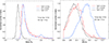 |
Fig. 12. Mass and [Fe/H] distribution (left and right panels, respectively) of the GALAH DR3 giants selected with the same criteria on parameters as in Zhang et al. (2021). All the histograms are scaled to have the same height for the purpose of better visibility. |
To conclude, the results we draw based on GALAH DR3 data are fully consistent with those obtained by Zhang et al. (2021) using LAMOST for giants when we use the same selection criteria for young α-enriched stars. However, while Zhang et al. (2021) call for stellar mergers to explain the mass distribution of their “high-α young giant stars,” based on the fact that 1.2 M⊙ is significantly higher than typical masses of thick disk stars (1 M⊙), our study depicts the effects of secular evolution for a population of y-exαFe giants born with a normal IMF and a [Fe/H] distribution similar to that of their [α/Fe]-normal counterparts. This is in agreement with our conclusions about the y-exαFe dwarf stars.
4. Summary and conclusions
In this paper, we focus, for the first time on dwarf and red giant stars with “extreme” high [α/Fe] values (the upper 1%, independently of their [Fe/H], with [Fe/H] between −1.1 and +0.4 dex), which we call exαFe, and on the youngest of them (ages below 3 Gyr), which we refer to as “y-exαFe”. We selected our sample from the GALAH DR3 survey, applying strict criteria on the precision of the stellar parameters, abundances, and age and mass determinations, and we excluded binaries. We identified a large fraction of y-exαFe stars among both the dwarf and giant exαFe populations (∼30% and ∼15%, respectively) and showed that the [Fe/H] distribution of the exαFe, y-exαFe, and [α/Fe]-normal stars overlap. Beyond the isochrone-based age determination method for single stars provided by GALAH DR3 that we successfully compared to the ages we determined with a different Bayesian tool on another set of stellar models, we explored other indicators of ages, namely, Li abundances for the dwarfs and kinematics for both the dwarf and red giant samples. We also investigated the mass distribution of the overall sample.
As for the y-exαFe dwarf stars, both the Li and the kinematics support their young age. First, the youngest (according to the classical age determination method), hottest, and most massive ones exhibit Li abundances slightly higher (by a factor of 2) than the proto-solar value, in agreement with the Li observed in their young α-normal counterparts. This means that the two populations were born with essentially the same initial Li abundances. Additionally, we find that the exαFe and the α-normal dwarfs undergo the same mass-dependent Li depletion with time, which is also observed in open clusters. Second, the kinematic properties of the y-exαFe dwarf stars (lower eccentricities of their orbits and lower VLSR compare to those of old stars of the thick disk) are similar to those of young [α/Fe]-normal stars, providing strong evidence that they belong to the young stellar population of the thin disk. Finally, after accounting for secular evolution effects and for the magnitude limitations of the GALAH survey that induce artificial patterns in the mass distribution of the entire sample, we showed that y-exαFe dwarfs do not have higher average mass compared to exαFe and [α/Fe]-normal stars.
We also considered exαFe and y-exαFec giants from GALAH, selecting them with the same criteria as for the dwarfs. We did not use the Li indicator, since the first dredge-up induces strong surface Li depletion when the stars become giants, blurring out the information on the initial Li abundance the stars were born with. As for the other properties, our analysis leads to the same conclusions as for the y-exαFe dwarfs. Namely, y-exαFe giants are indeed young both in terms of isochrone-based age determination and kinematics indicators. In addition, they have the same [Fe/H] distribution as young [α/Fe]-normal giant stars. Last but not least, we showed that the position of the peaks in the mass distribution of both the y-exαFe and young [α/Fe]-normal giants results from secular evolution. In particular, the peak at ∼1.9–2 M⊙ we obtain with the adopted age limit of 3 Gyr corresponds to stars at or near the clump. When we increase the age cut, this peak naturally moves towards lower stellar masses that have longer lifetimes, and the RGB peak at lower mass becomes dominant as lower mass stars make it to the red giant phase.
We investigated the impact of the different selection criteria and age limits used in literature studies of giant stars with high [α/Fe]. We showed in particular that the mass and [Fe/H] distributions of the “high-α young giant stars” that lead Zhang et al. (2021) to support the merger scenario is due to a combination of stellar secular evolution and of the adopted limits for both [α/Fe] and the ages of their sample. This strengthens our conclusions that y-exαFe dwarf and giant stars did not form through mergers, but rather with a similar IMF than [α/Fe]-normal stars.
The origins of the y-exαFe stars, which compose ∼0.3% of the large sample of dwarf and red giant stars of the local Galactic population that we selected with strict quality criteria from GALAH DR3, is still unclear. Further studies are needed to check whether their high [α/Fe] ratio reflects massive star ejecta in recent enhanced star formation episodes in the Galactic thin disk, resulting, for instance, from interactions with the Sagittarius dwarf galaxy.
Acknowledgments
This work was supported by the Swiss National Science Foundation (Project 200020-192039 PI C.C.). We extensively used NASA’s Astrophysics Data System Bibliographic Services and TOPCAT (Taylor 2005). We are grateful to A. De Cia, N. Lagarde, V. Hill, and E. Fernández Alvar for enlightening discussions. We are thankful to the anonymous referee for the important comments.
References
- Adibekyan, V. Z., Santos, N. C., Sousa, S. G., & Israelian, G. 2011, A&A, 535, L11 [NASA ADS] [CrossRef] [EDP Sciences] [Google Scholar]
- Almeida-Fernandes, F., & Rocha-Pinto, H. J. 2018, MNRAS, 476, 184 [Google Scholar]
- Amarsi, A. M., & Asplund, M. 2017, MNRAS, 464, 264 [Google Scholar]
- Anders, F., Chiappini, C., Rodrigues, T. S., et al. 2017, A&A, 597, A30 [NASA ADS] [CrossRef] [EDP Sciences] [Google Scholar]
- Andrae, R., Fouesneau, M., Creevey, O., et al. 2018, A&A, 616, A8 [NASA ADS] [CrossRef] [EDP Sciences] [Google Scholar]
- Aumer, M., Binney, J., & Schönrich, R. 2016, MNRAS, 462, 1697 [NASA ADS] [CrossRef] [Google Scholar]
- Baglin, A., Auvergne, M., Barge, P., et al. 2006, in The CoRoT Mission Pre-Launch Status– Stellar Seismology and Planet Finding, eds. M. Fridlund, A. Baglin, J. Lochard, & L. Conroy, ESA Special Publ., 1306, 33 [Google Scholar]
- Bailer-Jones, C. A. L., Rybizki, J., Fouesneau, M., Demleitner, M., & Andrae, R. 2021, AJ, 161, 147 [Google Scholar]
- Bland-Hawthorn, J., & Gerhard, O. 2016, ARA&A, 54, 529 [Google Scholar]
- Bovy, J. 2015, ApJS, 216, 29 [NASA ADS] [CrossRef] [Google Scholar]
- Buder, S., Sharma, S., Kos, J., et al. 2021, MNRAS, 506, 150 [NASA ADS] [CrossRef] [Google Scholar]
- Castro, M., Duarte, T., Pace, G., & do Nascimento, J. D., 2016, A&A, 590, A94 [NASA ADS] [CrossRef] [EDP Sciences] [Google Scholar]
- Charbonnel, C., Lagarde, N., Jasniewicz, G., et al. 2020, A&A, 633, A34 [NASA ADS] [CrossRef] [EDP Sciences] [Google Scholar]
- Charbonnel, C., Borisov, S., de Laverny, P., & Prantzos, N. 2021, A&A, 649, L10 [NASA ADS] [CrossRef] [EDP Sciences] [Google Scholar]
- Chiappini, C., Anders, F., Rodrigues, T. S., et al. 2015, A&A, 576, L12 [NASA ADS] [CrossRef] [EDP Sciences] [Google Scholar]
- Chiba, M., & Beers, T. C. 2000, AJ, 119, 2843 [NASA ADS] [CrossRef] [Google Scholar]
- Deliyannis, C. P., Pinsonneault, M. H., & Charbonnel, C. 2000, in The Light Elements and their Evolution, eds. L. da Silva, R. de Medeiros, & M. Spite, 198, 61 [Google Scholar]
- Dumont, T., Charbonnel, C., Palacios, A., & Borisov, S. 2021, A&A, 654, A46 [NASA ADS] [CrossRef] [EDP Sciences] [Google Scholar]
- Gaia Collaboration (Recio-Blanco, A., et al.) 2022, A&A, in press, https://doi.org/10.1051/0004-6361/202243511 [Google Scholar]
- Gilmore, G., Randich, S., Asplund, M., et al. 2012, The Messenger, 147, 25 [NASA ADS] [Google Scholar]
- Gilmore, G., & Reid, N. 1983, MNRAS, 202, 1025 [Google Scholar]
- Helmi, A. 2020, ARA&A, 58, 205 [Google Scholar]
- Jeffries, R. D., Jackson, R. J., Sun, Q., & Deliyannis, C. P. 2021, MNRAS, 500, 1158 [Google Scholar]
- Larson, R. B., Tinsley, B. M., & Caldwell, C. N. 1980, ApJ, 237, 692 [Google Scholar]
- Lebreton, Y., & Reese, D. R. 2020, A&A, 642, A88 [NASA ADS] [CrossRef] [EDP Sciences] [Google Scholar]
- Loebman, S. R., Roškar, R., Debattista, V. P., et al. 2011, ApJ, 737, 8 [Google Scholar]
- Luo, A. L., Zhao, Y.-H., Zhao, G., et al. 2015, Res. Astron. Astrophys., 15, 1095 [Google Scholar]
- Mackereth, J. T., Bovy, J., Leung, H. W., et al. 2019, MNRAS, 489, 176 [Google Scholar]
- Magazzu, A., Rebolo, R., & Pavlenko, I. V. 1992, ApJ, 392, 159 [Google Scholar]
- Majewski, S. R., Schiavon, R. P., Frinchaboy, P. M., et al. 2017, AJ, 154, 94 [NASA ADS] [CrossRef] [Google Scholar]
- Marigo, P., Girardi, L., Bressan, A., et al. 2017, ApJ, 835, 77 [Google Scholar]
- Martell, S. L., Simpson, J. D., Balasubramaniam, A. G., et al. 2021, MNRAS, 505, 5340 [NASA ADS] [Google Scholar]
- Martig, M., Rix, H.-W., Silva Aguirre, V., et al. 2015, MNRAS, 451, 2230 [NASA ADS] [CrossRef] [Google Scholar]
- Miglio, A., Chiappini, C., Mackereth, T., et al. 2021, A&A, 645, A85 [EDP Sciences] [Google Scholar]
- Mishenina, T. V., Soubiran, C., Kovtyukh, V. V., & Korotin, S. A. 2004, A&A, 418, 551 [NASA ADS] [CrossRef] [EDP Sciences] [Google Scholar]
- Mor, R., Robin, A. C., Figueras, F., Roca-Fàbrega, S., & Luri, X. 2019, A&A, 624, L1 [NASA ADS] [CrossRef] [EDP Sciences] [Google Scholar]
- Osorio, Y., Barklem, P. S., Lind, K., et al. 2015, A&A, 579, A53 [NASA ADS] [CrossRef] [EDP Sciences] [Google Scholar]
- Osorio, Y., Lind, K., Barklem, P. S., Allende Prieto, C., & Zatsarinny, O. 2019, A&A, 623, A103 [NASA ADS] [CrossRef] [EDP Sciences] [Google Scholar]
- Pietrinferni, A., Cassisi, S., Salaris, M., & Castelli, F. 2004, ApJ, 612, 168 [Google Scholar]
- Pietrinferni, A., Cassisi, S., Salaris, M., & Castelli, F. 2006, ApJ, 642, 797 [Google Scholar]
- Pitrou, C., Coc, A., Uzan, J.-P., & Vangioni, E. 2018, Phys. Rep., 754, 1 [Google Scholar]
- Prantzos, N. 2012, A&A, 542, A67 [NASA ADS] [CrossRef] [EDP Sciences] [Google Scholar]
- Prochaska, J. X., Naumov, S. O., Carney, B. W., McWilliam, A., & Wolfe, A. M. 2000, AJ, 120, 2513 [Google Scholar]
- Prša, A., Harmanec, P., Torres, G., et al. 2016, AJ, 152, 41 [Google Scholar]
- Reddy, B. E., Lambert, D. L., & Allende Prieto, C. 2006, MNRAS, 367, 1329 [Google Scholar]
- Ruiz-Lara, T., Gallart, C., Bernard, E. J., & Cassisi, S. 2020, Nat. Astron., 4, 965 [NASA ADS] [CrossRef] [Google Scholar]
- Salaris, M., & Cassisi, S. 2005, Evolution of Stars and Stellar Populations (Wiley-VCH) [Google Scholar]
- Schönrich, R., & Binney, J. 2009, MNRAS, 396, 203 [Google Scholar]
- Sestito, P., & Randich, S. 2005, A&A, 442, 615 [NASA ADS] [CrossRef] [EDP Sciences] [Google Scholar]
- Sharma, S., Stello, D., Buder, S., et al. 2018, MNRAS, 473, 2004 [NASA ADS] [CrossRef] [Google Scholar]
- Silva Aguirre, V., Bojsen-Hansen, M., Slumstrup, D., et al. 2018, MNRAS, 475, 5487 [NASA ADS] [Google Scholar]
- Steinmetz, M., Zwitter, T., Siebert, A., et al. 2006, AJ, 132, 1645 [Google Scholar]
- Steinmetz, M., Guiglion, G., McMillan, P. J., et al. 2020, AJ, 160, 83 [NASA ADS] [CrossRef] [Google Scholar]
- Taylor, M. B. 2005, in Astronomical Data Analysis Software and Systems XIV, eds. P. Shopbell, M. Britton, & R. Ebert, ASP COnf. Ser., 347, 29 [Google Scholar]
- Wang, E. X., Nordlander, T., Asplund, M., et al. 2021, MNRAS, 500, 2159 [Google Scholar]
- Woosley, S. E., Hartmann, D. H., Hoffman, R. D., & Haxton, W. C. 1990, ApJ, 356, 272 [NASA ADS] [CrossRef] [Google Scholar]
- Wu, Y., Xiang, M., Bi, S., et al. 2018, MNRAS, 475, 3633 [NASA ADS] [CrossRef] [Google Scholar]
- Wu, Y., Xiang, M., Zhao, G., et al. 2019, MNRAS, 484, 5315 [NASA ADS] [CrossRef] [Google Scholar]
- Xiang, M., Ting, Y.-S., Rix, H.-W., et al. 2019, ApJS, 245, 34 [Google Scholar]
- Zappala, R. R. 1972, ApJ, 172, 57 [NASA ADS] [CrossRef] [Google Scholar]
- Zhang, M., Xiang, M., Zhang, H.-W., et al. 2021, ApJ, 922, 145 [NASA ADS] [CrossRef] [Google Scholar]
- Zhao, G., Zhao, Y.-H., Chu, Y.-Q., Jing, Y.-P., & Deng, L.-C. 2012, Res. Astron. Astrophys., 12, 723 [NASA ADS] [CrossRef] [Google Scholar]
All Tables
Selection criteria applied to build the different sub-samples of dwarfs we consider in this work.
Selection criteria applied to build the different sub-samples of giants from the GALAH catalog.
All Figures
|
Fig. 1. Kiel diagram for the dwarf and giant stars selected from GALAH DR3. Upper panel: number density plot showing the positions of α-normal stars of the main samples of dwarfs and giants. Squares show the positions of extreme [α/Fe]-rich (exαFe, see Sect. 2.2.1) dwarf stars: y-exαFe (age ≤ 3 Gyr) and older exαFe are shown by blue and red squares, respectively. We keep the same notations, but in circles, for giants. Bottom panel: same details, but for stars in the additional sample (open symbols). |
| In the text | |
|
Fig. 2. Properties of the dwarf stars of the main and additional samples (left and right columns, respectively; see details in Table 1) in the Tinsley–Wallerstein diagram. The solid curve separates the top 1% of stars in each of the 10 metallicity bins from the remaining 99% (exαFe and [α/Fe]-normal stars, respectively), whereas the dashed curve is the median (50% of stars above and below it). From top to bottom: ages, masses, and Li abundances are color-coded, with the color of the background indicating the mean value of the property in bins of size 0.0125 dex in [Fe/H] and 0.0094 dex in [α/Fe]. Individual stars with age ≤3 Gyr and A(Li) ≥ 2.65 dex are also indicated by big and small points for stars above and below the top 1% curve, respectively. |
| In the text | |
|
Fig. 3. Age (top) and [Fe/H] (bottom) distributions of the exαFe (thick black, scale on the left) and [α/Fe]-normal (thin grey, scale on the right) dwarf stars from the main (solid) and additional (dashed) samples. |
| In the text | |
|
Fig. 4. Mass distribution of y-exαFe (top), all exαFe (middle) and [α/Fe]-normal (bottom) stars. Nearby stars (distance D < 200 pc) are on the left panels and all stars up to 2500 pc on the right panels, for the main (solid) and additional (dotted) samples, respectively. |
| In the text | |
|
Fig. 5. Age color-coded A(Li) values as a function of Teff for exαfe and [α/Fe]-normal stars (upper and lower panels, respectively). Left and right columns are for the main and additional samples, respectively. |
| In the text | |
|
Fig. 6. Distribution of eccentricities and velocities with respect to the local standard of rest VLSR (upper and bottom panels, respectively) for y-exαFe and young [α/Fe]-normal dwarfs stars (blue and grey histograms, respectively). The green histogram shows the distribution of old (age ≥ 8 Gyr) stars with [α/Fe] ≥ dex. The magenta histogram shows the distribution of 40 y-exαFe stars with A(Li) > A(Li)SBBN = 2.65. All the histograms are scaled to have the same height and we show the distributions for the main sample only for the purpose of better visibility. |
| In the text | |
|
Fig. 7. Number density plots showing [α/Fe] and [Fe/H] (upper and bottom panels respectively) as a function of age for the main dwarf sample. Color-coded circles show the positions of the y-exαFe stars with A(Li) > 2.65 of the main and additional samples (filled and open circles, respectively) |
| In the text | |
|
Fig. 8. Properties of the giants of the main and additional samples (left and right columns, respectively) in the Tinsley–Wallerstein diagram. Small squares represent bins with more than five stars. Blue points show the positions of young (< 3 Gyr) stars. |
| In the text | |
|
Fig. 9. Age (top) and [Fe/H] (bottom) distributions of the exαFe (thick black, scale on the left) and [α/Fe]-normal (thin grey, scale on the right) giant stars from the main (solid) and additional (dashed) samples. |
| In the text | |
|
Fig. 10. Mass distribution of the giant stars assuming different age limits (3, 4, and 6 Gyr from bottom to top). Red histograms correspond to y-exαFe (i.e., younger than the age cut) giants of the main and additional samples (full and dotted respectively). The blue and black histograms correspond respectively to the young [α/Fe]-normal giants and to exαFe giants older than the cut (for these two cases we show only the distributions of the main sample stars). All the histograms are scaled to have the same height for the purpose of visibility, and the numbers on the left give the number of stars in each color-coded class of giants. |
| In the text | |
|
Fig. 11. Distribution of eccentricities (upper panel) and VLSR of the giants (same colors as in Fig. 10). |
| In the text | |
|
Fig. 12. Mass and [Fe/H] distribution (left and right panels, respectively) of the GALAH DR3 giants selected with the same criteria on parameters as in Zhang et al. (2021). All the histograms are scaled to have the same height for the purpose of better visibility. |
| In the text | |
Current usage metrics show cumulative count of Article Views (full-text article views including HTML views, PDF and ePub downloads, according to the available data) and Abstracts Views on Vision4Press platform.
Data correspond to usage on the plateform after 2015. The current usage metrics is available 48-96 hours after online publication and is updated daily on week days.
Initial download of the metrics may take a while.