| Issue |
A&A
Volume 668, December 2022
|
|
|---|---|---|
| Article Number | A38 | |
| Number of page(s) | 22 | |
| Section | Cosmology (including clusters of galaxies) | |
| DOI | https://doi.org/10.1051/0004-6361/202244263 | |
| Published online | 30 November 2022 | |
Fossil group origins
XII. The large-scale environment around fossil systems
1
Dipartimento di Fisica e Astronomia “G. Galilei”, Università di Padova, Vicolo dell’Osservatorio 3, 35122 Padova, Italy
e-mail: This email address is being protected from spambots. You need JavaScript enabled to view it.
2
INAF – Osservatorio Astronomico di Padova, Vicolo dell’Osservatorio 2, 35122 Padova, Italy
3
Instituto de Astrofísica de Canarias, Calle Vía Láctea s/n, 38205 La Laguna, Tenerife, Spain
4
Departamento de Astrofísica, Universidad de La Laguna, Avenida Astrofísico Francisco Sánchez s/n, 38206 La Laguna, Spain
5
INAF – Osservatorio Astronomico di Trieste, Via Tiepolo 11, 34143 Trieste, Italy
6
Dipartimento di Fisica, Università degli Studi di Trieste, Via Tiepolo 11, 34143 Trieste, Italy
Received:
14
June
2022
Accepted:
29
July
2022
Abstract
Aims. We analyse the large-scale structure out to 100 Mpc around a sample of 16 confirmed fossil systems using spectroscopic information from the Sloan Digital Sky Survey Data Release 16.
Methods. We computed the distance between our fossil groups (FGs) and the centres of filaments and nodes from the literature. We also studied the density of bright galaxies, since this parameter is thought to be a good mass tracers, as well as the projected over-densities of galaxies. Finally, we applied a friends-of-friends (FoF) algorithm to detect virialised structures around our FGs and obtain an estimate of the mass available in their surroundings.
Results. We find that FGs are mainly located close to filaments, with a mean distance of 3.7 ± 1.1 R200 and a minimum distance of 0.05 R200. On the other hand, none of our FGs were found close to intersections, with a mean and minimum distance of 19.3 ± 3.6 and 6.1 R200, respectively. There is a correlation that indicates FGs at higher redshifts are found in denser regions, when we use bright galaxies as tracers of the mass. At the same time, FGs with the largest magnitude gaps (Δm12 > 2.5) are found in less dense environments and tend to host (on average) smaller central galaxies.
Conclusions. Our results suggest that FGs formed in a peculiar position within the cosmic web, close to filaments and far from nodes, whereby their interaction with the cosmic web itself may be limited. We deduce that FGs with brightest central galaxies (BCGs) that are relatively faint, high values of Δm12, and low redshifts could, in fact, be systems that are at the very last stage of their evolution. Moreover, we confirm theoretical predictions that systems with the largest magnitude gap are not massive.
Key words: galaxies: clusters: general / galaxies: groups: general
© S. Zarattini et al. 2022
 Open Access article, published by EDP Sciences, under the terms of the Creative Commons Attribution License (https://creativecommons.org/licenses/by/4.0), which permits unrestricted use, distribution, and reproduction in any medium, provided the original work is properly cited.
This article is published in open access under the Subscribe-to-Open model. This email address is being protected from spambots. You need JavaScript enabled to view it. to support open access publication.
1. Introduction
Fossil groups (FGs) were proposed by Ponman et al. (1994) upon their discovery of an apparently isolated giant elliptical galaxy that was surrounded by an X-ray halo typical of a group of galaxies. These authors’ interpretation of these observations was that this system was the final stage of evolution of a galaxy group, in which all the other M* galaxies (where M* is the characteristic luminosity of the luminosity function) were merged within the brightest central galaxy (BCG). To explain this scenario, FGs were assumed to be older than regular groups and to remain isolated from the cosmic web. In this picture, FGs can be considered fossil relics of the primordial Universe.
It is only in the last decade that the number of known FGs has grown large enough so as to have a basis for systematic studies of these objects. While far from being exhaustive, four over-luminous red galaxies were given in Vikhlinin et al. (1999), five FGs were presented in Jones et al. (2003), 34 FG candidates were proposed in Santos et al. (2007), with 15 confirmed in Zarattini et al. (2014), 12 new FGs were presented in Miller et al. (2012). In addition, 18 FG candidates were presented in Adami et al. (2018), while in Adami et al. (2020) a novel probabilistic approach was used to favour statistical studies of FGs. Recently, a list of 36 confirmed FGs (taken from the literature) was presented in a review by in Aguerri & Zarattini (2021), across the redshift range of 0 ≤ z ≤ 0.5.
The hierarchical model of structure formation in the Universe is a remarkably successful theory. It predicts that small structures form earlier and that they subsequently collapse into larger structures. This model is proven to be successful at large scales, however, on galactic scales, it incurs the so-called ‘small-scale crisis’, namely: the number of predicted low-mass sub-halos in simulations around Milky-way like galaxies is greater than we see from observations. On the other hand, D’Onghia & Lake (2004) found that the small-scale crisis could be affecting the larger halos of FGs and that, in this case, the missing satellites may be as massive as the Milky Way itself. However, Zibetti et al. (2009) and Lieder et al. (2013) found no signs of missing satellites in FGs.
The Fossil Group Origins project (FOGO, Aguerri et al. 2011) is devoted to the study of one of the largest sample of FGs available in the literature. The previous eleven publications from the FOGO team have shed light onto various aspects of FGs. In particular, the formation of their BCGs were studied in Méndez-Abreu et al. (2012), whereas their stellar populations were analysed in Corsini et al. (2018). In these works, the authors showed that BCGs in FGs are amongst the most massive galaxies in the Universe and that their stellar age is compatible with central galaxies in non-fossil systems. At the same time, BCGs are found to be more segregated in the velocity space when compared to non-FGs (Zarattini et al. 2019). The scaling relations between the optical and X-ray bands (Girardi et al. 2014; Kundert et al. 2015) showed that FGs were not X-ray over-luminous systems and that particular attention must be paid to the homogeneity of the data in these kind of studies. In addition, the luminosity functions (LFs) of FGs were compared with those of non-FGs (Zarattini et al. 2015; Aguerri et al. 2018), finding that there is a dependence of the faint-end slope on the magnitude gap. Moreover, FGs were found to host a similar fraction of substructures as non-FGs (Zarattini et al. 2016). Finally, in Zarattini et al. (2021), we showed that one of the main differences between fossil and non-fossil systems can be found in the different orbital shape of their galaxies. In fact, we found that galaxies falling into FGs are more likely to be seen on radial orbits than in non-FGs, which is in agreement with theoretical predictions (Sommer-Larsen et al. 2005).
Only a few works have been devoted to the study of the large-scale environment around FGs. In particular, Adami et al. (2012) compared the environment of two FGs with one non-FG using photometric data. They found FGs to be more isolated than the control cluster, but the statistic was quite low and prevented them from reaching general conclusion. In a similar way, Adami et al. (2018) used the spectroscopic data of RXJ1119.7+2126 (one of the two FGs of their previous paper) and were able to confirm that this system is located in a poor environment.
The aim of this work is thus to analyse the large-scale structure around a large sample of spectroscopically confirmed FGs in order to understand if they are found in any peculiar position of the cosmic web. The cosmology used in this paper, as in the rest of the FOGO publications is H0 = 70 km s−1, Ωλ = 0.7, and ΩM = 0.3.
2. Sample selection
We selected our sample from the review of Aguerri & Zarattini (2021), where a list of spectroscopically-confirmed FGs in presented in their Table 1. In particular, we chose all the systems whose centres have been found within the footprint of the Sloan Digital Sky Survey Data Release 16 (SDSS DR16), and with an upper redshift limit of z = 0.20. The SDSS spectroscopy is mainly limited at mr = 17.77, which is equivalent to Mr ∼ −22 at z = 0.2. The central galaxies of this sample have magnitudes ranging between Mr = −21.3 and Mr = −24.1, so the faintest of the sample would not be mapped at z = 0.2. We thus decided to limit the sample to z = 0.15, corresponding to a magnitude limit of Mr ∼ −21.5. The systems selected according to these criteria amount to 18. We note that we also included SDSS J1045+0420, at a redshift of z = 0.154.
We thus looked at the spectroscopic completeness of the various clusters. In fact, it is possible that some cluster is part of the SDSS footprint, but for some reason its spectroscopy is below the standard. We computed the fraction of galaxies with spectroscopy by considering the number of galaxies with spectroscopy and the number of targets (e.g., galaxies with mr ≤ 17.77). In Fig. 1, we can see that only two clusters have a completeness lower than 65%: these are UGC 842 and 1RXS J235814.4+150524. The former is found in a region of SDSS with very uneven spectroscopic coverage, while the latter would also be discarded using the redshift criterium, so we did not check its spectroscopic coverage in detail. We ended up with 17 FGs after applying this cut.
 |
Fig. 1. Spectroscopic completeness for our starting sample. The two systems with completeness smaller than 65% were not included in our final sample. |
In Sect. 2.2, we explain why we prefer to exclude FGS28 from our sample, given its dubious nature. Ultimately, our final sample is thus composed of 16 FGs, whose properties are presented in Table 1. We note that the coordinates reported in the table are those of BCGs, namely, galaxies with homogeneous centres. In fact, for some systems (e.g., FOGOs) the centre reported in the literature is that of the BCG; for some others, the centre reported in the literature was obtained from X-ray data. There is a known discrepancy between these two centres, estimated in 13 kpc in Sanderson et al. (2009) using a sample of 65 X-ray-selected clusters and in less than 5% of R200 from Lin et al. (2004). Moreover, Aguerri et al. (2007) compared the distance between the X-ray peak and the galaxy surface density, finding a mean difference of 150 kpc. We do not expect this difference to impact in the results of our work, since all our tests involve megaparsec scales. Moreover, magnitude gaps (within 0.5 R200) and X-ray luminosities were also taken directly from Aguerri & Zarattini (2021) and references therein. However, in Sect. 2.1, we explain how we converted the LX values to bolometric LX luminosities and to the same cosmology used in this paper. On the other hand, only a few mass values were available in Aguerri & Zarattini (2021) and references therein, so we decided to estimate them by using their bolometric X-ray luminosities, thus homogenising the computation.
Global properties of the sample.
The SDSS catalogues were obtained with an SQL query to the CasJobs webpage1. For each system, we looked for all galaxies with available spectroscopy within a radius of 100 Mpc from the centre of the system reported in Table 1. It is worth noting that for some clusters, it was not possible to obtain data for the entire 100-Mpc-radius area. In Appendix A, we present the entire field of view (FoV) available for each cluster. For eight clusters, the full area is covered (11 if we consider a circle of 50 Mpc radius). For the remaining clusters, the coverage is not full, but we can still use them for the majority of our scope.
2.1. LX luminosities
We were able to obtain the X-ray luminosity for all the systems in the sample. All the LX values were taken from the literature and were computed according to different bands, cosmologies, and methods. We then converted all the LX to the same band and cosmology. In particular, we chose to convert to bolometric luminosity and to the cosmology of this paper when needed.
Bolometric luminosities were obtained by multiplying the luminosity in the different bands by a temperature-dependent correction factor. In particular, we found luminosities in the 0.1 − 2.4 keV (two FGs) and 0.5 − 2.0 keV bands (seven FGs); the remaining seven FGs already had their bolometric data established. This factor was computed using the Raymond-Smith code with ICM of 0.3 Z⊙, according to the PIMMS2 webpage.
The code requires the input of the X-ray temperature TX. The values of TX are available in the literature for seven out of nine clusters. For the remaining two clusters, we followed a recursive procedure based on the TX − LX relation (see Girardi et al. 2014). The values of the (bolometric) X-ray luminosities are listed in Table 1.
2.2. FGS28
The fossil group FGS28 is found at z = 0.032. There are four other clusters nearby: NGC 6107 (z = 0.0315), A2192 (z = 0.0317), A2197 (z = 0.0301), and A2199 (z = 0.0299). The largest velocity difference between all of them is ∼600 km s−1. The pair A2197 and A2199 is considered as a supercluster in the literature (Rines et al. 2002) and it is known to be connected via a large filament to the Hercules supercluster (Ciardullo et al. 1983). The A2197 mass profile (the closest to the position of FGS28) is better fitted by dividing the cluster in two clumps named ‘east’ and ‘west’ in Rines et al. (2002).
Moreover, in Zarattini et al. (2014) we found that FGS28 was peculiar, since it has only one member within R200 and there were another four members outside this area. Our interpretation is that this is not a real group of galaxies – and that, rather, it is a giant galaxy that is part of the A2197/A2199 supercluster. For these reasons, we opted to remove FGS28 from our sample of FGs.
3. Fossil systems position in the large-scale structure
In this section, we discuss how we defined the large-scale structure around our FGs. In particular, in Sect. 3.1, we introduce the catalogue of filaments presented in Chen et al. (2016) and we compute the distance of the FGs in our sample from the centre of filaments and intersections. Then, in Sect. 3.2, we explain in detail how we applied a friends-of-friends (FoF) algorithm to our FGs and the results of that application.
3.1. Catalogue of filaments
The first method we used to study the large-scale structure of our FG sample analysing their position with respect to the catalogue of filaments presented in Chen et al. (2016). In this catalogue, the filaments were found using SDSS data by applying the Subspace Constrain Mean Shift (SCMS) algorithm based on galaxy density ridges. In particular, SCMS performs three steps to detect filaments (density estimation, thresholding, and gradient ascent; see Chen et al. 2015, and references therein). To build the catalogue, the authors used spectroscopically-confirmed galaxies in the redshift range of 0.05 < z < 0.7, divided into 130 redshift bins. As a result, the filament catalogue only covers this redshift range and it is limited in RA and Dec (109 ≲ RA ≲ 267 and −4 ≲ Dec ≲ 70).
This approach is similar to that used in Adami et al. (2020), where data from the Canada France Hawaii Telescope Legacy Survey (CFHTLS) was used to detect FG candidates based on photometric redshifts and then a catalog of filaments and nodes obtained from the same CFHTLS was used to study the position of their FG candidates with respect to the large-scale structure of the Universe.
At this point, we have the ability to measure the distance of our FGs from the centre of the filaments for most of our systems. In particular, we computed the distance in RA and Dec between our FGs and the closest filaments in the redshift space. The filament catalogue gives the minimum redshift of the filament (zlow) and all the galaxies in the filament satisfy zlow ≤ z ≤ zlow + 0.005. This means that in the velocity space, each filament is ∼1500 km s−1 wide.
We then measured the distance in RA and Dec from the centre of each FG and the centre of the closest filament. We use this definition because in the catalogue from Chen et al. (2016) the position of the centre of the filament (in both Ra and Dec and in the redshift space) is given. We only use filaments that are found within z ± 0.005 from the target – again equivalent to ±1500 km s−1, as above. We repeat the same computation for determining the distance of each FG to the closest intersection, which is also provided in the Chen et al. (2015) catalogue. In Fig. 2, we show the relation between the magnitude gap (Δm12), the X-ray luminosity (LX), and the absolute magnitude of the central galaxy (Mr, BCG) and the distance from the center of the filaments (left panels) or intersections (right panels), as defined in Chen et al. (2016). It is interesting to note that the majority of the FGs in our sample are found nearby filaments, with a mean distance of 3.7 R200 and a minumim distance of 0.05 R200. On the other hand, the distance between our FGs and the intersections is larger, with a mean of 19.3 R200 and a minimum distance of 6.1 R200, as shown in Table 2. In the same table, the distance between each FG and the center of the closest filament is reported, but in Appendix A, we show the entire large-scale structure around each FG for an easier visual inspection. It is worth noting that for AWM4, we were not able to compute the distance from filaments and intersections, since this FG exhibits z = 0.0317, a value below the redshift limit of the Chen et al. (2016) catalogue (z = 0.05).
 |
Fig. 2. Correlations between Δm12 (top panel), Mr, BCG (middle panel), and LX (lower panel) and the distance to the filament (left column) in units of R200. Same parameters correlated with the distance to the intersections (right column). The dashed horizontal line in the left panel represents 5 R200, which is the distance that we used to separate FGs that are close to filaments (Dfila < 5 R200, blue diamonds) from those that are not (red stars). |
Distance to filaments and intersections for the FGs in our sample.
We were thus able to split our FGs into two categories: systems that are found in a region close to a filament (Dfila ≤ 5 R200) and systems that are more isolated. The separation is shown in Fig. 2 with an horizontal line and in the entire paper, FGs close to filaments are shown in blue, whereas red represents FGs that are far from filaments. With regard to AWM4, for which the distance to filaments and node was not computed, is shown in black. However, no correlation was found between Δm12, LX, and Mr, BCG and the distance to filaments or intersections.
3.2. Friend-of-friends algorithm
We also ran a friends-of-friends algorithm on our data. The algorithm was presented in Calvi et al. (2011) and was applied to all the galaxies within ±3000 km s−1 from the velocity of the parent cluster.
Two parameters were used to define the ‘friends’, namely: a linking length and a linking velocity. For the former, as a first attempt, we ran the FoF algorithm by using a single linking length of 0.5 Mpc to select the core of the clusters and reduce the number of contaminant galaxies. However, the results worsened with z: at low redshift (z < 0.1), the FoF output follows the visible large-scale structure of each system, but at z > 0.1, where the data are less sampled, almost nothing was found by the algorithm. Thus, we used a variable linking length depending on redshift: in particular, we used 0.5 Mpc for z < 0.05, 1.0 Mpc for 0.05 ≤ z < 0.1, and 1.5 Mpc for z ≥ 0.1. This choice was made in order to reflect the smaller number of galaxies found when increasing the redshift. In fact, SDSS spectroscopy is limited in apparent magnitude (down to r ≤ 17.77), which means that increasing redshift will result in a decrease in the number of targets. As a result, the mean distance between galaxies with spectroscopy is expected to grow larger. On the other hand, the velocity link was chosen to be constant and fixed at ±1500 km s−1. This choice is motivated by the fact that the majority of clusters have velocity dispersions between 300 and 1000 km s−1 (Munari et al. 2013). We thus assume that ±1500 km s−1 is enough to include the vast majority of galaxy members, without including too many contaminant galaxies.
In Appendix A, the results of the FoF algorithm are presented in red, indicating that a good agreement between red points and the filamentary structures presented in Sect. 3.1 can be found. However, an exact measurement of the precision of the match is beyond the scope of this paper and, in the rest of this work, the filament catalogue is used as the operational definition of the large-scale structure.
Once the FoF results have been obtained, the code looks for virialised structures (e.g., clusters) by computing the R200 radius and the velocity dispersion of the group or cluster, removing the outliers and repeating the process until the number of members converges. For our analysis, we limited the detection of a structure to agglomerations of galaxies that have at least three members and a minimum velocity dispersion of 200 km s−1, namely, the mean velocity dispersion of galaxy groups found using the same FoF algorithm in Calvi et al. (2011). The goal of this cut is to remove smaller structures such as galaxy pairs or smaller groups (Calvi et al. 2011, who found that only 11% of their groups have σV < 100 km s−1) that we believe are not useful for our work. After convergence, we estimate the mass of each structure (details given in Sect. 5.3). The main goal of this procedure is to estimate the mass of groups and clusters around our sample of FGs and to check if there is a relation between the available mass and some of the FG properties. However, sometimes the FG is detected as well and in such cases, we are able to estimate the mass in this alternative way. The FoF-computed mass of each FG is presented in Appendix A.
4. General properties
In Fig. 3, we show the correlations between some of the main parameters available for our sample. In particular, we focus our attention on the magnitude gap (Δm12), the X-ray luminosity (LX), the absolute magnitude of the central galaxy (Mr, BCG), and the virial radius (R200). Some correlations are visible, such those between R200, LX, and the absolute magnitude of the BCG. The R200 − LX correlation is expected, since the former quantity was computed from the latter. Also the R200 − Mr, BCG and the LX − Mr, BCG correlations are expected for all clusters, since massive clusters generally host massive BCGs (Lin et al. 2004; Brough et al. 2008). For our goal, it is more interesting to analyse correlations involving the magnitude gap: it can be seen that there is no clear correlation when using this parameter. The only interesting result is that systems with the largest magnitude gap (Δm12 ≥ 2.5) are small, with LX < 1043 and R200 < 0.7.
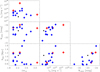 |
Fig. 3. Comparison between the main general properties of the clusters in our sample. Colour code is the same as in Fig. 2, but here we also show AWM4 as a black dot, since this FG is found at a redshift where the Chen et al. (2016) catalogue is not available and thus it cannot be classified based on its distance to a filament. |
Finally, no specific correlation is found for FGs that are close and far from filaments, although systems with Δm12 ≥ 2.5 are mainly close to filaments. However, the one with the largest Δm12 is far from the closest filament and the statistic is generally very poor for these systems.
We then computed the cumulative distribution of Δm12, LX, R200 and Mr, BCG in the two subsamples (e.g., FGs close and far from the centre of filaments). The results, presented in Fig. 4, show that they follow similar relations, with the exception of the absolute magnitude of the BCG. In fact, the three systems that are far from filaments have all BGCs with Mr < −23.5, whereas those close to the centre of filaments are more equally distributed in the range of −24 ≤ Mr ≤ −21.5.
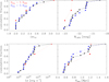 |
Fig. 4. Cumulative distribution of Δm12 (top left panel), absolute magnitude of the BCG (top right panel), X-ray luminosity (bottom left panel), and R200 (bottom right panel). In each panel, the full FG population is described with the solid black line and black circles, FGs close to filaments are represented with blue dashed line and diamonds, and FGs far from filaments are shown with red dashed-dotted line and stars. |
5. Large-scale mass distribution
In this section, we discuss the large-scale environment of FGs with respect to the quantity of mass available in their surroundings and its distribution. Since SDSS spectroscopic data are not homogeneous, the main issue is how to compute precise areas for all the sample, especially for those FGs whose mappings are broadly incomplete. For this reason, in Sect. 5.1, we discuss the Pick theorem and how we use it for our scope. Once the areas are known, we can compute the local projected over-density, described in Sect. 5.2. Finally, in Sect. 5.3, we analyse the quantity of mass available in the FGs’ surroundings by using different indicators: the density and cumulative distribution of bright galaxies as well as the mass found in groups and clusters from the FoF algorithm.
5.1. Pick’s theorem
Pick’s theorem (Pick 1899) states that if a regular polygon has integer coordinates for the vertices, the area can be computed as:
 (1)
(1)
where i is the number of integer points inside the polygon and b is the number of integer points on its boundaries. We used this theorem to compute the area available for each FG in the sample. In particular, we divided our areas into different rectangles and we then applied Pick’s theorem to these now regular polygons.
To estimate the uncertainties, we applied the theorem for those FGs for which the entire 100 Mpc area were available (eight systems). The mean difference between the Pick area and the geometric one is −2.3%, with a maximum of −3.2%. We also compute the difference in the area of 50 Mpc for the 11 systems fully covered out to this radius: in this case, the mean percent error is −3.2%, with a maximum error of −4.2%. The errors are larger in the second case because the number of points used to apply the Pick’s theorem is smaller.
We highlight that the differences in measurements are always negative. This means that the Pick’s theorem is systematically underestimating the geometric areas. Since the errors are connected to the number of available points, we expect to have larger errors for the farthest FGs, since we are using a sample of galaxies that is limited in apparent magnitude.
5.2. Local projected over-densities
At this step, we are able to compute the local over-densities within circular coronas around our FGs. In particular, we used Pick’s area for the coronas and only galaxies within ±1500 km s−1 and mr ≤ 17.77 (the SDSS completeness limit for the main spectroscopic sample). Finally, we corrected for spectroscopic completeness. The over-density is computed as:
 (2)
(2)
where Σ(r) is the density at each specific bin radius and  is the mean density computed by using all galaxies between 20 and 50 Mpc. In particular, we first analysed the over-densities for systems that are closer or farther than 5 R200 from the centre of the closest filament. No difference was found within the errors in this case, as it can be seen in the top panel of Fig. 5. Then, we computed the over-densities by dividing our sample into systems with bright and faint central galaxies, using Mr = −23 as separation. The result is shown in the central panel of Fig. 5 and, in this case, a difference is found in the very central distance bin, at least at the 1-σ level. Finally, in the bottom panel of Fig. 5, we plot the over-densities of our systems divided using X-ray luminosity, which serves as a proxy for the mass of our systems. Again, no difference was found for the over-densities of small or massive FGs.
 |
Fig. 5. Top panel: galaxy over densities for systems with distance to filament larger and smaller than 5 R200 (red open circles and blue filled circles, respectively). Middle panel: same quantities but for systems with bright (Mr < −23) and faint (Mr > −23) central galaxies (green filled diamonds and pink empty diamonds, respectively). Bottom panel: same quantities but for systems with high (LX > 1043) and faint (LX < 1043) X-ray luminosities (azure filled squares and violet open squares, respectively). |
5.3. Available mass in FGs’ surroundings
In order to estimate the mass available in the surrounding of our FGs, we used a set of indicators. First of all, we computed the density of bright galaxies (Mr < −22) per Mpc2 that are found within 50 Mpc from the centre of the FG. The area in degrees was obtained using Pick’s theorem, as explained in Sect. 5.1, to have a proper estimate also for systems that are not fully covered in the 50 Mpc radius. In Fig. 6, we show the correlations between the absolute magnitude of the BCGs, the magnitude gap, the redshift, and the X-ray luminosities versus the density of bright galaxies. The most relevant result is obtained for the Δm12− density correlation: systems with the largest magnitude gap are always found in low-density regions, whereas systems with the smallest gaps are found in all environments. We repeated the computation using galaxies with Mr ≤ −23, finding exactly the same trend, although with fewer statistics, and for this reason, we prefer to show the results with Mr ≤ −22 here.
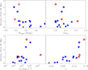 |
Fig. 6. Correlations between the absolute magnitude of the BCG (top left panel), the magnitude gap (top right panel), the X-ray luminosity (bottom left panel), and redshift (bottom right) vs. the density of galaxies brighter than −22 within 50 Mpc. The area is computed using Pick’s theorem, so footprint incompleteness is properly taken into account. Colour coding and symbols are the same as in Fig. 2. Big open circles represent FGs with central galaxies brighter than −22. |
Another useful indicator is the cumulative distribution of bright galaxies, that is shown in Fig. 7. It can be seen that no differences are found within 50 Mpc between FGs close and far from filaments. A Kolmogorov–Smirnov (KS) test confirms this result by giving a KS probability of 0.99, where differences in the two distributions are expected if this value is smaller than 0.05. However, in the first panel of Fig. 7, small differences seem to appear in the central and external regions: in the former, a smaller number of bright galaxies are found in FGs close to filaments, whereas the opposite is found in the latter. We thus compute the cumulative distribution in a smaller area, namely, 20 Mpc, aiming at looking in more details to the differences in the neighborhood of our FGs. Although the difference is visually larger, a KS test confirms that both distributions (FGs close and far from filaments) come from the same parent distribution (KS probability of 0.99 also in this case), so we conclude that no difference is found in the distribution of bright galaxies within 50 Mpc from our FGs and, thus, we did not test the external regions.
 |
Fig. 7. Cumulative distribution of bright galaxies (Mr < −22) in 50 Mpc (left panel) and 20 Mpc (right panel). The colour coding is the same as in Fig. 2. |
The FoF algorithm that we used is able to identify virialised objects and to estimate their velocity dispersion. Thus, we used it to estimate the mass of these virialised systems according to Eq. (1) of Munari et al. (2013). In Fig. 8, we plot the correlation between total mass available within 50 and 100 Mpc and some global quantities of the FG in our sample, namely, the magnitude gap, the absolute magnitude of the BCG, the X-ray luminosity, the virial radius, and the redshift. There are 11 FGs well mapped out to 50 Mpc and 8 fully mapped out to 100 Mpc. No particular trend was found, except the one between the available mass and the X-ray luminosity. In fact, it seems that the most luminous FGs have less mass available, but this result can be driven by a couple of points in the most extreme regions of this relation. We ran a Spearman correlation test (Spearman 1904) that found a significant correlation (ρ ∼ 0.02) between the X-ray luminosity and the available mass within 50 and 100 Mpc. In both cases, there is a negative correlation (the available mass decreases while the X-ray luminosity increases). Other weak correlations were also found, such as one between the virial radius and the mass found in 100 Mpc (ρ ∼ 0.09) and another between the redshift and the mass found in 50 Mpc (ρ ∼ 0.06). The latter trend is apparently the opposite of the one found between redshift and the density of bright galaxies (further discussed in Sect. 6).
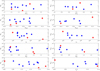 |
Fig. 8. Correlations between the mass found by the FoF algorithm within 50 or 100 Mpc (left and right columns, respectively) and some global quantities of our sample. The colour coding is the same as in Fig. 3. |
6. Discussion
The results presented in this paper can be interpreted in terms of the formation scenario and evolution of FGs. We show that the majority of the FGs in our sample are found close to the centre of filaments, with a mean distance of 3.7 ± 1.1 R200, whereas, none have been found close to intersections (mean distance of 19.3 ± 3.6 R200). This is surprising, since usually galaxy groups and clusters are though to form in the nodes of the cosmic web (e.g., Cautun et al. 2014). These models predicts that the feeding mechanism for galaxy clusters is based on their receiving new objects falling along filaments into the node. The position of FGs, namely, far from the nodes could thus be the responsible for the formation of their wide magnitude gap. In fact, Ponman et al. (1994) first suggested that FGs could have been isolated from the cosmic web, whereby they have more time to merge all their bright galaxies with the BCG without receiving more bright galaxies from their nearest surroundings. Our results seem to favour this scenario, in which objects that are moving within the filaments are not able to leave them to reach the nearby FGs. However, it is difficult to estimate the size of filaments, in particular, its width or thickness. For this reason, we are not able to definitively claim that FGs are found embedded in filaments or just outside them.
It is interesting to note that our results are in good agreement with what was found in Adami et al. (2020), where the authors analysed a sample of FG identified using a probabilistic approach in the CFHTLS, finding that FGs seem to reside closely to cosmic filaments and do not survive in nodes. In particular, 87% of their FGs are within 1 Mpc to a filament, whereas 67% are farther than 1 Mpc from any nodes. We have found a similar trend, but we only have 33% of our FGs within 1 Mpc from a filament. This fraction rises to 73% if we consider systems within 2 Mpc from the centre of the filament. This difference can be due to the different cuts used in Adami et al. (2020) to define filaments and nodes close (in the redshift space) to their target FGs: in fact, since they worked with photometric redshift instead of spectroscopic ones, their filament catalogue uses slices that are thicker than ours, possibly leading to projection effects, namely: more filaments and nodes in the same projected area with respect to Chen et al. (2016), as they noted in their work. A similar conclusion can be reached for the distance from the nodes, with the difference that all our FGs (100%) are farther than 1 Mpc from nodes, whereas in Adami et al. (2020), they found 67%. We need to use a distance of 10 Mpc to recover a similar fraction for our sample (60%). Again, differences in the construction of the catalogues of filaments and nodes or applying a different strategy when analysing the data could lead to these differences that, we note, are quantitative rather than qualitative.
Within this scenario, it is also interesting to note that FGs with the largest magnitude gaps are not massive (all the four systems with Δm12 ≥ 2.5 have LX < 1043 erg s−1). This can be a boost for the merging timescale of bright galaxies within this systems, since the available mass is smaller (with fewer massive galaxies) and the relative velocity between galaxies is smaller too, due to the shallower gravitational potential that groups have with respect to clusters. These two conditions, together with the presence of more radial orbits expected in FGs (as predicted theoretically and observationally confirmed in Sommer-Larsen et al. 2005; Zarattini et al. 2021) are the main ingredients that reduce the timescale of dynamical friction (see Eq. (4.2) in Lacey & Cole 1993).
Dariush et al. (2010) suggested that only FGs with small central galaxies could be real FGs, purported to be systems with an older formation age than regular groups and clusters that have passively evolved without many interactions with the cosmic web. At this point, we can suggest that these old FGs could be those found outside of cosmic filaments, whose peculiar position blocks further accretion.
Our results support a scenario in which FGs stand as a transitional stage in the life of a group or cluster and that the magnitude gap can be reduced when a bright galaxy falls into the FG potential (Aguerri et al. 2018; Kim et al. 2022). However, we found that the largest gaps are found in FG with a low density of bright galaxies around them. In particular, systems with Δm12 ≥ 2.5 have less than one galaxy brighter than Mr = −22 within 50 Mpc, whereas five out of ten systems with Δm12 < 2.5, have more than one bright galaxy within their 50 Mpc radius. This could mean that systems with 2.0 ≤ Δm12 ≤ 2.5 can still be changing their gaps and become non-fossils (because they are closer to Δm12 = 2.0 and they have more bright galaxies nearby), but that FGs with Δm12 > 2.5 are probably less inclined to change the gap to values smaller than Δm12 = 2.0.
A similar suggestion can be obtained for the most isolated FGs, since they presents only very bright BCGs and they are, on average, quite massive. In this case, the boost in the merging timescale could have been given by the higher available mass for the satellite galaxies, whereas their isolation from both filaments and nodes could have avoided the subsequent arrival of new massive satellites. However, the paucity of isolated FGs prevents us from reaching a robust conclusion for this subsample, since only three FGs are isolated in our sample.
We also analysed the galaxy over-density within 100 Mpc. We confirmed that at very large radii (r > 20 Mpc), no differences can be found, with an over-density that oscillates around zero. However, when dividing the sample of FGs into those with bright and faint BCGs, a difference can be found (at 1-σ level) in the most central distance bin: systems with brightest galaxies are found in greater over-densities. This could be connected with a larger number of bright satellites available for merging massive nearby BCGs. On average, FGs with BCGs brighter than −23 have 1.5 ± 1.1 bright galaxies within 50 Mpc, whereas FGs with BCGs fainter than −23 have 0.6 ± 0.4 of these galaxies available. This result is not statistically significant, however, we note that the latter systems have all less than 1 bright galaxy within 50 Mpc, whereas the former systems spread the entire range between 0 and 3.4 bright galaxies within 50 Mpc.
However, other correlations appear when comparing the density of bright galaxies with the global properties of our FGs. First of all, a correlation between LX and the density of bright galaxies is found, where systems with small LX seem to be more isolated. We ran a Spearman test, which showed a positive correlation (coefficient of 0.56) and rejected the null hypothesis (probability of 0.02). Moreover, a correlation between redshift and the density of bright galaxies was found as well (Spearman coefficient and probability of 0.85 and 3 × 10⁻⁵, respectively). The first interpretation could be a sort of selection effect due to observations. However, Verevkin et al. (2011) showed that the redshift distribution in the SDSS-DR7 is peaked at z ∼ 0.08 and then quickly drops at higher redshift. We did not expect this distribution to change in more recent data releases, since the complete main spectroscopic sample (the one that we are using here, limited to mr = 17.77) was released with DR7. Newer SDSS releases indeed include a broader redshift range, but the target selection is different and focussed on high-redshift galaxies (e.g., the BOSS survey, Dawson et al. 2013).
If a selection effect were present, we would also expect the density to be higher for a low-redshift object, however, that is not the case. In fact, we find the opposite correlation. Our interpretation of this result is that FGs at higher redshift are still found in lively environments, where some major merger can still happen. Indeed, this relation can be seen as an indicator of merger probability, higher for systems at higher redshifts, where more bright galaxies (e.g., more mass) are available. Using numerical simulations, Kundert et al. (2017) showed (as seen in the middle-left panel of their Fig. 7) that the number of major mergers in FGs is still growing in the redshift range 0.2 ≲ z ≲ 0.1, whereas it stops growing for z ≲ 0.1; this result may explain what we found in the correlation between redshift and density of bright galaxies.
We also studied the mass available around FGs using the FoF algorithm. In this case, we found an opposite trend with z: the mass available (within 50 Mpc) is higher for systems at low redshift. However, we believe that this result can be more affected by biases. In fact, we used different (and arbitrary) linking length for systems with varying redshifts. This was done for the purpose of obtaining a good visual agreement between the filaments of Chen et al. (2016) and the FoF galaxies. Since the linking length is smaller for systems at low redshift (0.5 Mpc for z < 0.05 versus 1.5 Mpc for z > 0.1), we can expect an excess of linked galaxies in the lowest redshift FGs. Moreover, we have also excluded small groups from the FoF computation, thus again favouring the detection of groups at low redshifts, where the density of data is higher. Finally, the density of bright galaxies is more robust when using a survey limited in apparent magnitude, as the SDSS. In fact, Mr = −22 is equivalent, at z = 0.15, to mr = 17.2, which means that the SDSS spectroscopy (e.g., the galaxies used in this work) is also complete at these redshifts.
In conclusion, we found that the very large-scale environment (distances larger than 10 Mpc) does not play any role in the evolution of FGs. Hints have been found that some difference can be due the environment at distances smaller than 10 Mpc. This can be due to the presence of filaments, whose mean distance is 3.7 R200 (or 3.0 Mpc).
7. Conclusions
We analysed a sample of 16 FGs with z ≤ 0.15, for which the magnitude gap was spectroscopically confirmed to be Δm12 ≥ 2, and with spectroscopic completeness greater than 65% in SDSS-DR16.
The aim of this work is to test the large-scale environment surrounding FGs. For this purpose, we downloaded and analysed all the spectroscopic data available in the SDSS DR16 within a 100 Mpc radius. Our results can be summarised as follows:
-
The majority of FGs in our sample is found close to the centre of filaments, with a mean distance of 3.7 ± 1.1 R200 (or 3.0 ± 0.8 Mpc).
-
At the same time, all our FGs are found far from nodes, with a mean distance of 19.3 ± 3.6 R200 (or 16.8 ± 2.6 Mpc).
-
FGs with the largest magnitude gap (Δm12 > 2.5) are small and not massive (R200 < 0.7 Mpc and LX < 1043 erg s−1).
-
FGs with the largest magnitude gaps (Δm12 > 2.5) are found in low-density environments.
-
Only FGs with small magnitude gaps (Δm12 < 2.5) can be candidate to be transitional systems (e.g., systems that can become non-fossil in the near future). In fact, some of them are found in dense environments and new mergers cannot be excluded.
-
The galaxy over-density on a large scale (r > 20 Mpc) varies around the zero value (e.g., there is no over-density on such scales).
-
FGs at higher redshift (z > 0.1) have a higher probability of suffering other major mergers, since they are found in denser environment than low-redshift FGs.
Our interpretation of these results is that FGs are usually found in a peculiar position with respect to the cosmic web: in fact, they seem to be located close to filaments, whereas galaxy groups and clusters are expected to be found close to nodes. The smaller FGs could be the final end product of group evolution and we would not expect them to evolve anymore. On the other hand, massive FGs at z > 0.1 could still be evolving, since they are found in denser environments, which we interpreted as exhibiting a higher probability of going through other major mergers, as is also expected based on numerical simulations. Finally, we confirmed that the cosmic web seems to be homogeneous at scales greater than 20 Mpc.
We now plan to apply the same techniques presented in this paper to a larger sample of clusters and groups, spanning the Δm12 range between 0 ≤ Δm12 < 2, that is complementary to the sample analysed in this publication. In this way, as we did previously in Zarattini et al. (2015), for instance, we will look for dependencies between the position of groups and clusters in the cosmic web and their magnitude gaps.
Acknowledgments
We thank the anonymous referee for her/his comments that helps in clarifying the paper and in particular the discussion of the results. SZ is supported by Padova University grant Fondo Dipartimenti di Eccellenza ARPE 1983/2019. JALA was supported by the Spanish Ministerio de Ciencia e Innovación by the grant PID2020-119342GB-I00. RC acknowledges financial support from the Agencia Estatal de Investigación del Ministerio de Ciencia e Innovación (AEI-MCINN) under grant “La evolución de los cúmulos de galaxias desde el amanecer hasta el mediodía cósmico” with reference PID2019-105776GB-I00/DOI:10.13039/501100011033. Funding for the Sloan Digital Sky Survey IV has been provided by the Alfred P. Sloan Foundation, the US Department of Energy Office of Science, and the Participating Institutions. SDSS-IV acknowledges support and resources from the Center for High-Performance Computing at the University of Utah. The SDSS web site is www.sdss.org. SDSS-IV is managed by the Astrophysical Research Consortium for the Participating Institutions of the SDSS Collaboration including the Brazilian Participation Group, the Carnegie Institution for Science, Carnegie Mellon University, the Chilean Participation Group, the French Participation Group, Harvard-Smithsonian Center for Astrophysics, Instituto de Astrofísica de Canarias, The Johns Hopkins University, Kavli Institute for the Physics and Mathematics of the Universe (IPMU)/University of Tokyo, Lawrence Berkeley National Laboratory, Leibniz Institut für Astrophysik Potsdam (AIP), Max-Planck-Institut für Astronomie (MPIA Heidelberg), Max-Planck-Institut für Astrophysik (MPA Garching), Max-Planck-Institut für Extraterrestrische Physik (MPE), National Astronomical Observatories of China, New Mexico State University, New York University, University of Notre-Dame, Observatário Nacional/MCTI, The Ohio State University, Pennsylvania State University, Shanghai Astronomical Observatory, United Kingdom Participation Group, Universidad Nacional Autónoma de México, University of Arizona, University of Colorado Boulder, University of Oxford, University of Portsmouth, University of Utah, University of Virginia, University of Washington, University of Wisconsin, Vanderbilt University, and Yale University.
References
- Adami, C., Jouvel, S., Guennou, L., et al. 2012, A&A, 540, A105 [NASA ADS] [CrossRef] [EDP Sciences] [Google Scholar]
- Adami, C., Giles, P., Koulouridis, E., et al. 2018, A&A, 620, A5 [NASA ADS] [CrossRef] [EDP Sciences] [Google Scholar]
- Adami, C., Sarron, F., Martinet, N., & Durret, F. 2020, A&A, 639, A97 [NASA ADS] [CrossRef] [EDP Sciences] [Google Scholar]
- Aguerri, J. A. L., & Zarattini, S. 2021, Universe, 7, 132 [NASA ADS] [CrossRef] [Google Scholar]
- Aguerri, J. A. L., Sánchez-Janssen, R., & Muñoz-Tuñón, C. 2007, A&A, 471, 17 [NASA ADS] [CrossRef] [EDP Sciences] [Google Scholar]
- Aguerri, J. A. L., Girardi, M., Boschin, W., et al. 2011, A&A, 527, A143 [NASA ADS] [CrossRef] [EDP Sciences] [Google Scholar]
- Aguerri, J. A. L., Longobardi, A., Zarattini, S., et al. 2018, A&A, 609, A48 [NASA ADS] [CrossRef] [EDP Sciences] [Google Scholar]
- Arnaud, M., Pointecouteau, E., & Pratt, G. W. 2005, A&A, 441, 893 [NASA ADS] [CrossRef] [EDP Sciences] [Google Scholar]
- Böhringer, H., Schuecker, P., Pratt, G. W., et al. 2007, A&A, 469, 363 [NASA ADS] [CrossRef] [EDP Sciences] [Google Scholar]
- Brough, S., Couch, W. J., Collins, C. A., et al. 2008, MNRAS, 385, L103 [NASA ADS] [CrossRef] [Google Scholar]
- Calvi, R., Poggianti, B. M., & Vulcani, B. 2011, MNRAS, 416, 727 [NASA ADS] [Google Scholar]
- Cautun, M., van de Weygaert, R., Jones, B. J. T., & Frenk, C. S. 2014, MNRAS, 441, 2923 [Google Scholar]
- Chen, Y.-C., Ho, S., Tenneti, A., et al. 2015, MNRAS, 454, 3341 [NASA ADS] [CrossRef] [Google Scholar]
- Chen, Y.-C., Ho, S., Brinkmann, J., et al. 2016, MNRAS, 461, 3896 [NASA ADS] [CrossRef] [Google Scholar]
- Ciardullo, R., Ford, H., Bartko, F., & Harms, R. 1983, ApJ, 273, 24 [NASA ADS] [CrossRef] [Google Scholar]
- Corsini, E. M., Morelli, L., Zarattini, S., et al. 2018, A&A, 618, A172 [NASA ADS] [CrossRef] [EDP Sciences] [Google Scholar]
- Dariush, A. A., Raychaudhury, S., Ponman, T. J., et al. 2010, MNRAS, 405, 1873 [NASA ADS] [Google Scholar]
- Dawson, K. S., Schlegel, D. J., Ahn, C. P., et al. 2013, AJ, 145, 10 [Google Scholar]
- D’Onghia, E., & Lake, G. 2004, ApJ, 612, 628 [CrossRef] [Google Scholar]
- Girardi, M., Aguerri, J. A. L., De Grandi, S., et al. 2014, A&A, 565, A115 [NASA ADS] [CrossRef] [EDP Sciences] [Google Scholar]
- Harrison, C. D., Miller, C. J., Richards, J. W., et al. 2012, ApJ, 752, 12 [NASA ADS] [CrossRef] [Google Scholar]
- Jones, L. R., Ponman, T. J., Horton, A., et al. 2003, MNRAS, 343, 627 [NASA ADS] [CrossRef] [Google Scholar]
- Kim, H., Ko, J., Smith, R., et al. 2022, ApJ, 928, 170 [NASA ADS] [CrossRef] [Google Scholar]
- Kundert, A., Gastaldello, F., D’Onghia, E., et al. 2015, MNRAS, 454, 161 [NASA ADS] [CrossRef] [Google Scholar]
- Kundert, A., D’Onghia, E., & Aguerri, J. A. L. 2017, ApJ, 845, 45 [NASA ADS] [CrossRef] [Google Scholar]
- La Barbera, F., Paolillo, M., De Filippis, E., & de Carvalho, R. R. 2012, MNRAS, 422, 3010 [CrossRef] [Google Scholar]
- Lacey, C., & Cole, S. 1993, MNRAS, 262, 627 [NASA ADS] [CrossRef] [Google Scholar]
- Lieder, S., Mieske, S., Sánchez-Janssen, R., et al. 2013, A&A, 559, A76 [NASA ADS] [CrossRef] [EDP Sciences] [Google Scholar]
- Lin, Y.-T., Mohr, J. J., & Stanford, S. A. 2004, ApJ, 610, 745 [NASA ADS] [CrossRef] [Google Scholar]
- Méndez-Abreu, J., Aguerri, J. A. L., Barrena, R., et al. 2012, A&A, 537, A25 [NASA ADS] [CrossRef] [EDP Sciences] [Google Scholar]
- Miller, E. D., Rykoff, E. S., Dupke, R. A., et al. 2012, ApJ, 747, 94 [NASA ADS] [CrossRef] [Google Scholar]
- Munari, E., Biviano, A., Borgani, S., Murante, G., & Fabjan, D. 2013, MNRAS, 430, 2638 [Google Scholar]
- Pick, G. A. 1899, Geometrisches zur Zahlenlehre (Poland: Lotos), 311 [Google Scholar]
- Ponman, T. J., Allan, D. J., Jones, L. R., et al. 1994, Nature, 369, 462 [Google Scholar]
- Proctor, R. N., de Oliveira, C. M., Dupke, R., et al. 2011, MNRAS, 418, 2054 [NASA ADS] [CrossRef] [Google Scholar]
- Rines, K., Geller, M. J., Diaferio, A., et al. 2002, AJ, 124, 1266 [Google Scholar]
- Sanderson, A. J. R., Edge, A. C., & Smith, G. P. 2009, MNRAS, 398, 1698 [NASA ADS] [CrossRef] [Google Scholar]
- Santos, W. A., Mendes de Oliveira, C., & Sodré, L., Jr. 2007, AJ, 134, 1551 [NASA ADS] [CrossRef] [Google Scholar]
- Sommer-Larsen, J., Romeo, A. D., & Portinari, L. 2005, MNRAS, 357, 478 [NASA ADS] [CrossRef] [Google Scholar]
- Spearman, C. 1904, Am. J. Psychol., 15, 72 [Google Scholar]
- Verevkin, A. O., Bukhmastova, Y. L., & Baryshev, Y. V. 2011, Astron. Rep., 55, 324 [NASA ADS] [CrossRef] [Google Scholar]
- Vikhlinin, A., McNamara, B. R., Hornstrup, A., et al. 1999, ApJ, 520, L1 [NASA ADS] [CrossRef] [Google Scholar]
- Zarattini, S., Aguerri, J. A. L., Sánchez-Janssen, R., et al. 2015, A&A, 581, A16 [NASA ADS] [CrossRef] [EDP Sciences] [Google Scholar]
- Zarattini, S., Barrena, R., Girardi, M., et al. 2014, A&A, 565, A116 [NASA ADS] [CrossRef] [EDP Sciences] [Google Scholar]
- Zarattini, S., Girardi, M., Aguerri, J. A. L., et al. 2016, A&A, 586, A63 [NASA ADS] [CrossRef] [EDP Sciences] [Google Scholar]
- Zarattini, S., Aguerri, J. A. L., Biviano, A., et al. 2019, A&A, 631, A16 [NASA ADS] [CrossRef] [EDP Sciences] [Google Scholar]
- Zarattini, S., Biviano, A., Aguerri, J. A. L., Girardi, M., & D’Onghia, E. 2021, A&A, 655, A103 [NASA ADS] [CrossRef] [EDP Sciences] [Google Scholar]
- Zibetti, S., Pierini, D., & Pratt, G. W. 2009, MNRAS, 392, 525 [NASA ADS] [CrossRef] [Google Scholar]
Appendix A: Plots for visual inspection
In this appendix, we present plots that are useful for having an at-a-glance view of the large scale environment of each FG in our sample. In the following, we will discuss some features of specific FGs that can be deduced from the plots themselves. These are mainly qualitative comments.
DMM 2018 IV
This FG is found at z = 0.0796 and SDSS data only map approximately 50% of the 100 Mpc radius. In particular, the right side (e.g. R.A. > R.A.FG) is almost complete, whereas there is a paucity of data found on the left side. The FG is detected also by the FoF algorithm and we can estimate its mass as 2.7 × 10¹³M⊙.
Interestingly, various groups are found along the closest filament; in addition, there is a filament on the right that is not perfectly followed by the FoF groups, although the filament has not been definitively identified. We suggest that this difference could be due to the incompleteness of the data and that DMM 2018 IV could be close to a node of the cosmic web, although it is not identified in the Chen et al. (2016) catalogue.
FGS03
Also for FGS03, the completeness of the 100 Mpc coverage is not 100%. There is a quadrant, namely, the bottom-right one, which is well mapped and the remaining is less covered in SDSS. The group is identified in the FoF algorithm and we can estimate the mass of 1.9 × 10¹³M⊙. FGS03 seems to be found within a filament.
SDSSJ0906
The coverage of SDSSJ0906 is larger than 50% and it is mainly focused on the upper part (e.g. Dec > DecFG). Here, the density of galaxies is lower since the redshift is z = 0.1359, one of the highest of the sample. However, it is interesting to note that the filaments found on the top-right side of SDSSJ0906 are well followed by the groups and clusters found by the FoF algorithm. This FG is one of the closest to a node.
Abell 1068
This FG is approximately at the same redshift as the previous one, so similar considerations are valid in terms of number of SDSS galaxies in the region. However, in this case, 100% of the Mpc are fully covered by the data. The system is found to be in a sort of a void, although it is not central but, rather, located closer to one of the walls. Many galaxies are found between the FG and this wall, but they are not virialised for the FoF algorithm. This can be interpreted as the presence of another filament in the region, but this is a tentative interpretation and more data are needed to confirm our hypothesis.
A.4. SDSSJ1045
This FG in the one at the highest redshift in our sample, so, again, the density of SDSS galaxies is not very high. The coverage of the 100 Mpc is not complete, but it is complete the one of 50 Mpc, that we used for some of our test along the paper. The FoF algorithm found a small amount of groups or clusters, probably due to the low density of the point, which is reflected in the larger mean distance between points (i.e. the linking length of the algorithm). This is why we chose an adapting linking length: in fact, when using, for example, a shorter linking length of 0.5 Mpc, nothing was found in this region. It is likely that a linking length of 2 Mpc could be better for systems with 0.15 < z < 0.2, but since this is the only FG in our sample with z > 0.15, and by a very small amount (in fact, it is at z = 0.154), we prefer to maintain only three different values for the linking length.
RXJ1119
The 100 Mpc radius of this FG is fully covered and there are a lot of galaxies in the field, due to the low redshift of the FG (z = 0.06). In this case, the effectiveness of the FoF algorithm is very high and a lot of groups or systems are found in comparison with other FGs. The identified systems are in good agreement with the position of nodes and filaments from Chen et al. (2016).
BLOXJ1230
For this FG (z = 0.12), the FoF algorithm is finding few groups or clusters. Indeed, the density of galaxies is quite low, despite a full coverage of the 100 Mpc radius. Most of the FoF detections are on the left side, in a position where a node and three or four filaments are present. There is still a rather good agreemen between the FoF results and the Chen et al. (2016) catalogue.
XMMXCSJ123338
For this FG the coverage of the 100 Mpc radius is complete. There are many visible filamnets, especially in the bottom-left part of the plot, adequately mapped with the FoF algorithm as well. However, it is interesting to note that few groups and clusters are found within 50 Mpc from the FG, despite the presence of six nodes in the same region, according to Chen et al. (2016).
FG12
The sky coverage for FG12 is approximately 50%: the upper part is well mapped, whereas poor coverage is found in the lower part of the plot. In this case, the system is also identified from the FoF algorithm, with an estimated mass of 1.1 × 10¹⁵M⊙. FG12 is massive and it is found along a filament and very close to a double node. The filamentary stucture is well reproduced also by the FoF algorithm. However, only non-virialised galaxies are found in the closest node. On the other hand, other quite massive systems are visible just below our FG, so the area seem to be crowded.
RXJ1331
The sky coverage of RXJ1331 is almost complete on the entire 100 Mpc radius, only a small area in the bottom of the plot is missing. Galaxies in the central region are recognised as in a structure, but they are not virialised and so, we cannot say that RXJ1331 is found by the FoF algorithm. For this reason, we are not able to give an estimation of its mass.
This is again a region characterised by a large amount of groups or clusters, especially in the bottom-left part, where a large number of systems are found in a region connecting two nodes. By looking at the FoF results, we also expect a node to be found at approximately RA = 188 and Dec. = 6, although it is not present in the Chen et al. (2016) catalogue.
XMMXCSJ134825
Another relatively-high redshift system, with the 100 Mpc radius fully mapped but with low galaxy density. Something is detected in the centre, but all those galaxies are found to be not virialised, thus we are not able to measure the mass of this FG using the FoF algorithm. Few virialised objects are found, as for the other high-redshift (e.g. z > 0.1) systems of our sample.
FGS20
In the case of FGS20, the full 100 Mpc area is covered in SDSS and our target FG is also found by the FoF algorithm. We thus estimate its mass as 2.3 × 10¹⁴M⊙ . There are six nodes of the cosmic web within 50 Mpc radius, according to Chen et al. (2016), but in this case, the agreement between this catalogue and our FoF algorithm is not very good. However, FGS20 is found embedded in a void, closed by filament at all sides, but very close to one of these walls.
RXJ1416
This is another high-redshift FG for our sample (z = 0.137), for which few galaxies are available and the FoF algorithm struggles to find objects, as we already explained for SDSSJ0906. However, RXJ1416 is found by the algorithm and we can thus estimate its mass as 2.7 × 10¹⁴M⊙.
This FG is found very close to a filament, but the closest node is at more than 80 Mpc. However, we cannot exclude the possibility that a node could be found at the position of the FG, since at least four filaments (some of them incomplete) seem to converge to its position. Moreover, we expect a node to be found at 50 Mpc on the left, where a concentration of galaxies are detected as four different systems by the FoF. Also, the absence of nodes on the right and top parts of the plot could be a hint of an incomplete detection in Chen et al. (2016) in this region, as well as of a not-sufficient coverage by SDSS data.
XMMXCSJ141657
The sky coverage for this FG is complete out to 100 Mpc. The target FG is found by the FoF algorithm, but as a not-virialised structure. We are thus unable to estimate its mass with this method. There is a filament close to our FG, but it seems to be truncated and nothing (filaments or nodes) is found in the central bottom part of the plot. We thus speculate that there could be another undetected filament or node in the region connecting our FGs with the systems found at approximately RA = 213 and Dec. = 12. We also speculate that a node could be found close to this FG, due to the apparent convergence of various filaments, some of which were not detected in Chen et al. (2016), such as the one that the FoF algorithm appears to find on the left side of the target, which is almost horizontal.
RXJ1552
This is another system almost at our redshift limit, with full coverage of the 100 Mpc radius. Some galaxies are found to be part of a structure at the FG position, but they seem to be not virialised, thus we are not able to estimate a mass for our FG in this way. Filaments and nodes are mostly found in the lower part of the plot, in good agreement with the FoF detections. The majority of the mass in the central 50 Mpc seems to be ascribed to the node that is found at the bottom-right of the FG.
AWM4
This is the lowest redshift FG in our sample and its redshift is not compatible with the Chen et al. (2016) catalogue. For this reason, we did not highlight filaments and nodes in this plot. However, the FoF algorithm seems to find a series of filaments converging to a point that is at the bottom of our FG. Moreover, there are other two possible nodes in the top-right and bottom-left parts of the plot, giving a sort of s-shape to the galaxies detected with the FoF algorithm. The same algorithm also found a group at the position of our FG, so we can estimate for it a mass of 1.5 × 10¹⁴M⊙. It is worth noting that the data for this systems only cover ∼50 Mpc radius, nothing is found in the SDSS beyond this limit.
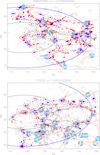 |
Fig. A.1. Plots for visual inspections. Black open circles are galaxies with known velocities within ±1500 km s−1. Large open violet circles represent the position of each group or cluster detected by the FoF algorithm (arbitrary radius). Red filled circles are galaxies in these groups and clusters, but non-virialised. On the other hand, blue filled circles are galaxies in groups that are also virialised and are used to estimate the velocity dispersion and mass. Coral bands are filaments, whereas big, light-blue filled circles are nodes of the cosmic web (both from Chen et al. 2016). The red ellipse is centred at the position of the corresponding FG and has a radius of 5 Mpc at the redshift of the target. Green and blue ellipses are centred in the same position, but their radii are 50 Mpc and 100 Mpc, respectively. |
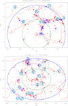 |
Fig. A.1. continued. |
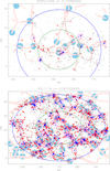 |
Fig. A.1. continued. |
 |
Fig. A.1. continued. |
 |
Fig. A.1. continued. |
 |
Fig. A.1. continued. |
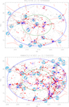 |
Fig. A.1. continued. |
 |
Fig. A.1. continued. |
Appendix B: The large-scale structure of FGS28
In Fig. B.1, we present the large-scale structure around FGS28. As we mention in Sect. 2.2, we did not include this FG into our sample for different reasons. However, since we mention the supercluster and filament that are found very close to FGS28 in both apparent position and redshift, we include this figure for sake of clarity.
 |
Fig. B.1. Large-scale structure around FGS28. Galaxies with SDSS spectroscopy within ±1500 km s−1 from the redshift of FGS28 are represented in black. Moreover, in the bottom-left panel, the large red, green, and blue ellipses represent 5, 50, and 100 Mpc respectively (as in Fig. A.1). The small violet, brown, green, and blue ellipses are the four clusters that are found close to FGS28. In the top-right panel, a zoom can be seen, were the colour coding is the same with the exception of the red ellipse, which now simply identifies the position of FGS28. In this panel, the legend associates each coloured ellipse to a specific clusters. It can be seen that FGS28 is identified by a single galaxy with spectroscopic redshift in SDSS, supporting the notion that this is a isolated galaxy located in the environment of a large supercluster. |
All Tables
All Figures
|
Fig. 1. Spectroscopic completeness for our starting sample. The two systems with completeness smaller than 65% were not included in our final sample. |
| In the text | |
|
Fig. 2. Correlations between Δm12 (top panel), Mr, BCG (middle panel), and LX (lower panel) and the distance to the filament (left column) in units of R200. Same parameters correlated with the distance to the intersections (right column). The dashed horizontal line in the left panel represents 5 R200, which is the distance that we used to separate FGs that are close to filaments (Dfila < 5 R200, blue diamonds) from those that are not (red stars). |
| In the text | |
|
Fig. 3. Comparison between the main general properties of the clusters in our sample. Colour code is the same as in Fig. 2, but here we also show AWM4 as a black dot, since this FG is found at a redshift where the Chen et al. (2016) catalogue is not available and thus it cannot be classified based on its distance to a filament. |
| In the text | |
|
Fig. 4. Cumulative distribution of Δm12 (top left panel), absolute magnitude of the BCG (top right panel), X-ray luminosity (bottom left panel), and R200 (bottom right panel). In each panel, the full FG population is described with the solid black line and black circles, FGs close to filaments are represented with blue dashed line and diamonds, and FGs far from filaments are shown with red dashed-dotted line and stars. |
| In the text | |
|
Fig. 5. Top panel: galaxy over densities for systems with distance to filament larger and smaller than 5 R200 (red open circles and blue filled circles, respectively). Middle panel: same quantities but for systems with bright (Mr < −23) and faint (Mr > −23) central galaxies (green filled diamonds and pink empty diamonds, respectively). Bottom panel: same quantities but for systems with high (LX > 1043) and faint (LX < 1043) X-ray luminosities (azure filled squares and violet open squares, respectively). |
| In the text | |
|
Fig. 6. Correlations between the absolute magnitude of the BCG (top left panel), the magnitude gap (top right panel), the X-ray luminosity (bottom left panel), and redshift (bottom right) vs. the density of galaxies brighter than −22 within 50 Mpc. The area is computed using Pick’s theorem, so footprint incompleteness is properly taken into account. Colour coding and symbols are the same as in Fig. 2. Big open circles represent FGs with central galaxies brighter than −22. |
| In the text | |
|
Fig. 7. Cumulative distribution of bright galaxies (Mr < −22) in 50 Mpc (left panel) and 20 Mpc (right panel). The colour coding is the same as in Fig. 2. |
| In the text | |
|
Fig. 8. Correlations between the mass found by the FoF algorithm within 50 or 100 Mpc (left and right columns, respectively) and some global quantities of our sample. The colour coding is the same as in Fig. 3. |
| In the text | |
|
Fig. A.1. Plots for visual inspections. Black open circles are galaxies with known velocities within ±1500 km s−1. Large open violet circles represent the position of each group or cluster detected by the FoF algorithm (arbitrary radius). Red filled circles are galaxies in these groups and clusters, but non-virialised. On the other hand, blue filled circles are galaxies in groups that are also virialised and are used to estimate the velocity dispersion and mass. Coral bands are filaments, whereas big, light-blue filled circles are nodes of the cosmic web (both from Chen et al. 2016). The red ellipse is centred at the position of the corresponding FG and has a radius of 5 Mpc at the redshift of the target. Green and blue ellipses are centred in the same position, but their radii are 50 Mpc and 100 Mpc, respectively. |
| In the text | |
|
Fig. A.1. continued. |
| In the text | |
|
Fig. A.1. continued. |
| In the text | |
|
Fig. A.1. continued. |
| In the text | |
|
Fig. A.1. continued. |
| In the text | |
|
Fig. A.1. continued. |
| In the text | |
|
Fig. A.1. continued. |
| In the text | |
|
Fig. A.1. continued. |
| In the text | |
|
Fig. B.1. Large-scale structure around FGS28. Galaxies with SDSS spectroscopy within ±1500 km s−1 from the redshift of FGS28 are represented in black. Moreover, in the bottom-left panel, the large red, green, and blue ellipses represent 5, 50, and 100 Mpc respectively (as in Fig. A.1). The small violet, brown, green, and blue ellipses are the four clusters that are found close to FGS28. In the top-right panel, a zoom can be seen, were the colour coding is the same with the exception of the red ellipse, which now simply identifies the position of FGS28. In this panel, the legend associates each coloured ellipse to a specific clusters. It can be seen that FGS28 is identified by a single galaxy with spectroscopic redshift in SDSS, supporting the notion that this is a isolated galaxy located in the environment of a large supercluster. |
| In the text | |
Current usage metrics show cumulative count of Article Views (full-text article views including HTML views, PDF and ePub downloads, according to the available data) and Abstracts Views on Vision4Press platform.
Data correspond to usage on the plateform after 2015. The current usage metrics is available 48-96 hours after online publication and is updated daily on week days.
Initial download of the metrics may take a while.