| Issue |
A&A
Volume 676, August 2023
|
|
|---|---|---|
| Article Number | A133 | |
| Number of page(s) | 6 | |
| Section | Extragalactic astronomy | |
| DOI | https://doi.org/10.1051/0004-6361/202346238 | |
| Published online | 23 August 2023 | |
Fossil group origins
XIII. A paradigm shift: Fossil groups as isolated structures rather than relics of the ancient Universe
1
Instituto de Astrofísica de Canarias, Calle Vía Láctea s/n, 38205 La Laguna, Tenerife, Spain
e-mail: This email address is being protected from spambots. You need JavaScript enabled to view it.
2
Departamento de Astrofísica, Universidad de La Laguna, Avenida Astrofísico Francisco Sánchez s/n, 38206 La Laguna, Spain
3
Dipartimento di Fisica e Astronomia “G. Galilei”, Università di Padova, Vicolo dell’Osservatorio 3, 35122 Padova, Italy
4
INAF-Osservatorio Astronomico di Padova, Vicolo dell’Osservatorio 5, 35122 Padova, Italy
5
Observatorio Astronómico Nacional, IGN, Calle Alfonso XII 3, 28014 Madrid, Spain
Received:
24
February
2023
Accepted:
21
June
2023
Abstract
Aims. In this work we study the large-scale structure around a sample of non-fossil systems and compare the results with earlier findings for a sample of genuine fossil systems selected using their magnitude gap.
Methods. We computed the distance from each system to the closest filament and intersection as obtained from a catalogue of galaxies in the redshift range 0.05 ≤ z ≤ 0.7. We then estimated the average distances and the distributions of cumulative distances to filaments and intersections for different magnitude-gap bins.
Results. We find that the average distance to filaments is (3.0 ± 0.8) R200 for fossil systems, whereas it is (1.1 ± 0.1) R200 for non-fossil systems. Similarly, the average distance to intersections is larger in fossil than in non-fossil systems, with values of (16.3 ± 3.2) and (8.9 ± 1.1) R200, respectively. Moreover, the cumulative distributions of distances to intersections are statistically different for fossil and non-fossil systems.
Conclusions. Fossil systems selected using the magnitude gap appear to be, on average, more isolated from the cosmic web than non-fossil systems. No dependence is found on the magnitude gap (i.e. non-fossil systems behave in a similar manner independently of their magnitude gap, and only fossils are found at larger average distances from the cosmic web). This result supports a formation scenario for fossil systems in which the lack of infalling galaxies from the cosmic web, due to their peculiar position, favours the growing of the magnitude gap via the merging of all the massive satellites with the central galaxy. Comparison with numerical simulations suggests that fossil systems selected using the magnitude gap are not old fossils of the ancient Universe, but rather systems located in regions of the cosmic web not influenced by the presence of intersections.
Key words: galaxies: clusters: general / galaxies: groups: general / large-scale structure of Universe
© The Authors 2023
 Open Access article, published by EDP Sciences, under the terms of the Creative Commons Attribution License (https://creativecommons.org/licenses/by/4.0), which permits unrestricted use, distribution, and reproduction in any medium, provided the original work is properly cited.
This article is published in open access under the Subscribe to Open model. This email address is being protected from spambots. You need JavaScript enabled to view it. to support open access publication.
1. Introduction
Ponman et al. (1994) proposed for the first time the existence of fossil groups (FGs) to explain the discovery of an apparently isolated giant elliptical galaxy, which was surrounded by an extended halo typical of a galaxy group. They supposed that this was the fossil relic of an old group of galaxies, which had had enough time to merge all its bright galaxies into a brightest central galaxy (BCG). To be able to merge all the bright galaxies and create giant isolated BCGs, FGs should be older than regular groups. They were thus proposed as fossil relics of the ancient Universe.
The first observational definition of FGs was given by Jones et al. (2003). They define an FG as a system with a large magnitude gap between the two brightest members (Δm12 > 2 mag in the r band) within half the virial radius of the group. The number of known FGs slowly but steadily grew over the years. Vikhlinin et al. (1999) proposed four candidates defined as “over-luminous red galaxies”, Jones et al. (2003) presented a sample of five FGs, and Santos et al. (2007) presented the first large sample of 34 FG candidates, of which 15 were confirmed as genuine FGs by Zarattini et al. (2014). Miller et al. (2012) and Adami et al. (2018) identified 12 and 18 FGs, respectively, and, more recently, Adami et al. (2020) proposed a new probabilistic method for finding FGs, favouring the statistical study of these systems. Finally, in their review, Aguerri & Zarattini (2021) compile a list of 36 genuine FGs from the literature. For these systems, Δm12 values have been spectroscopically measured and the virial radius properly computed.
However, observational evidence has shown that FGs are not older than non-FGs. For example, the fraction of galaxy substructure in FGs is similar to that of non-FGs (Zarattini et al. 2016), and the stellar age of the central galaxies in FGs is similar to or even less than those in non-FGs (La Barbera et al. 2012; Eigenthaler & Zeilinger 2013; Corsini et al. 2018). In a very recent work, Chu et al. (2023) studied a sample of central galaxies in FG and non-FG candidates, finding that BCGs in FGs should have evolved in a similar way as regular BCGs. This result was also confirmed by their analysis of the stellar populations. They claim that it is currently not possible to find differences in the stellar populations of BCGs in FG and non-FG candidates. In addition, cosmological simulations show that the galaxy aggregations selected as FGs by using the magnitude gap did not form at earlier epochs than non-FGs (Kanagusuku et al. 2016; Kundert et al. 2017). On the other hand, Raouf et al. (2014) suggest that old FGs could be those with large magnitude gaps and small central galaxies.
If FGs are not older than non-FGs, another mechanism is required to explain the increased merging rate of massive satellites in these systems. Sommer-Larsen (2006) propose that a difference in the orbital shape of galaxies in FGs could justify the large magnitude gap, since massive satellites found on more radial orbits merge faster with the BCG. The first observational confirmation of this was made by Zarattini et al. (2021), who measured the dependence of the anisotropy parameter on Δm12. They show that systems with Δm12 < 1.5 mag are characterised by isotropic orbits (e.g. galaxies are equally distributed on radial and tangential orbits), whereas systems with Δm12 > 1.5 mag have a larger fraction of galaxies on radial orbits, especially in the external regions, within 0.7 − 1 R200.
The location of FGs in the large-scale structure could also play an important role in our understanding of these systems, but few studies have been devoted to this topic. Adami et al. (2012, 2018) studied two FGs and one non-FG using different approaches, finding that FGs are found in less dense large-scale environments with respect to the control group. More recently, Zarattini et al. (2022) analysed the large-scale structure around a sample of 16 FGs. They are found close to filaments, with an average distance of (3.7 ± 1.1) R200 and a minimum distance of 0.05 R200, and far from intersections, with an average distance of (19.3 ± 3.6) R200 and a minimum distance of 6.1 R200.
The goal of this paper is to analyse how these distances compare to those of non-FGs. Here, we consider a sample of 55 clusters and groups with Δm12 < 2 mag, and we compare its properties with those of the 16 FGs analysed by Zarattini et al. (2022). This work is part of the Fossil Group Origins (FOGO) project (Aguerri et al. 2011), a large observational effort aimed at characterising the properties of the sample of 34 FG candidates presented in Santos et al. (2007).
The cosmic web description that we use in this work comes from Chen et al. (2015, 2016). The detection is based on the subspace constrained mean shift (SCMS) algorithm. The SCMS algorithm is a gradient ascent method that models filaments as density ridges, one-dimensional smooth curves that trace high-density regions within the point cloud. The algorithm consists of three steps (see Chen et al. 2015, for a detailed description of the formalism): the first step is estimating the underlying density function given the observed location of galaxies using the standard kernel density estimator. The second step is the de-noising of the estimated density function, which is needed to eliminate the effect that galaxies in low-probability density regions would have on filament estimations. This step is crucial to increasing the statistical power of the SCMS algorithm in low-density regions. The third and final step is the application of the original SCMS algorithm (Ozertem & Erdogmus 2011) to galaxies in high-density regions. Chen et al. (2016) applied this method to a simulated dataset based on the Voronoi model (van de Weygaert 1994), showing that the SCMS algorithm reproduces clusters, filaments, and walls in a precise way. The SCMS algorithm was then applied in Chen et al. (2016) to Sloan Digital Sky Survey (SDSS) DR7 and DR12 data to produce the final catalogue of filaments and intersections that we use in this work. The main disadvantage of this method is that the coverage depends sensitively on the number of galaxies in the analysed sample. This could be an issue since SDSS spans a large area and the coverage cannot be homogeneous in the full footprint and in the entire redshift range. For example, a well-known issue affecting SDSS is that the selection function for the spectroscopic follow-up is split into two parts (see Fig. 3 of Tarrío & Zarattini 2020): one peaked at redshifts z ∼ 0.1 and one peaked at redshift z ∼ 0.5, with a clear lack of redshifts in the range 0.2 < z < 0.4.
The cosmology adopted in this paper, as well as in the other FOGO papers, is H0 = 70 km s−1 Mpc−1, Ωm = 0.3, and ΩΛ = 0.7. We use RΔ to denote the radius of a sphere within which the average mass density is Δ times the critical density of the Universe at the redshift of the galaxy system; θΔ is the corresponding angular radius, and MΔ is the mass contained in RΔ.
2. Sample
Zarattini et al. (2022) present an analysis of the large-scale environment of a sample of genuine FGs. This sample consists of the 16 FGs in the redshift range 0.03 < z < 0.15 discussed by Aguerri & Zarattini (2021). However, one of the FGs, namely AWM4, was found at z < 0.05, which is the limit of the Chen et al. (2016) filament and intersection catalogue used in Zarattini et al. (2022) and in this work. We thus removed AWM4 from the sample, which left us with 15 genuine FGs.
The goal of this paper is to compare the properties of the FGs discussed in Zarattini et al. (2022) with those of a sample of non-FGs that span similar ranges in redshift and mass. The non-FG systems are taken from Aguerri et al. (2007). In particular, we used all the systems with a spectroscopically confirmed magnitude gap in the redshift range 0.05 < z < 0.15 and with Δm12 < 2.0 mag. The total number of these systems is 55.
The magnitude gap distribution of FGs and non-FGs is shown in the first panel of Fig. 1. Most systems have small magnitude gaps, with a near absence of systems in the range 1.5 < Δm12 < 2.0 mag.
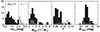 |
Fig. 1. Properties of the sample systems. From left to right: magnitude gap distribution, total mass distribution, redshift distribution, and distribution of the absolute magnitude of the BCGs. The FGs from Zarattini et al. (2022) are shown in violet, while the non-FGs are shown in black. |
The mass distribution of the two samples is shown in the second panel of Fig. 1. The mass was obtained by filtering X-ray maps from the ROSAT All-Sky Survey (RASS; Truemper 1993; Voges et al. 1999) with the X-ray-matched filter described in Tarrío et al. (2016, 2018), which assumes the average gas density profile from Piffaretti et al. (2011). We used the filter in fixed-position and blind-size modes, that is, centered at the position of the object (with a small margin to search for the X-ray peak), and using 32 different sizes covering θ500 from  to
to  . The output of the filter is a flux-size degeneracy curve, which provides the X-ray flux of the object within R500 in the [0.1−2.4] KeV band (FX) for the different values of θ500. The mass was then obtained by computing the Sunyaev–Zel’dovich flux of the cluster within R500 (Y500) using the FX/Y500 relation found by Planck Collaboration Int. I (2012) at the cluster redshift, and breaking the flux-size degeneracy with the
  1 scaling relation from Planck Collaboration XX (2014), which relates θ500 and Y500 when z is known, as explained in Planck Collaboration XXIX (2014) and Tarrío et al. (2018). The mass distributions of FGs and non-FGs are similar to each other, although in the FG sample we are missing the very low-mass end of the distribution (M500 < 3 × 10¹³ M⊙). A Kolmogorov–Smirnov (KS) test confirms that the two distributions come from the same parent distribution (pM500 = 0.99).
From the same analysis, we also estimated the R500 radii for both samples. This was done in order to have homogeneous measurements, since some of the radii available in the literature were computed from X-rays and others from the velocity dispersion of galaxies. We then converted the R500 to R200 using R200 = 1.516 × R500 (Arnaud et al. 2005). The median values of R200 are (1.1 ± 0.2) Mpc and (1.1 ± 0.3) Mpc for fossils and non-fossils, respectively.
The redshift distribution of the two samples is presented in the third panel of Fig. 1. On average, FGs are found at a slightly higher redshift. However, this is not an issue since the median redshifts are 0.08 ± 0.02 and 0.12 ± 0.03 for non-FGs and FGs, respectively. This corresponds to an age difference of about 0.5 Gyr, for which we do not expect any evolution effect since it is a relatively short timescale. In this case, the KS test confirms the difference between the two redshift distributions (pz = 0.0015).
Finally, in the fourth panel of Fig. 1 we show the distribution of the absolute magnitude of the BCGs for FGs and non-FGs. In this case, non-FGs show a clear peak at about Mr = −23 mag, whereas FGs show a double peak at about Mr = −22.5 and Mr = −23.5 mag. The KS test confirms the difference between the two distributions (pMr = 0.039).
3. Results
Following Zarattini et al. (2022), we computed the distance from each system to the cosmic web filaments and intersections listed in the Chen et al. (2016) catalogue. They are identified using SDSS data in combination with the SCMS algorithm (Chen et al. 2015, and references therein). In particular, SCMS performs a three-step analysis (density estimation, thresholding, and gradient ascent) to detect filaments and intersections. The catalogue uses galaxies with spectroscopic redshifts in the range 0.05 < z < 0.7.
In Fig. 2 we present the distances of our sample of 55 non-FGs combined with the 15 FGs analysed in Zarattini et al. (2022) to filaments (top panel) and intersections (bottom panel) as a function of Δm12. It is worth noting that we also recomputed the distances to filaments and intersections for the sample of FGs. This is due to the choice of deriving R200 in a homogeneous way for all the analysed systems.
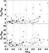 |
Fig. 2. Minimum distance to the filaments (top panel) and intersections (bottom panel) as a function of the magnitude gap. The larger symbols correspond to the average values of the different magnitude gap intervals as listed in Table 1. The horizontal dashed line in both panels indicates the distance of 4 R200. |
Non-FGs show a more compact distribution, especially when analysing the distribution of the distances to filaments, with only one of them having a filament at more than 4 R200 (< 2%). On the other hand, 5 out of the 15 FGs have filaments at a distance greater than 4 R200 (31%). This can suggest a sort of bimodality for FGs. To test this scenario, we applied a kernel mixture model test (KMM, Ashman et al. 1994) to the data, finding that the bimodality is confirmed (the null hypothesis is rejected with a p-value of 0.005, and the two peaks are found at 1.1 and 6.7 R200). However, Ashman et al. (1994) claimed that using small datasets could lead to unreliable conclusions on the bimodality, and in this case the number of elements used to run the KMM test was 15.
We report the average distances from filaments as a function of Δm12 in the second column of Table 1. It can be seen that, if we compare the average values for FGs and non-FGs (0.0 ≤ Δm12 < 2.0), the difference is significant at more than the 2σ level. We also ran a test to compute the Student’s T-statistic and the probability that two distributions have significantly different averages (t-test). The probability is pfila, ave = 0.0002, confirming that the two distributions have different averages.
Average distances to filaments and intersections, and their uncertainties, for different magnitude gaps.
A similar result is found for the distance to intersections of the cosmic web. These distances are shown in Table 1 as well. The distance to intersections is always larger than that to filaments in all the magnitude-gap bins. This is expected since different filaments converge to a single intersection, and so a cluster is more likely to be close to a filament than to an intersection. Moreover, Chen et al. (2016) also define filaments within intersections, so there is always at least one filament at any intersection position. Again, the distances to intersections for non-FGs are systematically smaller than for FGs, and no FG has a distance of less than 4 R200 to the closest intersection. On the other hand, the smallest distances for the four non-FG bins of growing magnitude gaps are 1.2, 1.2, 2.9, and 0.5 R200. We also ran the t-test for the two distributions of distances for FGs and non-FGs, finding pint, ave = 0.007, which again confirms that these distributions have different averages.
We also computed the cumulative fraction of the distance to filaments and intersections for non-FGs in the four bins of Δm12 and for the FGs. The results are shown in Fig. 3. The behaviour of FGs is different from that of non-FGs. We used the KS test to check if the differences are statistically significant. For filaments, the distribution of FGs is not different from that of any of the non-FG bins. The result of the KS test between FGs and non-FGs is pfila = 0.083. If we remove the only non-FG that is found with a filament at more than 4 R200, the KS probability drops to pfila = 0.060. This is still not a significant difference, but the parameter is closer to the threshold. This result could be related to the observed bimodality in the distance to the filament distribution for FGs. The fact that about two-thirds of them are found close to filaments and one-third are at more than 4 R200 could justify the insignificant difference in this parameter. On the other hand, the difference in the distributions of the distance to intersections is statistically significant, with pint = 0.013.
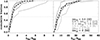 |
Fig. 3. Cumulative distributions of distances from filaments (left panel) and intersections (right panel). Blue lines mark the systems with Δm12 < 0.5 mag, red lines systems with 0.5 ≤ Δm12 < 1.0 mag, green lines systems with 1.0 ≤ Δm12 < 1.5 mag, and orange lines systems with 1.5 ≤ Δm12 < 2.0 mag. In both panels, the dashed black line is the cumulative distribution for all non-FG systems (Δm12 < 2.0), while the violet line corresponds to FGs (Δm12 ≥ 2.0 mag). The numbers within parentheses indicate the size of the samples for each cumulative function. The horizontal dashed line indicates the 50 percentile of the distributions. |
4. Discussion and conclusions
In Fig. 1 we show the mass distribution of FGs and non-FGs. The distributions are quite similar, but we also computed the cumulative distribution of distances after removing the most extreme systems from both samples. In particular, we repeated the computation using only objects in the mass range 1013 ≤ M500 ≤ 2.5 × 10¹⁴ M⊙. The results remain unchanged, the distance distribution from intersections being statistically different between FGs and non-FGs (p*int = 0.026). No differences are found for filaments (pfila = 0.14).
Our results can be interpreted in terms of the formation scenario of FGs. Ponman et al. (1994) claimed that FGs were able to build large magnitude gaps thanks to their isolation from the cosmic web. Indeed, in this work we show that FGs are systematically more isolated than non-FGs. In particular, the average distance to filaments and intersections is larger for FGs than non-FGs. The distance to intersections is of particular interest since intersections are considered to be the places in the cosmic web where the mass accretion is more efficient and where galaxy clusters are supposed to live. However, we are now showing that this distance is statistically different for FGs and non-FGs, FGs being systematically farther from intersections than non-FGs.
Kraljic et al. (2018) show that filament galaxies at more than 3.5 Mpc from the centre of an intersection are not influenced (or are only marginally influenced) by the intersection itself. This measure is used for isolated galaxies and not for groups or clusters. However, we speculate that the larger distance that separates FGs from intersections can have an impact on their mass-accretion process (e.g. a smaller number of galaxies could be accreted far from intersections). It is important to keep in mind that we are computing distances from the centres of filaments and intersections, the sizes of which Chen et al. (2016) did not estimate. Thus, it is difficult to say, with the available data, if our FGs are really outside filaments and intersections. We can only claim that FGs are systematically farther than non-FGs in both cases.
In Cossairt et al. (2022) the large-scale structure around FG and non-FG candidates was studied using a gravity-only cosmological simulation. The authors find that there is no statistical difference in the environments in which FGs and non-FGs formed. However, it is worth noting that the method for selecting FGs in Cossairt et al. (2022) is deeply different from ours. In particular, we used the observational definition based on the magnitude gap, which they did not use; their selection is based on the idea that FGs are old systems that have not experienced major mergers in recent times. However, this idea does not properly describe the optically selected FGs. In fact, it has been shown that systems selected from the magnitude gap are not particularly old, that their BCGs have similar stellar populations as non-FGs (La Barbera et al. 2009; Eigenthaler & Zeilinger 2013; Corsini et al. 2018; Chu et al. 2023), that their fraction of substructure is similar to that of non-FGs (Zarattini et al. 2016), and that the gap is very recent (Kundert et al. 2017). For optically selected FG, Jones et al. (2003) and Adami et al. (2018, 2020) find hints of a different large-scale environment, with FGs being more isolated (e.g. in a less dense environment), a result that we now confirm with a statistically significant sample. We thus think that a direct comparison between optically selected FGs and those from the Cossairt et al. (2022) simulations is not straightforward due to the very different selection functions. Indeed, the latter systems are probably more connected to the original idea of what an FG was expected to be. Nevertheless, we can learn a lot from this difference. In particular, we can now say that the comparison between observational findings and simulation results calls for the definition of FGs itself to be changed: systems selected with a large magnitude gap at z = 0 are not old fossils of the ancient Universe; they are instead isolated systems with a peculiar position in the cosmic web. This location reduces the number of major accretion events in recent epochs and connects the formation of the magnitude gap to the internal evolution of these systems, with their high merging rate supported by more radial orbits (Zarattini et al. 2021). On the other hand, Cossairt et al. (2022) show that systems selected to be old and relaxed are not in a peculiar location in the cosmic web, and they have to be selected with a different diagnostic than the magnitude gap. Indeed, Kundert et al. (2017) studied a sample of FGs selected in the Illustris cosmological simulations for having Δm12 > 2.0 mag at z = 0, and they compared the halo mass assembly at early times for these FGs with a sample of non-FGs, finding no differences in their formation times. This result confirmed that the magnitude gap is not the proper parameter to use to select old systems.
In a very recent work, Taverna et al. (2023) analysed the large-scale structure around a sample of Hickson-like compact groups. These systems were claimed to be the precursors of FGs (Barnes 1989; Vikhlinin et al. 1999; Jones et al. 2003). It would thus be interesting to determine whether the position of FGs and compact groups in the cosmic web is similar or not. Taverna et al. (2023) define four different environments: (i) nodes of filaments, (ii) loose groups, (iii) filaments, and (iv) cosmic voids. They claim that 45% of compact groups do not reside in any of these structures. This result seems to be in good agreement with our findings, although, as already mentioned, we are not able to define whether our systems are inside a filament or an intersection. However, we do find that FGs are systematically farther from both types of structures. So, according to these results, a link between FGs and compact groups cannot be excluded (but see also Mendes de Oliveira & Carrasco 2007).
Our conclusions can be summarised as follows:
-
We compared a sample of FGs taken from Aguerri & Zarattini (2021) with a sample of 55 non-FGs taken from Aguerri et al. (2007). The two samples have similar mass ranges. Their redshift distributions are not identical, but the difference corresponds to about 0.5 Gyr and is not significant in terms of cluster evolution.
-
Fossil groups are more isolated from the cosmic web than non-FGs. In fact, the average distances to filaments and intersections for the former are (3.0 ± 0.8) R200 and (16.3 ± 3.2) R200, respectively. For comparison, the average distances for the latter are (1.1 ± 0.1) R200 and (8.9 ± 1.1) R200, respectively. These results remain qualitatively unchanged if we remove the most extreme systems in terms of mass. A t-test confirms that the two distributions have different averages.
-
The cumulative distribution of the distances to intersections for FGs and non-FGs is also found to be different, with the former found at greater distances. The statistical significance of the result was confirmed with a KS test.
-
For non-FGs, the distance to filaments and intersections does not seem to depend on the magnitude gap. The difference arises only for systems with Δm12 ≥ 2 mag.
-
We can thus conclude that FGs are in a peculiar position of the cosmic web, being more isolated than non-FGs. This result is in agreement with previous observational works (Jones et al. 2003; Adami et al. 2018, 2020) but not with the gravity-only simulations by Cossairt et al. (2022). The most probable reason for this disagreement is the different selection function of FGs in observations (based on the magnitude gap at z = 0) and simulations (lack of massive halo mergers since z = 1).
Our interpretation of this tension between observations and simulations is that FGs selected with Δm12 > 2 mag at z = 0 are not old fossils of the ancient Universe, but rather systems isolated from the cosmic web. The formation of the large magnitude gap would then be related more to internal processes (e.g. the predominance of radial orbits; Zarattini et al. 2021) than to an early formation epoch.
DA is the angular size distance to the galaxy system.
Acknowledgments
We thank the referee for his/her constructive comments that improved the clarity and the quality of the paper. We also would like to thank Marisa Girardi for useful discussions about the KMM test. S.Z. is supported by the Ministry of Science and Innovation of Spain, projects PID2019-107408GB-C43 (ESTALLIDOS) and PID2020-119342GB-I00, by the Government of the Canary Islands through EU FEDER funding project PID2021010077. S.Z. and E.M.C. are supported by MIUR grant PRIN 2017 20173ML3WW-001 and Padua University grants DOR2019-2021. J.A.L.A. is supported by the grant PID2020-119342GB-I00.
References
- Adami, C., Jouvel, S., Guennou, L., et al. 2012, A&A, 540, A105 [NASA ADS] [CrossRef] [EDP Sciences] [Google Scholar]
- Adami, C., Giles, P., Koulouridis, E., et al. 2018, A&A, 620, A5 [NASA ADS] [CrossRef] [EDP Sciences] [Google Scholar]
- Adami, C., Sarron, F., Martinet, N., & Durret, F. 2020, A&A, 639, A97 [NASA ADS] [CrossRef] [EDP Sciences] [Google Scholar]
- Aguerri, J. A. L., & Zarattini, S. 2021, Universe, 7, 132 [NASA ADS] [CrossRef] [Google Scholar]
- Aguerri, J. A. L., Sánchez-Janssen, R., & Muñoz-Tuñón, C. 2007, A&A, 471, 17 [NASA ADS] [CrossRef] [EDP Sciences] [Google Scholar]
- Aguerri, J. A. L., Girardi, M., Boschin, W., et al. 2011, A&A, 527, A143 [NASA ADS] [CrossRef] [EDP Sciences] [Google Scholar]
- Arnaud, M., Pointecouteau, E., & Pratt, G. W. 2005, A&A, 441, 893 [NASA ADS] [CrossRef] [EDP Sciences] [Google Scholar]
- Ashman, K. M., Bird, C. M., & Zepf, S. E. 1994, AJ, 108, 2348 [Google Scholar]
- Barnes, J. E. 1989, Nature, 338, 123 [NASA ADS] [CrossRef] [Google Scholar]
- Chen, Y.-C., Ho, S., Tenneti, A., et al. 2015, MNRAS, 454, 3341 [NASA ADS] [CrossRef] [Google Scholar]
- Chen, Y.-C., Ho, S., Brinkmann, J., et al. 2016, MNRAS, 461, 3896 [NASA ADS] [CrossRef] [Google Scholar]
- Chu, A., Durret, F., Ellien, A., et al. 2023, A&A, 673, A100 [NASA ADS] [CrossRef] [EDP Sciences] [Google Scholar]
- Corsini, E. M., Morelli, L., Zarattini, S., et al. 2018, A&A, 618, A172 [NASA ADS] [CrossRef] [EDP Sciences] [Google Scholar]
- Cossairt, A., Buehlmann, M., Kovacs, E., et al. 2022, Open J. Astrophys., 5 [Google Scholar]
- Eigenthaler, P., & Zeilinger, W. W. 2013, A&A, 553, A99 [NASA ADS] [CrossRef] [EDP Sciences] [Google Scholar]
- Jones, L. R., Ponman, T. J., Horton, A., et al. 2003, MNRAS, 343, 627 [NASA ADS] [CrossRef] [Google Scholar]
- Kanagusuku, M. J., Díaz-Giménez, E., & Zandivarez, A. 2016, A&A, 586, A40 [NASA ADS] [CrossRef] [EDP Sciences] [Google Scholar]
- Kraljic, K., Arnouts, S., Pichon, C., et al. 2018, MNRAS, 474, 547 [Google Scholar]
- Kundert, A., D’Onghia, E., & Aguerri, J. A. L. 2017, ApJ, 845, 45 [NASA ADS] [CrossRef] [Google Scholar]
- La Barbera, F., de Carvalho, R. R., de la Rosa, I. G., et al. 2009, AJ, 137, 3942 [NASA ADS] [CrossRef] [Google Scholar]
- La Barbera, F., Paolillo, M., De Filippis, E., & de Carvalho, R. R. 2012, MNRAS, 422, 3010 [CrossRef] [Google Scholar]
- Mendes de Oliveira, C. L., & Carrasco, E. R. 2007, ApJ, 670, L93 [CrossRef] [Google Scholar]
- Miller, E. D., Rykoff, E. S., Dupke, R. A., et al. 2012, ApJ, 747, 94 [NASA ADS] [CrossRef] [Google Scholar]
- Ozertem, U., & Erdogmus, D. 2011, J. Mach. Learn. Res., 12, 1249 [Google Scholar]
- Piffaretti, R., Arnaud, M., Pratt, G. W., Pointecouteau, E., & Melin, J. B. 2011, A&A, 534, A109 [NASA ADS] [CrossRef] [EDP Sciences] [Google Scholar]
- Planck Collaboration XX. 2014, A&A, 571, A20 [NASA ADS] [CrossRef] [EDP Sciences] [Google Scholar]
- Planck Collaboration XXIX. 2014, A&A, 571, A29 [NASA ADS] [CrossRef] [EDP Sciences] [Google Scholar]
- Planck Collaboration Int. I. 2012, A&A, 543, A102 [NASA ADS] [CrossRef] [EDP Sciences] [Google Scholar]
- Ponman, T. J., Allan, D. J., Jones, L. R., et al. 1994, Nature, 369, 462 [Google Scholar]
- Raouf, M., Khosroshahi, H. G., Ponman, T. J., et al. 2014, MNRAS, 442, 1578 [NASA ADS] [CrossRef] [Google Scholar]
- Santos, W. A., Mendes de Oliveira, C., & Sodré, L., Jr. 2007, AJ, 134, 1551 [NASA ADS] [CrossRef] [Google Scholar]
- Sommer-Larsen, J. 2006, MNRAS, 369, 958 [Google Scholar]
- Tarrío, P., & Zarattini, S. 2020, A&A, 642, A102 [NASA ADS] [CrossRef] [EDP Sciences] [Google Scholar]
- Tarrío, P., Melin, J. B., Arnaud, M., & Pratt, G. W. 2016, A&A, 591, A39 [NASA ADS] [CrossRef] [EDP Sciences] [Google Scholar]
- Tarrío, P., Melin, J. B., & Arnaud, M. 2018, A&A, 614, A82 [NASA ADS] [CrossRef] [EDP Sciences] [Google Scholar]
- Taverna, A., Salerno, J. M., Daza-Perilla, I. V., et al. 2023, MNRAS, 520, 6367 [CrossRef] [Google Scholar]
- Truemper, J. 1993, Science, 260, 1769 [Google Scholar]
- van de Weygaert, R. 1994, A&A, 283, 361 [NASA ADS] [Google Scholar]
- Vikhlinin, A., McNamara, B. R., Hornstrup, A., et al. 1999, ApJ, 520, L1 [NASA ADS] [CrossRef] [Google Scholar]
- Voges, W., Aschenbach, B., Boller, T., et al. 1999, A&A, 349, 389 [NASA ADS] [Google Scholar]
- Zarattini, S., Barrena, R., Girardi, M., et al. 2014, A&A, 565, A116 [NASA ADS] [CrossRef] [EDP Sciences] [Google Scholar]
- Zarattini, S., Girardi, M., Aguerri, J. A. L., et al. 2016, A&A, 586, A63 [NASA ADS] [CrossRef] [EDP Sciences] [Google Scholar]
- Zarattini, S., Biviano, A., Aguerri, J. A. L., Girardi, M., & D’Onghia, E. 2021, A&A, 655, A103 [NASA ADS] [CrossRef] [EDP Sciences] [Google Scholar]
- Zarattini, S., Aguerri, J. A. L., Calvi, R., & Girardi, M. 2022, A&A, 668, A38 [NASA ADS] [CrossRef] [EDP Sciences] [Google Scholar]
All Tables
Average distances to filaments and intersections, and their uncertainties, for different magnitude gaps.
All Figures
|
Fig. 1. Properties of the sample systems. From left to right: magnitude gap distribution, total mass distribution, redshift distribution, and distribution of the absolute magnitude of the BCGs. The FGs from Zarattini et al. (2022) are shown in violet, while the non-FGs are shown in black. |
| In the text | |
|
Fig. 2. Minimum distance to the filaments (top panel) and intersections (bottom panel) as a function of the magnitude gap. The larger symbols correspond to the average values of the different magnitude gap intervals as listed in Table 1. The horizontal dashed line in both panels indicates the distance of 4 R200. |
| In the text | |
|
Fig. 3. Cumulative distributions of distances from filaments (left panel) and intersections (right panel). Blue lines mark the systems with Δm12 < 0.5 mag, red lines systems with 0.5 ≤ Δm12 < 1.0 mag, green lines systems with 1.0 ≤ Δm12 < 1.5 mag, and orange lines systems with 1.5 ≤ Δm12 < 2.0 mag. In both panels, the dashed black line is the cumulative distribution for all non-FG systems (Δm12 < 2.0), while the violet line corresponds to FGs (Δm12 ≥ 2.0 mag). The numbers within parentheses indicate the size of the samples for each cumulative function. The horizontal dashed line indicates the 50 percentile of the distributions. |
| In the text | |
Current usage metrics show cumulative count of Article Views (full-text article views including HTML views, PDF and ePub downloads, according to the available data) and Abstracts Views on Vision4Press platform.
Data correspond to usage on the plateform after 2015. The current usage metrics is available 48-96 hours after online publication and is updated daily on week days.
Initial download of the metrics may take a while.