| Issue |
A&A
Volume 665, September 2022
|
|
|---|---|---|
| Article Number | A93 | |
| Number of page(s) | 13 | |
| Section | Extragalactic astronomy | |
| DOI | https://doi.org/10.1051/0004-6361/202244075 | |
| Published online | 15 September 2022 | |
Detection of an unidentified soft X-ray emission feature in NGC 5548
1
SRON Netherlands Institute for Space Research, Niels Bohrweg 4, 2333 CA Leiden, The Netherlands
e-mail: This email address is being protected from spambots. You need JavaScript enabled to view it.
2
RIKEN High Energy Astrophysics Laboratory, 2-1 Hirosawa, Wako, Saitama 351-0198, Japan
3
Leiden Observatory, Leiden University, PO Box 9513, 2300 RA Leiden, The Netherlands
4
Department of Astronomy, Tsinghua University, Beijing 100084, PR China
5
Department of Physics, Hiroshima University, 1-3-1 Kagamiyama, Higashi Hiroshima, Hiroshima 739-8526, Japan
6
Department of Physics, University of Strathclyde, Glasgow G4 0NG, UK
7
Space Telescope Science Institute, 3700 San Martin Drive, Baltimore, MD 21218, USA
8
INAF – IASF Palermo, via U. La Malfa 153, 90146 Palermo, Italy
9
ESTEC/ESA, Keplerlaan 1, 2201 AZ Noordwijk, The Netherlands
10
Mullard Space Science Laboratory, University College London, Holmbury St. Mary, Dorking, Surrey RH5 6NT, UK
11
Dipartimento di Matematica e Fisica, Universitá degli Studi Roma Tre, via della Vasca Navale 84, 00146 Roma, Italy
12
Centre for Extragalactic Astronomy, Department of Physics, Durham University, South Road, Durham DH1 3LE, UK
13
Mullard Space Science Laboratory, University College London, Holmbury St Mary, Dorking, Surrey RH5 6NT, UK
14
Telespazio UK for the European Space Agency (ESA), European Space Astronomy Centre (ESAC), Camino Bajo del Castillo, s/n, 28692 Villanueva de la Cañada, Madrid, Spain
15
Univ. Grenoble Alpes, CNRS, IPAG, 38000 Grenoble, France
16
Department of Physics, Technion, Haifa, Israel
17
Italian Space Agency (ASI), Via del Politecnico snc, 00133 Roma, Italy
18
Departament de Física, EEBE, Universitat Politécnica de Catalunya, Av. Eduard Maristany 16, 08019 Barcelona, Spain
Received:
20
May
2022
Accepted:
16
July
2022
Abstract
Context. NGC 5548 is an X-ray bright Seyfert 1 active galaxy. It exhibits a variety of spectroscopic features in the soft X-ray band, in particular including the absorption by the active galactic nucleus (AGN) outflows of a broad range of ionization states, with column densities up to 1027 m−2, and having speeds up to several thousand kilometers per second. The known emission features are in broad agreement with photoionized X-ray narrow and broad emission line models.
Aims. We report on an X-ray spectroscopic study using 1.1 Ms XMM-Newton and 0.9 Ms Chandra grating observations of NGC 5548 spanning two decades. The aim is to search and characterize any potential spectroscopic features in addition to the known primary spectral components that are already modeled in high precision.
Methods. For each observation, we modeled the data using a global fit including an intrinsic spectral energy distribution of the AGNs and the known distant X-ray absorbers and emitters. We utilized as much knowledge from previous studies as possible. The fit residuals were stacked and scanned for possible secondary features.
Results. We detect a weak unidentified excess emission feature at ∼18.4 Å (18.1 Å in the restframe). The feature is seen at > 5σ statistical significance taking the look-elsewhere effect into account. No known instrumental issues, atomic transitions, or astrophysical effects can explain this excess. The observed intensity of the possible feature seems to anticorrelate in time with the hardness ratio of the source. However, even though the variability might not be intrinsic, it might be caused by the time-variable obscuration by the outflows. An intriguing possibility is the line emission from charge exchange between a partially ionized outflow and a neutral layer in the same outflow, or in the close environment. Other possibilities, such as emission from a highly ionized component with high outflowing speed, cannot be fully ruled out.
Key words: X-rays: galaxies / galaxies: active / galaxies: Seyfert / galaxies: individual: NGC 5548 / atomic processes
© L. Gu et al. 2022
 Open Access article, published by EDP Sciences, under the terms of the Creative Commons Attribution License (https://creativecommons.org/licenses/by/4.0), which permits unrestricted use, distribution, and reproduction in any medium, provided the original work is properly cited.
This article is published in open access under the Subscribe-to-Open model. This email address is being protected from spambots. You need JavaScript enabled to view it. to support open access publication.
1. Introduction
High resolution X-ray spectra of active galactic nuclei (AGNs) provide a powerful tool to study the physical condition of matter in the proximity of the supermassive black hole (Turner & Miller 2009; Reynolds 2016). These materials are thought to be photoionized by the strong radiation field from the inner central engine (e.g., Kaastra et al. 2012). Complicated absorption lines and edges have been discovered for more than 50% of the Seyfert 1 galaxies (Crenshaw et al. 2003; McKernan et al. 2007; Longinotti et al. 2010), suggesting line-of-sight outflow velocities of 100–1000 km s−1 and column densities of 1024 − 1027 m−2, otherwise known as “warm absorbers”. Photoionized gas components outside the line of sight are found to be responsible for broad and narrow emission lines, as well as the narrow radiative recombination continuum observed in soft X-rays (Kaastra et al. 2000; Costantini et al. 2007; Guainazzi & Bianchi 2007; Whewell et al. 2015; Mao et al. 2018, 2019; Grafton-Waters et al. 2020, 2021). Obscuration of the soft X-ray continuum and extreme-ultraviolet (EUV) emission by outflowing gas with a high velocity (> 1000 km s−1), relatively high column density (> 1026 m−2), and low ionization states have recently been reported for a few AGNs (Kaastra et al. 2014). Furthermore, resonance absorption lines in the Fe-K band with higher velocity shifts have been detected in several radio-quiet sources, indicating outflows at a quasi-relativistic velocity ∼0.1c (Tombesi et al. 2010; Parker et al. 2017; Pinto et al. 2018; Kosec et al. 2018a; Reeves et al. 2020).
Apart from the above spectroscopic features, there have been claims of various secondary components in the AGN spectra. Despite being relatively uncertain, these possible weak features might add new insights to the physical picture of active galaxies. For instance, Pounds et al. (2018) reported the detection of redshifted absorption lines of ionized Fe, Ca, Ar, S, and Si with the XMM-Newton spectra of PG1211+143, suggesting an inflow of matter with a velocity of 0.3c onto the black hole. A similar weak feature was reported by Giustini et al. (2017) with the spectra of NGC 2617. Using the XMM-Newton reflection grating spectrometer (RGS) data of 1H0707-495, Blustin & Fabian (2009) claimed weak broad emission lines from C, N, O, and Fe showing both redshifted and blueshifted wings, which were interpreted as a part of the reflection line emission component from the accretion disk. In a subsequent work, Kosec et al. (2018a) showed that the blueshifted component becomes more significant as new observations are added, while the redshifted part is less certain as the significance remains low with the new data. There are also hints of weak transitions from highly excited states of N VII and S XV detected with X-ray and UV spectroscopy, which might originate from charge exchange between the ionized AGN outflows and the neutral environmental materials (Gu et al. 2017; Mao et al. 2018). Since many of these discoveries have been made at the limits of the available data, it is often difficult to fully address the uncertainties of the claimed line detection (Vaughan & Uttley 2008).
The archetypal Seyfert 1 galaxy NGC 5548 is one of the most extensively studied AGNs (Kaastra et al. 2000, 2014; Bottorff et al. 2000; Mehdipour et al. 2015; Cappi et al. 2016; Goad et al. 2016; Dehghanian et al. 2019a,b; Landt et al. 2015, 2019; Kriss et al. 2019; Wildy et al. 2021). It is arguably one of best active galaxies for the weak feature search for the following two reasons: (1) the available XMM-Newton and Chandra grating data of this object have accumulated to > 2 Ms in total, making it one of the deepest spectroscopic AGN datasets so far; and (2) the primary spectral components have been modeled to good precision in previous works. It was the first target in which narrow X-ray absorption lines from warm absorbers were discovered (Kaastra et al. 2000). These absorbers are continuously studied for spectral and temporal properties (Steenbrugge et al. 2005; Di Gesu et al. 2015; Ebrero et al. 2016). The deep multiwavelength campaign of NGC 5548 during the obscuration phase in 2013−2014 provided unprecedented constraints on the ionization states, column densities, and kinematics of the obscurers (Kaastra et al. 2014; Mehdipour et al. 2015). The heavily obscured state further offers a unique opportunity to accurately model the narrow emission lines and radiative recombination continua, which stand out at a low continuum level (Steenbrugge et al. 2005; Detmers et al. 2009; Whewell et al. 2015; Mao et al. 2018).
For this work we performed a systematic search for weak spectral components in the NGC 5548 spectra in the soft X-ray band by reanalyzing all the available XMM-Newton RGS and Chandra low-energy transmission grating spectrometer (LETGS) data, based on the accumulated knowledge on the primary spectral components. The structure of the paper is as follows. Section 2 provides information on the data processing, spectral modeling, line detection, and the analysis of systematic uncertainties. In Sect. 3, we discuss the possible interpretation of the new emission feature detected. All errors quoted throughout the paper correspond to a 68% confidence level. The redshift of NGC 5548 is set to 0.017175 (de Vaucouleurs et al. 1991).
2. Analysis and results
2.1. Observations and data reduction
We use a total of ten Chandra and 19 XMM-Newton archival observations. For some observations, the data were taken in a (quasi-)consecutive period with the same instrumental setting. We combined such data together for better statistics. Table 1 shows the observation log.
NGC 5548 archival observation log.
The XMM-Newton RGS data were used in combination with the European Photon Imaging Camera (EPIC) pn data. The RGS instruments were operated in the standard Spectro+Q mode, and the EPIC pn used the Small-Window mode with the thin filter. The data were processed using XMM-Newton Science Analysis System (SAS) v19.1. Periods of high flaring background, in which the particle background exceeds 0.4 count s−1 for pn, were filtered out for both instruments. The main RGS spectra used in this work were generated by stacking the RGS-1 and RGS-2 first-order spectra in adjacent observations (Table 1). The RGS data in the 7 − 35 Å range were used, and for pn, we used the 0.8 − 8.0 keV range. The known gain problem in 2013 and 2014 with pn calibration caused poor fits near the energy of the gold M-edge of the telescope mirror, and therefore the pn data between 2.0 keV and 2.4 keV were discarded from the fit. The spectra were identified as group X01, X13s, X13w, X14, X16, and X21, in which X13s is a combination of 12 XMM-Newton observations from June to July 2013. The net RGS exposure is 1.1 Ms in total.
For Chandra, we used all available LETGS/HRC-S data extracted from the TGCat archive1. The multiple spectra of the same group (Table 1) and the associated response files were combined using the CIAO combine_grating_spectra tool. The data in the 5 − 70 Å range were used. For the 2002 observation, the High-Energy Transmission Grating Spectrometer (HETGS) data were also available from TGCat. We used the 1.55 − 15.5 Å range for the high-energy grating (HEG) and 2.5 − 18 Å for the medium-energy grating (MEG). To correct the cross-calibration uncertainty, the MEG flux was scaled by a factor of 0.954 with respect to the HEG flux. After combining the observations in several adjacent periods, we came up with five grouped spectra, C99, C02, C05, C07, and C13. The archival LETGS observations summed up to 920 ks.
The optimal binning (Kaastra & Bleeker 2016) was applied to all the spectra. The standard pipeline instrumental background has been improved using a Wiener filter, which smoothed out the noisy features in the continuum (Gu et al. 2020). The spectral modeling was done with SPEX version 3.06 (Kaastra et al. 1996, 2020). We used C-statistics for spectral fitting.
2.2. Analysis of the X-ray spectra
In order to model the known components including continuum, absorption, and emission at the same time, we analyzed the Chandra and XMM-Newton spectra in the following way. The global model includes an intrinsic spectral energy distribution (SED), which is affected by the obscuration effect from multiple obscurers, the absorption from warm absorbers, as well as the absorption on the galactic scale. In addition, there are broad and narrow line features from the photoionized emitter. The baseline model is built upon the one used in Mao et al. (2018) for the obscured 2013–2014 and 2016 spectra. For the early observations from 1999 to 2007, the obscuration components are not included as in Ebrero et al. (2016) and in Mao et al. (2017). Basic components are summarized as follows.
The SED is described by the model consisting of a Comptonized soft X-ray excess (comt), a power law (pow) with exponential cutoff (etau) at a high-energy and low-energy Lyman limit, and a disk reflection (refl) for modeling hard X-rays. The Comptonized component and the power law component were fed through obscurers and warm absorbers, and they were modeled by two pion components and six pion components, respectively. The photoionization continuum received by the warm absorbers is the intrinsic SED affected by the obscuration. The outcome spectrum was corrected for a cosmological redshift z = 0.017175 and the Galactic absorption by a mainly neutral interstellar medium component using the hot model. The hot model has a fixed temperature of 0.5 eV, proto-solar abundances, and a hydrogen column density of NH = 1.45 × 1024 m−2 (Wakker et al. 2011).
The relevant parameters of the SED continuum were fixed to the values given in previous works (Ebrero et al. 2016 for C99, C02, C05, and C07; Mehdipour et al. 2015 for X01, X13s, and X16; and Ursini et al. 2015 for X13w and X14). The SED of C13 was set to the X13s values, while we allowed the normalizations of the power law and reflection components to vary within the errors of the model in Mehdipour et al. (2015). As for the new X21 data, the soft X-ray Comptonized component was fixed to the X16 one, and the normalization and Γ of the dominant power law and the normalization of the reflection component were set free to fit. Results reveal rather minor differences between the X16 and X21 SEDs.
The column density NH, ionization parameter log ξ, and absorption covering factor Cabs of the obscuration components were set free in the fit. As for the warm absorbers, we fixed their column density NH, bulk velocity vaver, and random motion vmic to the values reported in Kaastra et al. (2014), Mao et al. (2017), which came from a fit to the C02 data. We allowed the ionization parameters log ξ of the six warm absorbers to be different from previous values.
A time-average SED, including the comt, pow, and refl components, were used to represent the ionizing continuum for the distant narrow line emission region. The narrow emission features were modeled with two pion components, in which the column density NH, ionization parameter log ξ, microscopic random motion vmic, average motion vaver, and emission scaling factor Cem were set as free parameters. Broad emission features were modeled with a third pion component, with NH, log ξ, and Cem free to fit. The absorption covering factors for the emission components were set to zero. Each component was convolved with a separate Gaussian velocity broadening component vgau, representing the macroscopic motion vmac of the emitters.
The baseline fits are presented in Table 2. Overall, the fits reproduce the spectra well, both during and outside the obscuration events. There are components in the present model that cannot be fully constrained with a few datasets due to the insufficient signal-to-noise level. The warm absorber components for the C05 and C07 datasets are fixed to the values reported in Ebrero et al. (2016), and for X01, C07, C13, and X21, the current data can already be fit with two emission components instead of three.
Photoionized models of the absorption and emission components.
2.3. Detection of a weak emission feature
After modeling the known emission and absorption components with the baseline model, we examined the fit residual for possible additional components. One unidentified residual feature was visually detected at a wavelength of 18.0 − 18.8 Å in the observed frame. As shown in Fig. 1, the observed data exhibit a weak excesses above the model which was used to fit the global spectra for C99, X01, C02, C05, C07, C13, and X21. For the other spectra, there is little to no evidence of an excess in 18.0 − 18.8 Å. Several spectra in particular, X01, C02, C13, and X21, indicate that this feature might be composed of more than one narrow line-like peak, while the others are more consistent with one peak. The main peak and the possible secondary peak were found around 18.4 Å and 18.7 Å, respectively. For clarity, hereafter we refer to these peaks collectively as one feature. The X21 residual might also indicate a third weak peak at ∼17.8 Å; however, this peak is not seen in other spectra and, furthermore, it overlaps in part with the known O VII absorption lines at ∼17.6 − 17.7 Å and 17.9 − 18.0 Å. Therefore, we do not include the possible third peak in the subsequent discussion. In addition, C99 might also contain an excess at 17.2 Å, but it is rather weak and not seen in other data. The line profile and the possible components of the detected feature are discussed later in Sect. 2.5.
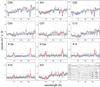 |
Fig. 1. X-ray grating spectra of NGC 5548 in the 16−20 Å band. All spectra are shown in the observed frame. The best-fit baseline models (described in Sect. 2.2) are shown in red. The baseline models excluding the emission pion components are plotted in blue. The thin green curves show the instrumental effective areas in arbitrary units. The corresponding background spectra are displayed in the bottom right panel. All background data are scaled for clarity. The vertical dashed lines mark the central wavelengths of the two possible peaks, 18.35 Å and 18.72 Å, seen in the X21 spectra (see Sect. 2.5 for details). |
To constrain the possible excess feature better, we stacked the fit residuals of the XMM-Newton RGS and Chandra LETGS data. Following the method of Gu et al. (2018), individual residuals were combined with a weighting based on the counts in each energy bin. As shown in Fig. 2, several features can be identified in the stacked spectra. Both the LETGS and RGS residuals show clear peaks at ∼18.4 Å (restframe 18.1 Å), and the RGS residual might have additional peaks at 22.3 Å, 23.1 Å, and 25.6 Å which might coincide with the O VII Heα triplet, O VI absorption line, and C VI radiative recombination continuum. There are also potential dips in the residuals at the Ne IX Heα triplet (∼13.6 Å) with the LETGS data and O VII radiative recombination continuum (∼ 17.0 Å) with the RGS data. Furthermore, by dividing the full RGS sample into two groups, X01 + X21 and the others, we see in Fig. 2 that the ∼18.4 Å excess mostly comes from X01 + X21, while the other possible peaks and the dip seen in the full residual might originate from the other RGS data. Multiple observations equally contribute to the stacked LETGS residual at 18.4 Å, instead of being dominated by a particular piece of data. The possible temporal property of the excess is discussed in Sect. 2.5.
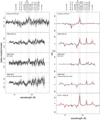 |
Fig. 2. Stacked residuals with respect to the baseline fit (left), and the Gaussian line scan performed on the data (right). In the panel on the right, the results for two different line widths σ = 1000 km s−1 and 4000 km s−1 are shown in black and red, respectively. Notable transitions relevant for the potential features in the stacked residuals are marked with vertical dashed lines. The wavelengths of the transitions are set to the AGN restframe. |
The 18.4 Å wavelength is not consistent with any strong emission or absorption lines in the baseline model. Indeed there are several known nearby atomic transitions that might be relevant, including O VI, O VII, and Fe XVIII lines (Fig. 2). The O VI and O VII transitions are addressed later in Sects. 2.4 and 3.2. The Fe XVIII 2s 2p6 − 2s2 2p4 3p line is unlikely to be responsible for the excess emission since the same ion should also give transitions at 14.44 Å and 16.34 Å in the observed frame. The latter lines have much larger intensities than the former one for both collisional and photoionized plasmas, but they are not seen in the data.
Following the method of Hitomi Collaboration (2018), we calculated the significance of the features by scanning the spectra with a Gaussian line. The Gaussian component has a central wavelength changing from 5 Å to 30 Å, and a width σ set to two trial values, 1000 km s−1 and 4000 km s−1. At each grid wavelength, we refit the spectra with a baseline plus the Gaussian model, and we calculated the ΔC-stat improvement which was then multiplied by the sign of the best-fit normalization to distinguish emission and absorption features. As shown in Fig. 2, the 18.4 Å excess is seen in the Gaussian line scan consistently for the stacked LETGS and the RGS data. The maximal ΔC-stat improvements are 57 and 71 for the two kinds of line widths considered. This improvement comes from both instruments; the ΔC-stat values with the σ = 1000 km s−1 scan are 35 and 45 for the stacked RGS and LETGS data, respectively.
The confidence level of the excess can be determined by taking into account the large number of trials performed to find the line across the wavelength range (the so-called look-elsewhere effect). This effect is addressed in the appendix using both analytic and numerical approaches. Both results show that the putative 18.4 Å feature can be detected above the confidence level of 5σ after the look-elsewhere effect is accounted for. It is the only significant feature detected in both RGS and LETGS bands.
2.4. Systematic effects
Here we investigate the LETGS and RGS spectra further to prove that the detected feature is not an instrumental artifact, a plasma code defect, or a known astrophysical effect. First we examine the effective area curves and instrumental background. As shown in Fig. 1, there are small variations, in particular for the RGS effective area at a 2 − 5% level, some of which are close to the position of the detected line feature. If these variations are not fully calibrated, they might induce artificial spectral features. However, the distributions of the variations are inconsistent with the excess at 18.4 Å, and their amplitudes appear to be much weaker than the excess feature (∼10 − 20%, Fig. 2); therefore, they cannot fully explain the detection. It is even more unlikely for the line detected with the LETGS data to be a false feature in the effective area curves, which are fairly smooth in the wavelength range of interest. Similarly, the line feature cannot be due to known variations in the instrumental background spectra shown in Fig. 1 because these variations are more than one order of magnitude weaker than the observed line intensity at 18.4 Å. Furthermore, we do not see any other bright X-ray source in the RGS extraction regions that might potentially contaminate the observed spectra of the central object.
To further address the instrumental effect, we fit the source spectra obtained in positive and negative orders of the LETGS separately, as well as with the RGS 1 and RGS 2 instruments. It can be seen from Fig. 3 that the stacked fit residuals with positive and negative LETGS orders overlap within their statistical uncertainties. Both data show an excess between 18 Å and 19 Å. Similarly, the residuals with RGS 1 and RGS 2 both have an excess that peaks at 18.4 Å. In addition to that, we also show the residuals obtained with the second-order RGS spectra in Fig. 3. A similar excess can be seen from the second order data, but it is too noisy to provide useful constraints. The consistency between different orders and instruments of the grating data indicates that this excess line feature is unlikely to be an instrumental artifact.
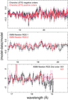 |
Fig. 3. Comparison of the stacked fit residuals with the positive and negative orders of the LETGS (upper panel), as well as the RGS 1 and RGS 2 instruments (middle). The residuals from the RGS second order data of the X01 and X21 observations are shown in the lower panel. |
One remaining possibility is that the feature is a false detection caused by an error in the spectral modeling, for instance a missing transition in the plasma code at 18.4 Å. Such a possibility might be examined by running the calculation with different plasma codes (Hitomi Collaboration 2018), and by fixing possible flaws in the present atomic database (Gu et al. 2019). First we modeled the X21 spectrum using the XSTAR code. The SED of the ionizing source was set to be the same as in Sect. 2.2. The photoionization calculation was run with the semi-analytic warmabs model version 2.41 which is based on the standard population files precalculated with XSTAR v2.58. The absorption and the emission pion components in the baseline were replaced by the absorbing warmabs and photemis models, respectively, while the other components were kept the same. The fit parameters of the XSTAR components are log ξ, NH, and velocity shift. As shown in Fig. 4, there is no significant transition at 18.4 Å with the best-fit XSTAR model, and the excess feature obtained with the SPEX and XSTAR models appears to be similar.
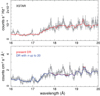 |
Fig. 4. X21 spectrum and the corresponding fit with the XSTAR code (upper panel), and the baseline fit using SPEX with (blue) and without (red) highly excited n > 5 dielectronic recombination transitions (lower). |
We further tested the spectral model by utilizing a more sophisticated atomic data calculation. The emission lines of H-like and He-like ions (in particular oxygen) were calculated up to high principal quantum number n in SPEX, and none of them fall on 18.4 Å (Fig. 2). The Li-like satellite lines, which often show a more complex pattern, are more plausible candidates of the excess emission. Several O VI dielectronic recombination (DR) transitions indeed occur in the range from 18.3 − 18.7 Å. These DR lines were calculated based on a radiative cascade from doubly excited levels, while in the present atomic database we included doubly excited levels only up to n = 5 for O VI. To address the effect of the DR lines from higher shells, we put forward a new calculation of O VI covering singly and doubly excited levels up to n = 20. The level energies, transition probabilities, and radiative branching ratios were obtained using the same approach as described in Gu et al. (2019). We ran the X21 fit again after implementing the new O VI calculation in SPEX. As shown in Fig. 4, the fit with new atomic data is nearly identical to the original one, indicating that the missing DR lines from high-n levels in the photoionization model fall well below the level of the observed excess.
To quantify the excess over the known DR intensity, we allowed the DR line emissivity free to fit. The most relevant transition is 1s2 2s − 1s 2s 6p at a restframe wavelength of 18.06 Å. It can fully account for the observed excess in the X21 spectrum when the intensity of the transition increases by a factor of 62. This factor far exceeds the typical errors in atomic data of the DR lines (Gu et al. 2020), as well as the possible line enhancement due to the external electric field observed in ground-based laboratory (Böhm et al. 2003). Furthermore, it would be rather unexpected that this line would be significantly underestimated, while its neighbor DR lines of similar origin are not, for a photoionized emission source.
Another possible interpretation is a known astrophysical feature which is relevant to either a relativistic broad line, or a dust absorption component. As reported in Branduardi-Raymont et al. (2001), the RGS spectra of MCG-6-30-15 and Mrk 766 show significant excess emission between 18 Å and 19 Å above a nonrelativistic warm absorber model. The observed spectra are better reproduced by relativistically broadened and skewed Lyα lines of O VIII, N VII, and C VI, originating from a combination of gravitational redshift around the black holes and the relativistic beaming due to gas swirling at extreme velocities. We examined this possibility on the NGC 5548 X21 spectrum by adding an O VIII Lyα line at a restframe of 18.96 Å broadened with a relativistic laor profile (Laor 1991) to the baseline model. The new best-fit model is plotted in Fig. 5. We find that the additional relativistic line component does not match with the observed excess at 18.4 Å which is apparently narrower than the laor profile. Thus, the relativistic effect predicted from the standard model is unlikely the source of the feature. One potential caveat here is that the relativistic broadening profile obtained above could be a bit different from those derived by more sophisticated relativistic reflection models such as relxill (García et al. 2014; Dauser et al. 2022), which calculate the angular dependence of the intrinsic reflection emission more accurately.
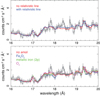 |
Fig. 5. X21 spectrum and the fit with the baseline model broadened with a relativistic laor profile (upper panel), and the fit with the baseline plus an amol component (lower). Results with different compositions of the compound are plotted in blue, green, and magenta. |
An alternative scenario for the excess features observed in the grating spectra of MCG-6-30-15 is the so-called dusty warm absorbers (Lee 2010). It has been proposed that the excess features can be explained by the superposition of O VII absorption lines with the L-shell absorption complex of Fe I, which is likely caused by the dust potentially embedded in the partially ionized outflows (Lee et al. 2001). To test this possibility for NGC 5548, we utilized an amol component in SPEX to model the absorption from the possible dusty or molecular matter around the warm absorbers. The most relevant amol compound is Fe2O3, which contains both O K- and Fe L- edges. At the same time, we also tested the cases with molecular O, as well as with metallic Fe components. As shown in Fig. 5, the dusty components do induce several broad features in the 16−20 Å range; however, they do not reproduce the relatively narrow feature at 18.4 Å. Therefore, the present dust depleted outflow model does not explain the line.
In summary, we report a discovery of a weak emission feature at 18.4 Å using the stacked grating spectrum of NGC 5548. The restframe wavelength is 18.1 Å. The line is seen at a > 5σ significance, accounting for the look-elsewhere effect. We find that it is unlikely an instrumental feature, or a defect in the plasma model. Common astrophysical effects, including a relativistic broad line and a dust absorption component, cannot reproduce the observed excess.
2.5. Line profile and variability
The stacked grating spectra shown in Fig. 2 illustrate an excess that appears to be broader than a single narrow line feature. As described in Sect. 2.3, several observations (Fig. 1) further imply that the excess feature might contain two emission peaks, one centered at around 18.1 − 18.5 Å and the other at 18.4 − 18.8 Å. The best example, X21, clearly shows a double-peaked line profile at 18.35 Å and 18.72 Å. For all the observations, except for C05, the second peak at a longer wavelength appears to be dimmer than the first one. To sufficiently model the observed excess, we added two Gaussian components into the baseline model. Their central wavelengths were free to vary within the ranges of 18.1 − 18.5 Å (hereafter G1) and 18.4 − 18.8 Å (hereafter G2), while the line intensities and widths were set free. In several cases, the width of the second Gaussian component could not be constrained, so we fixed it to that of the first one.
This model allows us to assess the possible variation of the excess. First we assume that the Gaussian components remain unabsorbed by the outflowing components (i.e., X-ray obscurers and warm absorbers), while corrected only for the cosmological redshift and Galactic absorption using the hot component. The central wavelengths and the normalizations of the Gaussian components can be constrained for each observation. We plot in Fig. 6 the central wavelength variation of the G1 component as a function of the hardness ratio (H − S)/(H + S) derived from the best-fit baseline model, where H is the hard X-ray flux in the 1.5 − 10.0 keV band and S is the soft flux in 0.3 − 1.5 keV. A large hardness ratio is often seen when strong X-ray obscuration occurs in this source (Mehdipour et al. 2015, 2017, 2022; Kaastra et al. 2018). We do not plot the wavelength of the G2 component as it is poorly constrained in several observations. It can be seen that the central wavelength of the G1 component does not vary significantly over the past 20 years, while the hardness ratio changes significantly between −0.3 and 0.5. Figure 6b plots the combined normalization of the two Gaussian components as a function of the hardness ratio. The line intensity appears to decrease as the hardness ratio increases. Fitting the normalization-hardness ratio diagram with a constant horizontal line yields a reduced χ2 of 10.05, indicating a probability p value of 0.0015. This means that the intensity of the observed excess, if unabsorbed by the AGN absorbers, significantly varies in the past observations.
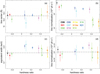 |
Fig. 6. Variation of the observed excess feature as a function of the average hardness ratio (H − S)/(H + S) (see Sect. 2.5). Panels a–d: variations of the central wavelength of the G1 component described in Sect. 2.5, the total G1 + G2 normalization assuming unabsorbed Gaussian components, the total equivalent width, and total normalization assuming absorption. The vertical lines in (a), (b), and (d) show the fits with a constant model. |
Interestingly, as shown in Fig. 6c, the combined equivalent width of the two Gaussian components appears to be much less variable than the normalizations of the lines. This is because the obscuration plays an essential role in the continuum and the hardness ratio variation. As the obscuration increased around 2013 (Kaastra et al. 2014), the continuum around 18.4 Å decreased, which cancels out the decreasing intensity of the observed excess around that time, leading to a nearly time-constant equivalent width. This motivates us to address the second possibility that the excess component, represented by the two Gaussian lines, has been affected by the absorbing materials around the AGN, including the obscurers and the warm absorbers. As shown in Fig. 6d, the combined line intensity from this modified model becomes nearly constant, which differs dramatically from Fig. 6b where the line intensity occurs to be strongly variable as a function of the hardness ratio. Therefore, the observed excess could in fact be a constant component if its emission is partially obscured by the outflowing clouds found at ∼0.01 to several parsec from the central engine (Kaastra et al. 2014).
3. Discussion
By examining the stacked XMM-Newton RGS and Chandra LETGS spectra of the archetypal Seyfert 1 galaxy NGC 5548, we detected a weak emission feature around 18.4 Å which consists of one or two peaks above the model. There is no likely candidate for an atomic transition in a photoionized or collisional plasma, except for several very weak satellite transitions from n ≥ 4 of O VI. It is also unlikely to be caused by residuals due to absorption features from matter in gas or dust forms. This signal appears to be relatively bright in the years 1999−2013 and 2021, but rather dim from 2013 to 2016 when the strong obscuration by outflows occurred in this source (Kaastra et al. 2014; Mehdipour et al. 2015). It is unclear whether this possible variation is intrinsic to the source, or if it is caused by the attenuation from the X-ray obscuration and absorption near the center.
A firm interpretation of the observed excess is hindered by the fact that it is merely one or two weak lines. Below we discuss two candidate scenarios, one with a shifted emission line and the other incorporating a different plasma process.
3.1. Blueshifted O VIII line
Blustin & Fabian (2009) reported possible broad excess features found with the XMM-Newton RGS spectrum of the Seyfert 1 galaxy 1H0707−495. In their Fig. 2, a broad emission feature is seen at a restframe of 18.6 Å, which has been interpreted as a blueshifted component of an O VIII line. Deeper XMM-Newton data of 1H0707−495 reveal that the emitting gas has a radial velocity of about 8000 km s−1 and a velocity dispersion of 3000 − 6000 km s−1 (Kosec et al. 2018a; Xu et al. 2021). Similar blueshifted emission features are found at the wavelengths of N VII, Fe XVII, Ne X, S XVI, and Fe XXV/Fe XXVI. These lines are interpreted as photoionized emission from a wind component powered by the radiation pressure due to the high accretion rate of the AGN.
Assuming that the NGC 5548 feature is a shifted component of the O VIII Lyα line, the average Doppler velocity is obtained to be 14900 ± 600 km s−1 and the average Gaussian broadening is 800 ± 200 km s−1. The average speed is much higher, while the random motion is milder than those of the blueshifted emission component in 1H0707−495. The excess emission in NGC 5548 would originate from a significantly ionized (e.g., log ξ ≥2) component since no blueshifted O VII counterpart can be detected in the stacked spectrum. As shown in Fig. 7, the observed excess in the X21 spectrum seems to be consistent with a blueshifted log ξ = 2 pion emission component which is added to the baseline model. The new component does not predict any detectable features from other elements elsewhere in the spectrum, including the soft X-ray and Fe K-shell bands. We do not see any evidence for other possible relativistic emission or an absorption line in the Chandra LETGS and the XMM-Newton RGS as well as the EPIC spectra. It is therefore not feasible to constrain the ionization state of the possible emitter with the present data further. It should be noted that the radial Doppler velocity obtained above is clearly higher than those of the known warm absorbers in X-ray (Kaastra et al. 2014; Mehdipour et al. 2015; Di Gesu et al. 2015; Ebrero et al. 2016) as well as the kinematic structures seen at longer wavelengths (Crenshaw et al. 2003; Shapovalova et al. 2004; Arav et al. 2015; Li et al. 2016). It is in better agreement with those of the ultrafast outflows (e.g., Tombesi et al. 2013; Parker et al. 2018), although the ultrafast outflows are often observed as blueshifted absorption lines rather than an emission feature.
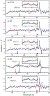 |
Fig. 7. NGC 5548 spectra fit with the baseline plus an additional component. The X21 data and the best-fit blueshifted pion model with log(ξ) = 2 (Sect. 3.1) are shown in (a). Panels b and c: plot the X21 spectrum fit with the blueshifted single charge exchange of ionization temperature equal to 0.05 keV, and two charge exchange components of the same temperature. The C13 data with a single charge exchange component is shown in (d). The X21 spectrum with a redshifted charge exchange component (an ionization temperature equal to 0.1 keV) is displayed in (e). In all panels, the baseline model is plotted in red, and the baseline plus additional component is shown in blue. The relevant lines of the additional components (pion and cx) are also plotted below the data. The wavelengths of the transitions are given at the AGN restframe, and the intensities are scaled for clarity. For better comparison, the spectra and the models around the 18.4 Å feature are also shown in the insets. |
3.2. Charge exchange model
Another potential scenario is that the detected excess comes from an extra plasma component. Here we address the possibility of a charge exchange line (Gu et al. 2015, 2016, 2017, 2018). The charge exchange emission originates from the capture of a single electron from the target neutral hydrogen atom to a highly charged projectile ion that collides with the neutral target,
 (1)
(1)
where Xq+ is the highly charged ion, nl denotes the principal quantum number and orbital angular momentum of the captured electron, 2S + 1L is the total spin S and total orbital angular momentum L, and δE is the kinetic energy released in the collision. The electron is first captured in a highly excited state with a large quantum number n, then it relaxes via a cascade.
As pointed out in Sect. 2.4, the best matching atomic transitions of the observed feature are the Li-like oxygen satellite lines from states with one core excitation electron (1s − 2s), and the other electron at a shell with a large principal quantum number n. Although most existing charge exchange calculations do not consider core excitation (e.g., Smith et al. 2012, 2014; Gu et al. 2016; Cumbee et al. 2018), this process does occur, and the core excitation with charge exchange has already been observed in laboratory for the Li-like line production (e.g., Pepmiller et al. 1983; Tanis et al. 1985; Lee et al. 1991 and references therein). Although oxygen was not tested in their experiments, it is natural to expect that core excitation occurs to Li-like oxygen production. The core excitation process in charge of exchange is often referred to as transfer excitation, which occurs simultaneously with the electron capture, forming doubly excited intermediate states. The excitation can be mediated either by the Coulomb field interaction of the target proton, or through the resonant ion-electron interaction analogously to dielectronic recombination. Laboratory measurements on a Ne6+ + He collision (Beijers et al. 1992) suggested that the charge exchange cross section with core excitation can be comparable with those for the conventional core-conserving capture at low collision velocities. Other measurements further demonstrated that the captured electron primarily falls onto high-n orbits in both core excitation and core-conserving cases (e.g., Raphaelian et al. 1991; Tanis et al. 1985). Therefore, we consider the charge exchange with core excitation as a plausible candidate producing the doubly excited high-n Li-like O lines.
Because the charge exchange with core excitation is not available in the present SPEX cx model (Gu et al. 2016), we built a simple model on O6+ (O VII) + H to test our scenario. This process would end up with a proton and a O5+ (O VI) ion in an excited state. First we assumed that the total cross section with core excitation is the same as the present core-conserving process that is available in SPEX. Then we let the core electron excite via 1s − 2s and 1s − 2p channels, and we applied the present velocity-dependent n and l distributions, obtained in the theoretical calculation using the quantum molecular-orbital close-coupling method (Wu et al. 2012), to the level-resolved cross sections of the captured electron. The new calculations were inserted in the SPEX atomic database, making it possible to evaluate the spectrum of O6+ + H, taking both the core-exciting and core-conserving processes into account. As the O6+ (O VII) has the strongest emission lines in the observed spectra, it is feasible to expect that this ion is responsible for the most relevant charge exchange feature.
This simple model predicts that the core-conserving charge exchange of O6+ + H produces O VI emission lines (e.g., 2s − 4p and 2s − 5p) mostly at a restframe ∼110 Å, while the core-exciting capture gives several transitions including, in particular, the 1s2 2s − 1s 2s 4p (18.35 Å and 18.57 Å) and 1s2 2s − 1s 2s 2p (22.36 Å), which might be relevant to the observed excess in NGC 5548. By refitting the X21 spectrum with the baseline plus the new cx model, we find that the primary excess feature at 18.4 Å is consistent with the 1s2 2s − 1s 2s 4p line blueshifted by a Doppler velocity of 7500 ± 500 km s−1. The best-fit ionization temperature is 0.05 ± 0.02 keV, and the velocity dispersion of the charge exchange component was measured to be ≤1050 km s−1. Adding the new charge exchange component improves the C-statistics by 51 for an expected value of 1893, with a probability of 7 × 10⁻⁹ that the better fit is caused by chance. As shown in Fig. 7, besides the O VI lines, the new component introduces a few C V lines, including, in particular, 1s2 − 1s 2s, 1s2 − 1s 2p, and 1s2 − 1s 3p at restframe 41.47 Å, 40.27 Å, and 34.97 Å, respectively. These C V lines are consistent with the LETGS data, although the ΔC-stat is not enough for a significant detection. Any other charge exchange lines in the soft X-ray and the UV ranges are expected to be weaker by at least 50 than the O VI 1s2 2s − 1s 2s 4p line, and they are unlikely to be visible with the existing observations using Chandra, XMM-Newton, and Hubble.
It is possible that these charge exchange lines come from the mixing of a warm outflow, partially ionized by either a photon or collision, with an adjacent cold layer that is not yet ionized. The cold matter could be a part of the outflow itself, or it may belong to a component in the close environment, for example the dusty torus. The outflow velocity of the possible O6+ gas is slightly larger than that of the X-ray obscurer, ≤5000 km s−1, measured from the associated broad UV absorption lines in the Hubble cosmic origins spectrograph data (Kaastra et al. 2014). It could be compared with the velocity dispersions of the broad UV (up to ∼6800 km s−1, Kaastra et al. 2014) and X-ray (7400 km s−1, Mao et al. 2018) emission. These agreements suggest that the observed emission feature might originate from the central region of the AGN. However, it must be noted that the current estimations of the radial velocity as well as the line intensities using the charge exchange model fully rely on the nl distribution of core-exciting O6+ + H capture, which is obtained based on a crude assumption. The line wavelengths and intensities should further vary as a function of the O6+ + H collision velocity that is still very uncertain. Any further implication on the origin of the possible emission would be too speculative before the present charge exchange modeling is verified with an ab initio theoretical calculation or a dedicated laboratory measurement.
The possible secondary peak at 18.4 − 18.8 Å (Sect. 2.5), seen in particular in X21 and C05, cannot be accounted for by the same charge exchange component. It might indicate another velocity component within the outflowing cloud. To test this possibility, we refit the X21 spectrum using the baseline plus two charge exchange components. All parameters of the second component, except for the normalization, redshift, and velocity dispersion, were fixed to those of the first one. The possible peak at 18.7 Å can be reproduced by a cx component blueshifted by an outflowing velocity of 2500 ± 900 km s−1, with a line width ≤400 km s−1.
Besides O6+ + H, the core-conserving capture of O7++ H produces emission lines at restframe wavelengths of 17.77 Å (1s2 − 1s 4p) and 17.40 Å (1s2 − 1s 5p), providing another potential candidate for the observed excess. These lines were calculated based on the existing cx model which incorporates the cross section calculated using the quantum molecular-orbital close-coupling method (e.g., Nolte et al. 2012). To fit the observed excess, the 1s2 − 1s 4p and 1s2 − 1s 5p lines need to be redshifted by Doppler velocities of ∼5000 km s−1 and ∼11 000 km s−1 with respect to the AGN. In practice, however, the O7++ H charge exchange would also produce a strong redshifted 1s − 2s forbidden line which was not seen in the observed data (Fig. 7e). The 2s level is mostly populated by cascades from n = 4 and 5 intermediate levels. Reducing the 1s − 2s transition would require a major revision to the l and S distributions of the captured electron, which is rather unlikely given the available results from the laboratory measurements (Mullen et al. 2016; Cumbee et al. 2018). Therefore, the O7++ H charge exchange cannot be the primary process.
4. Conclusion
By reanalyzing all the available XMM-Newton RGS and Chandra LETGS spectra of the Seyfert 1 galaxy NGC 5548, we detected an emission-like feature at 18.4 Å (restframe 18.1 Å). This feature is weak, with an equivalent width ≤10 eV. Despite this, the stacked significance reaches 5σ in taking the look-elsewhere effect into account. The new feature seems to be either intrinsically variable in intensity, or affected by the absorption components that changed over time. We demonstrate that the known systematic issues, including the calibration defects, the missing atomic lines, and the secondary astrophysical effects, cannot significantly affect the detection. The remaining possibilities are the charge exchange emission from the outflowing wind of moderate radial velocity, or a photoionized emission component from the very high speed wind. Disentangling these possibilities is impossible given the present data, and has to wait until the launch of XRISM, Arcus, and Athena.
Acknowledgments
SRON is supported financially by NWO, the Netherlands Organization for Scientific Research. SB acknowledges financial support from ASI under grants ASIINAFI/037/12/0 and no. 2017-14-H.O and from PRIN MIUR project “Black Hole winds and the Baryon Life Cycle of Galaxies: the stoneguest at the galaxy evolution supper”, contract no. 2017PH3WAT. BDM acknowledges support from a Ramón y Cajal Fellowship (RYC2018-025950-I) and the Spanish MINECO grant PID2020-117252GB-I00.
References
- Arav, N., Chamberlain, C., Kriss, G. A., et al. 2015, A&A, 577, A37 [NASA ADS] [CrossRef] [EDP Sciences] [Google Scholar]
- Beijers, J. P. M., Hoekstra, R., Morgenstern, R., & de Heer, F. J. 1992, J. Phys. B At. Mol. Phys., 25, 4851 [NASA ADS] [CrossRef] [Google Scholar]
- Blustin, A. J., & Fabian, A. C. 2009, MNRAS, 399, L169 [NASA ADS] [CrossRef] [Google Scholar]
- Böhm, S., Müller, A., Schippers, S., et al. 2003, A&A, 405, 1157 [NASA ADS] [CrossRef] [EDP Sciences] [Google Scholar]
- Bottorff, M. C., Korista, K. T., & Shlosman, I. 2000, ApJ, 537, 134 [NASA ADS] [CrossRef] [Google Scholar]
- Branduardi-Raymont, G., Sako, M., Kahn, S. M., et al. 2001, A&A, 365, L140 [NASA ADS] [CrossRef] [EDP Sciences] [Google Scholar]
- Cappi, M., De Marco, B., Ponti, G., et al. 2016, A&A, 592, A27 [NASA ADS] [CrossRef] [EDP Sciences] [Google Scholar]
- Costantini, E., Kaastra, J. S., Arav, N., et al. 2007, A&A, 461, 121 [CrossRef] [EDP Sciences] [Google Scholar]
- Crenshaw, D. M., Kraemer, S. B., & George, I. M. 2003, ARA&A, 41, 117 [NASA ADS] [CrossRef] [Google Scholar]
- Cumbee, R. S., Mullen, P. D., Lyons, D., et al. 2018, ApJ, 852, 7 [Google Scholar]
- Dauser, T., García, J. A., Joyce, A., et al. 2022, MNRAS, 514, 3965 [NASA ADS] [CrossRef] [Google Scholar]
- Dehghanian, M., Ferland, G. J., Kriss, G. A., et al. 2019a, ApJ, 877, 119 [NASA ADS] [CrossRef] [Google Scholar]
- Dehghanian, M., Ferland, G. J., Peterson, B. M., et al. 2019b, ApJ, 882, L30 [NASA ADS] [CrossRef] [Google Scholar]
- Detmers, R. G., Kaastra, J. S., & McHardy, I. M. 2009, A&A, 504, 409 [NASA ADS] [CrossRef] [EDP Sciences] [Google Scholar]
- de Vaucouleurs, G., de Vaucouleurs, A., Corwin, Herold G., Jr., et al. 1991, Third Reference Catalogue of Bright Galaxies [Google Scholar]
- Di Gesu, L., Costantini, E., Ebrero, J., et al. 2015, A&A, 579, A42 [NASA ADS] [CrossRef] [EDP Sciences] [Google Scholar]
- Ebrero, J., Kaastra, J. S., Kriss, G. A., et al. 2016, A&A, 587, A129 [NASA ADS] [CrossRef] [EDP Sciences] [Google Scholar]
- García, J., Dauser, T., Lohfink, A., et al. 2014, ApJ, 782, 76 [Google Scholar]
- Giustini, M., Costantini, E., De Marco, B., et al. 2017, A&A, 597, A66 [NASA ADS] [CrossRef] [EDP Sciences] [Google Scholar]
- Goad, M. R., Korista, K. T., De Rosa, G., et al. 2016, ApJ, 824, 11 [NASA ADS] [CrossRef] [Google Scholar]
- Grafton-Waters, S., Branduardi-Raymont, G., Mehdipour, M., et al. 2020, A&A, 633, A62 [EDP Sciences] [Google Scholar]
- Grafton-Waters, S., Branduardi-Raymont, G., Mehdipour, M., et al. 2021, A&A, 649, A162 [NASA ADS] [CrossRef] [EDP Sciences] [Google Scholar]
- Gu, L., Kaastra, J., Raassen, A. J. J., et al. 2015, A&A, 584, L11 [NASA ADS] [CrossRef] [EDP Sciences] [Google Scholar]
- Gu, L., Kaastra, J., & Raassen, A. J. J. 2016, A&A, 588, A52 [NASA ADS] [CrossRef] [EDP Sciences] [Google Scholar]
- Gu, L., Mao, J., O’Dea, C. P., et al. 2017, A&A, 601, A45 [NASA ADS] [CrossRef] [EDP Sciences] [Google Scholar]
- Gu, L., Mao, J., de Plaa, J., et al. 2018, A&A, 611, A26 [NASA ADS] [CrossRef] [EDP Sciences] [Google Scholar]
- Gu, L., Raassen, A. J. J., Mao, J., et al. 2019, A&A, 627, A51 [NASA ADS] [CrossRef] [EDP Sciences] [Google Scholar]
- Gu, L., Shah, C., Mao, J., et al. 2020, A&A, 641, A93 [NASA ADS] [CrossRef] [EDP Sciences] [Google Scholar]
- Guainazzi, M., & Bianchi, S. 2007, MNRAS, 374, 1290 [Google Scholar]
- Hitomi Collaboration (Aharonian, F., et al.) 2018, PASJ, 70, 12 [NASA ADS] [Google Scholar]
- Kaastra, J. S., & Bleeker, J. A. M. 2016, A&A, 587, A151 [NASA ADS] [CrossRef] [EDP Sciences] [Google Scholar]
- Kaastra, J. S., Mewe, R., & Nieuwenhuijzen, H. 1996, in UV and X-ray Spectroscopy of Astrophysical and Laboratory Plasmas, eds. K. Yamashita, & T. Watanabe, 411 [Google Scholar]
- Kaastra, J. S., Mewe, R., Liedahl, D. A., Komossa, S., & Brinkman, A. C. 2000, A&A, 354, L83 [NASA ADS] [Google Scholar]
- Kaastra, J. S., Detmers, R. G., Mehdipour, M., et al. 2012, A&A, 539, A117 [NASA ADS] [CrossRef] [EDP Sciences] [Google Scholar]
- Kaastra, J. S., Kriss, G. A., Cappi, M., et al. 2014, Science, 345, 64 [Google Scholar]
- Kaastra, J. S., Mehdipour, M., Behar, E., et al. 2018, A&A, 619, A112 [NASA ADS] [CrossRef] [EDP Sciences] [Google Scholar]
- Kaastra, J. S., Raassen, A. J. J., de Plaa, J., & Gu, L. 2020, SPEX X-ray Spectral Fitting Package [Google Scholar]
- Kosec, P., Buisson, D. J. K., Parker, M. L., et al. 2018a, MNRAS, 481, 947 [Google Scholar]
- Kosec, P., Pinto, C., Fabian, A. C., & Walton, D. J. 2018b, MNRAS, 473, 5680 [NASA ADS] [CrossRef] [Google Scholar]
- Kriss, G. A., De Rosa, G., Ely, J., et al. 2019, ApJ, 881, 153 [NASA ADS] [CrossRef] [Google Scholar]
- Landt, H., Ward, M. J., Steenbrugge, K. C., & Ferland, G. J. 2015, MNRAS, 454, 3688 [NASA ADS] [CrossRef] [Google Scholar]
- Landt, H., Ward, M. J., Kynoch, D., et al. 2019, MNRAS, 489, 1572 [NASA ADS] [CrossRef] [Google Scholar]
- Laor, A. 1991, ApJ, 376, 90 [Google Scholar]
- Lee, J. C. 2010, Space Sci. Rev., 157, 93 [NASA ADS] [CrossRef] [Google Scholar]
- Lee, D. H., Richard, P., Sanders, J. M., et al. 1991, Phys. Rev. A, 44, 1636 [NASA ADS] [CrossRef] [Google Scholar]
- Lee, J. C., Ogle, P. M., Canizares, C. R., et al. 2001, ApJ, 554, L13 [NASA ADS] [CrossRef] [Google Scholar]
- Li, Y.-R., Wang, J.-M., Ho, L. C., et al. 2016, ApJ, 822, 4 [NASA ADS] [CrossRef] [Google Scholar]
- Longinotti, A. L., Costantini, E., Petrucci, P. O., et al. 2010, A&A, 510, A92 [NASA ADS] [CrossRef] [EDP Sciences] [Google Scholar]
- Mao, J., Kaastra, J. S., Mehdipour, M., et al. 2017, A&A, 607, A100 [NASA ADS] [CrossRef] [EDP Sciences] [Google Scholar]
- Mao, J., Kaastra, J. S., Mehdipour, M., et al. 2018, A&A, 612, A18 [NASA ADS] [CrossRef] [EDP Sciences] [Google Scholar]
- Mao, J., Mehdipour, M., Kaastra, J. S., et al. 2019, A&A, 621, A99 [NASA ADS] [CrossRef] [EDP Sciences] [Google Scholar]
- McKernan, B., Yaqoob, T., & Reynolds, C. S. 2007, MNRAS, 379, 1359 [NASA ADS] [CrossRef] [Google Scholar]
- Mehdipour, M., Kaastra, J. S., Kriss, G. A., et al. 2015, A&A, 575, A22 [NASA ADS] [CrossRef] [EDP Sciences] [Google Scholar]
- Mehdipour, M., Kaastra, J. S., Kriss, G. A., et al. 2017, A&A, 607, A28 [NASA ADS] [CrossRef] [EDP Sciences] [Google Scholar]
- Mehdipour, M., Kriss, G. A., Brenneman, L. W., et al. 2022, ApJ, 925, 84 [NASA ADS] [CrossRef] [Google Scholar]
- Mullen, P. D., Cumbee, R. S., Lyons, D., & Stancil, P. C. 2016, ApJS, 224, 31 [NASA ADS] [CrossRef] [Google Scholar]
- Nolte, J. L., Stancil, P. C., Liebermann, H. P., et al. 2012, J. Phys. B At. Mol. Phys., 45, 245202 [NASA ADS] [CrossRef] [Google Scholar]
- Parker, M. L., Pinto, C., Fabian, A. C., et al. 2017, Nature, 543, 83 [Google Scholar]
- Parker, M. L., Buisson, D. J. K., Jiang, J., et al. 2018, MNRAS, 479, L45 [NASA ADS] [Google Scholar]
- Pepmiller, P. L., Richard, P., Newcomb, J., et al. 1983, IEEE Trans. Nucl. Sci., 30, 1002 [CrossRef] [Google Scholar]
- Pinto, C., Alston, W., Parker, M. L., et al. 2018, MNRAS, 476, 1021 [NASA ADS] [CrossRef] [Google Scholar]
- Pinto, C., Walton, D. J., Kara, E., et al. 2020, MNRAS, 492, 4646 [Google Scholar]
- Pinto, C., Soria, R., Walton, D. J., et al. 2021, MNRAS, 505, 5058 [NASA ADS] [CrossRef] [Google Scholar]
- Pounds, K. A., Nixon, C. J., Lobban, A., & King, A. R. 2018, MNRAS, 481, 1832 [NASA ADS] [Google Scholar]
- Raphaelian, M. L. A., Berry, H. G., Berrah Mansour, N., & Schneider, D. 1991, Phys. Rev. A, 43, 4071 [NASA ADS] [CrossRef] [Google Scholar]
- Reeves, J. N., Braito, V., Chartas, G., et al. 2020, ApJ, 895, 37 [Google Scholar]
- Reynolds, C. S. 2016, Astron. Nachr., 337, 404 [NASA ADS] [CrossRef] [Google Scholar]
- Shapovalova, A. I., Doroshenko, V. T., Bochkarev, N. G., et al. 2004, A&A, 422, 925 [NASA ADS] [CrossRef] [EDP Sciences] [Google Scholar]
- Smith, R. K., Foster, A. R., & Brickhouse, N. S. 2012, Astron. Nachr., 333, 301 [NASA ADS] [CrossRef] [Google Scholar]
- Smith, R. K., Foster, A. R., Edgar, R. J., & Brickhouse, N. S. 2014, ApJ, 787, 77 [NASA ADS] [CrossRef] [Google Scholar]
- Steenbrugge, K. C., Kaastra, J. S., Crenshaw, D. M., et al. 2005, A&A, 434, 569 [NASA ADS] [CrossRef] [EDP Sciences] [Google Scholar]
- Tanis, J. A., Bernstein, E. M., Clark, M. W., et al. 1985, Phys. Rev. A, 31, 4040 [NASA ADS] [CrossRef] [Google Scholar]
- Tombesi, F., Cappi, M., Reeves, J. N., et al. 2010, A&A, 521, A57 [NASA ADS] [CrossRef] [EDP Sciences] [Google Scholar]
- Tombesi, F., Cappi, M., Reeves, J. N., et al. 2013, MNRAS, 430, 1102 [Google Scholar]
- Turner, T. J., & Miller, L. 2009, A&ARv, 17, 47 [Google Scholar]
- Ursini, F., Boissay, R., Petrucci, P. O., et al. 2015, A&A, 577, A38 [NASA ADS] [CrossRef] [EDP Sciences] [Google Scholar]
- Vaughan, S., & Uttley, P. 2008, MNRAS, 390, 421 [NASA ADS] [CrossRef] [Google Scholar]
- Wakker, B. P., Lockman, F. J., & Brown, J. M. 2011, ApJ, 728, 159 [NASA ADS] [CrossRef] [Google Scholar]
- Whewell, M., Branduardi-Raymont, G., Kaastra, J. S., et al. 2015, A&A, 581, A79 [NASA ADS] [CrossRef] [EDP Sciences] [Google Scholar]
- Wildy, C., Landt, H., Ward, M. J., Czerny, B., & Kynoch, D. 2021, MNRAS, 500, 2063 [Google Scholar]
- Wu, Y., Stancil, P. C., Schultz, D. R., et al. 2012, J. Phys. B At. Mol. Phys., 45, 235201 [NASA ADS] [CrossRef] [Google Scholar]
- Xu, Y., Pinto, C., Bianchi, S., et al. 2021, MNRAS, 508, 6049 [NASA ADS] [CrossRef] [Google Scholar]
Appendix A: Significance of the excess
The ΔC-stat reported in § 2.3 cannot be directly used to determine the confidence level of the feature. This is due to the parameter space and wavelength range explored in the Gaussian scan, and the possibility of detecting a random excess feature from the look-elsewhere effect.
First we address this effect in an analytic way. Assuming that the residual data points (Zi, i = [1, n]) follow a normal distribution, we define the probability of an individual data point P(Zi ≤ X) = 1 − Φ(X), where X is the confidence level, and Φ(X) is the likelihood that the null hypothesis is true. To have all Zi ≤ X, the probability becomes P(Zi ≤ X)n ≈ 1 − nΦ(X) for Φ(X)≪1, where n is the number of effective resolving units.
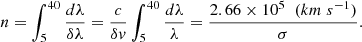
The size of the resolving unit can be obtained as δλ = (δv/c)λ, where δv = 2.35σ is the full width at half maximum of the scanning Gaussian component, and c is the speed of light. The total number of resolving units in the 5 − 40 Å band is
 (A.1)
(A.1)
For the Gaussian σ = 1000 km s−1 and 4000 km s−1, the resolving unit numbers are 266 and 67 per instrument, respectively. These numbers were determined independent of the instruments used. For the observed C-stat improvements ΔC-stat = 57 and 71 (§ 2.3), the null hypothesis probabilities Φ(X) are 2.2 × 10⁻¹⁴ and 1.8 × 10⁻¹⁷ at each individual data point, respectively. The modified probabilities nΦ(X) taking the look-elsewhere effect of the scan into account become 1.2 × 10⁻¹¹ and 2.4 × 10⁻¹⁵. Therefore, the significances of the feature are estimated to be 6.6σ and 7.8σ for the two kinds of Gaussian widths considered.
Besides the analytic approach, it is also possible to quantify the probability of detecting random features using a Monte-Carlo simulation. Following the approach of Kosec et al. (2018b) and Pinto et al. (2020), we simulated 1 × 10⁵ LETGS and RGS spectra based on the baseline model. The LETGS and RGS exposures were set to the real values. The residual of each set of simulated spectra has been scanned using the Gaussian line with σ = 1000 km s−1, and the occurrence of ΔC-stat improvement has been recorded in Figure A.1. The logarithm of the occurrence can be well described by a linear equation with a slope of −0.178 ± 0.007, which allows one to infer a ΔC-stat = 33.3 ± 1.2 for a 4.4σ event with an expected frequency of 1 × 10⁻⁵.
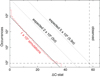 |
Fig. A.1. Histogram of 1 × 10⁵ runs of the Monto Carlo simulation of the NGC 5548 spectrum. The thick black line represents the corresponding power-law fit of the histogram, and the thin black lines show the expected results of 2 × 10⁶ and 5 × 10⁸ simulations. The vertical dashed line marks the observed ΔC-stat = 57 derived with the scan on the observed data using a Gaussian line with σ= 1000 km s−1. |
It is too computationally expensive to calculate the ΔC-stat distribution for 5σ directly which requires a sample of 2 × 10⁶. However, it would be possible to extrapolate from the existing 1 × 10⁵ run. As reported in Pinto et al. (2021), the slope of ΔC-stat distribution obtained with a 2 × 10⁴ simulation on a grating spectrum appears to be in good agreement with those obtained with 2 × 10³ and 5 × 10⁴ simulations. Therefore we predict the ΔC-stat distribution of 2 × 10⁶ simulations using the linear equation with a slope of −0.178. It would suggest a 5σ detection with a ΔC-stat = 45.9 ± 1.6.
As shown in Figure A.1, the above scaling predicts that the observed total ΔC-stat = 57 is consistent with a confidence level of about 5.9σ. This is slightly lower than the significance (6.6σ) obtained in the analytic way. Since the numerical simulations produce more realistic distributions of the spectral residuals, we consider the numerical value (5.9σ) as a better estimate of the confidence level of the putative 18.4 Å feature.
All Tables
All Figures
|
Fig. 1. X-ray grating spectra of NGC 5548 in the 16−20 Å band. All spectra are shown in the observed frame. The best-fit baseline models (described in Sect. 2.2) are shown in red. The baseline models excluding the emission pion components are plotted in blue. The thin green curves show the instrumental effective areas in arbitrary units. The corresponding background spectra are displayed in the bottom right panel. All background data are scaled for clarity. The vertical dashed lines mark the central wavelengths of the two possible peaks, 18.35 Å and 18.72 Å, seen in the X21 spectra (see Sect. 2.5 for details). |
| In the text | |
|
Fig. 2. Stacked residuals with respect to the baseline fit (left), and the Gaussian line scan performed on the data (right). In the panel on the right, the results for two different line widths σ = 1000 km s−1 and 4000 km s−1 are shown in black and red, respectively. Notable transitions relevant for the potential features in the stacked residuals are marked with vertical dashed lines. The wavelengths of the transitions are set to the AGN restframe. |
| In the text | |
|
Fig. 3. Comparison of the stacked fit residuals with the positive and negative orders of the LETGS (upper panel), as well as the RGS 1 and RGS 2 instruments (middle). The residuals from the RGS second order data of the X01 and X21 observations are shown in the lower panel. |
| In the text | |
|
Fig. 4. X21 spectrum and the corresponding fit with the XSTAR code (upper panel), and the baseline fit using SPEX with (blue) and without (red) highly excited n > 5 dielectronic recombination transitions (lower). |
| In the text | |
|
Fig. 5. X21 spectrum and the fit with the baseline model broadened with a relativistic laor profile (upper panel), and the fit with the baseline plus an amol component (lower). Results with different compositions of the compound are plotted in blue, green, and magenta. |
| In the text | |
|
Fig. 6. Variation of the observed excess feature as a function of the average hardness ratio (H − S)/(H + S) (see Sect. 2.5). Panels a–d: variations of the central wavelength of the G1 component described in Sect. 2.5, the total G1 + G2 normalization assuming unabsorbed Gaussian components, the total equivalent width, and total normalization assuming absorption. The vertical lines in (a), (b), and (d) show the fits with a constant model. |
| In the text | |
|
Fig. 7. NGC 5548 spectra fit with the baseline plus an additional component. The X21 data and the best-fit blueshifted pion model with log(ξ) = 2 (Sect. 3.1) are shown in (a). Panels b and c: plot the X21 spectrum fit with the blueshifted single charge exchange of ionization temperature equal to 0.05 keV, and two charge exchange components of the same temperature. The C13 data with a single charge exchange component is shown in (d). The X21 spectrum with a redshifted charge exchange component (an ionization temperature equal to 0.1 keV) is displayed in (e). In all panels, the baseline model is plotted in red, and the baseline plus additional component is shown in blue. The relevant lines of the additional components (pion and cx) are also plotted below the data. The wavelengths of the transitions are given at the AGN restframe, and the intensities are scaled for clarity. For better comparison, the spectra and the models around the 18.4 Å feature are also shown in the insets. |
| In the text | |
|
Fig. A.1. Histogram of 1 × 10⁵ runs of the Monto Carlo simulation of the NGC 5548 spectrum. The thick black line represents the corresponding power-law fit of the histogram, and the thin black lines show the expected results of 2 × 10⁶ and 5 × 10⁸ simulations. The vertical dashed line marks the observed ΔC-stat = 57 derived with the scan on the observed data using a Gaussian line with σ= 1000 km s−1. |
| In the text | |
Current usage metrics show cumulative count of Article Views (full-text article views including HTML views, PDF and ePub downloads, according to the available data) and Abstracts Views on Vision4Press platform.
Data correspond to usage on the plateform after 2015. The current usage metrics is available 48-96 hours after online publication and is updated daily on week days.
Initial download of the metrics may take a while.