| Issue |
A&A
Volume 664, August 2022
|
|
|---|---|---|
| Article Number | A42 | |
| Number of page(s) | 20 | |
| Section | Numerical methods and codes | |
| DOI | https://doi.org/10.1051/0004-6361/202243712 | |
| Published online | 05 August 2022 | |
The halo-finding problem revisited: a deep revision of the ASOHF code
1
Departament d’Astronomia i Astrofísica, Universitat de València,
46100
Burjassot (València),
Spain
e-mail: This email address is being protected from spambots. You need JavaScript enabled to view it.
2
Observatori Astronòmic, Universitat de València,
46980
Paterna (València),
Spain
Received:
5
April
2022
Accepted:
4
May
2022
Abstract
Context. New-generation cosmological simulations are providing huge amounts of data, whose analysis becomes itself a pressing computational problem. In particular, the identification of gravitationally bound structures, known as halo finding, is one of the main analyses. Several codes that were developed for this task have been presented during the past years.
Aims. We present a deep revision of the code ASOHF. The algorithm was thoroughly redesigned in order to improve its capabilities of finding bound structures and substructures using both dark matter particles and stars, its parallel performance, and its abilities of handling simulation outputs with vast amounts of particles. This upgraded version of ASOHF is conceived to be a publicly available tool.
Methods. A battery of idealised and realistic tests are presented in order to assess the performance of the new version of the halo finder.
Results. In the idealised tests, ASOHF produces excellent results. It is able to find virtually all the structures and substructures that we placed within the computational domain. When the code is applied to realistic data from simulations, the performance of our finder is fully consistent with the results from other commonly used halo finders. The performance in substructure detection is remarkable. In addition, ASOHF is extremely efficient in terms of computational cost.
Conclusions. We present a publicly available deeply revised version of the ASOHF halo finder. The new version of the code produces remarkable results in terms of halo and subhalo finding capabilities, parallel performance, and low computational cost.
Key words: large-scale structure of Universe / dark matter / galaxies: clusters: general / galaxies: halos / methods: numerical
© D. Vallés-Pérez et al. 2022
 Open Access article, published by EDP Sciences, under the terms of the Creative Commons Attribution License (https://creativecommons.org/licenses/by/4.0), which permits unrestricted use, distribution, and reproduction in any medium, provided the original work is properly cited.
This article is published in open access under the Subscribe-to-Open model. This email address is being protected from spambots. You need JavaScript enabled to view it. to support open access publication.
1 Introduction
Over the past four decades, numerical simulations of cosmic structure formation have grown significantly in size, dynamical range, and accuracy of the physical model ingredients (see e.g. Vogelsberger et al. 2020; Angulo & Hahn 2022, for recent reviews). In addition to a precise description of the evolution of the dark matter (DM) component of the Universe, current cos-mological simulations have also improved their modelling of the complex baryonic physical processes that shape the properties of the gaseous and the stellar components (see e.g. Planelles et al. 2015, for a review). On the other hand, the outstanding development of computing facilities has led to an increasing computational power and to important advances in algorithms and techniques. This progress has allowed current cosmological simulations to reach a significant level of mass and force resolution, complexity, and realism.
The excellent predictive power of these simulations makes them essential tools in cosmology and astrophysics: they are crucial not only for testing the accepted cosmological paradigm, but for interpreting and analysing how different physical processes inherent to the cosmic evolution affect the observational properties of the Universe we inhabit. To properly exploit the unprecedented capabilities of current advanced cosmological simulations, equivalently complex and sophisticated structure finding algorithms are also required. A proper identification and characterisation of the population of DM haloes and subhaloes, including their abundances, shapes and structure, physical properties, and merging histories, is decisive for understanding the formation and evolution of cosmic structures.
Even when a DM halo is simply a locally overdense gravita-tionally bound structure embedded within the global background density field, the definition of its boundary and, hence, its mass is unavoidably arbitrary. The situation is even more accentuated in the case of subhaloes that are located within larger-scale over-densities, called hosts. In an attempt to overcome these issues, a significant number of halo-finding methods and techniques have been developed in the past decades (e.g. FoF1, Davis et al. 1985; SO2, Cole & Lacey 1996; HOP, Eisenstein & Hut 1998; BDM3, Klypin et al. 1999; Subfind, Springel et al. 2001; Dolag et al. 2009; AHF4, Gill et al. 2004; Knollmann & Knebe 2009; ASOHF5, Planelles & Quilis 2010; Velociraptor, Elahi et al. 2011, 2019; HBT6, Han et al. 2012, 2018; Rockstar, Behroozi et al. 2013; to cite a few).
In general, however, all these algorithms can be broadly divided into three main families of codes: those based on the SO method (Press & Schechter 1974; Cole & Lacey 1996), those relying on the FoF algorithm in 3D configuration space (Davis et al. 1985), and those based on the 6D phase-space FoF (e.g. Diemand et al. 2006). Algorithms in the first class involve locating peaks in the density field and finding the extent of the halo, either by growing spheres until either the enclosed density falls below a given threshold or other properties are met. On the other hand, codes in the second and third categories link particles that are close to each other, either in configuration or in phase-space. Knebe et al. (2011, 2013) reported an exhaustive review and comparison of some of these halo finders. These studies showed that while all codes are able to identify the location of mock isolated haloes and some of their properties (e.g. the maximum circular velocity, υmax), important differences arose for small-scale haloes, especially substructures (Onions et al. 2012, 2013; Hoffmann et al. 2014), or when some properties such as spin and shape were determined.
In addition to DM structures, modern simulations also track the formation of stellar particles from cold gas. These particles cluster and form stellar haloes, or galaxies. While the formation of galaxies is tightly linked to their underlying DM haloes, their different evolutionary histories, properties, and dynamics imply that they deserve to be studied as objects in their own right. Consistently, specific algorithms for these tasks have recently been developed (e.g. Navarro-González et al. 2013; Cañas et al. 2019).
Planelles & Quilis (2010) presented ASOHF, a halo finder based on the SO approach. Although ASOHF was especially designed to be applied to the outcomes of grid-based cosmo-logical simulations, it was adapted to work as a stand-alone halo finder on particle-based simulations. The performance of ASOHF in different scenarios was demonstrated in Knebe et al. (2011). In addition, the code has been employed in a number of works (Planelles & Quilis 2013; Quilis et al. 2017; Martin-Alvarez et al. 2017; Planelles et al. 2018; Vallés-Pérez et al. 2020, 2021). The incessant improvements of cosmological simulations, aided by the ever-growing available computing power, have enormously increased the number of particles and, consequently, the richness of small-scale structures. This demanded a revisit of the process of halo-finding in ASOHF to ensure that small structures are well captured and their properties can be recovered in an unbiased way, and also to guarantee that the code is able to tackle these amounts of data within reasonable computational times.
In this paper we present an upgraded, faster, and more memory-efficient version of ASOHF that is capable of efficiently dealing with the new generation of cosmological simulations that include huge numbers of DM particles, haloes, and substructures. Amongst the main improvements, we present a smoother density interpolation that lowers the computational cost by decreasing the number of spurious density peaks, the addition of complementary unbinding procedures, a new scheme for searching for substructures, the ability of identifying and characterising stellar haloes, and a domain decomposition approach that can lower the computational cost and computing time. On the performance side, the code has been profoundly overhauled in terms of parallelisation and memory requirements. It is now able to analyse simulations with hundreds of millions of particles on desktop workstations within a few minutes at most. This version of ASOHF is publicly available.
The paper is organised as follows. In Sect. 2 we describe the main procedure on which our halo finder relies to identify the samples of haloes, subhaloes, and stellar haloes, as well as additional features such as the domain decomposition scheme and the merger tree. The performance and scalability of ASOHF in some idealised but rather complex tests is shown in Sect. 3. Additionally, in Sect. 4 we test the performance of the code against actual simulation data and compare its performance to other well-known halo finders, and we show the capabilities of ASOHF as a stellar halo finder. Finally, in Sect. 5 we discuss and summarise our results. Appendix A further describes one of the unbinding schemes, while in Appendix B we discuss our estimation of the gravitational binding energy and most-bound particle by sampling.
2 Algorithm
While the original algorithm was introduced by Planelles & Quilis (2010), a large number of modifications and upgrades have been undertaken in order to provide a fast, memory-efficient, and flexible code that is able to tackle a new generation of cosmological simulations, with an increase of several orders of magnitude in the number of DM particles, haloes, and rich substructure. Here we describe the main steps of our halo-finding procedure. The implementation of ASOHF for shared-memory platforms (OpenMP), written in Fortran, is publicly available through the GitHub repository of the code7. The following subsections describe the input data (Sect. 2.1), the process of identifying density peaks (Sect. 2.2), the characterisation of haloes using particles (Sect. 2.3), the substructure identification scheme (Sect. 2.4), the characterisation of stellar haloes (Sect. 2.5), and several additional features and tools of the ASOHF package (Sect. 2.6). Table 1 contains a summary of the parameters of the code that can be configured.
2.1 Input Data
Generally, the input data for ASOHF consist of a list of DM particles, containing the three-dimensional positions and velocities, masses, and a unique integer identifier of each of the Npart particles. While ASOHF was originally envisioned to be coupled to the outputs of the cosmological code MASCLET (Quilis 2004; Quilis et al. 2020), it can work as a fully stand-alone halo finder. The reading routine is fully modular and can easily be adapted to suite the input format of the user8.
2.2 Grid Halo Identification
The identification of haloes relies on the analysis of the underlying continuous density field, which is obtained by means of a grid interpolation from the particle distribution. Originally inherited from MASCLET, since its original version, ASOHF uses an Adaptive Mesh Refinement (AMR) hierarchy of grids to compute the density field on different scales. This enables capture of a large dynamical range in masses and radii. In this section we describe the mesh creation procedure (Sect. 2.2.1), which has been optimised to allow the code to handle even hundreds of thousands of refinement patches in large simulations. Next, we present the new density interpolation scheme (Sect. 2.2.2) that mitigates the effect of sampling noise, and the halo-finding process over the grid (Sect. 2.2.3). It is worth noting that to avoid arbitrariness in defining a given structure, the new version of ASOHF does not deal with peaks within haloes at this stage. This is considered in a later step in Sect. 2.4.
2.2.1 Mesh Creation
A coarse grid of size Nx × Ny × Nz covers the whole domain of the input simulation. On top of this base grid, an arbitrary number of mesh refinement levels is generated by placing patches covering the regions with highest particle number density, each level halving the cell size with respect to the previous one. In particular, we flag as refinable any cell hosting more than a minimum number of particles  . The mesh creation routine then examines all the refinable cells, from densest to least dense, and tries to extend the patch in each direction if the fraction of refinable cells amongst the added cells exceeds
  Only patches with a given minimum size
  are accepted; otherwise, the region is not refined. These quantities
  , and
, and  , as well as the number of refinement levels (nℓ), are free parameters that can be tuned to find a balance between memory usage and resolution. Generally, the latter can be fixed so that the peak resolution matches the force resolution of the simulation. We present in Sect. 3.4.1 a test showing how these parameters work with varying particle resolutions.
Summary of the main parameters that can be tuned to run ASOHF.
2.2.2 Density Interpolation
In our experiments, we find that interpolating particles into cells using the standard cloud-in-cell (CIC) or triangular-shaped cloud (TSC) schemes at the resolution of each AMR patch has a detrimental effect for the purpose of density peak finding because it produces a very large number of peaks due to shot noise. While these false peaks would be removed in subsequent steps when halo properties are refined with particles (Sect. 2.3), they produce an overwhelming computational burden and load imbalance between different threads.
To avoid this, we compute the local density field by spreading each particle, using linear or quadratic kernels, in a cubic cloud with the same volume as the particle sampled in the initial conditions. That is to say, if different particles species (in terms of mass) are present, each one is spread into the AMR grids according to their corresponding kernel sizes, that is, the kernel radius Δxkern,i is set by
 (1)
(1)
with L the box size, Mbox the total mass in the box, and mp,i the mass of the particle i. Alternatively, for simulations with equal-mass particles, the kernel size can be chosen to be determined by the local density in the base grid cell occupied by each particle. This procedure naturally produces a smooth density field that is free of spurious noise while still capturing local features such as the density peaks associated with a hierarchy of substructures.
2.2.3 Halo Finding
Haloes are pre-identified as peaks, that is, local maxima, in the density field, from the coarsest to the finest AMR levels. To do this, ASOHF lists all the (non-overlapping) cells at each AMR level that simultaneously fulfil the following two criteria. First, the cell density is higher than the virial density contrast at a given redshift, Δm,vir(z), computed according to the prescription of Bryan & Norman (1998). Incidentally, we also consider cells whose overdensity exceeds Δm,vir(z)/6 because the density interpolation could smooth the peaks in some situations. We verify with the tests in Sect. 3.1 that further lowering this value does not allow to recover any more haloes. Additionally, the cell must correspond to a local maximum of the density field, that is, its density is higher than that of the 33 neighbouring cells.
The algorithm then iterates over them with decreasing over-density. For each cell, the procedure can be summarised as follows. First, check whether the cell is inside a previously identified halo. If it is, skip it; if not, continue (note that we do not search for substructure at this stage). Then, refine the location of the density peak using the information in higher (i.e. finer) AMR levels, if available, and check that the refined position does not overlap with previously identified haloes. Finally, grow spheres of increasing radii until the enclosed overdensity, measured using the density field, falls below Δm,vir.
This produces a first list of isolated haloes (i.e. that are not substructure), with an estimation of their positions, radii, and masses, which will be refined further by using the whole particle list information in the following step. At this step, haloes can overlap, although no halo centre can be placed inside another halo. These peaks are processed within the substructure-finding step (Sect. 2.4).
2.3 Halo Refinement Using Particles
After they are identified, the halo properties are refined using the particle distribution in several steps as described below. We refer to Sect. 3.1 for a test that shows the capabilities of ASOHF to identify and recover the properties of haloes in an unbiased way. While the basic process (collecting particles, unbinding, and determining the virial radius), common to most SO halo finders, was present in the original version, the new version of ASOHF includes many refinements to improve the quality of the recovered catalogues (e.g. recentring of the density peak or additional unbinding procedures), as well as other features to significantly decrease the computational cost and compute certain halo properties.
Recentring of the density peak. Within the scheme described in Sect. 2.2, the density peak location, as identified within the grid, has an uncertainty of the order of the cell size of the finest grid covering the peak. In order to improve this determination, the first step consists of refining the position of the density peak using particles.
To do this, we consider a cube centred on the estimated density peak, with a side length of 2Δxℓ, with Δxℓ the cell size of the finest patch used to locate the density peak within the grid. We compute the density field in this volume using an ad hoc 43 cells grid, and select as the corrected centre the position of the largest local maximum of the density field. The process is iterated while more than 32 particles are found in the cube. Each time, the cube side lenth is halved, and it is centred on the peak of the previous step. The position found by this procedure is not further changed in the process of halo finding.
Selection of particles. In order to alleviate part of the computational burden associated with traversing the whole particle list, only the particles in a sphere with mean density 〈ρ〉 = min(Δvir,m(z), 200) ρB(z), with ρB(z) the background matter density at redshift z, are kept for each halo. Subsequently, this list is sorted by increasing distance to the halo centre.
Additionally, to boost performance by decreasing the number of array accesses and distance calculations, which are an important performance penalty as the number of particles in the simulation increases, particles are sorted according to their x-component before the whole process of halo finding starts. Then, only a small fraction of the particle list is traversed in order to select the halo particle candidates, in a way similar to a tree search algorithm in one dimension. This effect becomes increasingly stronger as the volume being analysed increases.
Unbinding. A common feature of configuration-space halo finders is the necessity of pruning the particles that are dynamically unrelated to the haloes because particles are initially collected using only spatial information. We perform two complementary, consecutive unbinding procedures that we describe below.
Local escape velocity unbinding. First, the Poisson equation is solved in spherical symmetry for the particle distribution (see Appendix A), yielding the gravitational potential ϕ(r). The escape velocity is then estimated as  . Finally, any particle with velocity (relative to the halo centre of mass reference frame) exceeding its local escape velocity should be flagged as unbound and pruned from the halo.
However, because the bulk velocity of the halo can be severely contaminated by the unbound component, we unbind particles in an iterative way by pruning particles with a speed relative to the centre of mass higher than βυesc(r). In successive steps, we take β = 8, 4, and finally β = βfinal = 2. Each time, the gravitational potential generated by bound particles alone is recomputed. The process is iterated with the last value of β until no new particles are removed in an iteration.
We set βfinal = 2 instead of removing all particles whose speed exceeds the local escape value because these marginally unbound particles may become bound at a later step and will not drift away from the cluster immediately (see e.g. the discussion in Knebe et al. 2013).
Velocity space unbinding. The standard deviation of the particle velocities within the halo, συ, with respect to the centre-of-mass velocity, is computed. Particles whose three-dimensional velocity differs by more than βσυ from the centre-of-mass velocity are pruned. Like in the previous scheme, β is lowered progressively, from β = 6 to β = βfinal = 3. In each step, the centre-of-mass velocity is recomputed for bound particles.
We refer to Sect. 3.3 for two specific tests that show the complementarity of these two unbinding schemes.
Determining spherical overdensity boundaries. The spherical overdensity boundaries  (where ρcrit(z) is the critical density for a flat universe) and Δvir (Bryan & Norman 1998) are precisely determined. The centre-of-mass velocity inside the refined Rvir boundary, as well as the maximum circular velocity, its radial position, and the corresponding enclosed mass are also computed. Haloes with fewer than a user-specified minimum number of particles
  are regarded as poor haloes and are removed from the list.
Determining halo properties. Finally, several properties of the halo are computed inside Rvir. They include centre of mass position and velocity, velocity dispersion, kinetic energy, gravitational energy (either by direct sum or using a sampling estimate, see Appendix B), and most-bound particle (which serves as a proxy for the location of the potential minimum), specific angular momentum, inertia tensor and principal axes of the best-fitting ellipsoid, mass-weighted radial speed, enclosed mass profile, and list of bound particles, from which any other possible information can be directly computed.
2.4 Substructure Finding
Once all the non-substructure haloes are identified, we proceed to search for substructures, which we define as systems centred on density peaks within previously identified haloes (either isolated haloes or substructures detected at a coarser level of refinement). The process of substructure finding is nearly parallel to that of finding non-substructure haloes. We therefore outline the differences here with the procedure described above. The most remarkable distinction lies in the choice of halo boundary. While non-substructure (i.e. isolated) haloes can be well characterised by an enclosed density threshold, such a threshold may not exist if the halo is embedded in a larger-scale overdensity. While some finders use a change in the slope of the density profile to set the boundary of substructure (e.g. AHF, Knollmann & Knebe 2009), we find that this rise in the slope is not always found and leads to arbitrarily large substructure radii. Instead, we use the Jacobi radius, RJ, defined in Binney & Tremaine (1987) as the saddle point of the effective potential generated by the host-satellite system, as an estimate of the substructure extent (the region of space in which the attraction towards the satellite is stronger than that of the host). We note that this new scheme for substructure characterisation is integrally new to the revised version of the finder.
Search on the grid. Cells above the virial density contrast are considered as candidate substructure centres if they are a strictly defined local maximum (their density is higher than in any other of the 33−1 neighbouring cells), they do not belong to a previously identified substructure at the same grid level, and they are not within 2Δxℓ of their host halo centre, where Δxℓ is the grid cell size at the given refinement level. This last step is enforced to avoid arbitrarily detecting the same peak as a sub-halo of itself, while allowing to recover increasingly more central substructures as long as refinement levels that cover the central region of the host are available.
After recentring, we choose as host for each centre candidate the halo (at the highest hierarchy level9) that minimises the distance between host and substructure centres, D. We then compute M, the mass of the host within a sphere of radius D, by means of a cubic interpolation from the previously saved enclosed mass profiles, and obtain a rough estimate of the substructure extent by numerically solving Eq. (2),
 (2)
(2)
where m is the mass of the substructure candidate within a sphere of radius RJ. This equation is a simplification of the exact definition of the Jacobi radius (see below, Eq. (3); see also Binney & Tremaine 1987) under the assumption m ≪ M (and rJ ≪ D). We note that an approximate version of this definition was already implemented by MHF (Gill et al. 2004).
Refinement with particles. The procedure is analogous to the one described above. The sole difference is that the boundary of the halo (for measuring all halo properties) is taken as the Jacobi radius. In this respect, we use particles to refine this boundary with the non-approximate expression yielding RJ, as given by Binney & Tremaine (1987),
![Mathematical equation: $ f\left( x \right) \equiv {1 \over {{{\left( {1 - x} \right)}^2}}} - {{g\left( x \right)} \over {{x^2}}} + \left[ {1 + g\left( x \right)} \right]x - 1 = 0, $](/articles/aa/full_html/2022/08/aa43712-22/aa43712-22-eq17.png) (3)
(3)
with x ≡ RJ/D and g(x) ≡ m/M. After RJ has been identified, all halo properties can be computed from the bound particles as discussed in Sect. 2.3. We refer to Sect. 3.2 for a test of the substructure identification capabilities of ASOHF.
2.5 Stellar Haloes
In addition to identifying DM haloes, the new version of ASOHF is also able to characterise and produce catalogues of stellar haloes (i.e. galaxies) if such particles are provided. The identification of stellar haloes in the first place relies on the identification of the underlying DM haloes and subhaloes, which are typically more massive and less concentrated than their stellar counterpart (e.g. Pillepich et al. 2014). However, it is worth emphasising that stellar haloes are then characterised by ASOHF as independent objects. The procedure iterates over all previously found haloes and subhaloes, and performs the following steps.
Selection of particles. All stellar particles inside the virial volume of the DM halo are collected using the same tree-like search from the list of particles sorted along the x-coordinate as described in Sect. 2.3. All the bound DM particles identified in the halo-finding step are recovered, and the whole list of DM+stellar particles is sorted by increasing distance to the centre of the DM halo.
Determining a preliminary boundary of the stellar halo. In order to compute half-mass radii, we first need to place an outer boundary on the stellar halo. This is especially important in the case of central galaxies, where we wish to avoid that the masses, radii, and other properties of the resulting galaxy are affected by the presence of satellites or intracluster light. For each stellar halo candidate, we compute its spherically averaged stellar density profile, and place a radial cut at the smallest radius that fulfils at least one of the following conditions.
First, the stellar halo is cut if stellar density increases by more than a factor fmin from the previous (inner) density minimum. This indicates the presence of a massive satellite. As a second condition, the radial cut may also be triggered by the stellar density falling below a given threshold, which we parametrise in terms of the background matter density as fBρB(z). The last condition is the presence of a gap in radial space, that is, a comoving distance larger than ℓgap without any stellar particle.
These three conditions are complementary, present a small dependence on the free parameters, and are conservative enough to avoid splitting a real stellar halo into several pieces. In our test, we find that the resulting galaxy catalogue is fairly independent of the density increase parameter, which can be varied in the range fmin ∊ [2,20]. The results do not depend strongly on fB ~ 1 because stellar density profiles usually present a sharp boundary. However, we note that too low values ( fB ≪ 1 ) should be avoided because they may add strong contamination by intracluster light stellar particles. Finally, ℓgap can be set to a conservative value, ~(5−10)kpc.
Unbinding. The unbinding steps are conceptually similar to those discussed in Sect. 2.3 for DM haloes. We stress a few subtleties here, however.
Local escape velocity unbinding. The procedure is similar to what we discussed for DM haloes. In this case, we consider all particles inside the previously found fiducial radius to solve Poisson’s equation. However, we only unbind stellar particles because all DM particles were already bound to the underlying DM halo by construction.
Velocity space unbinding. From this point on, we remove DM particles and only consider the stellar ones. While this procedure is analogous to that performed for the DM halo, the fact that we only consider stellar particles at this stage implies that we account for the fact that DM and stellar components might correspond to distinct kinematic populations.
Determining half-mass radius and recentring. From the list of bound particles, the half-mass stellar radius is determined as the distance to the first particle whose enclosed bound mass exceeds half the total mass of bound particles inside the fiducial radius. Up to this point, the DM halo centre had been used as provisional centre. Henceforward, we perform an iterative recen-tring (analogous to the one described in Sect. 2.3) to the peak of stellar density by iteratively considering the largest stellar density peak inside the half-mass radius sphere. Finally, the half-mass radius is recomputed from this centre, which by definition yields a tighter radius than the first estimate.
Characterising halo properties. Finally, ASOHF computes a series of properties of the galaxy. All these properties, which include the stellar-mass inertia tensor, stellar angular momentum, and the velocity dispersion of stellar particles, are given with reference to the half-mass radius. The code can also output the whole list of stellar particles in the halo for further analyses. We refer to Sect. 4.2 for results of the stellar halo finding capabilities of ASOHF.
2.6 Additional Features and Tools
In addition to the main code, the ASOHF package includes a series of complementary tools (mainly implemented in python3 with the usage of standard libraries) to set up a domain decomposition for running ASOHF (Sect. 2.6.1) and to compute merger trees from ASOHF catalogues (Sect. 2.6.2) as well as a library to load all ASOHF outputs into Python.
2.6.1 Domain Decomposition
As we show in Sect. 3.4.1, the wall-time of our halo-finding code scales proportionally to the number of DM particles and haloes. Especially when large spatial volumes are analysed, the performance can therefore be greatly boosted by decomposing the domain. Each domain can be run by an independent ASOHF process, and the resulting catalogues (together with any other output files) can be merged to create a single catalogue representing the whole input domain. The absence of communication between the different domains allows the user to run the different domains either sequentially in the same machine or concurrently in different machines, thus effectively allowing the user to run ASOHF in distributed memory platforms.
To enable this procedure, ASOHF allows the user to specify a rectangular subdomain as an input parameter. All particles outside this domain are discarded by the reader routine, so as to reduce memory usage. The python script setup_domdecomp.py, included within the ASOHF package, automates this task by creating the necessary folders, executa-bles, and parameter files for each domain. The number of divisions in each direction determines a fiducial domain for each task. Each of these fiducial domains, which cover the whole domain without overlapping with each other, is enlarged in all directions by an overlap length, which is also a free parameter. To avoid losing objects close to these boundaries of the domains, the overlap length can be safely set to the largest expected size of a halo in the simulation (~3 Mpc for standard cosmologies). Once the domain decomposition is set up, we provide example shell scripts for running all the domains, either sequentially or concurrently (we provide an example slurm script).
When the halo-finding procedure has concluded for a given snapshot, the output files of each domain can be merged using the merge_domdecomp_catalogues.py script, which keeps all haloes whose centre lies on the fiducial domain. When substructure is present, the position of the progenitor halo (or the first non-substructure halo up the hierarchy) is considered to decide whether the substructure is kept in the merged catalogue. While the overlap between adjacent domains, if sufficiently large as discussed above, ensures that no structure is lost by the decomposition, the strategy of only keeping haloes whose density peak lies within the fiducial domain, or whose host fulfils these conditions, guarantees that no halo is identified twice.
2.6.2 Merger Trees
Also included in the ASOHF code package, the mtree.py python3 script allows building merger trees from the catalogues and particle list files. For each pair of consecutive snapshots (the prev and the post iterations) of the simulations, for which the halo catalogues have already been produced, the script first identifies for each post halo all the prev haloes in a sphere with radius equivalent to the maximum comoving distance travelled by the fastest particle in either the prev or the post iteration. These are referred to as the progenitor candidates.
For each of the progenitor candidates, the intersection of its member particles with the post halo is computed using the unique IDs of the particles. This process is performed in O(Nprev + Npost) for each intersection, instead of O(NprevNpost), by sorting the particle lists by ID at the moment of reading the catalogues, thus boosting the performance of the mtree.py code. For instance, for a simulation with ~108 particles and ~20000 haloes, it takes 1−2 min on 16 threads to connect the haloes between each pair of snapshots.
We count as progenitors all haloes that contributed more than a fraction ƒgiven to the descendent mass, which we arbitrarily set to a sufficiently low value, such as ƒgiven = 10−3, for the merger tree to be complete. For each progenitor above this threshold, we report the following quantities.
Contribution to the descendent halo, Mint/Mpost, where Mint is the mass of the particles in the post and the prev halo. This quantity needs to be interpreted carefully for substructures because we count the particles of a substructure as also belonging to the host. Therefore, a substructure most typically receives contributions of close to 100% from its host halo in the previous snapshot.
Retained mass, Mint/Mprev, that is, the fraction of prev mass given to the descendent halo. Again, in the presence of substructures, a host halo will be quoted as retaining 100% of a substructure in the previous iteration in most situations.
A third figure of merit is the normalised shared mass,  , which is the geometric mean of the two above quantities. This quantity has the virtue of suppressing the links of very massive haloes with very small haloes and vice versa because they are either suppressed by Mprev or Mpost.
Additionally, to track the main branch of the merger tree, we use the (approximate) determination of the most-bound particle introduced in Sect. 2.3 and described in Appendix B. Thus, we verify whether the most strongly bound particle of the post halo is in the prev candidate, and vice versa. The two-fold check is necessary in the presence of substructure because the most strongly bound particle of a substructure most usually lies within the host halo.
It may happen at some frequency, especially in the case of small haloes and substructures in very dense environments, that a halo is lost in one iteration and recovered afterwards. In order to avoid losing the main branch of a DM halo due to this spurious effect, the mtree.py script allows linking these lost haloes to their progenitors, skipping an arbitrary number of iterations.
2.6.3 Python Readers
All the information contained in ASOHF outputs can easily be loaded into python for analysis purposes, making use of the included readers.py library for DM and stellar haloes files, which allows the user to read and structure the data in several useful formats. Particle lists can also be loaded from python. These readers take care of the different indexing conventions between Fortran and python.
3 Mock tests and scalability
Before testing ASOHF on actual simulation data and comparing its results to other halo finders, we have quantified the performance of the key procedures of the code in some idealised but rather complex tests. In particular, we focused on identifying isolated haloes (Sect. 3.1) and substructures (Sect. 3.2), the unbinding procedures (Sect. 3.3), and the performance of the code (Sect. 3.4).
3.1 Test 1. Isolated Haloes
The first idealised test aims to prove the ability of the code to identify haloes in a broad range of masses, without overlaps nor substructure. The setup of the test is as follows.
We considered a flat ACDM cosmology, with Ωm = 0.31, ΩΛ = 0.69, h = H/(100 kms−1 Mpc−1) = 0.678 and σ8 = 0.82, at redshift z = 0, and a cubic domain of side length L = 40 Mpc. This domain was populated with NPart particles of equal mass, mp = ρb(z = 0)L3/Npart. Halo masses were drawn from a Tinker et al. (2008) mass function by inverse transform sampling, setting a lower mass limit of Mmin = 50 mp. The sampling was constrained so as to produce one halo with mass higher than 8 × 10¹⁴M⊙. The number of haloes was set by integrating the mass function from Mmin. Their corresponding virial radii were computed and haloes were placed at random positions, avoiding overlaps and crossing the box boundaries. Each halo was then realised with particles by sampling a Navarro-Frenk-White profile (NFW; Navarro et al. 1997) for the radial coordinate, using the concentration-mass (cvir − Mvir) relation modelled by Ishiyama et al. (2021), and assuming spherical symmetry for the angular coordinates. The NFW profiles are extended up to 1.5 Rvir to avoid a sharp cut in the density profile, and the remaining particles up to NPart, after sampling all haloes, were placed at random positions outside them. For this test, we used Npart = 1283, so that 1528 haloes with a mass higher than Mmin ≈ 6 × 10¹⁰ M⊙ were generated and realised with particles of mass mp = 1.2 × 10⁹ M⊙. These parameters are varied in Sect. 3.4 when we consider the scalability of the code.
While it is complex due to the high number of haloes, this test is idealised in the sense that it lacks any large-scale structure (LSS), such as filaments connecting haloes. This limitation of the test design implies that it is more challenging to detect small isolated haloes because they may only occupy one base grid cell and may not be refined enough to be detected as a density peak10. Therefore, the key parameter in this test is the base grid resolution, Nx. The remaining parameters were fixed to  , and
, and  and have very limited impact on the outcomes of the test.
Figure 1 presents the mass functions (unnormalised; number of haloes with a mass higher than M, N(> M)) of the catalogues generated by ASOHF for Nx = 64, 128, and 256 (in light red, red, and dark red lines, respectively), compared to the input (thick green line). Due to the overabundance of small haloes, it is difficult to interpret the number of detected haloes as a measure of the performance of the algorithm. Instead, we quote the completeness limit of the sample detected by ASOHF, defined as the highest mass Mlim so that the recovered mass functions differs by more than some fraction 1 − α from the input mass function. These results are listed at a completeness α = 0.9 in Table 2, and they are represented as vertical dotted lines in Fig. 1. With increasing resolution, the algorithm is capable of systematically detecting lower-mass haloes. It is able to detect all 1528 haloes when Nx = 256 is used.
The precision of this identification is shown in Fig. 2, where we have matched the input and output catalogues (for the Nx = 256 case) and test the ability of ASOHF to obtain a precise estimate of radii (left panel), masses (middle panel), and halo centres (right panel). The left and central panels show that we obtain an unbiased estimate of radii and masses on average, although the scatter becomes larger when there are fewer than ~1000 particles. An amplitude of ~1.5% for the radius and ~4.5% for the mass, at the 95% confidence level, is reached for haloes of 50–100 particles. This is mostly associated with the uncertainty in determining the halo centre, as shown in the right panel of Fig. 2. For haloes with fewer than ~1000 particles, the median offset between the input and the recovered density peak differs by 2% of the virial radius, which increases up to ≲10% at the 97.5 percentile error for haloes with ~50 particles. This effect is expected because the density in a sphere with a given comoving radius decreases with decreasing mass for NFW haloes. Related to this, there is an unavoidable source of uncertainty in the test set-up, especially for low-mass haloes, since we are sampling the particles from a probability distribution when creating the test (thus, the nominal centre may differ from the centre of the realisation with particles).
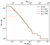 |
Fig. 1 Results from Test 1. Input cumulative mass function (green line) compared to ASOHF results with Nx = 64 (light red), Nx = 128 (red), and Nx = 256 (dark red). The vertical lines mark the completeness limit, at 90%, of the catalogue produced by ASOHF. This value is not reported with Nx = 256 because the code is able to detect all haloes. |
Completeness limits of ASOHF halo finding for Test 1 (in mass and number of particles, Mlim and  , at 90%.
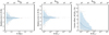 |
Fig. 2 Precision of ASOHF in recovering basic halo properties in Test 1, with Nx = 256. In each panel, dots represent individual haloes, the blue line presents the smoothed trend by using a moving median, and the shaded region encloses the 2σ confidence interval around it. Left panel: relative error in the determination of the virial radius. Middle panel: relative error in the determination of the virial mass. Right panel: centre offset, in units of the virial radius. |
3.2 Test 2. Substructure
To assess the ability of the code to detect substructure, we designed a second test consisting of a large, massive halo rich in substructure, with a similar procedure as in the previous test. In particular, we considered the same domain and cosmology, and placed a halo with a mass of 1015 M⊙ in its centre. In order to being able to span a wide range in substructure masses, we used Npart = 5123 DM particles, each with a mass of mp = 1.9 × 10⁷ M⊙. The particles in this host halo were generated in the same way as in Test 1, up to 1.5 Rvir.
Subsequently, we placed Nsubs = 2000 substructures, with masses drawn from the same Tinker et al. (2008) mass function, from Mmin = 50 mp = 9.4 × 10⁸ M⊙ and constraining the sample to have at least one large subhalo, with mass above 1013 M⊙. Sub-haloes were placed uniformly inside the host volume, avoiding overlaps, and were populated with particles following the same procedure as for isolated haloes. These particles were superimposed on the particle distribution of the host. The remaining particles up to Npart were placed outside the host halo by sampling a uniform random distribution to constitute a homogeneous background. It is worth stressing that even though the particles of each halo were sampled from a spherically symmetric NFW profile, the resulting realisation of the halo can depart strongly from spherical symmetry due to sample variance (especially relevant in smaller haloes, which are the most abundant). Therefore, the test contains many non-spherical haloes, including elongated systems that might resemble tidally stripped haloes.
We ran ASOHF on this particle distribution using a base grid of Nx = 512 cells in each direction and nℓ = 1 and 2 refinement levels, with a threshold of  particles per cell to flag it as refinable and accepting all patches with at least
  cells in each direction. The results for the detection capabilities of ASOHF are shown in Fig. 3. The input and recovered mass functions visually overlap, therefore the results are better assessed in the bottom panel, which shows their quotient. In general terms, just one refinement level allows detecting 95% of the substructures, while using two levels for the mesh increases this fraction to over 98%. At a more restrictive value of α = 0.99, the completeness limits correspond to ~270 and 55 particles for nℓ = 1 and 2, respectively. Even at a more restrictive threshold, these values are better than those in Test 1 (Table 2) because of the dense environment into which the substructures are embedded. This triggers the refinement of these regions more easily.
Figure 4 presents a thin (~46O kpc) slice of the density field as computed by ASOHF in order to pre-identify haloes. The adaptiveness allows simultaneously capturing small substructures within the dense host halo while removing sampling noise in underdense regions, which would increase and unbalance the computational cost. Purple circles represent the extent of the substructure, that is, a sphere of radius RJ. We note that in contrast to the virial radius of isolated haloes, the Jacobi radius naturally depends on the location of the substructure within its host: the more central its position, the smaller RJ in relation to the input virial radius of the NFW halo. This is quantitatively shown in Fig. 5, whose upper panel presents the relation between the input virial radius and the Jacobi radius determined by ASOHF. The trend implies that a satellite moving through a host would present a pseudo-evolution of RJ (and its enclosed mass) even if it moved rigidly through the medium (the smaller the distance to the host, the smaller RJ) While approximate due to the spherical symmetry and Keplerian rotation assumptions, this definition for the boundary of a substructure is reasonable because during the dynamical evolution of the infall of a satellite, it is expected that the particles in the outer layers become unbound through dynamical friction with the host particles. For more detailed studies, the whole list of particles of the satellite before its infall can be tracked (similarly to e.g. Tormen et al. 2004). In the lower panel, we show the tight linear correlation between the ratio of radii, RJ/Rvir,and the distance to the host centre,  This can be parametrised roughly as
 (4)
(4)
although the parameters naturally depend on the particular density profile of the host, and the scatter would be increased by the asphericity of real haloes.
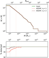 |
Fig. 3 Results from Test 2. Upper panel: input substructure cumulative mass function (green line) compared to ASOHF results with nℓ = 1 (red) and nℓ = 2 (dark red). The vertical lines mark the completeness limit, this time at 99%, of the catalogue produced by ASOHF. Bottom panel: fraction of substructures with input mass higher than M detected by ASOHF, with the same colour codes as above. |
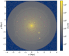 |
Fig. 4 Projection, 460 kpc thick, of the DM density field interpolated by ASOHF in Test 2, from which the pre-identification of haloes over the AMR grids is performed. The plot shows the maximum value in the projection direction. The black circle marks the virial radius of the host halo, and each purple circle corresponds to a substructure identified by ASOHF. The radius of each circle matches the Jacobi radius of the subhalo. |
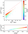 |
Fig. 5 Relation between virial and Jacobi radii in Test 2. Top panel: comparison between the virial radius of the input NFW halo |


3.3 Test 3. Unbinding
The unbinding procedure is a critical step in all halo finders based on configuration space because the initial assignment of particles has neglected any dynamical information. Here we present two tests to prove the capabilities of the two complementary unbinding procedures implemented in ASOHF: in Sect. 3.3.1 we study the case of a small halo moving in a dense medium, and in Sect. 3.3.2 we consider a fast stream traversing a halo.
3.3.1 Test 3a. Halo Moving in a Dense Medium at Rest
We considered a set-up similar to Test 1 (Sect. 3.1) in terms of box size and number of particles. We placed a halo of virial mass Mh = 5 × 10¹³ M⊙ in the centre of the box, and realised it with particles up to a radial distance of 3 Rvir ≈ 2.9 Mpc. This involved 73 976 particles, which are referred to as halo particles; 41 428 of them lie inside the virial radius.
The remaining ~2 × 10⁶ particles, corresponding to most of the mass in the box, were then placed in uniformly random positions in a sphere of radius 6 Rvir and are referred to as background particles. This amounts to a background of constant density ~75ρB, so that the halo and background densities are approximately equal at the virial radius of the cluster. Therefore, roughly one-fifth of the particles inside the virial volume are background particles. This may bias many of the halo properties (centre of mass position, bulk velocity, angular momentum, etc.).
We gave the halo particles a bulk velocity of 3000 km s−1 along the x-axis, so that background particles should be clearly unbound to the halo, and all particles (halo and background) were given a normal velocity dispersion with standard deviation of 300 km s−1 to add some noise. We note that it is not the aim of this test to use physically realistic values, but just to show the robustness and performance of the unbinding procedure in a fairly reasonable situation.
Figure 6 summarises the set-up and the results of the test. Its left panel shows the density profiles of the halo particles (blue) and of background particles (pink), which roughly agree with each other at the virial radius of the halo. The central panel in Fig. 6 presents the υz − υx phase space with the same colour code and shows that these two components are entirely disentangled in velocity space, but are mixed up in configuration space. Finally, the right panel shows the υrel − r phase plot, where υrel ≡ |υ − υhalo|, which corresponds to the space in which the escape velocity unbinding is performed. In this plot, the dashed purple line represents the local escape velocity at the last iterative unbinding step (when no more new particles are unbound), and the solid purple line is twice this value (which is the last threshold speed used for the escape velocity unbinding, according to the procedure described in Sect. 2.3). The particle-wise results in particular are described below.
The offset between the input centre and the centre detected by ASOHF is |Δr| = 2.3 kpc, which is 2.3%o of the virial radius (or 1.5% of the scale radius of the NFW profile). This small mis-centrering causes a decrease of 1.3%o in the virial radius of the host. Two halo particles that were nominally outside the halo are listed as inside, while 29 inside particles appear to be outside.
All background particles were pruned by one of the unbinding methods. Almost all background particles inside the virial volume (all but six) were pruned by the local escape velocity method, as shown by the fact that they lie above the threshold value 2υesc(r) (solid purple line) in the right panel of Fig. 6. It is worth noting that the iterative procedure of lowering the threshold, as described in Sect. 2, is crucial to prevent a biased centre-of-mass velocity in the first unbinding steps. The remaining six particles were pruned by the non-local unbinding in velocity space because they lie at more than 3συ of the centre-of-mass velocity. This method is especially useful for unbound components at small halo-centric distances because escape velocities are high near the halo core. Only one halo particle was incorrectly pruned, for being slightly over 3συ of the mean velocity.
This shows the ability of ASOHF of pruning the unbound component of haloes, even when it represents a significant amount of the mass within the halo volume. It also illustrates the situation of a satellite moving through its host. We note that a crucial step to enable unbinding host particles using the iterative procedure described in Sect. 2.3 is that the mass density of halo particles within the radial extent of the halo or satellite is greater than that of background or host particles. Otherwise, the centre-of-mass velocity would converge to that of the background. However, in the case of substructures, this condition is automatically guaranteed by the definition of the Jacobi radius (note that Eq. (2) implies that the substructure is at least three times denser than the mean density of the host within a sphere of radius D).
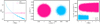 |
Fig. 6 Results from Test 3a (unbinding). Left panel: density profile of halo particles (blue) and background particles (pink). The dashed vertical line marks the input virial radius of the halo. Middle panel: υz − υx phase space, using the same colour coding as in the previous panel. The particle distributions are disjoint in velocity space. Right panel: υrei − r phase plot in which the unbinding is performed. The same colour coding as in the previous panels is used, the vertical line marks the input virial radius, and the dashed and solid purple lines are υesc(r) and 2υesc(r) at the last iteration of the local velocity speed unbinding, the latter being the threshold velocity for unbinding. |
3.3.2 Test 3b. Fast Stream Traversing a Halo
To illustrate the importance of the complementary velocity space unbinding, we present here a second test, in which a fast stream traverses a halo at rest. The set-up is as follows. A halo of virial mass Mvir = 1015 M⊙ is placed in the centre of a box, using the same particle mass (mp ≈ 1.2 × 10⁹ M⊙) as in the previous test. The halo is realised up to 3 Rvir with ~1.5 × 10⁶ particles (the halo particles). As for the stream of particles, we considered a curved cylindrical stream, with impact parameter b = 0.5 Rvir, curvature radius r = 2 Rvir, radius Δb = 250 kpc, and length L ≈ 8.3 Mpc (so that it crosses the whole virial volume of the halo). We assigned a density of 200ρB to the stream, so that it amounts to a mass of 1.29 × 10¹³M⊙, or slightly over 10000 particles (the stream particles). The situation in configuration space is depicted in the left panel of Fig. 7, where blue (pink) dots represent the x - z positions of halo particles (stream particles) lying within a 20 kpc slice passing through the centre of the halo.
Velocities for the halo particles were drawn from a normal distribution with zero mean and an isotropic σ1D = 300 kms−1. Stream particles were given a speed of 3000 km s−1 along the axis of the stream, plus an isotropic dispersion component as in the halo particles. The middle panel of Fig. 7 shows that while most of the stream particles are nominally unbound, (υ > υesc(r)), they do not reach the threshold for unbinding, 2vesc. While lowering this threshold would remove these particles, loosely unbound particles (i.e. those with vesc(r) < v < 2vesc(r)) may still remain within the halo for a dynamical time. This means that lowering the threshold is somewhat aggressive (see also the discussion in Knebe et al. 2013 and Elahi et al. 2019).
However, the situation in velocity space clearly presents two disjoint components, as represented in the right panel of Fig. 7. In this case, the velocity space unbinding is able to remove all stream particles because they lie beyond 3σv of the centre-of-mass velocity after the iterative procedure.
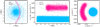 |
Fig. 7 Results from Test 3b (unbinding). Left panel: particles in a 20 kpc slice through the centre of the halo. Blue (pink) dots refer to halo (stream) particles. The dashed grey circle corresponds to the location of the input virial radius. Middle panel: vral – r phase plot, with the same colour coding as in the previous panel, showing that the local escape velocity unbinding does not succeed in pruning the stream. Right panel: vz – vx phase space, keeping the colour coding as in the previous plots. The purple cross, dashed circle, and solid circle indicate the converged centre-of-mass velocity and the 1σv and 3σv regions, respectively. Particles outside the latter are pruned by the velocity space unbinding. |
3.4 Scalability
While the previous set of tests demonstrates the ability of ASOHF to provide complete samples of haloes with unbiased properties, here we consider the performance of the code in terms of execution time and memory requirements in more detail. We used a set-up similar to that of Test 1 to assess how the code scales with the number of particles and base grid size (Sect. 3.4.1), and the performance increase with the number of OMP threads (Sect. 3.4.2). All the results given here correspond to the performance of ASOHF on a Ryzen Threadripper 3960X processor with 24 physical cores.
3.4.1 Scaling with Npart and Nx
To assess the scaling capabilities of the code with increasing number of particles and size of the base grid, we replicated the set-up in Test 1 (Sect. 3.1) with varying number of particles. To do this, we first considered the case with the largest number of particles, Npart = 10243 (corresponding to a particle mass of  ) and generated and randomly placed 366652 haloes with masses higher than
  Then, we realised this halo catalogue with Npart = 323, 643, etc. up to 10243 DM particles. For each realisation, we only kept the haloes with masses higher than or equal to that corresponding to 50 particles. For each value of Npart, we tested
  and
and 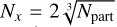 11 because Test 1 (Sect. 3.1) showed that this latter value was able to recover all haloes. For the AMR grid parameters, we used
  , and the remaining parameters were kept as in Test 1. The detailed results are presented in Table 3 and are graphically summarised in Fig. 8.
The left panel in Fig. 8 shows the scaling of the 90% mass completeness limit with the number of particles for the two base grid sizes ( in dark red, labelled ‘a’ in Table 3; and
  in light red, labelled ‘b’; the same colour code is kept in the remaining panels). The dashed grey lines are lines of constant number of particles (at fixed total mass in the box), so that it is explicitly shown that using
  (runs a) the code is able to correctly identify barely all haloes comprising more than ~140 particles. For the runs b, with
  all haloes were detected and the completeness limit is arbitrarily placed at the minimum mass of the input mass function (50 particles) for representation purposes. Nevertheless, it is worth stressing that in real situations, where an LSS component surrounds the haloes, it is not generally necessary to increase the base grid resolution beyond
  to detect more smaller haloes, although this may be useful for some particular applications (e.g. identifying haloes within voids).
The wall time taken by each of the runs is presented in the central panel of Fig. 8. Runs 4.1, 4.2, and 4.3, with fewer than one million particles, last for less than a few seconds. These results are therefore biased with respect to the general scaling because the measured times are likely to be dominated by input-output, system tasks, and by the coarse time resolution of the profiling utility used. For large enough task sizes (i.e. for Npart≳ 2563), the wall time increases proportionally to the product Npart☓Nhaloes, as shown by the dashed lines, which correspond to constant time per halo and particle. When the base grid resolution is increased from  to
to  the scaling is kept, but the normalisation of the relation increases by a factor of 2–3, mostly associated with the fact that more haloes are detected in this case (both real haloes and spurious peaks throughout the interpolated density field, which are later discarded when particles are considered).
The right panel in Fig. 8 depicts the peak memory requirements of the code. When the grid size is fixed at  , ASOHF requires ~180–200 bytes/particle, which allows running the code on desktop-sized workstations for simulations with up to hundreds of millions of particles. When the base grid resolution is doubled, these memory requirements increase up to ~1 kbyte/particle.
Last, we note that as the number of particles increases, the scaling  can greatly benefit from performing a domain decomposition for running ASOHF, as described in Sect. 2.6.1. This is especially useful in large domains, where the required overlaps amongst domains (which can be as low as the size of the largest expected halo) correspond to a negligible fraction of the volume. Therefore, when the volume is decomposed in d domains, the CPU time is reduced by a factor d, since the number of particles and haloes in each domain are themselves reduced by a factor d, on average. If all domains can be run concurrently, rather than sequentially, this amounts to an improvement in wall time of a factor of d2.
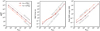 |
Fig. 8 Summary of the results from the scalability test (Sect. 3.4.1). Left panel: scaling of the 90% completeness limit (in terms of mass) with the number of particles in the domain. Dashed grey lines correspond to a constant number of particles. Dark red (light red) lines represent the results for the two base grid sizes according to the legend. Middle panel: scaling of the wall time taken by ASOHF with number of particles. Dashed grey lines correspond to a scaling |

Results of the scalability tests.
3.4.2 Scaling With the Number of Threads
To explore the performance gain in terms of wall time and memory usage of the OMP parallelisation scheme, we repeated Test 4.5a (see Table 3) with ncores = 1, 2, 4, 8, 16, 24, and 32 and 36 OMP threads using nodes equipped with two 18-core CPU Intel® Xeon® Gold 6154. The results are presented in Fig. 9.
The upper panel exemplifies the performance improvement when the number of cores is increased. Red crosses correspond to the actual performance of ASOHF with a varying number of threads. We fitted these data to the functional form
 (5)
(5)
using a least-squares method, finding that the sequential part amounts for  min, while the parallel part would correspond to a CPU time of
  . Being
  the scaling of the code is close to optimal (null sequential part, which is represented by the green line in the upper panel of Fig. 9) for ncores≳ 100, which is a reasonably high number of threads available in typical shared memory nodes. The exponent α resulting from the fit is α = 1.007 ± 0.017 ≊ 1, which is consistent with the expected behaviour of the parallel part. It is interesting to note the absence of a significant performance gain when increasing from 16 to 24 cores because the system is comprised of two non-uniform memory access (NUMA) nodes, with 18 physical cores each. When the treads are increased from 16 to 24, the task can no longer be allocated to a single node, so that memory access outside the node is penalised. This is a well-known issue in shared-memory systems, and we advise the interested users to take the architecture of their system into account for optimal performance.
However, increasing the number of OMP threads implies an increased memory usage because it is necessary to replicate part of the data. The lower panel in Fig. 9 displays the (linear) relation between the number of threads and the peak RAM used by the job. To conclude this section, we recall that these results are dependent on the application and the configuration. For example, it is reasonable to expect a smaller memory penalty by increasing the number of threads in simulations of large volumes, where each halo contains only a small fraction of the particles in the domain, as opposed to these test cases, in which a halo contains nearly 25% of the particles.
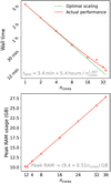 |
Fig. 9 Parallel performance of ASOHF. Upper panel: scaling of the wall time of ASOHF in Test 4.5a (see Table 3) when the number of OMP threads is varied. The solid red line is a fit of the benchmark data (red crosses), and the dashed green line corresponds to an optimal scaling i.e. twall ∝ 1 /ncores. Lower panel: peak memory usage of ASOHF scaling with the number of OMP threads. |
4 Tests on Real Simulation Data and Comparison with Other Halo Finders
Last, in order to evaluate the performance of ASOHF on a cosmological simulation, we have tested our code on outputs from the public suite CAMELS (Villaescusa-Navarro et al. 2021, 2022). The Cosmology and Astrophysics with MachinE Learning Simulations project consists of over 4000 simulations of (25h–1Mpc)3 ≈ (37.25 Mpc)3 cubic domains, including DM-only and (magneto)hydrodynamic (MHD) simulations with star formation and feedback mechanisms, and covering a broad space of several cosmological and astrophysical parameters. Alongside with the simulation data, the public release also includes halo catalogues produced with three public halo finders, namely SUBFIND (Springel et al. 2001; Dolag et al. 2009), AHF (Gill et al. 2004; Knollmann & Knebe 2009), and R0CKSTAR (Behroozi et al. 2013), which we use here to examine how does ASOHF compare to other well-known halo finders.
In particular, we used the simulation LH–1 from the IllustrisTNG subset of CAMELS. These simulations were carried out using Arepo (Springel 2010; Weinberger et al. 2020), which is a publicly available code using a tree+particle-mesh (TreePM) scheme coupled to Voronoi moving-mesh MHD for hydrodynamical cosmological simulations, including galaxy formation physics. The TreePM (Bagla 2002) method implemented in Arepo, which combines a particle-mesh method for computing the large-range force with a more accurate tree code (Barnes & Hut 1986) at short distances, allows these simulations to host very many small haloes and substructures even though the number of DM particles,  is modest. The comoving gravitational softening length is as low as 2 kpc. While all CAMELS simulations correspond to flat universes with a baryon density parameter Ωb = 0.049, Hubble constant h = H0/(100kms–1 Mpc–1) = 0.6711, and spectral index ns = 0.9624, the simulation we chose, name-coded LH–1, assumes a matter density parameter Ωm = 0.3026 and σ8 = 0.9394 as the amplitude of the primordial fluctuations spectrum. These parameters imply a DM particle mass of mpart = 9.8 x 10⁷ M⊙.
4.1 Results Analysing only DM Particles
We ran ASOHF using only DM particles on the most recent snapshot of this simulation (at redshift z = 0), using a base grid with as many cells as particles (Nx = 256) and nℓ = 6 refinement levels, so that the peak resolution of the grid is ∆x6 ≈ 2.3 kpc, similar to the gravitational softening length of the simulation. The threshold particle number to mark a cell as refinable was set to 3, and the minimum patch size was set to 14 cells. Density was interpolated with a kernel size determined by the local density, using four kernel levels. We discarded all haloes resolved with fewer than 15 particles. In this configuration, ASOHF detects 11794 non-substructure haloes, the most massive of them with a DM mass of 7.44 × 10¹³M⊙, and 1263 substructures (including sub-substructures). The wall-time duration of the test was below 4 min, using eight cores in the same architecture as described in Sect. 3.4.1.
The halo mass function recovered by ASOHF is shown as the solid thick red line in the upper panel of Fig. 10, together with the same quantity obtained from the catalogues of AHF (solid blue), Rockstar (solid green), and Subfind (solid orange). For reference, the thick pale purple line represents a reference Tinker et al. (2008) mass function with the cosmological parameters of the simulation. At first glance, all four halo finders yield comparable mass functions (both amongst them and with the reference one) for Npart ≳ 1000, with some variations at the high-mass end due to the combination of small number counts and subtleties in the mass definitions.
To allow a more precise comparison, the lower panel presents each of the mass functions, normalised to the geometric mean of all four finders, which we take as the baseline for comparison. In this plot, the red line (corresponding to ASOHF) displays the Poisson  confidence intervals as the shadowed red area. The magnitude of these uncertainties is similar for the other lines. ASOHF, Subfind, and Rockstar match reasonably well inside their respective confidence intervals, while AHF shows a small ≳15% excess with respect to them at Npart ~ 104. Interestingly, Rockstar and ASOHF present the largest similarities in their mass function. They match each other within a few percents all the way down to 50–100 particles, when ASOHF starts to identify a larger number of structures. Compared to them, Subfind starts to present a larger abundance of haloes below Npart ≲ 1000, mostly driven by the larger number of substructures, while the AHF halo counts stall below a few hundred particles.
Dashed lines in the upper panel of Fig. 10 present the substructure mass functions for the four halo finders, using the same colour code. In this case, substructure mass functions are not so easily comparable, and thus the differences amongst the finders are exacerbated (see e.g. Onions et al. 2013). In particular, Subfind finds the largest number of substructure, nearly 2.5 times as many as ASOHF, 6 times more than Rockstar and 30 times more than AHF. Even the high-mass end of the subhalo mass function shows important differences, with Subfind having the highest and ASOHF the lowest mass of their respective most massive substructure. This is mainly due to the fundamentally different definitions of substructure. The ASOHF choice of using the Jacobi radius, which approximately delimits the region in which the gravitational attraction of the substructure is stronger than that of the host, is more restrictive than other definitions, for example, using density contours traced by the AMR grid (AHF), reducing the 6D linking-length (Rockstar), or finding the saddle point of the density field (Subfind). This more stringent definition of the substructure extent may indeed also be the reason that ASOHF recovers less substructure than Subfind because many of the small substructures identified by the latter may contain fewer than 15 particles using our more stringent definition based on the Jacobi radius.
Focusing on the main properties of haloes, in Fig. 11 we present the comparison of ASOHF radii and masses to the corresponding magnitudes obtained by AHF (left column), Rockstar (middle column), and Subfind (right column). For each halo finder, we first matched its catalogue to the catalogue produced by ASOHF. Here, we only focus on haloes and exclude substructure because, as mentioned above, the substructure definitions of each algorithm are fundamentally different. The results are also summarised in Table 4.
Surprisingly, and despite their agreement regarding the mass functions, we are only able to match ~20% of Rockstar haloes to ASOHF’s12, in contrast to ~80% of matches when comparing to AHF and Subfind. For each property, X, that is to be compared, we fitted the matched data to a power law of the form
 (6)
(6)
where N is the normalisation and α is the index (both are unity if the finders yielded identical results). X* is a normalisation for the quantities, which we selected as the median over the ASOHF sample: R* = 43.2kpc and M* = 5.18 × 10⁹ M⊙. For each fit, we computed the scatter as the RMS of the relative residuals between the data points and the fit,
 (7)
(7)
where  is the fitting function from Eq. (6) with the best parameters obtained by least-squares estimation.
The largest discrepancies with ASOHF are seen when it is compared to AHF, which overall finds ~6% larger radii than ASOHF. This may be well due to the fact that AHF uses all particles (including gas and stars) to determine the spherical overdensity radius, while we only use DM particles. This normalisation offset in radii propagates to a ~22% offset in masses. There is a significant amount of scatter in radii and masses at the low-mass end, with a population of matched haloes with AHF radii a few times that of ASOHF. This is not seen when comparing with the rest of halo finders.
Although only ~1200 haloes are matched between Rockstar and ASOHF catalogues, their virial radii and masses match tightly, with ~4 and 5% offsets, respectively. A few outliers increase the overall scatter figure, which reaches ~5 and ~16% for radii and masses, respectively. When they are excluded, the relation is quite tight.
Strikingly, despite their very different natures, the Subfind results are the most compatible with ASOHF of the halo finders we considered. With almost 8000 matched haloes, the normalisations as defined in Eq. (6) only show a 1% offset in radii and a 3% offset in mass. The scatter, dominated by the low-mass haloes, is 2.5 and 8%, respectively.
Overall, and despite the difficulties of comparing results of different halo finders on a halo-to-halo basis, which has been thoroughly explored in the literature (see Knebe et al. 2011, 2013; Onions et al. 2012), these analyses show that ASOHF is capable of providing results that generally agree well with other widely used halo finders. The largest discrepancies are seen at the smallest scales.
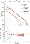 |
Fig. 10 Comparison of the mass functions of the halo catalogues obtained by ASOHF (red), AHF (blue), Rockstar (green), and Subfind (orange) in the CAMELS Illustris–TNG LH–1 simulation at z = 0. Upper panel: mass functions obtained by each code, as solid lines. The thick purple line corresponds to a Tinker et al. (2008) mass function at z = 0 and with the cosmological parameters of the simulation for reference. Dashed lines present the mass function of subhaloes in the same colour scale. Lower panel: mass function of non-substructure haloes, normalised by the geometric mean of this statistic for the four halo finders. The shadow on the red line (ASOHF) corresponds to |

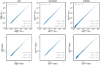 |
Fig. 11 Comparison of the main properties (masses, top row; and radii, bottom row) of the matched haloes between ASOHF and AHF (left column), Rockstar (middle column), and Subf ind (right column). For the two latter we compare virial radii and masses, and for the former, we use R200c and M200c because the AHF catalogues given in the public release of CAMELS have used this overdensity for marking the boundary of the halo. |
Summary of the main features of the comparison between ASOHF, AHF, Rockstar, and Subfind.
4.2 Results Including Stellar Particles
By the last snapshot, at z = 0, the simulation contains 227 454 stellar and black hole (BH) particles, accounting for ~2%0 of the DM mass in the computational domain. While the mass in stars is too low to significantly impact the process of halo finding (by enhancing DM density peaks that would otherwise be too small to be detected), we can still demonstrate the ability of ASOHF of characterising stellar haloes.
We ran ASOHF on the DM+stellar particles of the same simulation and snapshot as considered above and kept the same values for the mesh creation and DM halo-finding parameters. The stellar halo-finding parameters, which as discussed in Sect. 2.5 do not affect the resulting galaxy catalogues strongly, were set such that all stellar haloes with more than  = 15 stellar particles inside the half-mass radius were kept. We preliminarily cut the stellar haloes whenever the density increased by more than a factor fmin = 5 from the profile minimum, there was a radial gap of more than ℓgap = l0kpc without any stellar particle or stellar density fell below the background density, ρB(z) (fB = 1).
In this configuration, ASOHF identifies 337 stellar haloes, with masses ranging between 1.1 × 10⁸M⊙ and 1.5 × 10¹¹M⊙, and whose cumulative mass distribution is shown in Fig. 12 by a red line (here, Mgal makes reference to the stellar mass inside the stellar half-mass radius, defined in Sect. 2.5). The dashed green line presents a fit to a Schechter (1976) function. The fit was performed over the differential mass function, and obtained a chi-squared per degree of freedom  (computed assuming Poissonian errors for number counts). This implies that the fit is not inconsistent with a Schechter (1976) mass function.
An example of such an identification is represented graphically in Fig. 13. In this figure, the background colour encodes the DM+stellar projected density in grey scale, as computed by ASOHF, around the most massive DM halo in the simulation (which is a ~8 × 10¹³M⊙ group). Each colour represents all the particles of a given stellar halo. A central halo, represented in turquoise, dominates the stellar mass budget. This halo has a half-mass stellar radius of ~36kpc, whose extent is represented as the dashed white circle in the figure, around a white cross marking the stellar density peak. Around it, ASOHF detects ten satellite haloes, each represented in a different colour. In dark blue, we plot all the particles inside the virial volume of the main DM halo that do not belong to any stellar halo. Although a few groups of stars on top of some DM haloes that are not identified as galaxies are visible, these objects correspond to poor stellar haloes, with fewer than 15 stellar particles. They were therefore discarded by ASOHF.
We summarise some of the properties of the stellar haloes catalogue in Fig. 14. The left panel contains a histogram of the half-mass stellar radii. The distribution of galaxy sizes peaks at around (6–8) kpc, while a handful of haloes as large as R1/2 ≳ 20kpc are found, most typically associated with massive DM haloes. Although more rare, some of them correspond to small (~1011M⊙) DM haloes with an extended stellar component.
In the middle panel of Fig. 14, we present the relation of stellar mass inside the half-mass radius (vertical axis) to DM host halo mass (horizontal axis). For reference, we indicate some constant stellar fractions as grey lines. At low stellar mass (M*.,1/2 ≲ 2 ×10⁹), we find a large scatter between stellar and DM halo masses. The relation becomes tighter at high stellar halo masses, approaching but not reaching 1%. The particularities of these results may have to do with the particular IllustrisTNG feedback scheme implemented in the simulation and numerical resolution. Discussing them is beyond the scope of this work.
Last, the right panel of Fig. 14 contains the stellar 3D velocity dispersion correlated to the stellar mass of the halo. This relation shows a clear increasing trend because more massive haloes (if virialised) have larger kinetic energy budgets or are dynamically hotter. This result provides a dynamical confirmation of the fact that our galaxy identification scheme targets bona fide stellar haloes and not spurious groups of particles. In sum, with these examples, we show the capabilities of ASOHF, not only as DM halo finder, but also as a galaxy finder for cosmological simulations.
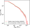 |
Fig. 12 Mass function of stellar haloes found in the simulation from CAMELS at z = 0 (red line). The mass of the galaxy on the horizontal axis, Mgal, refers to the stellar mass inside the half-mass radius of the stellar halo. The red shading represents the Poissonian, |

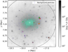 |
Fig. 13 Example of the stellar halo finding capabilities of ASOHF. The background greyscale colour map is a projection of DM+stellar density around the most massive halo in the simulation. The solid black line indicates its virial radius. The coloured dots correspond to stellar particles, and each colour corresponds to a different stellar halo. The dark blue dots are the particles inside the virial volume of the DM halo that do not belong to any identified stellar structure. For the central galaxy, the white cross and circle represent the stellar density peak (which we regard as centre) and the half-mass radius of the stellar halo, respectively. |
5 Conclusions
We have introduced and discussed a revised version of the DM halo finder ASOHF, which constitutes a profound revision of most of the features of the original version that was presented over a decade ago by Planelles & Quilis (2010). The ever-increasing trend in cosmological simulation sizes and resolution, and the accordingly greater abundance and richness of structures at a wide range of scales, required revisiting several aspects related to the halo-finding process. Because they are the basic building blocks of the LSS of the Universe, an exceptionally precise characterisation of DM haloes is a mandatory condition for bridging the gap between simulations and observations and bringing cosmological predictions from simulations to accuracies below the percent level (e.g. Borgani 2008; Clerc & Finoguenov 2022, for several reviews about cluster cosmology), especially when the smallest scales are involved (e.g. Vogelsberger et al. 2020, and references therein). Related to this, given that the baryonic processes leading to galaxy formation are being exhaustively analysed in numerical works (e.g. Murante et al. 2010; Iannuzzi & Dolag 2012; Vogelsberger et al. 2014; Schaye et al. 2015; Kaviraj et al. 2017; Pillepich et al. 2018; Villaescusa-Navarro et al. 2021, for some large galaxy formation simulation projects), it is of the utmost importance to devise numerical techniques to describe them accurately.
Amongst the main improvements to the halo-finding procedure that were assessed in a battery of complex, idealised tests and in a cosmological simulation, we summarise the main points below. They can be useful not only for ASOHF, but for halo finders in general (especially for those that are based on configuration space).
-
The density interpolation procedure is, naturally, critical to the procedure of halo finding because an overly smoothed interpolation would accidentally smear true density peaks, thus losing small-scale structures, while a density interpolation that is too sharp (e.g. applying a CIC or TSC at the resolution of each grid) increases the computational cost of the process dramatically by producing a large number of spurious peaks due to sampling noise. A compromise between these extremes is achieved by spreading particles in a cloud, whose size can be tuned either by local density or by particle mass (i.e. by the volume sampled by the particle in the initial conditions), but is independent of the grid level. Nevertheless, since any interpolation will tend to be more diffuse than the particle distribution itself, it is generally harmless to also consider density peaks above a certain fraction of ∆vir(z) as candidates for halo centres.
Because the grid resolution is finite (one cell can contain thousands of particles even at the finest levels for very cuspy haloes), the implementation of a recentring scheme (using information at finer levels, and ultimately using the particle distribution to iteratively relocate the local maximum of the density field) is crucial to avoid centre offsets. Preventing this erroneous centring is critical to describe the properties of the inner regions of haloes.
While the local escape velocity unbinding that is implemented in many halo finders is successful in removing physically unbound particles, the fact that a conservative threshold (e.g. 2vesc) is normally used can make it insufficient in some occasions. This can be improved by an additional unbinding scheme in pure velocity space, which proves useful to disentangle dynamically unrelated particles from the halo (see the examples in Sect. 3.3, especially Fig. 7).
The new version of ASOHF implements an entirely new scheme for searching for substructure that is different from the search for isolated haloes. In our experiments, we find that delimiting substructures by their density profile (e.g. placing a radial cut when the spherically averaged density profile increases) leads to too generous radii, which therefore contaminate the mean velocity of the halo and can degrade the performance of unbinding and even miss the halo. In ASOHF, density peaks located within the volume of previously identified haloes, at finer levels of refinement, are characterised by their Jacobi radius, which approximately delimits the region in which the gravitational force towards the substructure centre is dominates that of the host. In addition to its clear physical motivation, this (typically more stringent) radius together with the improved unbinding scheme helps to avoid the bias in the halo properties.
Using the DM haloes, ASOHF is able to identify and characterise stellar haloes, that is, galaxies. While the starting point for this identification is the catalogue of DM haloes and subhaloes, the stellar haloes are subsequently treated as independent objects. In particular, they can have a different centre, radial extent, dynamics, and so on than the DM halo they are built onto.
We have implemented a domain decomposition for ASOHF that enables the analysis of large simulations that would otherwise not fit in memory. Incidentally, as discussed in Sects. 2.6.1 and 3.4.1, the domain decomposition also strongly reduces the CPU time. Furthermore, the procedure is implemented by external, automated scripts, and each domain can be treated as a separate job (requiring no communication). This means that different domains can be either run concurrently (so that the wall time is reduced by a factor equal to the number of cores) or sequentially. The resulting outputs for each domain can be merged by an independent script, so that the whole process is transparent to the user.
-
By saving the particle IDs of all the bound particles of each halo, the merger tree can easily be built once the catalogues have been obtained for (at least) a pair of code outputs.
This process is dramatically accelerated by pre-sorting the lists of particles by ID, and thus intersecting them in O(N) operations, instead of O(N2). Building the merger tree as a separate task from the halo-finding procedure has several benefits, such as avoiding the need to overload the memory with all the information of previous iterations, or the ability to connect a halo with a progenitor skipping iterations, if it has not been found in the immediately previous iteration. There are also drawbacks of this approach: for instance, the inability to incorporate the merger tree information into the halo finding process itself, such as other modern finders do (e.g. HBT+; Han et al. 2018).
Through a battery of tests described in Sect. 3, we have shown the ASOHF capabilities of recovering virtually all haloes and subhaloes in a broad range of masses in idealised but complex set-ups. When compared to other publicly available halo finders, such as AHF, Rockstar, or Subfind, ASOHF produces comparable results in terms of halo mass functions and properties of haloes. It provides excellent results in terms of substructure identification (in the sense that it is able to identify a large number of substructures, while using a tight, physically motivated definition of substructure extent). This is commonly a tough task for SO halo finders when compared to 3D-FoF, but especially when compared to 6D-FoF finders.
Regarding computational performance, the new version of ASOHF has been rewritten to be extremely efficient in terms of speed, parallel scaling, and memory usage. As discussed in Sect. 3.4.2, the parallel behaviour of the code scales nearly ideally, which allows a large performance gain using shared-memory platforms with a large number of cores. Moreover, the optimisation of the code allows analysing individual snapshots from simulations of ≳107 particles within tens of seconds and using a few GB of RAM, and simulations with ≳ 108 particles within tens of minutes and using less than 30 GB of RAM in any case.
When large domains with an even larger number of particles are involved, the time taken by ASOHF can be further improved by the domain-decomposition strategy, which involves no communication between different domains until a last step at which catalogues are merged. As an example, for a simulation with ~1010 particles within a cubic domain with a side length of 500Mpc/h, where ~15 × 106 haloes are expected to form by z = 0, scaling the benchmarks characterised in Sect. 3.4.1 we estimate that by performing a decomposition in d = 43 sub-domains, ASOHF could run over all the domains (sequentially i.e. one domain at a time) in ~93 h of wall time, in a 24-core processor like the one used for the Tests in Sect. 3.4.1. If 8 of such nodes were concurrently available in a distributed memory architecture, this would take ≲12h. The implementation of ASOHF, together with the several utilities and scripts mentioned in this paper, is publicly available and documented13.
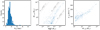 |
Fig. 14 Summary of some of the properties of the stellar haloes identified by ASOHF in the CAMELS, IllustrisTNG LH–1 simulation at z = 0. Left panel: distribution of half-mass radii. Middle panel: relation of stellar mass to DM halo mass. Diagonal lines correspond to constant stellar fractions. Right panel: relation of 3D velocity dispersion to stellar mass. |
Acknowledgements
We thank the anonymous referee for his/her constructive comments, which have improved the presentation of this work. This work has been supported by the Spanish Ministerio de Ciencia e Innovatión (MICINN, grant PID2019-107427GB-C33) and by the Generalitat Valenciana (grant PROMETEO/2019/071). D.V. acknowledges support from Universitat de Valencia through an Atracció de Talent fellowship. Part of the tests have been carried out with the supercomputer Lluís Vives at the Servei d’Informàtica of the Universitat de València. This research has made use of the following open-source packages: NumPy (Oliphant 2006), SciPy (Virtanen et al. 2020), Matplotlib (Hunter 2007), and Colossus (Diemer 2018).
Appendix A Solution of Poisson’s Equation in Spherical Symmetry
The local unbinding procedure, described in Sect. 2.3, relies on the computation of the gravitational potential in spherical symmetry. Here we describe our implementation of the procedure.
In general, the gravitational potential, Φ, of any continuous or discrete density distribution p is obtained by solving Poisson’s equation,
 (A.1)
(A.1)
which is an elliptic partial derivative equation, where r and x = r/a are the physical and the comoving position vectors, respectively, related by the expansion factor a(t) that solves Friedmann equations for a given cosmology. Under the assumption of spherical symmetry in the density distribution (and thus in the potential), the Poisson equation reduces to a non-linear second-order ordinary differential equation,
![Mathematical equation: $ {{\rm{d}} \over {{\rm{d}}r}}\left[ {{r^2}{{{\rm{d}}\Phi } \over {{\rm{d}}r}}} \right] = 4\pi G\rho \left( r \right){r^2}. $](/articles/aa/full_html/2022/08/aa43712-22/aa43712-22-eq103.png) (A.2)
(A.2)
If the mass distribution is bound, it is always possible to take lim r→∞Φ(r) = 0 and show that
 (A.3)
(A.3)
where  is the mass enclosed in a sphere of radius r. Assuming the mass distribution to be bound within a maximum radius rmax, it is then straightforward to rewrite this expression in a more convenient form for its numerical integration,
 (A.4)
(A.4)
Only the first term in Eq. A.4 is a function of r. Operationally, we use the following recipe to efficiently perform the integration.
Start from a list of npart particles (i = 1,…,npart), with masses
 , sorted in increasing comoving distance to the halo centre (density peak),
  . Denote
Compute the cumulative mass profile, which we denote

Identify
 as the smallest integer such that
  , and define
Compute iteratively, for
 , the value of
  at the position of the next particle as
  .
.Define the constant
 .
.The spherically symmetric gravitational potential at comoving radius ri is
 .
.
We perform step 3, that is, we assume a constant gravitational potential in the inner 1% of the radial space, to mitigate numerical errors since ri can be arbitrarily small. This has a negligible impact on the unbinding procedure because it is rare to find unbound particles near halo centres.
Appendix B Computation of the Gravitational Binding Energy by Sampling
The gravitational binding (or potential) energy of a system of N particles is explicitly given by the sum over all particle pairs:
 (B.1)
(B.1)
which therefore implies and O(N2) calculation, which becomes prohibitively expensive for large enough N. In ASOHF, we perform a direct summation over the N(N – 1)/2 pairs for haloes with  particles (see the discussion of Fig. B.1 for the dependence of the accuracy of the results on this parameter), while for larger haloes, we use a sampling estimate of this quantity, which we describe and test below.
In order to estimate the gravitational binding energy of large haloes by sampling, we consider  pairs of particles and compute the contributmiomn of each to the potential energy, that is,
  for the pair of particles (ij). The procedure is as follows:
First, we randomly select nsample particles (with replacement), which we denote i = 1, …, nsample. For each of these particles, we select a new set of nsample particles (with replacement), which we denote j = 1,… nsample, and compute for Carticle i its contribution to the gravitational energy,  The gravitational energy per pair of particles therefore is
 (B.2)
(B.2)
Since there are N(N – 1)/2 pairs of particles in the halo, we estimate its gravitational energy as
 (B.3)
(B.3)
We note that Egrav ∝〈Egrav, pairs〉 and thus the relative error in Egrav is equal to the relative error in 〈Egrav,pairs〉, which in turn is proportional to  and independent of N. This is graphically exemplified in Fig. B.1.
The gravitational binding energy per unit mass of particle i is proportional to Egrav,i/mi. Thus, we report as the most bound particle the particle with the most negative value of Egrav,i/mi, which can incidentally be used as an estimation of the location of the minimum of gravitational potential. The uncertainty in determining this position can be estimated as the sphere, with centre in the most-bound particle, that encloses [N/nsample] particles.
To assess the convergence of this method, we generated NFW haloes with an arbitrarily fixed concentration of c = 10 and radius R = 1.5 (in arbitrary units), realised using different numbers of particles, N, from 5 × 10⁴ to 106. We then computed the gravitational energy by direct O(N2) summation as in Eq. B.1, and by the sampling method varying nsample between 102 and 104. For each pair of values of (N, nsample), we performed nboots = 100 bootstrap iterations of the calculation by sampling, so that we can estimate the mean relative error in the gravitational potential energy by comparing with the result by direct summation, and its (16 – 84)% confidence intervals.
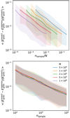 |
Fig. B.1 Dependence of the error in obtaining the gravitational binding energy by sampling, rather than by direct summation over all the pairs of particles, with the fraction nsample/N (upper panel) and with just the number of sample particles nsample (lower panel). The number of evaluated pairs of particles is |

This is shown in Fig. B.1, whose upper panel shows the mean of the relative error, computed over the 100 bootstrap iterations, in computing the gravitational energy by sampling. Each colour represents a different number of particles in the halo according to the legend in the lower panel, while on the horizontal axis, we show the fraction of nsample to N. For each N, the error clearly decreases as 1/ These curves can be brought to match each other when we represent the relative error as a function of nsample, as shown in the lower panel of Fig. B.l. In this case, regardless the number of particles of the halo, the mean errors fall below 1% when more than nsample ≈ 2000 are used, while nsample must be increased to ~ 5000 – 6000 to achieve an error below 1% at the 84 percentile.
It would be reasonable to ask why the error scales as  , instead of
  , which would be expected from averaging nparis values of the energy per pair of particles. This is due to the fact that we are considering nsample particles, and estimating the gravitational binding energy of each of these with a new set of nsample particles. This is fundamentally different from choosing npairs completely independent pairs, in which case it is easy to verify that the error indeed scales as ∝1/nsample However, this latter method, although much faster in terms of convergence (lower values of nsample are required, and the computational cost is therefore greatly reduced), does not allow us to estimate the most-bound particles of haloes (and therefore the position of the gravitational potential minima). This is so because to achieve this aim, we require a good estimate of the energies of a subsample of individual particles. This cannot be achieved by randomly picking pairs of particles because each particle will be considered a few times as much. We therefore opt in ASOHF for this more slowly converging method.
References
- Angulo, R. E., & Hahn, O. 2022, Liv. Rev. Comput. Astrophys., 8, 1 [CrossRef] [Google Scholar]
- Bagla, J. S. 2002, J. Astrophys. Astron., 23, 185 [NASA ADS] [CrossRef] [Google Scholar]
- Barnes, J., & Hut, P. 1986, Nature, 324, 446 [NASA ADS] [CrossRef] [Google Scholar]
- Behroozi, P. S., Wechsler, R. H., & Wu, H.-Y. 2013, ApJ, 762, 109 [NASA ADS] [CrossRef] [Google Scholar]
- Binney, J., & Tremaine, S. 1987, Galactic dynamics, Princeton Series in Astrophysics (Princeton: Princeton University Press) [Google Scholar]
- Borgani, S. 2008, in A Pan-Chromatic View of Clusters of Galaxies and the Large-Scale Structure, eds. M. Plionis, O. López-Cruz, & D. Hughes (Berlin: Springer), 740, 24 [Google Scholar]
- Bryan, G. L., & Norman, M. L. 1998, ApJ, 495, 80 [NASA ADS] [CrossRef] [Google Scholar]
- Cañas, R., Elahi, P. J., Welker, C., et al. 2019, MNRAS, 482, 2039 [CrossRef] [Google Scholar]
- Clerc, N., & Finoguenov, A. 2022, ArXiv e-prints [arXiv:2203.11906] [Google Scholar]
- Cole, S., & Lacey, C. 1996, MNRAS, 281, 716 [NASA ADS] [CrossRef] [Google Scholar]
- Davis, M., Efstathiou, G., Frenk, C. S., & White, S. D. M. 1985, ApJ, 292, 371 [Google Scholar]
- Diemand, J., Kuhlen, M., & Madau, P. 2006, ApJ, 649, 1 [NASA ADS] [CrossRef] [Google Scholar]
- Diemer, B. 2018, ApJS, 239, 35 [NASA ADS] [CrossRef] [Google Scholar]
- Dolag, K., Borgani, S., Murante, G., & Springel, V. 2009, MNRAS, 399, 497 [Google Scholar]
- Eisenstein, D. J., & Hut, P. 1998, ApJ, 498, 137 [NASA ADS] [CrossRef] [Google Scholar]
- Elahi, P. J., Thacker, R. J., & Widrow, L. M. 2011, MNRAS, 418, 320 [NASA ADS] [CrossRef] [Google Scholar]
- Elahi, P. J., Cañas, R., Poulton, R. J. J., et al. 2019, PASA, 36, e021 [NASA ADS] [CrossRef] [Google Scholar]
- Gill, S. P. D., Knebe, A., & Gibson, B. K. 2004, MNRAS, 351, 399 [Google Scholar]
- Han, J., Jing, Y. P., Wang, H., & Wang, W. 2012, MNRAS, 427, 2437 [NASA ADS] [CrossRef] [Google Scholar]
- Han, J., Cole, S., Frenk, C. S., Benitez-Llambay, A., & Helly, J. 2018, MNRAS, 474, 604 [CrossRef] [Google Scholar]
- Hoffmann, K., Planelles, S., Gaztañaga, E., et al. 2014, MNRAS, 442, 1197 [NASA ADS] [CrossRef] [Google Scholar]
- Hunter, J. D. 2007, Comput. Sci. Eng., 9, 90 [NASA ADS] [CrossRef] [Google Scholar]
- Iannuzzi, F., & Dolag, K. 2012, MNRAS, 427, 1024 [Google Scholar]
- Ishiyama, T., Prada, F., Klypin, A. A., et al. 2021, MNRAS, 506, 4210 [NASA ADS] [CrossRef] [Google Scholar]
- Kaviraj, S., Laigle, C., Kimm, T., et al. 2017, MNRAS, 467, 4739 [NASA ADS] [Google Scholar]
- Klypin, A., Gottlöber, S., Kravtsov, A. V., & Khokhlov, A. M. 1999, ApJ, 516, 530 [NASA ADS] [CrossRef] [Google Scholar]
- Knebe, A., Knollmann, S. R., Muldrew, S. I., et al. 2011, MNRAS, 415, 2293 [Google Scholar]
- Knebe, A., Pearce, F. R., Lux, H., et al. 2013, MNRAS, 435, 1618 [NASA ADS] [CrossRef] [Google Scholar]
- Knollmann, S. R., & Knebe, A. 2009, ApJS, 182, 608 [Google Scholar]
- Martin-Alvarez, S., Planelles, S., & Quilis, V. 2017, Ap&SS, 362, 91 [NASA ADS] [CrossRef] [Google Scholar]
- Murante, G., Monaco, P., Giovalli, M., Borgani, S., & Diaferio, A. 2010, MNRAS, 405, 1491 [NASA ADS] [Google Scholar]
- Navarro, J. F., Frenk, C. S., & White, S. D. M. 1997, ApJ, 490, 493 [Google Scholar]
- Navarro-González, J., Ricciardelli, E., Quilis, V., & Vazdekis, A. 2013, MNRAS, 436, 3507 [CrossRef] [Google Scholar]
- Oliphant, T. E. 2006, A Guide to NumPy (USA: Trelgol Publishing), 1 [Google Scholar]
- Onions, J., Knebe, A., Pearce, F. R., et al. 2012, MNRAS, 423, 1200 [Google Scholar]
- Onions, J., Ascasibar, Y., Behroozi, P., et al. 2013, MNRAS, 429, 2739 [NASA ADS] [CrossRef] [Google Scholar]
- Pillepich, A., Vogelsberger, M., Deason, A., et al. 2014, MNRAS, 444, 237 [Google Scholar]
- Pillepich, A., Springel, V., Nelson, D., et al. 2018, MNRAS, 473, 4077 [Google Scholar]
- Planelles, S., & Quilis, V. 2010, A&A, 519, A94 [NASA ADS] [CrossRef] [EDP Sciences] [Google Scholar]
- Planelles, S., & Quilis, V. 2013, MNRAS, 428, 1643 [NASA ADS] [CrossRef] [Google Scholar]
- Planelles, S., Schleicher, D. R. G., & Bykov, A. M. 2015, Space Sci. Rev., 188, 93 [NASA ADS] [CrossRef] [Google Scholar]
- Planelles, S., Mimica, P., Quilis, V., & Cuesta-Martínez, C. 2018, MNRAS, 476, 4629 [NASA ADS] [CrossRef] [Google Scholar]
- Press, W. H., & Schechter, P. 1974, ApJ, 187, 425 [Google Scholar]
- Quilis, V. 2004, MNRAS, 352, 1426 [NASA ADS] [CrossRef] [Google Scholar]
- Quilis, V., Planelles, S., & Ricciardelli, E. 2017, MNRAS, 469, 80 [NASA ADS] [CrossRef] [Google Scholar]
- Quilis, V., Martí, J.-M., & Planelles, S. 2020, MNRAS, 494, 2706 [CrossRef] [Google Scholar]
- Schaye, J., Crain, R. A., Bower, R. G., et al. 2015, MNRAS, 446, 521 [Google Scholar]
- Schechter, P. 1976, ApJ, 203, 297 [Google Scholar]
- Springel, V. 2010, MNRAS, 401, 791 [Google Scholar]
- Springel, V., White, S. D. M., Tormen, G., & Kauffmann, G. 2001, MNRAS, 328, 726 [Google Scholar]
- Tinker, J., Kravtsov, A. V., Klypin, A., et al. 2008, ApJ, 688, 709 [Google Scholar]
- Tormen, G., Moscardini, L., & Yoshida, N. 2004, MNRAS, 350, 1397 [NASA ADS] [CrossRef] [Google Scholar]
- Vallés-Pérez, D., Planelles, S., & Quilis, V. 2020, MNRAS, 499, 2303 [CrossRef] [Google Scholar]
- Vallés-Pérez, D., Planelles, S., & Quilis, V. 2021, MNRAS, 504, 510 [CrossRef] [Google Scholar]
- Villaescusa-Navarro, F., Anglés-Alcázar, D., Genel, S., et al. 2021, ApJ, 915, 71 [NASA ADS] [CrossRef] [Google Scholar]
- Villaescusa-Navarro, F., Genel, S., Anglés-Alcázar, D., et al. 2022, ArXiv eprints [arXiv:2201.01300] [Google Scholar]
- Virtanen, P., Gommers, R., Oliphant, T. E., et al. 2020, Nat. Methods, 17, 261 [Google Scholar]
- Vogelsberger, M., Genel, S., Springel, V., et al. 2014, Nature, 509, 177 [Google Scholar]
- Vogelsberger, M., Marinacci, F., Torrey, P., & Puchwein, E. 2020, Nat. Rev. Phys., 2, 42 [Google Scholar]
- Weinberger, R., Springel, V., & Pakmor, R. 2020, ApJS, 248, 32 [Google Scholar]
Friends of friends.
Spherical overdensity.
Bound density maxima.
Amiga halo finder.
Adaptive spherical overdensity halo finder.
Hierarchical bound tracing
For more information, check the code documentation in https://asohf.github.io
That is, if a peak, candidate for corresponding to a substructure, is inside a halo and inside a subhalo, the corresponding structure is regarded as a subsubhalo if it is finally accepted.
The situation is different for a realistic simulation output, where a web of filaments surrounding a low-mass halo may more easily trigger the creation of a refinement patch covering it.
This is equivalent to setting the base grid cell size to the mean particle separation and to half this value, respectively.
This is due to some systematic off-centring between the halo centres reported by Rockstar and those reported by the other finders (as well as ASOHF) in the CAMELS suite. Discussing the origin of this off-centring is beyond the scope of this paper.
See links to the code repository and documentation at the beginning of Sect. 2.
All Tables
Completeness limits of ASOHF halo finding for Test 1 (in mass and number of particles, Mlim and , at 90%.
Summary of the main features of the comparison between ASOHF, AHF, Rockstar, and Subfind.
All Figures
|
Fig. 1 Results from Test 1. Input cumulative mass function (green line) compared to ASOHF results with Nx = 64 (light red), Nx = 128 (red), and Nx = 256 (dark red). The vertical lines mark the completeness limit, at 90%, of the catalogue produced by ASOHF. This value is not reported with Nx = 256 because the code is able to detect all haloes. |
| In the text | |
|
Fig. 2 Precision of ASOHF in recovering basic halo properties in Test 1, with Nx = 256. In each panel, dots represent individual haloes, the blue line presents the smoothed trend by using a moving median, and the shaded region encloses the 2σ confidence interval around it. Left panel: relative error in the determination of the virial radius. Middle panel: relative error in the determination of the virial mass. Right panel: centre offset, in units of the virial radius. |
| In the text | |
|
Fig. 3 Results from Test 2. Upper panel: input substructure cumulative mass function (green line) compared to ASOHF results with nℓ = 1 (red) and nℓ = 2 (dark red). The vertical lines mark the completeness limit, this time at 99%, of the catalogue produced by ASOHF. Bottom panel: fraction of substructures with input mass higher than M detected by ASOHF, with the same colour codes as above. |
| In the text | |
|
Fig. 4 Projection, 460 kpc thick, of the DM density field interpolated by ASOHF in Test 2, from which the pre-identification of haloes over the AMR grids is performed. The plot shows the maximum value in the projection direction. The black circle marks the virial radius of the host halo, and each purple circle corresponds to a substructure identified by ASOHF. The radius of each circle matches the Jacobi radius of the subhalo. |
| In the text | |
|
Fig. 5 Relation between virial and Jacobi radii in Test 2. Top panel: comparison between the virial radius of the input NFW halo |
| In the text | |
|
Fig. 6 Results from Test 3a (unbinding). Left panel: density profile of halo particles (blue) and background particles (pink). The dashed vertical line marks the input virial radius of the halo. Middle panel: υz − υx phase space, using the same colour coding as in the previous panel. The particle distributions are disjoint in velocity space. Right panel: υrei − r phase plot in which the unbinding is performed. The same colour coding as in the previous panels is used, the vertical line marks the input virial radius, and the dashed and solid purple lines are υesc(r) and 2υesc(r) at the last iteration of the local velocity speed unbinding, the latter being the threshold velocity for unbinding. |
| In the text | |
|
Fig. 7 Results from Test 3b (unbinding). Left panel: particles in a 20 kpc slice through the centre of the halo. Blue (pink) dots refer to halo (stream) particles. The dashed grey circle corresponds to the location of the input virial radius. Middle panel: vral – r phase plot, with the same colour coding as in the previous panel, showing that the local escape velocity unbinding does not succeed in pruning the stream. Right panel: vz – vx phase space, keeping the colour coding as in the previous plots. The purple cross, dashed circle, and solid circle indicate the converged centre-of-mass velocity and the 1σv and 3σv regions, respectively. Particles outside the latter are pruned by the velocity space unbinding. |
| In the text | |
|
Fig. 8 Summary of the results from the scalability test (Sect. 3.4.1). Left panel: scaling of the 90% completeness limit (in terms of mass) with the number of particles in the domain. Dashed grey lines correspond to a constant number of particles. Dark red (light red) lines represent the results for the two base grid sizes according to the legend. Middle panel: scaling of the wall time taken by ASOHF with number of particles. Dashed grey lines correspond to a scaling |
| In the text | |
|
Fig. 9 Parallel performance of ASOHF. Upper panel: scaling of the wall time of ASOHF in Test 4.5a (see Table 3) when the number of OMP threads is varied. The solid red line is a fit of the benchmark data (red crosses), and the dashed green line corresponds to an optimal scaling i.e. twall ∝ 1 /ncores. Lower panel: peak memory usage of ASOHF scaling with the number of OMP threads. |
| In the text | |
|
Fig. 10 Comparison of the mass functions of the halo catalogues obtained by ASOHF (red), AHF (blue), Rockstar (green), and Subfind (orange) in the CAMELS Illustris–TNG LH–1 simulation at z = 0. Upper panel: mass functions obtained by each code, as solid lines. The thick purple line corresponds to a Tinker et al. (2008) mass function at z = 0 and with the cosmological parameters of the simulation for reference. Dashed lines present the mass function of subhaloes in the same colour scale. Lower panel: mass function of non-substructure haloes, normalised by the geometric mean of this statistic for the four halo finders. The shadow on the red line (ASOHF) corresponds to |
| In the text | |
|
Fig. 11 Comparison of the main properties (masses, top row; and radii, bottom row) of the matched haloes between ASOHF and AHF (left column), Rockstar (middle column), and Subf ind (right column). For the two latter we compare virial radii and masses, and for the former, we use R200c and M200c because the AHF catalogues given in the public release of CAMELS have used this overdensity for marking the boundary of the halo. |
| In the text | |
|
Fig. 12 Mass function of stellar haloes found in the simulation from CAMELS at z = 0 (red line). The mass of the galaxy on the horizontal axis, Mgal, refers to the stellar mass inside the half-mass radius of the stellar halo. The red shading represents the Poissonian, |
| In the text | |
|
Fig. 13 Example of the stellar halo finding capabilities of ASOHF. The background greyscale colour map is a projection of DM+stellar density around the most massive halo in the simulation. The solid black line indicates its virial radius. The coloured dots correspond to stellar particles, and each colour corresponds to a different stellar halo. The dark blue dots are the particles inside the virial volume of the DM halo that do not belong to any identified stellar structure. For the central galaxy, the white cross and circle represent the stellar density peak (which we regard as centre) and the half-mass radius of the stellar halo, respectively. |
| In the text | |
|
Fig. 14 Summary of some of the properties of the stellar haloes identified by ASOHF in the CAMELS, IllustrisTNG LH–1 simulation at z = 0. Left panel: distribution of half-mass radii. Middle panel: relation of stellar mass to DM halo mass. Diagonal lines correspond to constant stellar fractions. Right panel: relation of 3D velocity dispersion to stellar mass. |
| In the text | |
|
Fig. B.1 Dependence of the error in obtaining the gravitational binding energy by sampling, rather than by direct summation over all the pairs of particles, with the fraction nsample/N (upper panel) and with just the number of sample particles nsample (lower panel). The number of evaluated pairs of particles is |
| In the text | |
Current usage metrics show cumulative count of Article Views (full-text article views including HTML views, PDF and ePub downloads, according to the available data) and Abstracts Views on Vision4Press platform.
Data correspond to usage on the plateform after 2015. The current usage metrics is available 48-96 hours after online publication and is updated daily on week days.
Initial download of the metrics may take a while.