| Issue |
A&A
Volume 663, July 2022
|
|
|---|---|---|
| Article Number | A172 | |
| Number of page(s) | 16 | |
| Section | Extragalactic astronomy | |
| DOI | https://doi.org/10.1051/0004-6361/202243336 | |
| Published online | 27 July 2022 | |
The interstellar medium of high-redshift galaxies: Gathering clues from C III] and [C II] lines
1
Scuola Normale Superiore, Piazza dei Cavalieri 7, 56126 Pisa, Italy
e-mail: vladan.markov@sns.it
2
Kavli Institute for Cosmology, University of Cambridge, Madingley Road, Cambridge CB3 OHA, UK
3
Cavendish Laboratory – Astrophysics Group, University of Cambridge, 19 JJ Thompson Avenue, Cambridge CB3 OHE, UK
4
Department of Physics and Astronomy, University College London, Gower Street, London WC1E 6BT, UK
5
INAF – Osservatorio Astronomico di Roma, Via Frascati 33, 00078 Monteporzio Catone, Italy
Received:
16
February
2022
Accepted:
5
June
2022
Context. A tight relation between [C II] 158 μm line luminosity and the star formation rate (SFR) has been observed for local galaxies. At high redshift (z > 5), galaxies instead deviate downwards from the local Σ[C II] − ΣSFR relation. This deviation might be caused by different interstellar medium (ISM) properties in galaxies at early epochs.
Aims. To test this hypothesis, we combined the [C II] and SFR data with C III] 1909 Å line observations and our physical models. We additionally investigated how ISM properties, such as burstiness, κs, total gas density, n, and metallicity, Z, affect the deviation from the Σ[C II] − ΣSFR relation in these sources.
Methods. We present the VLT/X-shooter observations targeting the C III] λ1909 line emission in three galaxies at 5.5 < z < 7.0. We include archival X-shooter data of two other sources at 5.5 < z < 7.0 and the VLT/MUSE archival data of six galaxies at z ∼ 2. We extend our sample of galaxies with eleven star-forming systems at 6 < z < 7.5, with either C III] or [C II] detection reported in the literature.
Results. We detected C III] λλ1907, 1909 line emission in HZ10 and we derived the intrinsic, integrated flux of the C III] λ1909 line. We constrained the ISM properties for our sample of galaxies, κs, n, and Z, by applying our physically motivated model based on the MCMC algorithm. For the most part, high-z star-forming galaxies show subsolar metallicities. The majority of the sources have log(κs) ≳ 1, that is, they overshoot the Kennicutt–Schmidt (KS) relation by about one order of magnitude.
Conclusions. Our findings suggest that the whole KS relation might be shifted upwards at early times. Furthermore, all the high-z galaxies of our sample lie below the Σ[C II] − ΣSFR local relation. The total gas density, n, shows the strongest correlation with the deviation from the local Σ[C II] − ΣSFR relation, namely, low-density high-z systems have lower [C II] surface brightness, in agreement with theoretical models.
Key words: galaxies: high-redshift / galaxies: ISM / photon-dominated region / galaxies: evolution
© V. Markov et al. 2022
 Open Access article, published by EDP Sciences, under the terms of the Creative Commons Attribution License (https://creativecommons.org/licenses/by/4.0), which permits unrestricted use, distribution, and reproduction in any medium, provided the original work is properly cited.
This article is published in open access under the Subscribe-to-Open model. Subscribe to A&A to support open access publication.
1. Introduction
The Epoch of Reionization (EoR) is an important period in cosmic history when the formation of stars in the first galaxies played a key role in the complete reionization of the Universe by z ∼ 6 and in the metal enrichment of the intergalactic medium (IGM; see Fan et al. 2006; Becker et al. 2015; Stark 2016; Finkelstein 2016; and Dayal & Ferrara 2018 for reviews). Characterizing the internal properties of early galaxies, namely, the physical properties of their interstellar medium (ISM) is fundamental to our understanding of galaxy formation and evolution. This involves building theoretical models (see, e.g., Dayal & Ferrara 2018 for a review) and constraining these models with observations tracing the different phases of the ISM (see Stark 2016 and Finkelstein 2016 for a review).
In recent years, ALMA observations of the [C II] 2P3/2−2P1/2 fine-structure line emission at a rest-frame wavelength of λ = 157.74 μm have been widely used to characterize the ISM physical conditions: gas density, metallicity, and relative abundance of different gas phases of z > 6 star-forming galaxies. It can be also used to put constraints on the global properties such as the galaxy morphology, redshift, and size (Maiolino et al. 2005, 2009; Carniani et al. 2013, 2017, 2018a,b; Capak et al. 2015; Willott et al. 2015; Pentericci et al. 2016; Bradač et al. 2017; Matthee et al. 2017a, 2019; Smit et al. 2018; see Carilli & Walter 2013 for a review). The [C II] line is among the brightest emission lines in the rest-frame far-infrared (FIR) band (Stacey et al. 1991, 2010) and mainly traces the so-called photo-dissociation regions (PDRs; Wolfire et al. 2022); this refers, namely, to the dense, mostly neutral external layers of molecular clouds connected to H II regions. The [C II] can also originate, albeit to a lesser extent, from the diffuse cold and warm neutral medium as well as from the mildly diffuse ionized gas (Wolfire et al. 2003; Vallini et al. 2015; Pallottini et al. 2017), which is confirmed by observations (Madden et al. 1997; Stacey et al. 2010; Pineda et al. 2013; Cormier et al. 2015).
The [C II] emissivity is correlated to the far-ultraviolet (FUV) emission from young OB stars (Hollenbach & Tielens 1999). For this reason, it can be used as tracer of the star formation activity (Vallini et al. 2015) as confirmed by local observations (De Looze et al. 2011, 2014; Herrera-Camus et al. 2015). However, while at low-z, the luminosity of [C II] is tightly correlated to star formation rate (SFR), the L[C II]–SFR relation in the distant Universe (z > 4) has an intrinsic dispersion that is up to ≈2× larger than the local one (Carniani et al. 2018a; Lagache et al. 2018; Schaerer et al. 2020; Leung et al. 2020), with several galaxies showing [C II] luminosities lower than expected from the local L[C II]–SFR relation (Vallini et al. 2015; Pallottini et al. 2017; Olsen et al. 2017; Carniani et al. 2018a; Lagache et al. 2018; Popping et al. 2019; Leung et al. 2020). This larger scatter is indicative of a broader range of properties spanned by early galaxies with respect to the local population. Lower [C II] luminosity in high-z sources can be explained by a low gas metallicity (Vallini et al. 2015; Olsen et al. 2017; Carniani et al. 2018a; Lagache et al. 2018; Leung et al. 2020), a low molecular gas mass fraction (Olsen et al. 2017), a low molecular gas content (Leung et al. 2020), a strong external pressure acting on molecular clouds (Popping et al. 2019), and a high intensity of the radiation field owing to the starburst nature of galaxies at the EoR, likely placing these sources well above the Kennicutt–Schmidt ΣSFR − Σgas relation (hereafter, KS; Schmidt 1959; Kennicutt 1998; Vallini et al. 2015; Lagache et al. 2018; Carniani et al. 2018a; Pallottini et al. 2019).
While most of the above-mentioned studies have concentrated on the integrated [C II] − SFR relation, that is, the L[C II] − SFR relation, in this work, we focus on the spatially resolved Σ[C II] − ΣSFR relation, since recent studies have shown that the [C II] surface brightness and SFR per unit area are more closely related to the local properties of the ISM than the integrated values (e.g., De Looze et al. 2014; Rybak et al. 2020). Almost all high-z galaxies are located below the Σ[C II] − ΣSFR relation in local sources (Carniani et al. 2018a). The origin of the lower [C II] surface brightness in high-z galaxies lies in the overall different local ISM conditions at high-z compared to the local Universe. For instance, lower gas metallicity Z leads to lower carbon abundance and, consequently, to lower Σ[C II] (Carniani et al. 2018a; Ferrara et al. 2019). Next, intense radiation fields in high-z starburst galaxies tend to ionize most of the neutral phase of the ISM, from which the bulk of the [C II] emission originates (Pallottini et al. 2019; Ferrara et al. 2019). Finally, systems with particularly low density of the [C II] emitting gas, n < 102 cm−3, will have a low Σ[C II] as a result of their extended [C II] emitting regions caused, for instance, by outflows (Carniani et al. 2018a) or due to cosmic microwave background (CMB) suppression effects (Kohandel et al. 2019).
Ferrara et al. (2019) developed a physically motivated, analytical model to explain the Σ[C II] − ΣSFR relation both at low and high redshifts. These authors found that the deviation from the local Σ[C II] − ΣSFR relation depends on three ISM parameters: the total density of the emitting gas n, the gas metallicity Z, and the so-called “burstiness” parameter, κs, quantifying the efficiency of a galaxy to convert its gas into stars. This physically motivated model and interpretation is supported by results obtained with cosmological simulations (Pallottini et al. 2019).
The [C II] line alone is not sufficient to resolve the degeneracy between the three ISM properties. Therefore, to break the degeneracy, we need to combine observations of the [C II] line with an additional emission line tracing the ISM (Ferrara et al. 2019). Emission lines often used in the literature are the rest-frame FIR fine structure (3P1−3P0) transition of the [O III] emission line at λ = 88 μm (Inoue et al. 2016; Carniani et al. 2017; Vallini et al. 2017, 2021; Pallottini et al. 2019, 2022; Harikane et al. 2020) and the rotational transitions of the CO molecule (e.g., Vallini et al. 2018; Pavesi et al. 2019; Pensabene et al. 2021). However, constraining the ISM properties exploiting the [O III] is limited to a very specific and limited redshift ranges because of the poor atmospheric transmission at short wavelengths in the ALMA bands. On the other hand, characterizing the κs parameter requires measurements of the molecular gas content, which are difficult to obtain at high-z because CO observations call for long exposures (e.g., Decarli et al. 2016; Pavesi et al. 2019). Another caveat is that molecular gas estimation from the CO emission requires the CO-to-H2 conversion factor αCO, which is highly uncertain – and even more so at higher redshift (Narayanan et al. 2012; Markov et al. 2020; see Bolatto et al. 2013; Carilli & Walter 2013; and Combes 2018 for reviews).
Recently, Vallini et al. (2020) showed that the rest-frame UV, semi-forbidden line C III] λ1909, combined with the rest-frame FIR [C II] can be a possible alternative to constrain the ISM properties. Apart from the Lyα line, the C III] λλ1907, 1909 doublet is typically one of the strongest nebular emission lines in z > 2 galaxies (Shapley et al. 2003; Stark et al. 2014; Llerena et al. 2022). It falls in the near-infrared (NIR) wavelength range at z > 5 and it is detectable with ground-based facilities such as the Very Large Telescope (VLT; Stark et al. 2015; Sobral et al. 2015, 2019) and the Keck Observatory (Sobral et al. 2015; Stark et al. 2015, 2017; Laporte et al. 2017; Hutchison et al. 2019). Although C III] detection from high-z galaxies remain challenging, in the near future, this will change considerably thanks to the James Webb Space Telescope (JWST; Chevallard et al. 2019).
The goal of this paper is to use C III] and [C II] emission data to constrain the gas metallicity, Z, the burstiness parameter, κs, and the gas density, n, of high-z galaxies by exploiting the Vallini et al. (2020) model. Furthermore, we want to investigate the connection between the derived ISM properties and the deviation from the local Σ[C II] − ΣSFR relation observed in the early Universe. To achieve this goal, we present the new VLT/X-shooter observations targeting C III] emission in three z > 5 galaxies. Next, we include the X-Shooter archival data of two other z > 5 galaxies and the VLT/MUSE archival data of six intermediate-z galaxies at z ∼ 2. We combine C III] line observations with the [C II] line emission and SFR measurements, either derived in this work or published in the literature. Finally, to have a representative sample of galaxies for our analysis, we also include galaxies at 6 < z < 7.5 with well studied C III] and [C II] emission from the literature.
This paper is organized as follows: a brief overview of the physical models we use in this work to constrain the ISM properties of high-z galaxies is given in Sect. 2, the galaxy sample and new observations are presented in Sect. 3, with the reduction of the new and archival data outlined in Sect. 4. The analysis of the C III] emission from the novel and archival X-shooter data is presented in Sect. 5. In Sect. 6, we gather our results, while their discussion is presented in Sect. 7. The summary and conclusions of this work are outlined in Sect. 8. Throughout this paper we assume the following cosmological parameters: ΩM = 0.308, ΩΛ = 0.685, and h = 0.678 (Planck Collaboration XIII 2016). We adopt a Kroupa initial mass function (IMF; Kroupa 2001) and Kennicutt & Evans (2012) scaling relations and, when necessary, we convert the results from the literature with different scaling relations and IMF values.
2. Physical model
The physically motivated, analytical model we use in this paper was developed by Ferrara et al. (2019), based on the radiative transfer of both ionizing and non-ionizing UV photons between the different phases of the ISM. The ISM is modeled as a plane-parallel slab with an ionized layer (H II region), where carbon emission is predominantly in C III], a neutral (atomic) layer (PDR region), where carbon emits in [C II], and finally, a molecular gas region where carbon is in a neutral state [C I]. The [C II] line surface brightness emerging from the H II region and PDR can be written as (Eqs. (35) and (32) of Ferrara et al. 2019)1:
![$$ \begin{aligned} \Sigma _{\rm [{\text{C}}{\small {{\text{ II}}}}]} \propto n D N_{\rm d} \ln {(1+ 10^5 { w} U)}, \end{aligned} $$](/articles/aa/full_html/2022/07/aa43336-22/aa43336-22-eq1.gif)
where n is the total gas density in units of cm−3, D is the dust-to-gas ratio in units of the Milky Way value (assumed to be proportional to the gas metallicity Z in solar units), Nd = 1.7 × 10²¹ D−1 cm−2 is the dust column density, w = 1/(1 + 0.9D0.5) is the probability for a Lyman–Werner photon to be absorbed by the dust, and  is the ionization parameter, which can also be expressed as per Eq. (40) of Ferrara et al. (2019):
where κs is the “burstiness” parameter, first introduced by Ferrara et al. (2019). The κs parameter is a parametrization of the deviation from the KS relation (Kennicutt 1998), which can be expressed as:
The KS relation is an observed power-law correlation between the SFR per unit area ΣSFR and molecular gas surface density Σgas. The ks parameter can be considered as a proxy of the star formation efficiency. Overall, for “normal” star-forming galaxies that lie on the KS relation the ks parameter is ks = 1, whereas starburst galaxies located well above the KS relation display ks ≫ 1.
According to the Ferrara et al. (2019) analytical model, the Σ[C II] of a galaxy with a given ΣSFR can be expressed as a function of three ISM parameters: ks, n, and Z. In general, galaxies with high ΣSFR tend to experience higher Σ[C II]. However, at z > 5, the Σ[C II] − ΣSFR relation is more complex than a simple power law and depends on the ISM properties of galaxies. Moreover, for sources with high SFR per unit area ΣSFR ≳ 1 M⊙ yr−1 kpc−2, [C II] surface brightness stops depending on SFR and metallicity Z, and begins to saturate at log(Σ[C II]/(L⊙ kpc−2)) ∼ 7. In this regime, Σ[C II] still depends on the gas density n and weakly on ionization parameter U i.e., the burstiness parameter ks. Moreover, for starburst galaxies with κs ≫ 1, the model predicts that Σ[C II] is shifted towards higher ΣSFR, placing these objects below the local Σ[C II] − ΣSFR relation (Fig. 5d in Ferrara et al. 2019).
Vallini et al. (2020) further expanded upon the Ferrara et al. (2019) model and developed a statistical method based on a Bayesian approach and a Markov chain Monte Carlo (MCMC) algorithm using the three observed properties: Σ[[C III], Σ[C II], and the deviation from the local Σ[C II] − ΣSFR relation Δ. These three observed quantities depend on the three unknown ISM properties, the burstiness κs, the density n, and the metallicity Z. For instance, the predicted surface brightness of the [C II] line Σ[C II] of a source with a fixed ΣSFR can be expressed in the following way (Eq. (9) of Vallini et al. 2020):
![$$ \begin{aligned} \Sigma _{\rm [{\text{C}}{\small {{\text{ II}}}}]} = 2.4 \times 10^9 F_{\rm [{\text{C}}{\small {{\text{ II}}}}]} (\Sigma _{\rm SFR}|n, Z, k_s). \end{aligned} $$](/articles/aa/full_html/2022/07/aa43336-22/aa43336-22-eq5.gif)
The surface brightness of the C III] line Σ[[C III] can be written in a corresponding way as: ΣC III] = 2.4 × 10⁹FC III](ΣSFR|n,Z,ks) as per Eq. (12) of Vallini et al. (2020). Finally, the deviation from the local Σ[C II] − ΣSFR relation of a high-z galaxy at fixed ΣSFR, can be defined as Eq. (14) of Vallini et al. (2020)
![$$ \begin{aligned} \mathrm {\Delta (\Sigma _{\rm SFR}|n, Z, k_s)} = \mathrm {\log {(\Sigma _{[{\text{C}}{\small {{\text{ II}}}}]}^\mathrm{{obs}})}} - \mathrm {\log {(\Sigma _{[{\text{C}}{\small {{\text{ II}}}}]}^\mathrm{{DL}})}}, \end{aligned} $$](/articles/aa/full_html/2022/07/aa43336-22/aa43336-22-eq6.gif)
where ![$ \Sigma_{[{\mathrm{C}\,\textsc{II}}]}^\mathrm{{obs}} $](/articles/aa/full_html/2022/07/aa43336-22/aa43336-22-eq7.gif) is the observed [C II] surface brightness and
is the observed [C II] surface brightness and ![$ \Sigma_{[{\mathrm{C}\,\textsc{II}}]}^\mathrm{{DL}} $](/articles/aa/full_html/2022/07/aa43336-22/aa43336-22-eq8.gif) is the [C II] surface brightness predicted from the local Σ[C II] − ΣSFR relation by De Looze et al. (2014). Vallini et al. (2020) use the MCMC to fit the three observables: Σ[[C III], Σ[C II], and Δ, and obtain the posterior probability distribution for the unknown parameters: κs, n, and Z – thereby obtaining the best-fit parameters and the 1σ uncertainties.
is the [C II] surface brightness predicted from the local Σ[C II] − ΣSFR relation by De Looze et al. (2014). Vallini et al. (2020) use the MCMC to fit the three observables: Σ[[C III], Σ[C II], and Δ, and obtain the posterior probability distribution for the unknown parameters: κs, n, and Z – thereby obtaining the best-fit parameters and the 1σ uncertainties.
3. Sample and spectroscopic observations
For the purpose of this work, we selected star-forming galaxies at z > 2 with rest-frame UV observations of the C III] line and rest-frame FIR observations of the [C II] line. We drew our sample mainly from the literature and archival data: VLT/X-shooter, VLT/MUSE, and ALMA, which have not been published yet. We retrieve the measurements and data of the carbon lines only for those galaxies with a detection in at least one of the two carbon lines. In addition to the public data, we also include three [C II]-emitting galaxies at z > 5 recently observed with X-shooter by our group (PI. S. Carniani). A list of all sources used in this work is reported in Table 1. In Fig. 1, we present SFR and stellar mass of our entire sample of galaxies from the literature.
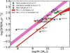 |
Fig. 1. SFR vs. stellar mass of our full galaxy sample. Sources at 5.5 < z < 7.5 with new and archival C III] data, galaxies at z ∼ 2 with archival C III] data, and literature sample at 6.0 < z < 7.5 are shown as blue, green, and orange circles, respectively. The best-fit relations for the main sequence (MS) at 5.5 < z < 7.5 and 1.7 < z < 2.0 from Schreiber et al. (2015) are shown as magenta and red bands, respectively. SFR and stellar mass references: HZ1, HZ10 – Capak et al. (2015); RXJ 1347−1216 – Huang et al. (2016), Bradač et al. (2017); GDS3073 – Grazian et al. (2020); UVISTA-Z-002 – Bowler et al. (2017a), Bouwens et al. (2022); COS-3018 – Smit et al. (2018); A383-5.2 – Matthee et al. (2019), Stark et al. (2015); z7_GND_42912 – Schaerer et al. (2015); Himiko – Carniani et al. (2018b), Graziani et al. (2020); CR7, CR7a, CR7b, CR7c – Matthee et al. (2017a); Bowler et al. (2014, 2017b); COS-13679 – Matthee et al. (2019), Laporte et al. (2017); COS-2987 – Smit et al. (2018), Laporte et al. (2017); VR7 – Matthee et al. (2019, 2017b); 9347, 6515, 10076, 9834, 9681, 8490 – this work, Zanella et al. (2018). |
Overview of the full galaxy sample used in this paper, grouped by C III] and [C II] detection.
3.1. New VLT/X-shooter observations
We opted for deep X-shooter observations with the purpose of investigating the C III] emission at λ1909 Å in three star-forming galaxies at z > 5, having [C II] detection at the location of the rest-frame FIR emission (Carniani et al. 2018a). The three targets are scattered by about 1.5 dex around the local L[C II] − SFR relation, thus allowing us to probe the C III] luminosity over a wide range of properties: 3 M⊙ yr−1 ≲ SFR ≲ 100 M⊙ yr−1, 107 L⊙ ≲ L[C II] ≲ 2.5 × 10⁹ L⊙, and −4 ≲ log(U) ≲ −1.5. Additionally, the availability of multi-bands observations (HST, Spitzer, and ALMA) for these targets enabled us to correct the C III] luminosity measurements from slit-losses (taking into account the size of the galaxy, the slit width, and the seeing) and dust extinction.
In particular, HZ1 and HZ10 have been observed with ALMA in [C II] by Capak et al. (2015), as part of their sample of normal star-forming galaxies at 5 < z < 6. Furthermore, the ALMA data has been reanalyzed by Carniani et al. (2018a), with a focus on a detailed morphological analysis of the [C II] emission. Specifically, for HZ10, the [C II] line reveals multiple components and the velocity gradient implies a merger scenario. Carniani et al. (2018a) measured [C II] luminosity of L[C II] = 2.5 ± 0.5 × 10⁸ L⊙ and L[C II] = 25.1 ± 5.0 × 10⁸ L⊙ for HZ1 and HZ10, respectively. Capak et al. (2015) found the total SFR of HZ1 and HZ10 of  and
and  , respectively. Our third target, RXJ 1347−1216 is a Lyα-emitting (LAE) galaxy at z ∼ 6.77 lensed by the RXJ 1347.1−1145 cluster (Huang et al. 2016). Bradač et al. (2017) detected the [C II] line emission with ALMA and measured a luminosity of
 ![$ L_{[{\mathrm{C}\,\textsc{II}}]} = 1.5_{-0.4}^{+0.2} \times 10^7\,L_{\odot} $](/articles/aa/full_html/2022/07/aa43336-22/aa43336-22-eq11.gif) , and estimated a SFR = 3.2 ± 0.4 M⊙ yr−. These authors found that the galaxy lies below the local [C II]–SFR relation (De Looze et al. 2014), in agreement with the expectations from the Vallini et al. (2015) model for a low-metallicity galaxy at z ∼ 7.
, and estimated a SFR = 3.2 ± 0.4 M⊙ yr−. These authors found that the galaxy lies below the local [C II]–SFR relation (De Looze et al. 2014), in agreement with the expectations from the Vallini et al. (2015) model for a low-metallicity galaxy at z ∼ 7.
We observed our targets with the VLT/X-shooter medium-resolution spectrograph (Vernet et al. 2011) on 02 April 2019, 19 April 2019, and 20 May 2019, respectively (European Southern Observatory (ESO) program ID: 0103.A-0692(A); PI: S. Carniani). The data for HZ1 and HZ10 were obtained over three observing blocks (OBs) of one hour each for every one of the three spectroscopic arms (UV/Blue (UVB), VISible (VIS), and Near-InfraRed (NIR)), in NODDING mode. An additional OB for each arm in STARE mode was carried out for each target, but it was not used in this work. For RXJ 1347−1216 source, only 1 OB was successfully obtained in NODDING mode for the VIS and NIR arms. The seeing variations were 0.31″ − 0.79″ and 0.34″ − 0.86″ for all OBs in the VIS and NIR arms, respectively. Sources were observed under clear conditions. All OBs used a 1.2″ slit with a resolution of R = 6500 and R = 4300 for the VIS and NIR arms, respectively.
3.2. Literature and archive sample
We included 11 sources at 6.0 < z < 7.5 with C III] and [C II] emission from the literature (see Table 1 for references) to build a large sample of high-z galaxies for our analysis. Out of these 11 systems, detection of both C III] and [C II] have been reported in two sources: COS-3018555981 (COS-3018 hereafter; Laporte et al. 2017; Smit et al. 2018) and A383-5.2 i.e., A383-5.1 (A383-5.2 hereafter2; Stark et al. 2015; Knudsen et al. 2016).
We also included GDS3073 and UVISTA-Z-002 with available X-shooter archival data of the C III] line and the [C II] line data either published in the literature (for GDS3073; Béthermin et al. 2020) or available in the ALMA archive (for UVISTA-Z-002; Bouwens et al. 2022). GDS3073 is a compact (r ≈ 0.11 kpc; Vanzella et al. 2010), active galactic nuclei (AGN) host galaxy at z ∼ 5.56, with a possible ongoing merger (Grazian et al. 2020) that has been detected in [C II] by ALMA (labeled as CANDELS_GOODSS_14; Béthermin et al. (2020) as part of the ALPINE survey (ALMA Large Program to INvestigate C+ at Early times; Le Fèvre et al. 2020). We retrieved and re-reduced (Sect. 4.2) the X-shooter archival data for GDS3073 from two ESO programs: 384.A-0886 (PI: A. Raiter) and 089.A-0679 (PI: N. Norgaard), previously presented by Grazian et al. (2020). UVISTA-Z-002 galaxy at z ∼ 6.75 was observed as a part of the REBELS (reionization-era bright emission line survey) ALMA large survey of z > 6.5 luminous star-forming galaxies (Bouwens et al. 2022). We retrieved and re-reduced (Sect. 4.2) the X-shooter archival data for UVISTA-Z-002 (ESO Program ID: 097.A-0082(A); PI: R. Bowler). For this source, we also used the [C II] observations from the ALMA archive in band 6 during Cycle 7 (Program ID: 2019.1.01634.L; PI: R. Bouwens).
Finally, we analyzed the VLT/MUSE (MultiUnit Spectroscopic Explorer) archival data (Program IDs: 094.A-0289(B), 095.A-0010(A), 096.A-0045(A), 099.A-0060(A), 098.A-0017(A), 096.A-0090(A), 0100.D-0807(C), 095.A-0240(A)) for a subsample of six galaxies at 1.75 < z < 1.95 for which [C II] detections were reported in Zanella et al. (2018).
4. Data reduction
4.1. Data reduction of the new VLT/X-shooter observations
We adopted the X-shooter pipeline (Modigliani et al. 2010) in the REFLEX (REcipe FLexible EXecution) environment3 to reduce the raw data. We also developed a Python script for the data analysis on the ESO pipeline final data products. We stacked the individual 2D spectra extracted from the OBs of each target, excluding bad pixels, and obtained a final weighted mean 2D spectra for the VIS and NIR spectra separately, by using the Drizzle package4. Next, we cropped the output 2D spectra at the wavelength range and slit position where we expect to see the Lyα and C III] lines in the VIS and NIR spectra, respectively. In order to increase the signal-to-noise ratio (S/N) of the emission lines, we also performed different spectral rebinning, depending on the expected width of the lines. Stacked, rebinned, and smoothed X-shooter 2D NIR spectra, and the extracted 1D spectra for HZ10, HZ1, and RXJ 1347−1216 are shown in Figs. 2, A.1, and A.2, respectively.
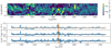 |
Fig. 2. X-shooter NIR spectrum of the HZ10 galaxy. Top panel: combined, rebinned (≈ 85 km s−1), and smoothed (1.1 nm × 0.12″) 2D spectrum. The C III] λλ1907, 1909 line is detected in the center of the slit with the negative flux on each side. The bottom three panels illustrate the extracted 1D spectra rebinned by ≈ 210 km s−1, ≈ 170 km s−1, and ≈ 140 km s−1, respectively. Shaded blue regions indicate the flux, dotted lines indicate the uncertainties, whereas orange solid line is the best Gaussian fit. Expected positions of the [C III] λ1907 at λ = 1269.7 nm and [C III] λ1909 line at λ = 1271.0 nm, based on the Lyα spectroscopic redshift, are shown as yellow and red lines, respectively. |
4.2. Reduction of the archival data
The retrieved X-shooter data of GDS3073 contains 21 OBs, of which 11 OBs from the program ID 384.A-0886 and 10 OBs from the program ID: 089.A-0679, for each arm. The NIR observations of the two programs are obtained in the different wavelength range. Therefore, we first stacked the individual 2D NIR spectra of each program separately, then we cropped the two 2D NIR spectra to be in the same wavelength range. We obtained the final 2D NIR spectrum as the weighted mean of the two 2D NIR spectra of each program. In order to extract the final 1D spectra, we followed the same procedure as described in Sect. 4.1. The results are shown in Fig. A.3.
The X-shooter archival data of UVISTA-Z-002 were retrieved with four OBs, for each of the three arms (ESO Program ID: 097.A-0082(A); PI: R. Bowler). For the data reduction step, we repeated the steps as in Sect. 4.1. The results are shown in Fig. A.4. For this source, we also reduced ALMA observations of the [C II] line by using CASA (common astronomy software applications) software5 (McMullin et al. 2007) and running the Python script delivered with the observations.
Finally, we used the VLT/MUSE archival data for a subsample of 1.75 < z < 1.95 galaxies for which [C II] line detection has been reported in Zanella et al. (2018). We extracted the 1D spectra from a circular region with a radius of r = 5″, enclosing the position of the target galaxy, and we analyzed the results using ds9 software6 and a Python script we developed. However, we still did not detect any C III] line emission in the extracted 1D spectrum of any source or in the stacked 1D spectrum of all the six galaxies from the MUSE subsample (see Fig. A.5).
5. X-shooter data analysis: C III] line emission
We visually inspected the X-shooter VIS and NIR 1D spectra for the Lyα, C III], and any additional rest-frame UV emission line for each source. Next, we rebinned the 1D spectra to increase the signal-to-noise ratio and we fitted the line emission with a Gaussian to derive the integrated flux.
We recovered the Lyα emission detection in HZ1 and HZ10, previously reported in Capak et al. (2015) with the DEIMOS spectrograph on the Keck II telescope. We also identified a hint of the Lyα emission in RXJ 1347-1216, previously published in Huang et al. (2016) with DEIMOS. Next, in the NIR 2D spectrum and the extracted 1D spectra of the HZ10 galaxy, we identified the blended C III] λλ1907, 1909 doublet line at the expected redshifted wavelength position of the C III] line, at λ ≈ 1270 nm (Fig. 2, top panel). The feature with a positive flux is in the center of the slit with two negative flux features on each side of the positive emission (Fig. 2, top panel), as data were taken in the NODDING mode.
The X-shooter spectrograph allows us to resolve the C III] λλ1907, 1909 doublet. However, in order to detect the C III] with a statistically significant S/N, we need to rebind the spectra via 15 channels (≈ 200 km s−1), which decreases the spectral resolution. Therefore, we did not ultimately detect the two lines separately, so we fit the C III] doublet with a single Gaussian, from which we obtained a total integrated flux of 8.8 ± 2.1 × 10⁻¹⁷ erg s−1 cm−2 with a S/N = 4.2 and a FWHM = 550.9 ± 98.8 km s−1. The peak of the doublet line occurs at λ = 1269.4 ± 0.2 nm, which is slightly blueshifted than the expected positions of the [C III] λ1907 line at λ = 1269.7 nm and C III] λ1909 line at λ = 1271.0 nm, based on the Lyα spectroscopic redshift from Capak et al. (2015; Fig. 2, yellow and red vertical lines, respectively). However, at high-z, a significant part of the Lyα emission can be absorbed by the increasing fraction of the neutral medium and the peak of the observed Lyα emission might be offset with respect to the systematic redshift (Dijkstra 2014). If we take the spectroscopic redshift based on the [C II] line emission from Capak et al. (2015), the expected positions of the two C III] lines are at λ = 1269.2 nm and λ = 1270.5 nm, and the peak of the doublet line occurs between the two separate lines.
Assuming a [C III] λ1907/C III] λ1909 line ratio of 1.4 ± 0.2 (Stark et al. 2015), we estimated the C III] λ1909 line integrated flux of 3.7 ± 1.1 × 10⁻¹⁷ erg s−1 cm−2 with S/N = 3.4. For the other two targets, HZ1 and RXJ 1347−1216, we did not detect C III] emission at the expected redshifted wavelength and we place a 3σ upper limit on the line flux. For HZ1 and RXJ 1347−1216, we estimate the integrated flux upper limit assuming a full-width at half maximum (FWHM) of the C III] line to be equal to the FWHM of the [C II] line, where FWHM[C II] = 72 ± 11 km s−1 (Capak et al. 2015) and FWHM[C II] = 75 ± 25 km s−1 (Bradač et al. 2017), respectively. Furthermore, we inspected the VIS and NIR spectra of our targets, but we did not detect any additional UV-rest frame lines.
GDS3073 has been observed with FORS2, VIMOS, and X-shooter spectrographs at the VLT telescope and several UV rest-frame line detection have been reported, including N V] λ1240 and O VI λ1032 − 1038, confirming the AGN nature of GDS3073 (Vanzella et al. 2010; Grazian et al. 2020). We recover a very bright Lyα emission detection with a S/N ∼ 22 and NIV] line emission with a S/N ∼ 3.9. For the C III] line, we place an upper limit on the velocity integrated flux, assuming FWHM[C III] = FWHM[C II], where the FWHM[C II] = 230 ± 16 km s−1 derived by Béthermin et al. (2020). In the spectra of UVISTA-Z-002, we did not detect any emission line. We placed a 3σ upper limit on the C III] line flux and estimated the velocity integrated flux upper limit, assuming FWHM[C III] = FWHM[C II], where FWHM[C II] = 45.2 ± 7.6 km s−1 was obtained from the Gaussian fit on the observed [C II] line from this work.
For the intermediate-z galaxy sample, we did not identify any emission at the expected location of the C III] line in the extracted 1D spectra of each individual galaxy nor in the stacked spectrum. Therefore, we set an upper limit to the C III] flux and we estimated the velocity integrated flux assuming FWHM[C III] = FWHM[C II], with the FWHM of the [C II] line estimates from Zanella et al. (2018). The observed C III] line flux of the entire sample of galaxies is in Table 2.
UV radius, observed and intrinsic C III] line emission flux, C III] intrinsic luminosity, and surface brightness of the full galaxy sample.
6. Results
In the previous section, we derived the C III] λ1909 line integrated flux of ![$ F_{{\mathrm{C}\,\textsc{III}}]}^\mathrm{{obs}} = \rm{3.7 \pm 1.1 \times 10^{-17}\,erg\,s^{-1}\,cm^{-2}} $](/articles/aa/full_html/2022/07/aa43336-22/aa43336-22-eq18.gif) for HZ10. We also included a literature sample of three z > 6 galaxies: COS-3018 (Laporte et al. 2017; Smit et al. 2018), A383-5.2 (Stark et al. 2015; Knudsen et al. 2016), and z7_GND_42912 (Hutchison et al. 2019; Schaerer et al. 2015), with the observed C III] integrated flux in the range of
for HZ10. We also included a literature sample of three z > 6 galaxies: COS-3018 (Laporte et al. 2017; Smit et al. 2018), A383-5.2 (Stark et al. 2015; Knudsen et al. 2016), and z7_GND_42912 (Hutchison et al. 2019; Schaerer et al. 2015), with the observed C III] integrated flux in the range of ![$ F_{{\mathrm{C}\,\textsc{III}}]}^\mathrm{{obs}} = \rm{1.3{-}3.7 \times 10^{-18}\,erg\,s^{-1}\,cm^{-2}} $](/articles/aa/full_html/2022/07/aa43336-22/aa43336-22-eq19.gif) .
.
As a rest-frame UV line at λ = 1909 Å, the C III] is expected to be affected by dust attenuation (see, e.g., Salim & Narayanan 2020 and references therein). Therefore, we correct the C III] emission for the dust attenuation and derive the attenuation-corrected C III] integrated flux for galaxies with C III] detection, whereas for non-detections, we did not perform this correction. Next, we constrained the burstiness parameter, κs, metallicity, Z, and the total density of the emitting gas, n, with the use of the Vallini et al. (2020) model. Finally, we compare the ISM properties of HZ10 and COS-3018 derived in this work and in the literature.
6.1. Intrinsic C III] line emission
We derived the UV attenuation at 1900 Å, following Meurer et al. (1999):
where βUV is the UV-continuum slope (fλ ∝ λβUV; Calzetti et al. 1994) of sources with C III] detection from the literature (Table 3), dAUV/dβUV is the steepness of the dust attenuation law and βUV, intr is the intrinsic UV-continuum slope. Meurer et al. (1999) has derived this correlation to estimate the UV attenuation at 1600 Å. However, we use the same correlation to derive the UV attenuation at 1900 Å, assuming that the attenuation is nearly identical at two wavelengths. Next, to make use of Eq. (6), we need to determine the dAUV/dβUV and βUV, intr parameters, which depend on the dust attenuation curve of a galaxy. In order to constrain the dust attenuation law, we can use the IRX − βUV diagram, where IRX is the infrared excess parameter IRX = LFIR/LUV. HZ10 is a massive, metal-rich, star-forming galaxy (Capak et al. 2015; Faisst et al. 2017) that falls on the local starburst relation (Barisic et al. 2017; Faisst et al. 2017), with dAUV/dβUV = 1.99 and βUV, intr = −2.23 (Meurer et al. 1999). However, for the remaining three sources: COS-3018, A383-5.2 and z7_GND_42912, only upper limits on the LFIR and, thus, the IRX parameter, are reported in the literature, which also depends on the assumption on the dust temperature (Behrens et al. 2018; Sommovigo et al. 2020, 2022). Therefore, it is not possible to constrain the dust attenuation curve of these objects, since they could fall on any of the many variants of the dust attenuation law (e.g., Meurer et al. 1999). Therefore, for these z > 5 sources, we estimated the UV attenuation, A1900, assuming that they lie on the fiducial relation for local starbursts, in agreement with results for high-z galaxies from the literature (Fudamoto et al. 2020; Vijayan et al. 2021). Values of the derived UV attenuation A1900 are given in Table 3.
βUV slope and UV attenuation at 1900 Å for three z > 5 galaxies with C III] and [C II] detections.
The absorption law slope for local starbursts found by Meurer et al. (1999) is consistent with the Calzetti dust attenuation law (Calzetti et al. 2000). Thus, the intrinsic C III] flux of high-z sources can be derived from the observed C III] flux using the Calzetti attenuation law as:
![$$ \begin{aligned} F_{\rm {{{\text{C}}{\small {{\text{ III}}}}]}}}^\mathrm{{int}} = F_{\rm {{{\text{C}}{\small {{\text{ III}}}}]}}}^\mathrm{{obs}} \ 10^{0.4 A_{1900}}. \end{aligned} $$](/articles/aa/full_html/2022/07/aa43336-22/aa43336-22-eq22.gif)
For HZ10, we derived the intrinsic flux of the C III] line of 6.5 ± 2.0 × 10⁻¹⁷ erg s−1 cm−2, which is higher than the observed value by a factor of ≈1.8.
We derived the intrinsic surface brightness of the C III] line as:
![$$ \begin{aligned} \Sigma _{{\text{C}}{\small {{\text{ III}}}}]}^\mathrm{{int}} = \frac{L_{{\text{C}}{\small {{\text{ III}}}}]}^\mathrm{{int}}}{2 \pi r_{\rm {UV}}^2}, \end{aligned} $$](/articles/aa/full_html/2022/07/aa43336-22/aa43336-22-eq23.gif)
where rUV is the UV radius in kpc tracing the C III] emitting ionized phase of the ISM, ![$ L_{{\mathrm{C}\,\textsc{III}}]}^\mathrm{{int}} = 4 \pi D_{\mathrm{L}}^2 F_{{\mathrm{C}\,\textsc{III}}]} $](/articles/aa/full_html/2022/07/aa43336-22/aa43336-22-eq24.gif) is the intrinsic luminosity in solar luminosity L⊙ and DL is the luminosity distance in Mpc. For the z7_GND_42912 source, we derive the UV radius rUV using the Hubble Space Telescope (HST) Wide-Field Camera 3 (WFC3) image of the galaxy in the F160W filter, as well as the QFitsView7 and Aladin8 astronomical tools. We fit the image of the galaxy with an elliptical Gaussian and measure the FWHM in pixels. Next, we derived the FWHM in ″, deconvolved by the FWHM of the point-spread function (PSF) for the (HST) WFC3 camera of FWHMPSF = 0.18 ± 0.01 arcsec (e.g., Law et al. 2012). Finally, we derived the deconvolved UV radius in kpc. For most of the galaxies included in our analysis, we use rUV from the literature. For UVISTA-Z-002, COS-3018, and COS-2987, rUV is not measured in the literature, so we assume rUV ∼ 0.5 r[C II], following Carniani et al. (2018a). For six intermediate-z galaxies, we estimate the UV radii rUV using the HST Advanced Camera for Surveys (ACS) images in the b magnitude, with a FWHMPSF = 0.08 arcsec (e.g., Windhorst et al. 2011) and following the above-mentioned procedure. The spectroscopic redshift, UV radius, observed, and intrinsic C III] line emission flux, C III] intrinsic luminosity and C III] intrinsic surface brightness of the entire galaxy sample used in this work are given in Table 2.
is the intrinsic luminosity in solar luminosity L⊙ and DL is the luminosity distance in Mpc. For the z7_GND_42912 source, we derive the UV radius rUV using the Hubble Space Telescope (HST) Wide-Field Camera 3 (WFC3) image of the galaxy in the F160W filter, as well as the QFitsView7 and Aladin8 astronomical tools. We fit the image of the galaxy with an elliptical Gaussian and measure the FWHM in pixels. Next, we derived the FWHM in ″, deconvolved by the FWHM of the point-spread function (PSF) for the (HST) WFC3 camera of FWHMPSF = 0.18 ± 0.01 arcsec (e.g., Law et al. 2012). Finally, we derived the deconvolved UV radius in kpc. For most of the galaxies included in our analysis, we use rUV from the literature. For UVISTA-Z-002, COS-3018, and COS-2987, rUV is not measured in the literature, so we assume rUV ∼ 0.5 r[C II], following Carniani et al. (2018a). For six intermediate-z galaxies, we estimate the UV radii rUV using the HST Advanced Camera for Surveys (ACS) images in the b magnitude, with a FWHMPSF = 0.08 arcsec (e.g., Windhorst et al. 2011) and following the above-mentioned procedure. The spectroscopic redshift, UV radius, observed, and intrinsic C III] line emission flux, C III] intrinsic luminosity and C III] intrinsic surface brightness of the entire galaxy sample used in this work are given in Table 2.
6.2. [C II] line emission and SFR
For UVISTA-Z-002, we fit the observed [C II] line emission with a Gaussian from which we derived an integrated flux of 35.5 ± 7.7 mJy beam−1 km s−1, with a S/N = 4.5 and a FWHM = 45.2 ± 7.6 km s−1. Peak of the Gaussian is at 1204.1 μm, corresponding to a spectroscopic redshift of zsp = 6.634 ± 0.004 which is consistent with the previous measurement of the photometric redshift zph = 6.75, with uncertainties in the range of Δzph = 0.07 − 0.09 (Bouwens et al. 2022). Next, we derived the [C II] surface brightness Σ[C II] as:
![$$ \begin{aligned} \Sigma _{[{\text{C}}{\small {{\text{ II}}}}]} = \frac{L_{ [{\text{C}}{\small {{\text{ II}}}}]}}{2 \pi r_{\rm {[{\text{C}}{\small {{\text{ II}}}}]}}^2}, \end{aligned} $$](/articles/aa/full_html/2022/07/aa43336-22/aa43336-22-eq25.gif)
where ![$ L_{ [{\mathrm{C}\,\textsc{II}}]} = 1.04 \times 10^{-3} S_{ [{\mathrm{C}\,\textsc{II}}]} \Delta {v} D_{\mathrm{L}}^2 $](/articles/aa/full_html/2022/07/aa43336-22/aa43336-22-eq26.gif) is [C II] luminosity in units of solar luminosity from Carilli & Walter (2013), S[C II] Δv is the velocity integrated flux of the [C II] line, DL is the luminosity distance in Mpc, vobs is the observed frequency in GHz, and r[C II] is the [C II] radius in kpc. For UVISTA-Z-002, we measure r[C II] from the ALMA continuum-subtracted, [C II] line map, and the imfit task of the CASA software (version-6.4.0-16). We fit the [C II] emitting region of the source with an elliptical Gaussian and measure the beam-deconvolved FWHM in ″, from which we derived the r[C II] in kpc. For the other sources from our sample, we used the r[C II] values from the literature when available or we assume r[C II] following Carniani et al. (2018a).
is [C II] luminosity in units of solar luminosity from Carilli & Walter (2013), S[C II] Δv is the velocity integrated flux of the [C II] line, DL is the luminosity distance in Mpc, vobs is the observed frequency in GHz, and r[C II] is the [C II] radius in kpc. For UVISTA-Z-002, we measure r[C II] from the ALMA continuum-subtracted, [C II] line map, and the imfit task of the CASA software (version-6.4.0-16). We fit the [C II] emitting region of the source with an elliptical Gaussian and measure the beam-deconvolved FWHM in ″, from which we derived the r[C II] in kpc. For the other sources from our sample, we used the r[C II] values from the literature when available or we assume r[C II] following Carniani et al. (2018a).
To constrain the ISM parameters with the Vallini et al. (2020) method, we also included the total SFR per unit area, which is derived as:
where SFR = SFRUV + SFRIR is the total SFR and rUV is the UV radius tracing the extension of the star-forming regions (Carniani et al. 2018a). We either make use of the SFRUV and SFRIR given in the literature, converted to the Kennicutt & Evans (2012) scaling relations, when necessary; or we constrain these parameters using the corresponding UV and IR luminosities, along with the scaling relations of Kennicutt & Evans (2012). For GDS3073 and the z ∼ 2 sources of our sample, the UV luminosity LUV is not reported in the literature. Therefore, for these objects we computed the LUV from the absolute magnitudes corresponding to rest-frame UV (Graziani et al. 2020). Moreover, for some high-z galaxies no SFRIR estimates or only upper limits are provided in the literature. For those sources, we assumed SFR = SFRUV. Table 4 shows the [C II] radius, luminosity and surface brightness, and total SFR and SFR per unit area for the full galaxy sample. Figure 3 shows [C II] surface brightness vs. C III] surface brightness, color-coded with the SFR per unit area, for our entire sample of galaxies. We observe that galaxies with high C III] and [C II] surface brightness tend to experience high SFR per unit area, although the data are scattered and most of the sources have only C III] upper limits.
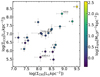 |
Fig. 3. [C II] surface brightness Σ[C II] vs. C III] surface brightness Σ[[C III], color-coded by the SFR per unit area ΣSFR, for our entire sample of galaxies. Sources that are detected both in [C II] and C III] are annotated. |
[C II] radius, luminosity and surface density, and total SFR, and SFR per unit area of the full galaxy sample.
6.3. ISM parameters: κs, Z, and n
In this section we exploit the C III] and [C II] emission to constrain the ISM properties of the selected sample. By adopting the model by Vallini et al. (2020), which depends on Σ[[C III], Σ[C II] and ΣSFR, we can determine the total gas density n, gas-phase metallicity Z, and the deviation from the KS relation, quantified by the burstiness parameter κs.
We initially applied the Vallini et al. (2020) model on those galaxies that are detected both in C III] and [C II] emission. The results are reported in Table 5. For the other sources with upper limits on either the C III] or [C II] emission, we constrained the ISM parameters, assuming that the upper limits are measured values with uncertainties equal to 25% of the upper limit estimates. We report the derived values for these sources in Table C.1 (Appendix C). The detected high-z galaxies have a gas-phase metallicity in the range 0.2 Z⊙ ≲ Z ≲ 0.6 Z⊙ and a total gas density in the range 2.4 ≲ log(n[cm−3]) ≲ 3.4. On average, all galaxies deviate from the KS relation by about one order of magnitude (1.1 ≲ log(κs) ≲ 1.4). This implies that these early galaxies are mostly in a starburst phase, with a higher star formation rate with respect to their gas content. Furthermore, the available data at 5 < z < 7 suggest that the KS relation is not universal and it might be shifted upwards at higher redshift (Vallini et al. 2021; Pallottini et al. 2022; see Carilli & Walter 2013 and Krumholz 2015 for reviews).
Burstiness parameter κs, gas metallicity Z, and gas density n for the three z > 5 galaxies detected in both C III] and [C II].
We note that Pavesi et al. (2019) derived a lower κs parameter log(κs) ≈ −1 for HZ10, by observing the CO(2-1) line, which implies a low star formation efficiency for this source. The conflict between the two results can be explained by the fact that Pavesi et al. (2019) estimated the gas mass by adopting a large CO-to-Mgas conversion factor αCO = 4.5 M⊙ (K km s−1 pc2)−1, a value that is close to the Galactic conversion factor αCO = 4.36 M⊙ (K km s−1 pc2)−1 (Bolatto et al. 2013). Although the Galactic conversion factor is a derived value for Milky Way and normal, star-forming galaxies in the local Universe, it may not be applicable for more extreme environments of starburst galaxies at high-z (see Carilli & Walter 2013 for a review). The conversion factor depends on the physical conditions of the gas in the ISM (temperature, surface density, dynamics, and metallicity), as well as the star formation and associated feedback (Narayanan et al. 2011, 2012; Genzel et al. 2012; Feldmann et al. 2012; Renaud et al. 2019; see, e.g., Bolatto et al. 2013 for a review). It is typically in the range between 0.8 and 4.36 M⊙ (K km s−1 pc2)−1 (see, e.g., Bolatto et al. 2013; Carilli & Walter 2013, and Combes 2018 for reviews). Low metallicities (Z = 0.6 Z⊙ for HZ10) will drive αCO towards values higher than the Galactic value (Narayanan et al. 2012; Genzel et al. 2012; Popping et al. 2014), although αCO spans a broad range of values of αCO ∼ 0.4 − 11 M⊙ (K km s−1 pc2)−1, due to large uncertainties (see, e.g., Fig. 9 of Bolatto et al. 2013). On the other hand, high values of temperature, surface density, and velocity dispersion in a turbulent ISM of starbursts and merging systems will shift αCO towards lower values (Narayanan et al. 2011, 2012; Vallini et al. 2018). HZ10 has an extremely high value of the burstiness parameter log(κs) ∼ 1.4 and high total density of the [C II] emitting gas log(n) ∼ 3.35 cm−3, and it is also a multi-component system (Jones et al. 2017, Carniani et al. 2018a). Thus, for this source we assumed αCO = 0.8 M⊙ (K km s−1 pc2)−1, usually adopted for starburst galaxies (e.g., Downes & Solomon 1998; Bolatto et al. 2013). We obtained log(κs) = 0.53 ± 0.34, which is within the 2σ uncertainties of the  , estimated exploiting the C III] emission and the Vallini et al. (2020) model.
Finally, we also note that the best-fit results estimated for COS-3018 are different from those reported by Vallini et al. (2020), even though both works are based on the same model and the C III] and [C II] emission. Vallini et al. (2020) found that COS-3018 is a moderate starburst with log(κs) ≈ 0.5, with a mean gas density log(n[cm−3]) ≈ 2.7 and a gas metallicity of Z ≈ 0.4 Z⊙. The derived ISM properties are consistent with our values, apart from the burstiness parameter, which is log(κs) ≈ 1.1. The high value of the κs parameter derived in our work is mainly driven by the value of the intrinsic C III] flux which is by a factor of ∼6.5 higher, namely, FC III] ≈ 8.5 × 10⁻¹⁸ erg s−1 cm−2. On the other hand, Vallini et al. (2020) used a lower value of the observed C III] flux of FC III] ≈ 1.3 × 10⁻¹⁸ erg s−1 cm−2 (Laporte et al. 2017), without considering the correction for the dust attenuation.
7. Discussion
In this section, we analyze the distribution of high-z galaxies in the Σ[C II] − ΣSFR space and compare it with the local relation from De Looze et al. (2014) and recent theoretical models. Next, we investigate the possible correlation between the ISM properties: κs, Z, and n, as well as the deviation from the local relation, namely, the Δ parameter.
7.1. Σ[C II] − ΣSFR relation
De Looze et al. (2014) found a tight relation between the [C II] emission and SFR for a sample of spatially resolved, low-metallicity dwarf galaxies in the local Universe, which can be expressed as:
![$$ \begin{aligned} \mathrm {\log {(\Sigma _{SFR})}} = -6.99 + 0.93\ \mathrm {\log {(\Sigma _{[{\text{C}}{\small {{\text{ II}}}}]})}}. \end{aligned} $$](/articles/aa/full_html/2022/07/aa43336-22/aa43336-22-eq46.gif)
We investigate whether this relation is still valid in the high-z Universe. In Fig. 4, we show the [C II] surface brightness and SFR per unit area of our entire sample of high-z (5.5 < z < 7.5) and intermediate-z (z ∼ 2) galaxies. To increase our sample and cover a broader range of redshift as well as the Σ[C II] − ΣSFR parameter space, we also include a subsample of 38 galaxies from the ALPINE survey at 4 < z < 6, for which [C II] measurements and radii are well constrained and available in the literature (Le Fèvre et al. 2020; Fujimoto et al. 2020; Béthermin et al. 2020) and we derived their total SFR from the UV and IR luminosities (if the galaxies are detected in the IR).
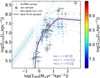 |
Fig. 4. [C II] surface brightness vs. SFR per unit area, color-coded by the C III] surface brightness, of this sample of galaxies. Filled and empty circles indicate sources with the C III] line detection and upper limits, respectively. Galaxies detected both in [C II] and C III] emission are annotated. Blue × symbols indicate a subsample of galaxies from the ALPINE survey at 4 < z < 6 (Le Fèvre et al. 2020). Σ[C II] − ΣSFR relation for local galaxies by De Looze et al. (2014) is represented as a blue dashed line with a 1σ dispersion of 0.32 dex. This relation is extrapolated to cover the distribution of high-z sources in Σ[C II] − ΣSFR space, which is shown as a light-blue dashed line. Σ[C II] − ΣSFR relation predictions from models of Ferrara et al. (2019) with three different combinations of fixed κs, Z, and n parameters (Table 5) are represented as dotted gray lines. Finally, the best-fit model (Z = 0.24 Z⊙, log(n[cm−3]) = 2.98, and log(κs) ≈ 1.30) on all the galaxies (excluding Z7_GND_42912) and 100 random samples from the MCMC chain are shown as thick and thin purple solid lines, respectively. |
All of the sources lie below the Σ[C II] − ΣSFR local relation by De Looze et al. 2014 (Fig. 4, blue dashed line). This is consistent with the results of Carniani et al. (2018a) in a sample of z > 5 star-forming galaxies. We note that part of the De Looze et al. (2014) local relation in Fig. 4 is an extrapolation of the actual relation found by De Looze et al. (2014), since their sample of spatially resolved dwarf galaxies covers a lower range of values in the Σ[C II] − ΣSFR space, with 4.5 ≲ log((Σ[C II])[L⊙ kpc−2]) ≲ 7.0 and −3 ≲ log(ΣSFR[M⊙ yr−1]) ≲ 0, compared to most high-z sources used in this work.
In Fig. 4, we report three Σ[C II] − ΣSFR models by Ferrara et al. (2019) that fit the three high-z sources with both C III] and [C II] detections (dotted gray lines), for which the ISM properties are constrained in Sect. 6.3 (Table 5). We can notice that the model with fixed ISM properties of the HZ10 source (log(κs) ≈ 1.43, Z = 0.6 Z⊙, and log(n[cm−3]) = 3.35), passes through HZ10 and A383-5.2. However, this model overestimates the κs parameter in A383-5.2, because κs is mainly driven by very high C III] emission, which is not observed in A383-5.2. Therefore, the model with fixed ISM properties of the A383-5.2 source (log(κs) ≈ 1.13, Z = 0.24 Z⊙, and log(n[cm−3]) = 2.41) is clearly a better fit for the A383-5.2 galaxy.
Next, we show the best-fit model of our full sample (excluding Z7_GND_42912 as it is not detected in [C II]) and the ALPINE subsample (Fig. 4, solid purple line). The best-fit model for these high-z sources points to reasonable average values of subsolar metallicity Z = 0.24 Z⊙, high density log(n[cm−3]) = 2.98, and a very high burstiness parameter log(κs) ≈ 1.3 with respect to the local dwarf sample from De Looze et al. (2014). The high mean value of the κs parameter is another strong piece of evidence in favor of the KS relation being shifted upwards at higher-z (Vallini et al. 2021; Pallottini et al. 2022). We will discuss this aspect in more detail in an upcoming work.
Overall, these models show that the [C II] faintness of high-z star-forming galaxies might be driven by a combination of high burstiness parameter, low metallicity, and total gas density. Clearly, it would be possible to fit a single source with multiple models since there is a degeneracy between the ISM parameters: Z, n, and κs. Therefore, besides the [C II] line data, observations of an additional line tracing the ISM is necessary to resolve the degeneracy between these three parameters.
In Fig. 5, we show the deviation from the local Σ[C II] − ΣSFR relation Δ and the C III] over [C II] surface brightness ratio, color-coded by the total SFR per unit area ΣSFR. The Δ parameter is generally decreasing, namely, |Δ| is increasing, with the increase of the ΣC III]/Σ[C II] ratio and ΣSFR, as expected from the model of Vallini et al. (2020). We overplot the grid of model predictions with fixed Z and n, allowing for κs and ΣSFR to vary in a broad range of values of 0 ≤ log(κs) ≤ 2.4 (Fig. 5, dashed lines) and −0.5 ≤ log(ΣSFR[M⊙ yr−1]) ≤ 2.5 (Fig. 5, solid lines), respectively. In the top panel of Fig. 5, we show a model example with a solar metallicity Z = Z⊙ and total gas density of log(n[cm−3]) = 3.3, equivalent to the HZ10 example model shown in Fig. 4 (dashed purple line). Moreover, in the bottom panel of Fig. 5, we show an example with Z = 0.5 Z⊙ and log(n[cm−3]) = 2.5, typical values for high-z galaxies (Pallottini et al. 2017). We can observe that the first model correctly reproduces the ΣSFR parameters for the HZ10 source, whereas the second model reproduces ΣSFR correctly for most of the other galaxies from our sample (Fig. 5, top and bottom panel, respectively), implying that a subsolar metallicity is a more plausible average value for the large majority of high-z star-forming galaxies.
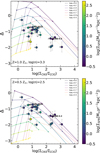 |
Fig. 5. Deviation from the local Σ[C II] − ΣSFR relation Δ vs. the C III] over [C II] surface brightness ratio, color-coded by the SFR per unit area ΣSFR. Galaxies detected both in [C II] and C III] emission are annotated. We plot a grid of model predictions with fixed metallicity and gas density, with the burstiness parameter varying in a range of 0 ≤ log(κs) ≤ 2.4 i.e., κs = 1, 5, 10, 30, 50, 100, 250 (dotted lines), and log(ΣSFR[M⊙ yr−1]) in −0.5 ≤ log(ΣSFR[M⊙ yr−1]) ≤ 2.5 (solid lines). The top panel shows an example of a model prediction for high-z galaxies with ISM properties similar to HZ10, with solar metallicity Z = Z⊙ and gas density close to critical density of log(n[cm−3]) = 3.3. Bottom panel shows predictions for typical high-z galaxies with subsolar metallicity Z = 0.5 Z⊙ and log(n[cm−3]) = 2.5. |
7.2. Correlation between the deviation and ISM properties
We now assess whether the [C II] deficit depends on the ISM properties. In particular, we investigate the relation between the Δ parameter and ISM properties, focusing mostly on the κs and n, because Z is not well constrained by the model.
Since, in our sample, we have only three galaxies for which κs and n are well constrained, in this part of our analysis, we include a sample of galaxies in the EoR (at 6 < z < 9) with κs, Z, and n constrained by Vallini et al. (2021). This method is equivalent to the Vallini et al. (2020) method9 used in this work, with the exception of a different line used as a ionized gas tracer, namely: the [O III] line at λ = 88 μm.
In Fig. 6, we report the burstiness parameter κs and the deviation from the Σ[C II] − ΣSFR relation Δ. Next, we explore the correlation between the κs and Δ by using the Spearmann rank correlation, resulting into a correlation coefficient of ρ ≈ −0.27 and the p-value of p = 0.35. Thus, current data seem to indicate that the [C II] deficit is anti-correlated to the burstiness parameter, but it is not statistically significant. From the best-fit on the detected z > 5 sources we see that κs is increasing with the decrease of the Δ parameter, that is, as galaxies undergo a larger deviation from the local De-Looze relation, |Δ| is increasing if they are in a more “bursty” phase (Fig. 6, blue line). This is expected, since intense radiation fields emitted by young massive stars in starburst galaxies with κs ≫ 1 are strong enough to photo-evaporate molecular clouds (Decataldo et al. 2019) and the PDRs bound to them, from where the bulk of the [C II] emission originates (Vallini et al. 2015, 2017). Consequently, strong UV radiation will alter the ionization state of the bulk of the gas, including carbon, which will emit more in C III] or higher ionization states (e.g., Ferrara et al. 2019; Vallini et al. 2020). Therefore, these starbursts are expected to deviate from the local Σ[C II] − ΣSFR relation.
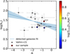 |
Fig. 6. Burstiness parameter κs vs. deviation from the local De-Looze relation Δ, color-coded by the C III] surface brightness ΣC III]. Galaxies detected both in [C II] and C III] emission are annotated and represented as filled circles. Galaxies at 6 < z < 9 from Vallini et al. (2021) are represented as gray stars. Linear fit on the detected sources is shown as a blue line with 1σ uncertainties as a shaded region. |
Figure 7 illustrates the total gas density n as a function of the deviation from the local De-Looze relation Δ for high-z galaxies. We derive the Spearmann correlation coefficient of ρ ≈ 0.86 and the p-value of p = 5.68 × 10⁻⁵. Thus, the total gas density, n, shows the strongest correlation with the Δ parameter out of any ISM property considered in this work. The best fit on the detection points shows that sources with low density, n, tend to experience a larger deviation from the local De-Looze relation. This agrees with the interpretation of Ferrara et al. (2019), who found that extremely diffuse high-z systems with n ≈ 20 cm−3 will have a low [C II] surface brightness (e.g., CR7c with Σ[C II] ∼ 106 L⊙kpc−2). This is primarily a consequence of the fact that the [C II] emitting region can be spatially more extended than their star-forming region (Carniani et al. 2018a; Fujimoto et al. 2019). The extended [C II] emission may originate from the outflowing [C II] emitting gas or the [C II] circumgalactic medium, whereas the star-forming region, traced by the rest-frame UV emission, may be heavily dust-obscured (Carniani et al. 2018a; Gallerani et al. 2018; Fujimoto et al. 2019). Furthermore, low density systems at high-z tend to experience more CMB suppression effects on the [C II] line emission (Kohandel et al. 2019). Finally, in low-density systems, FUV photons may be able to penetrate deeper into the ISM and ionize more of its gas, which will lead to carbon emitting less in [C II] and more in higher ionization states.
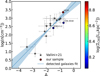 |
Fig. 7. Density of the emitting gas n vs. deviation from the local De-Looze relation Δ, color-coded by the C III] surface brightness Σ[[C III]. Symbols are the same as in Fig. 6. |
8. Summary and conclusions
In this work, we present an analysis of the novel VLT/X-shooter observations targeting the C III] line emission in three high-z galaxies: HZ1 at z ∼ 5.69, HZ10 at z ∼ 5.66, and RXJ 1347−1216 at z ∼ 6.77. We have included the archival X-shooter data of two other sources: GDS3073 at z ∼ 5.56 and UVISTA-Z-002 at z ∼ 6.63. We have also included the VLT/MUSE archival data of six galaxies at z ∼ 2. We have extended our sample of galaxies with 11 star-forming systems at 6.0 < z < 7.5 with C III] and [C II] detection or upper limits reported in the literature. We have combined the data on the C III] surface brightness Σ[[C III], [C II] surface brightness Σ[C II], and SFR per unit area ΣSFR with the model of Vallini et al. (2020), to characterize the ISM properties of high-z galaxies: the burstiness parameter, κs, metallicity, Z, and total gas density, n. Finally, we have investigated the correlation of the different ISM properties with the deviation from the local Σ[C II] − ΣSFR relation found by De Looze et al. (2014). Our main results are:
-
The X-shooter observations reveal a line emission associated with the blended C III] λλ1907, 1909 doublet line in the HZ10 source. We extracted the 1D spectrum and measured an integrated flux of the C III] λλ1907, 1909 line of 8.8 ± 2.1 × 10⁻¹⁷ erg s−1 cm−2. We derived the C III] λ1909 integrated flux of 3.7 ± 1.1 × 10⁻¹⁷ erg s−1 cm−2, assuming the [C III] λ1907/C III] λ1909 line ratio of 1.4 ± 0.2. For the other two targets: HZ1, RXJ 1347−1216, and other galaxies drawn from the archive, we placed 3σ upper limits on the C III] line flux (Table 2).
-
We correct the observed C III] line flux for the dust attenuation, using the Calzetti attenuation law (Calzetti et al. 2000), for HZ10 and a handful of other z > 6 galaxies: COS-3018, A383-5.2 and Z7_GND_42912, with C III] emission reported in the literature. For HZ10, we derived the intrinsic C III] line flux of 6.5 ± 2.0 × 10⁻¹⁷ erg s−1 cm−2.
-
We derived an integrated flux of 35.5 ± 7.7 mJy beam−1 km s−1 of the [C II] line emission for the UVISTA-Z-002 galaxy. For the other galaxies from our sample, we included the [C II] line luminosity from the literature. For our analysis, we also included the total SFR data, either from the literature or derived from the UV and IR luminosities (Table 4).
-
We characterized the burstiness parameter, κs, total gas density, n, and metallicity, Z, with the use of the C III] and [C II] emission and Vallini et al. (2020) model. High-z star-forming galaxies predominantly show subsolar metallicities. The majority of all the high-z sources are in the starburst phase with log(κs) ≳ 1, implying that the ΣSFR − Σgas relation is shifted upwards at early epochs.
-
We constrain the burstiness parameter
 for HZ10. This is not consistent with log(κs) ≈ −1, found by Pavesi et al. (2019). Using CO measurements of Pavesi et al. (2019) and assuming a lower conversion factor αCO = 0.8 M⊙ (K km s−1 pc2)−1, we obtain log(κs) = 0.53 ± 0.34. This value is approximately within the 2σ uncertainties of the log(κs) estimated using the C III] emission and the Vallini et al. (2020) model.
 -
We confirm that the high-z galaxies generally lie below the Σ[C II] − ΣSFR local relation by De Looze et al. (2014), in agreement with the literature. The Σ[C II] − ΣSFR relation for high-z galaxies deviates from the simple power law and saturates at log(Σ[C II][L⊙ kpc−2]) ≈ 7 − 8, in agreement with the models from Ferrara et al. (2019) and simulations from Pallottini et al. (2019).
-
Current observations show a weak anti-correlation between the deviation from the Σ[C II] − ΣSFR relation and the κs parameter. Galaxies that are more “bursty” undergo a larger deviation from the local De Looze relation, which is in agreement with theoretical models.
-
The total gas density, n, shows the strongest correlation with the deviation from the local Σ[C II] − ΣSFR relation. Sources with low total gas density, n, tend to undergo a larger deviation from the local De Looze relation, in agreement with the interpretation of Ferrara et al. (2019) for extremely diffuse high-z galaxies.
In the near future, the synergy between ALMA and JWST will provide observations of [C II] line and nebular emission lines, including the C III] line, of a large sample of the first galaxies in the EoR. These data will allow us to characterize the ISM properties of these galaxies and shed light on the origin of the deviation from the local Σ[C II] − ΣSFR relation at these early cosmic epochs.
For a complete derivation of the equations see Ferrara et al. (2019).
A383-5.1 and A383-5.2 are two images of the same galaxy lensed by the foreground A383 cluster. A383-5.2 was chosen as brighter of the two images in the rest-frame UV and it was detected in C III], by Stark et al. (2015), whereas A383-5.1 was detected in [C II] by Knudsen et al. (2016).
GLAM (Galaxy Line Analyzer with MCMC) code is publicly released on GitHub (https://lvallini.github.io/MCMC_galaxyline_analyzer/)
Acknowledgments
VM would like to thank A. Zanella, E. Ntormousi, F. Vito, L. Sommovigo, and A. Roy for their useful comments. VM, SC, LV, AF, and AP acknowledge support from the ERC Advanced Grant INTERSTELLAR H2020/740120. Any dissemination of results must indicate that it reflects only the author’s view and that the Commission is not responsible for any use that may be made of the information it contains. Partial support from the Carl Friedrich von Siemens-Forschungspreis der Alexander von Humboldt-Stiftung Research Award (AF) is kindly acknowledged. We gratefully acknowledge computational resources of the Center for High Performance Computing (CHPC) at SNS. RM acknowledges support by the Science and Technology Facilities Council (STFC) and ERC Advanced Grant 695671 "QUENCH". RM also acknowledges funding from a research professorship from the Royal Society. The work of this paper is based on observations with the X-shooter and MUSE instruments of the ESO VLT. This work is based on data products from observations made with ESO Telescopes at La Silla Paranal Observatory under ESO programmes ID 0103.A-0692(A), 384.A-0886(A), 089.A-0679(A), 097.A-0082(A), 094.A-0289(B), 095.A-0010(A), 096.A-0045(A), 099.A-0060(A), 098.A-0017(A), 096.A-0090(A), 0100.D-0807(C), 095.A-0240(A). This paper makes use of the following ALMA data: ADS/JAO.ALMA#2019.1.01634.L. ALMA is a partnership of ESO (representing its member states), NSF (USA) and NINS (Japan), together with NRC (Canada), MOST and ASIAA (Taiwan), and KASI (Republic of Korea), in cooperation with the Republic of Chile. The Joint ALMA Observatory is operated by ESO, AUI/NRAO, and NAOJ. This research has made use of “Aladin sky atlas” developed at CDS, Strasbourg Observatory, France (Bonnarel et al. 2000; Boch & Fernique 2014).
References
- Barisic, I., Faisst, A. L., Capak, P. L., et al. 2017, ApJ, 845, 41 [Google Scholar]
- Becker, G. D., Bolton, J. S., & Lidz, A. 2015, PASA, 32, e045 [NASA ADS] [CrossRef] [Google Scholar]
- Behrens, C., Pallottini, A., Ferrara, A., Gallerani, S., & Vallini, L. 2018, MNRAS, 477, 552 [NASA ADS] [CrossRef] [Google Scholar]
- Béthermin, M., Fudamoto, Y., Ginolfi, M., et al. 2020, A&A, 643, A2 [Google Scholar]
- Boch, T., & Fernique, P. 2014, in Astronomical Data Analysis Software and Systems XXIII, eds. N. Manset, & P. Forshay, ASP Conf. Ser., 485, 277 [NASA ADS] [Google Scholar]
- Bolatto, A. D., Wolfire, M., & Leroy, A. K. 2013, ARA&A, 51, 207 [CrossRef] [Google Scholar]
- Bonnarel, F., Fernique, P., Bienaymé, O., et al. 2000, A&AS, 143, 33 [NASA ADS] [CrossRef] [EDP Sciences] [Google Scholar]
- Bouwens, R. J., Smit, R., Schouws, S., et al. 2022, ApJ, 931, 160 [NASA ADS] [CrossRef] [Google Scholar]
- Bowler, R. A. A., Dunlop, J. S., McLure, R. J., et al. 2014, MNRAS, 440, 2810 [NASA ADS] [CrossRef] [Google Scholar]
- Bowler, R. A. A., Dunlop, J. S., McLure, R. J., & McLeod, D. J. 2017a, MNRAS, 466, 3612 [NASA ADS] [CrossRef] [Google Scholar]
- Bowler, R. A. A., McLure, R. J., Dunlop, J. S., et al. 2017b, MNRAS, 469, 448 [NASA ADS] [CrossRef] [Google Scholar]
- Bradač, M., Garcia-Appadoo, D., Huang, K.-H., et al. 2017, ApJ, 836, L2 [Google Scholar]
- Calzetti, D., Kinney, A. L., & Storchi-Bergmann, T. 1994, ApJ, 429, 582 [Google Scholar]
- Calzetti, D., Armus, L., Bohlin, R. C., et al. 2000, ApJ, 533, 682 [NASA ADS] [CrossRef] [Google Scholar]
- Capak, P. L., Carilli, C., Jones, G., et al. 2015, Nature, 522, 455 [NASA ADS] [CrossRef] [Google Scholar]
- Carilli, C. L., & Walter, F. 2013, ARA&A, 51, 105 [NASA ADS] [CrossRef] [Google Scholar]
- Carniani, S., Marconi, A., Biggs, A., et al. 2013, A&A, 559, A29 [NASA ADS] [CrossRef] [EDP Sciences] [Google Scholar]
- Carniani, S., Maiolino, R., Pallottini, A., et al. 2017, A&A, 605, A42 [NASA ADS] [CrossRef] [EDP Sciences] [Google Scholar]
- Carniani, S., Maiolino, R., Amorin, R., et al. 2018a, MNRAS, 478, 1170 [NASA ADS] [CrossRef] [Google Scholar]
- Carniani, S., Maiolino, R., Smit, R., & Amorín, R. 2018b, ApJ, 854, L7 [Google Scholar]
- Chevallard, J., Curtis-Lake, E., Charlot, S., et al. 2019, MNRAS, 483, 2621 [NASA ADS] [CrossRef] [Google Scholar]
- Combes, F. 2018, A&ARv., 26, 5 [NASA ADS] [CrossRef] [Google Scholar]
- Cormier, D., Madden, S. C., Lebouteiller, V., et al. 2015, A&A, 578, A53 [CrossRef] [EDP Sciences] [Google Scholar]
- Dayal, P., & Ferrara, A. 2018, Phys. Rep., 780, 1 [Google Scholar]
- De Looze, I., Baes, M., Bendo, G. J., Cortese, L., & Fritz, J. 2011, MNRAS, 416, 2712 [Google Scholar]
- De Looze, I., Cormier, D., Lebouteiller, V., et al. 2014, A&A, 568, A62 [NASA ADS] [CrossRef] [EDP Sciences] [Google Scholar]
- Decarli, R., Walter, F., Aravena, M., et al. 2016, ApJ, 833, 70 [NASA ADS] [CrossRef] [Google Scholar]
- Decataldo, D., Pallottini, A., Ferrara, A., Vallini, L., & Gallerani, S. 2019, MNRAS, 487, 3377 [Google Scholar]
- Dijkstra, M. 2014, PASA, 31, e040 [Google Scholar]
- Downes, D., & Solomon, P. M. 1998, ApJ, 507, 615 [NASA ADS] [CrossRef] [Google Scholar]
- Faisst, A. L., Capak, P. L., Yan, L., et al. 2017, ApJ, 847, 21 [Google Scholar]
- Fan, X., Carilli, C. L., & Keating, B. 2006, ARA&A, 44, 415 [Google Scholar]
- Feldmann, R., Gnedin, N. Y., & Kravtsov, A. V. 2012, ApJ, 747, 124 [NASA ADS] [CrossRef] [Google Scholar]
- Ferrara, A., Vallini, L., Pallottini, A., et al. 2019, MNRAS, 489, 1 [Google Scholar]
- Finkelstein, S. L. 2016, PASA, 33, e037 [Google Scholar]
- Foreman-Mackey, D. 2016, J. Open Source Softw., 24 [Google Scholar]
- Fudamoto, Y., Oesch, P. A., Magnelli, B., et al. 2020, MNRAS, 491, 4724 [Google Scholar]
- Fujimoto, S., Ouchi, M., Ferrara, A., et al. 2019, ApJ, 887, 107 [Google Scholar]
- Fujimoto, S., Silverman, J. D., Bethermin, M., et al. 2020, ApJ, 900, 1 [Google Scholar]
- Gallerani, S., Pallottini, A., Feruglio, C., et al. 2018, MNRAS, 473, 1909 [Google Scholar]
- Genzel, R., Tacconi, L. J., Combes, F., et al. 2012, ApJ, 746, 69 [Google Scholar]
- Grazian, A., Giallongo, E., Fiore, F., et al. 2020, ApJ, 897, 94 [NASA ADS] [CrossRef] [Google Scholar]
- Graziani, L., Schneider, R., Ginolfi, M., et al. 2020, MNRAS, 494, 1071 [NASA ADS] [CrossRef] [Google Scholar]
- Harikane, Y., Ouchi, M., Inoue, A. K., et al. 2020, ApJ, 896, 93 [Google Scholar]
- Herrera-Camus, R., Bolatto, A. D., Wolfire, M. G., et al. 2015, ApJ, 800, 1 [Google Scholar]
- Hollenbach, D. J., & Tielens, A. G. G. M. 1999, Rev. Mod. Phys., 71, 173 [Google Scholar]
- Huang, K.-H., Bradač, M., Lemaux, B. C., et al. 2016, ApJ, 817, 11 [NASA ADS] [CrossRef] [Google Scholar]
- Hutchison, T. A., Papovich, C., Finkelstein, S. L., et al. 2019, ApJ, 879, 70 [NASA ADS] [CrossRef] [Google Scholar]
- Inoue, A. K., Tamura, Y., Matsuo, H., et al. 2016, Science, 352, 1559 [NASA ADS] [CrossRef] [Google Scholar]
- Jones, G. C., Carilli, C. L., Shao, Y., et al. 2017, ApJ, 850, 180 [Google Scholar]
- Kennicutt, R. C., Jr 1998, ApJ, 498, 541 [Google Scholar]
- Kennicutt, R. C., & Evans, N. J. 2012, ARA&A, 50, 531 [NASA ADS] [CrossRef] [Google Scholar]
- Knudsen, K. K., Richard, J., Kneib, J.-P., et al. 2016, MNRAS, 462, L6 [NASA ADS] [CrossRef] [Google Scholar]
- Kohandel, M., Pallottini, A., Ferrara, A., et al. 2019, MNRAS, 487, 3007 [NASA ADS] [CrossRef] [Google Scholar]
- Kroupa, P. 2001, MNRAS, 322, 231 [NASA ADS] [CrossRef] [Google Scholar]
- Krumholz, M. R. 2015, ArXiv e-prints [arXiv:1511.03457] [Google Scholar]
- Lagache, G., Cousin, M., & Chatzikos, M. 2018, A&A, 609, A130 [NASA ADS] [CrossRef] [EDP Sciences] [Google Scholar]
- Laporte, N., Nakajima, K., Ellis, R. S., et al. 2017, ApJ, 851, 40 [NASA ADS] [CrossRef] [Google Scholar]
- Law, D. R., Steidel, C. C., Shapley, A. E., et al. 2012, ApJ, 745, 85 [NASA ADS] [CrossRef] [Google Scholar]
- Le Fèvre, O., Béthermin, M., Faisst, A., et al. 2020, A&A, 643, A1 [Google Scholar]
- Leung, T. K. D., Olsen, K. P., Somerville, R. S., et al. 2020, ApJ, 905, 102 [NASA ADS] [CrossRef] [Google Scholar]
- Llerena, M., Amorín, R., Cullen, F., et al. 2022, A&A, 659, A16 [NASA ADS] [CrossRef] [EDP Sciences] [Google Scholar]
- Madden, S. C., Poglitsch, A., Geis, N., Stacey, G. J., & Townes, C. H. 1997, ApJ, 483, 200 [NASA ADS] [CrossRef] [Google Scholar]
- Maiolino, R., Cox, P., Caselli, P., et al. 2005, A&A, 440, L51 [NASA ADS] [CrossRef] [EDP Sciences] [Google Scholar]
- Maiolino, R., Caselli, P., Nagao, T., et al. 2009, A&A, 500, L1 [NASA ADS] [CrossRef] [EDP Sciences] [Google Scholar]
- Markov, V., Mei, S., Salomé, P., et al. 2020, A&A, 641, A22 [NASA ADS] [CrossRef] [EDP Sciences] [Google Scholar]
- Matthee, J., Sobral, D., Boone, F., et al. 2017a, ApJ, 851, 145 [NASA ADS] [CrossRef] [Google Scholar]
- Matthee, J., Sobral, D., Darvish, B., et al. 2017b, MNRAS, 472, 772 [Google Scholar]
- Matthee, J., Sobral, D., Boogaard, L. A., et al. 2019, ApJ, 881, 124 [NASA ADS] [CrossRef] [Google Scholar]
- McMullin, J. P., Waters, B., Schiebel, D., Young, W., & Golap, K. 2007, in Astronomical Data Analysis Software and Systems XVI, eds. R. A. Shaw, F. Hill, & D. J. Bell, ASP Conf. Ser., 376, 127 [Google Scholar]
- Meurer, G. R., Heckman, T. M., & Calzetti, D. 1999, ApJ, 521, 64 [Google Scholar]
- Modigliani, A., Goldoni, P., Royer, F., et al. 2010, in Observatory Operations: Strategies, Processes, and Systems III, eds. D. R. Silva, A. B. Peck, & B. T. Soifer, International Society for Optics and Photonics (SPIE), 7737, 572 [Google Scholar]
- Narayanan, D., Krumholz, M., Ostriker, E. C., & Hernquist, L. 2011, MNRAS, 418, 664 [NASA ADS] [CrossRef] [Google Scholar]
- Narayanan, D., Krumholz, M. R., Ostriker, E. C., & Hernquist, L. 2012, MNRAS, 421, 3127 [NASA ADS] [CrossRef] [Google Scholar]
- Olsen, K., Greve, T. R., Narayanan, D., et al. 2017, ApJ, 846, 105 [Google Scholar]
- Pallottini, A., Ferrara, A., Bovino, S., et al. 2017, MNRAS, 471, 4128 [NASA ADS] [CrossRef] [Google Scholar]
- Pallottini, A., Ferrara, A., Decataldo, D., et al. 2019, MNRAS, 487, 1689 [Google Scholar]
- Pallottini, A., Ferrara, A., Gallerani, S., et al. 2022, MNRAS, 513, 5621 [NASA ADS] [Google Scholar]
- Pavesi, R., Riechers, D. A., Faisst, A. L., Stacey, G. J., & Capak, P. L. 2019, ApJ, 882, 168 [Google Scholar]
- Pensabene, A., Decarli, R., Bañados, E., et al. 2021, A&A, 652, A66 [NASA ADS] [CrossRef] [EDP Sciences] [Google Scholar]
- Pentericci, L., Carniani, S., Castellano, M., et al. 2016, ApJ, 829, L11 [NASA ADS] [CrossRef] [Google Scholar]
- Pineda, J. L., Langer, W. D., Velusamy, T., & Goldsmith, P. F. 2013, A&A, 554, A103 [CrossRef] [EDP Sciences] [Google Scholar]
- Planck Collaboration XIII. 2016, A&A, 594, A13 [NASA ADS] [CrossRef] [EDP Sciences] [Google Scholar]
- Popping, G., Pérez-Beaupuits, J. P., Spaans, M., Trager, S. C., & Somerville, R. S. 2014, MNRAS, 444, 1301 [NASA ADS] [CrossRef] [Google Scholar]
- Popping, G., Narayanan, D., Somerville, R. S., Faisst, A. L., & Krumholz, M. R. 2019, MNRAS, 482, 4906 [Google Scholar]
- Renaud, F., Bournaud, F., Daddi, E., & Weiß, A. 2019, A&A, 621, A104 [NASA ADS] [CrossRef] [EDP Sciences] [Google Scholar]
- Rybak, M., Hodge, J. A., Vegetti, S., et al. 2020, MNRAS, 494, 5542 [NASA ADS] [CrossRef] [Google Scholar]
- Salim, S., & Narayanan, D. 2020, ARA&A, 58, 529 [NASA ADS] [CrossRef] [Google Scholar]
- Schaerer, D., Boone, F., Zamojski, M., et al. 2015, A&A, 574, A19 [NASA ADS] [CrossRef] [EDP Sciences] [Google Scholar]
- Schaerer, D., Ginolfi, M., Béthermin, M., et al. 2020, A&A, 643, A3 [NASA ADS] [CrossRef] [EDP Sciences] [Google Scholar]
- Schmidt, M. 1959, ApJ, 129, 243 [NASA ADS] [CrossRef] [Google Scholar]
- Schreiber, C., Pannella, M., Elbaz, D., et al. 2015, A&A, 575, A74 [NASA ADS] [CrossRef] [EDP Sciences] [Google Scholar]
- Shapley, A. E., Steidel, C. C., Pettini, M., & Adelberger, K. L. 2003, ApJ, 588, 65 [Google Scholar]
- Smit, R., Bouwens, R. J., Carniani, S., et al. 2018, Nature, 553, 178 [Google Scholar]
- Sobral, D., Matthee, J., Darvish, B., et al. 2015, ApJ, 808, 139 [Google Scholar]
- Sobral, D., Matthee, J., Darvish, B., et al. 2018, MNRAS, 477, 2817 [Google Scholar]
- Sobral, D., Matthee, J., Brammer, G., et al. 2019, MNRAS, 482, 2422 [Google Scholar]
- Sommovigo, L., Ferrara, A., Pallottini, A., et al. 2020, MNRAS, 497, 956 [NASA ADS] [CrossRef] [Google Scholar]
- Sommovigo, L., Ferrara, A., Pallottini, A., et al. 2022, MNRAS, 513, 3122 [NASA ADS] [CrossRef] [Google Scholar]
- Stacey, G. J., Geis, N., Genzel, R., et al. 1991, ApJ, 373, 423 [NASA ADS] [CrossRef] [Google Scholar]
- Stacey, G. J., Hailey-Dunsheath, S., Ferkinhoff, C., et al. 2010, ApJ, 724, 957 [NASA ADS] [CrossRef] [Google Scholar]
- Stark, D. P. 2016, ARA&A, 54, 761 [Google Scholar]
- Stark, D. P., Richard, J., Siana, B., et al. 2014, MNRAS, 445, 3200 [NASA ADS] [CrossRef] [Google Scholar]
- Stark, D. P., Richard, J., Charlot, S., et al. 2015, MNRAS, 450, 1846 [NASA ADS] [CrossRef] [Google Scholar]
- Stark, D. P., Ellis, R. S., Charlot, S., et al. 2017, MNRAS, 464, 469 [NASA ADS] [CrossRef] [Google Scholar]
- Vallini, L., Gallerani, S., Ferrara, A., Pallottini, A., & Yue, B. 2015, ApJ, 813, 36 [NASA ADS] [CrossRef] [Google Scholar]
- Vallini, L., Ferrara, A., Pallottini, A., & Gallerani, S. 2017, MNRAS, 467, 1300 [NASA ADS] [Google Scholar]
- Vallini, L., Pallottini, A., Ferrara, A., et al. 2018, MNRAS, 473, 271 [NASA ADS] [CrossRef] [Google Scholar]
- Vallini, L., Ferrara, A., Pallottini, A., Carniani, S., & Gallerani, S. 2020, MNRAS, 495, L22 [Google Scholar]
- Vallini, L., Ferrara, A., Pallottini, A., Carniani, S., & Gallerani, S. 2021, MNRAS, 505, 5543 [NASA ADS] [CrossRef] [Google Scholar]
- Vanzella, E., Grazian, A., Hayes, M., et al. 2010, A&A, 513, A20 [NASA ADS] [CrossRef] [EDP Sciences] [Google Scholar]
- Vernet, J., Dekker, H., D’Odorico, S., et al. 2011, A&A, 536, A105 [NASA ADS] [CrossRef] [EDP Sciences] [Google Scholar]
- Vijayan, A. P., Lovell, C. C., Wilkins, S. M., et al. 2021, MNRAS, 501, 3289 [NASA ADS] [Google Scholar]
- Willott, C. J., Carilli, C. L., Wagg, J., & Wang, R. 2015, ApJ, 807, 180 [NASA ADS] [CrossRef] [Google Scholar]
- Windhorst, R. A., Cohen, S. H., Hathi, N. P., et al. 2011, ApJS, 193, 27 [CrossRef] [Google Scholar]
- Wolfire, M. G., McKee, C. F., Hollenbach, D., & Tielens, A. G. G. M. 2003, ApJ, 587, 278 [Google Scholar]
- Wolfire, M. G., Vallini, L., & Chevance, M. 2022, ARA&A, submitted [arXiv:2202.05867] [Google Scholar]
- Zabl, J., Nørgaard-Nielsen, H. U., Fynbo, J. P. U., et al. 2015, MNRAS, 451, 2050 [NASA ADS] [CrossRef] [Google Scholar]
- Zanella, A., Daddi, E., Magdis, G., et al. 2018, MNRAS, 481, 1976 [Google Scholar]
Appendix A: NIR spectroscopy of galaxies
In Figs. A.1, A.2, A.3, and A.4, we show the X-Shooter NIR spectra of the observed z > 5.5 galaxies with CIII] line non-detection. We show the combined, rebinned, and smoothed 2D NIR spectra (top panels) and the extracted 1D spectra rebinned in wavelength by 15, 12, and 10 spectral channels, respectively (bottom panels). Shaded blue regions indicate the flux, dotted lines indicate the uncertainties, whereas orange solid line is the best Gaussian fit on the 1D spectra rebinned by 15 channels. Expected positions of the [CIII]λ1907 and CIII]λ1909 line, based on the Lyα spectroscopic redshift, are shown as yellow and red lines, respectively.
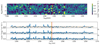 |
Fig. A.1. X-Shooter NIR spectrum of the HZ1 galaxy. Top panel shows the combined, rebinned (∼ 85 km s−1), and smoothed (0.7 nm × 0.12 ″) 2D spectrum. The bottom three panels illustrate the extracted 1D spectra rebinned by ∼ 210 km s−1, ∼ 170 km s−1, and ∼ 140 km s−1, respectively. Expected positions of the [CIII]λ1907 at λ = 1276.9 nm and CIII]λ1909 line at λ = 1275.6 nm, based on the Lyα spectroscopic redshift, are shown as yellow and red lines, respectively. Shaded blue regions indicate the flux, dotted lines indicate the uncertainties, whereas the orange solid line is the best Gaussian fit. |
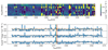 |
Fig. A.2. X-Shooter NIR spectra of the RXJ 1347-1216 galaxy. Top panel shows the combined, rebinned (∼ 75 km s−1), and smoothed (0.7 nm × 0.12 ″) 2D spectrum. The bottom three panels illustrate the extracted 1D spectra rebinned by ∼ 180 km s−1, ∼ 145 km s−1, and ∼ 120 km s−1, respectively. Expected positions of the [CIII]λ1907 at λ = 1480.7 nm and CIII]λ1909 line at λ = 1482.3 nm, based on the Lyα spectroscopic redshift, are shown as yellow and red lines, respectively. Labels are the same as in Fig. A.1. |
 |
Fig. A.3. X-Shooter NIR spectra of the GDS3073 galaxy. Top panel shows the combined, cropped, and smoothed (0.7 nm × 0.12 ″) 2D spectrum. The bottom three panels illustrate the extracted 1D spectra rebinned by ∼ 180 km s−1, ∼ 145 km s−1, and ∼ 120 km s−1, respectively. Expected positions of the [CIII]λ1907 at λ = 1251.4 nm and CIII]λ1909 line at λ = 1252.7 nm, based on the Lyα spectroscopic redshift, are shown as yellow and red lines, respectively. Labels are the same as in Fig. A.1. |
 |
Fig. A.4. X-Shooter NIR spectra of the UVISTA-Z-002 galaxy. Top panel shows the combined, rebinned (∼ 75 km s−1), and smoothed (0.7 nm × 0.12 ″) 2D spectrum. The bottom three panels illustrate the extracted 1D spectra rebinned by ∼ 180 km s−1, ∼ 145 km s−1, and ∼ 120 km s−1, respectively. Expected positions of the [CIII]λ1907 at λ = 1477.7 nm and CIII]λ1909 line at λ = 1479.2 nm, based on the Lyα spectroscopic redshift, are shown as yellow and red lines, respectively. |
In Fig. A.5, we show stacked 1D spectrum of six z ∼ 2 galaxies from the MUSE sample. The stacked spectrum is the weighted average of the rest-frame UV spectra of the six z ∼ 2 galaxies. The 1D spectra are rebinned to a have identical spectral resolution set to Δλ = 0.05 nm. We partially remove the skyline emission from the 1D spectra by subtracting the individual 1D galaxy spectrum by the 1D spectrum extracted from a r = 5″ region close to the galaxy. Wavelengths with skyline contamination are shown as vertical gray regions.
 |
Fig. A.5. Stacked 1D spectrum of six z ∼ 2 galaxies from the MUSE sample. The stacked spectrum is the weighted average of the rest-frame UV spectra of the six galaxies. The spectral resolution is set to Δλ = 0.05 nm. Rest-frame positions of the [CIII]λ1907 and CIII]λ1909 line are shown as yellow and red lines, respectively. Wavelengths with skyline contamination are shown as vertical gray regions. |
Appendix B: Posterior distributions of the ISM parameters
We report the corner plot (Foreman-Mackey 2016) that illustrates the 1D and 2D projections of the posterior probability distribution of the ISM parameters: log(n[cm−3]), log(Z[Z⊙]), and log(κs), for the HZ10 galaxy. For the total gas density log(n) parameter, we set an upper limit on the prior log(n[cm−3]) = 3.5, namely, a value close to the critical density of the emitting gas (e.g., Ferrara et al. 2019). Although it might be possible for the MCMC walkers to go beyond this limit, sources with such high mean density are not very probable, because this would imply that the average density of the galaxy is much higher than the typical average density of n ≈ 300 cm−3 found for high-z mock galaxies from the SERRA simulations (Pallottini et al. 2019).
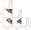 |
Fig. B.1. Corner plot representation of the posterior distribution of the ISM parameters: log(n[cm−3]), log(Z[Z⊙]), and log(κs) for the HZ10 source. The median of the posterior distribution and 1σ uncertainties are represented as orange solid and black dashed lines, respectively. |
Appendix C: ISM properties of sources with upper limits on carbon lines
Most of the sources of our sample have upper limits on either the C III] or [C II] emission. To be able to derive their ISM properties using the Vallini et al. (2020) model, we need to treat the upper limits on the carbon line as measured values and we assume that the uncertainties are equal to 25% of the upper limit estimates. With this procedure, we derive the κs, Z, and n parameters. The derived values for these sources are given in Table C.1.
Burstiness parameter κs, gas metallicity Z, and density n for galaxies with upper limits on either C III] or [C II] emission.
All Tables
Overview of the full galaxy sample used in this paper, grouped by C III] and [C II] detection.
UV radius, observed and intrinsic C III] line emission flux, C III] intrinsic luminosity, and surface brightness of the full galaxy sample.
βUV slope and UV attenuation at 1900 Å for three z > 5 galaxies with C III] and [C II] detections.
[C II] radius, luminosity and surface density, and total SFR, and SFR per unit area of the full galaxy sample.
Burstiness parameter κs, gas metallicity Z, and gas density n for the three z > 5 galaxies detected in both C III] and [C II].
Burstiness parameter κs, gas metallicity Z, and density n for galaxies with upper limits on either C III] or [C II] emission.
All Figures
|
Fig. 1. SFR vs. stellar mass of our full galaxy sample. Sources at 5.5 < z < 7.5 with new and archival C III] data, galaxies at z ∼ 2 with archival C III] data, and literature sample at 6.0 < z < 7.5 are shown as blue, green, and orange circles, respectively. The best-fit relations for the main sequence (MS) at 5.5 < z < 7.5 and 1.7 < z < 2.0 from Schreiber et al. (2015) are shown as magenta and red bands, respectively. SFR and stellar mass references: HZ1, HZ10 – Capak et al. (2015); RXJ 1347−1216 – Huang et al. (2016), Bradač et al. (2017); GDS3073 – Grazian et al. (2020); UVISTA-Z-002 – Bowler et al. (2017a), Bouwens et al. (2022); COS-3018 – Smit et al. (2018); A383-5.2 – Matthee et al. (2019), Stark et al. (2015); z7_GND_42912 – Schaerer et al. (2015); Himiko – Carniani et al. (2018b), Graziani et al. (2020); CR7, CR7a, CR7b, CR7c – Matthee et al. (2017a); Bowler et al. (2014, 2017b); COS-13679 – Matthee et al. (2019), Laporte et al. (2017); COS-2987 – Smit et al. (2018), Laporte et al. (2017); VR7 – Matthee et al. (2019, 2017b); 9347, 6515, 10076, 9834, 9681, 8490 – this work, Zanella et al. (2018). |
| In the text | |
|
Fig. 2. X-shooter NIR spectrum of the HZ10 galaxy. Top panel: combined, rebinned (≈ 85 km s−1), and smoothed (1.1 nm × 0.12″) 2D spectrum. The C III] λλ1907, 1909 line is detected in the center of the slit with the negative flux on each side. The bottom three panels illustrate the extracted 1D spectra rebinned by ≈ 210 km s−1, ≈ 170 km s−1, and ≈ 140 km s−1, respectively. Shaded blue regions indicate the flux, dotted lines indicate the uncertainties, whereas orange solid line is the best Gaussian fit. Expected positions of the [C III] λ1907 at λ = 1269.7 nm and [C III] λ1909 line at λ = 1271.0 nm, based on the Lyα spectroscopic redshift, are shown as yellow and red lines, respectively. |
| In the text | |
|
Fig. 3. [C II] surface brightness Σ[C II] vs. C III] surface brightness Σ[[C III], color-coded by the SFR per unit area ΣSFR, for our entire sample of galaxies. Sources that are detected both in [C II] and C III] are annotated. |
| In the text | |
|
Fig. 4. [C II] surface brightness vs. SFR per unit area, color-coded by the C III] surface brightness, of this sample of galaxies. Filled and empty circles indicate sources with the C III] line detection and upper limits, respectively. Galaxies detected both in [C II] and C III] emission are annotated. Blue × symbols indicate a subsample of galaxies from the ALPINE survey at 4 < z < 6 (Le Fèvre et al. 2020). Σ[C II] − ΣSFR relation for local galaxies by De Looze et al. (2014) is represented as a blue dashed line with a 1σ dispersion of 0.32 dex. This relation is extrapolated to cover the distribution of high-z sources in Σ[C II] − ΣSFR space, which is shown as a light-blue dashed line. Σ[C II] − ΣSFR relation predictions from models of Ferrara et al. (2019) with three different combinations of fixed κs, Z, and n parameters (Table 5) are represented as dotted gray lines. Finally, the best-fit model (Z = 0.24 Z⊙, log(n[cm−3]) = 2.98, and log(κs) ≈ 1.30) on all the galaxies (excluding Z7_GND_42912) and 100 random samples from the MCMC chain are shown as thick and thin purple solid lines, respectively. |
| In the text | |
|
Fig. 5. Deviation from the local Σ[C II] − ΣSFR relation Δ vs. the C III] over [C II] surface brightness ratio, color-coded by the SFR per unit area ΣSFR. Galaxies detected both in [C II] and C III] emission are annotated. We plot a grid of model predictions with fixed metallicity and gas density, with the burstiness parameter varying in a range of 0 ≤ log(κs) ≤ 2.4 i.e., κs = 1, 5, 10, 30, 50, 100, 250 (dotted lines), and log(ΣSFR[M⊙ yr−1]) in −0.5 ≤ log(ΣSFR[M⊙ yr−1]) ≤ 2.5 (solid lines). The top panel shows an example of a model prediction for high-z galaxies with ISM properties similar to HZ10, with solar metallicity Z = Z⊙ and gas density close to critical density of log(n[cm−3]) = 3.3. Bottom panel shows predictions for typical high-z galaxies with subsolar metallicity Z = 0.5 Z⊙ and log(n[cm−3]) = 2.5. |
| In the text | |
|
Fig. 6. Burstiness parameter κs vs. deviation from the local De-Looze relation Δ, color-coded by the C III] surface brightness ΣC III]. Galaxies detected both in [C II] and C III] emission are annotated and represented as filled circles. Galaxies at 6 < z < 9 from Vallini et al. (2021) are represented as gray stars. Linear fit on the detected sources is shown as a blue line with 1σ uncertainties as a shaded region. |
| In the text | |
|
Fig. 7. Density of the emitting gas n vs. deviation from the local De-Looze relation Δ, color-coded by the C III] surface brightness Σ[[C III]. Symbols are the same as in Fig. 6. |
| In the text | |
|
Fig. A.1. X-Shooter NIR spectrum of the HZ1 galaxy. Top panel shows the combined, rebinned (∼ 85 km s−1), and smoothed (0.7 nm × 0.12 ″) 2D spectrum. The bottom three panels illustrate the extracted 1D spectra rebinned by ∼ 210 km s−1, ∼ 170 km s−1, and ∼ 140 km s−1, respectively. Expected positions of the [CIII]λ1907 at λ = 1276.9 nm and CIII]λ1909 line at λ = 1275.6 nm, based on the Lyα spectroscopic redshift, are shown as yellow and red lines, respectively. Shaded blue regions indicate the flux, dotted lines indicate the uncertainties, whereas the orange solid line is the best Gaussian fit. |
| In the text | |
|
Fig. A.2. X-Shooter NIR spectra of the RXJ 1347-1216 galaxy. Top panel shows the combined, rebinned (∼ 75 km s−1), and smoothed (0.7 nm × 0.12 ″) 2D spectrum. The bottom three panels illustrate the extracted 1D spectra rebinned by ∼ 180 km s−1, ∼ 145 km s−1, and ∼ 120 km s−1, respectively. Expected positions of the [CIII]λ1907 at λ = 1480.7 nm and CIII]λ1909 line at λ = 1482.3 nm, based on the Lyα spectroscopic redshift, are shown as yellow and red lines, respectively. Labels are the same as in Fig. A.1. |
| In the text | |
|
Fig. A.3. X-Shooter NIR spectra of the GDS3073 galaxy. Top panel shows the combined, cropped, and smoothed (0.7 nm × 0.12 ″) 2D spectrum. The bottom three panels illustrate the extracted 1D spectra rebinned by ∼ 180 km s−1, ∼ 145 km s−1, and ∼ 120 km s−1, respectively. Expected positions of the [CIII]λ1907 at λ = 1251.4 nm and CIII]λ1909 line at λ = 1252.7 nm, based on the Lyα spectroscopic redshift, are shown as yellow and red lines, respectively. Labels are the same as in Fig. A.1. |
| In the text | |
|
Fig. A.4. X-Shooter NIR spectra of the UVISTA-Z-002 galaxy. Top panel shows the combined, rebinned (∼ 75 km s−1), and smoothed (0.7 nm × 0.12 ″) 2D spectrum. The bottom three panels illustrate the extracted 1D spectra rebinned by ∼ 180 km s−1, ∼ 145 km s−1, and ∼ 120 km s−1, respectively. Expected positions of the [CIII]λ1907 at λ = 1477.7 nm and CIII]λ1909 line at λ = 1479.2 nm, based on the Lyα spectroscopic redshift, are shown as yellow and red lines, respectively. |
| In the text | |
|
Fig. A.5. Stacked 1D spectrum of six z ∼ 2 galaxies from the MUSE sample. The stacked spectrum is the weighted average of the rest-frame UV spectra of the six galaxies. The spectral resolution is set to Δλ = 0.05 nm. Rest-frame positions of the [CIII]λ1907 and CIII]λ1909 line are shown as yellow and red lines, respectively. Wavelengths with skyline contamination are shown as vertical gray regions. |
| In the text | |
|
Fig. B.1. Corner plot representation of the posterior distribution of the ISM parameters: log(n[cm−3]), log(Z[Z⊙]), and log(κs) for the HZ10 source. The median of the posterior distribution and 1σ uncertainties are represented as orange solid and black dashed lines, respectively. |
| In the text | |
Current usage metrics show cumulative count of Article Views (full-text article views including HTML views, PDF and ePub downloads, according to the available data) and Abstracts Views on Vision4Press platform.
Data correspond to usage on the plateform after 2015. The current usage metrics is available 48-96 hours after online publication and is updated daily on week days.
Initial download of the metrics may take a while.