| Issue |
A&A
Volume 663, July 2022
|
|
|---|---|---|
| Article Number | A58 | |
| Number of page(s) | 22 | |
| Section | Interstellar and circumstellar matter | |
| DOI | https://doi.org/10.1051/0004-6361/202142777 | |
| Published online | 14 July 2022 | |
Importance of source structure on complex organics emission
II. Do disks explain lack of methanol emission from low-mass protostars?
1
Leiden Observatory, Leiden University,
PO Box 9513,
2300 RA
Leiden, The Netherlands
e-mail: nazari@strw.leidenuniv.nl
2
School of Physics and Astronomy, University of Leicester,
Leicester
LE1 7RH,
UK
3
LERMA, Observatoire de Paris, Université PSL, CNRS, Sorbonne Université,
92195
Meudon, France
4
Max Planck Institut für Extraterrestrische Physik (MPE),
Giessenbachstrasse 1,
85748
Garching, Germany
Received:
29
November
2021
Accepted:
29
March
2022
Context. The protostellar stage is known to be the richest star formation phase in emission from gaseous complex organic molecules. However, some protostellar systems show little or no millimetre (mm) line emission of such species. This can be interpreted as a low abundance of complex organic molecules. Alternatively, complex species could be present in the system, but are not seen in the gas.
Aims. The goal is to investigate the second hypothesis for methanol as the most abundant complex organic molecule in protostellar systems. This work aims to determine how effective dust optical depth is in hiding methanol in the gas, and whether methanol can mainly reside in the ice due to the presence of a disk that lowers the temperatures. Hence, we attempt to answer the question whether the presence of a disk and optically thick dust reduce methanol emission even if methanol and other complex species are abundant in the ices and gas.
Methods. Using the radiative transfer code RADMC-3D, we calculated methanol emission lines from an envelope-only model and from an envelope-plus-disk model. We compared the results with each other and with the observations. Methanol gas and ice abundances were parametrised inside and outside of the snow surfaces based on values from observations. Both models included either dust grains with low mm opacity or high mm opacity, and their physical parameters such as envelope mass and disk radius were varied.
Results. Methanol emission from the envelope-only model is always stronger than from the envelope-plus-disk model by at least a factor ∼2 as long as the disk radius is larger than ∼30 au (for L = 8 L⊙). In most cases, this is due to lower temperatures (disk shadowing), which causes the smaller amount of warm (≳70 K) methanol inside the snow surface of the envelope-plus-disk model. The intensities drop by more than an order of magnitude for models including high mm opacity dust grains and disk radii of at least ∼50 au (for L = 8 L⊙) due to continuum over-subtraction.
Conclusions. The line intensities from the envelope-only models match the observations moderately well when methanol emission is strong, but they overproduce the observations of protostars with lower methanol emission even with large dust optical depth effects. The envelope-plus-disk models can explain the bulk of the observations. However, they can only reproduce the observations of sources with high luminosities and very low methanol emission when the dust optical depth is significant in the envelope and continuum over-subtraction becomes effective in the disk (high mm opacity dust grains are used). Therefore, both the effects of disk and dust optical depth should be considered to explain the observations. In conclusion, it is important to take physical structure into account in future chemical studies of low-mass protostars: absence of gas-phase methanol emission does not imply absence of methanol molecules in either gas or ice.
Key words: astrochemistry / stars: low-mass / stars: protostars / ISM: abundances / ISM: molecules / radiative transfer
© ESO 2022
1 Introduction
The protostellar phase of star formation is the stage at which most of the material surrounding the protostar is warm, and hence species existing in ices can sublimate into the gas phase and cause this stage to become the most line-rich stage (Herbst & van Dishoeck 2009; Caselli & Ceccarelli 2012; van’t Hoff et al. 2020). Therefore, the earlier stages of star formation provide the best opportunity to study complex organics in the gas phase.
Methanol (CH3OH) is the most common complex organic molecule detected towards both low- and high-mass protostars in the gas over the past decades (e.g. Blake et al. 1987; van Dishoeck et al. 1995; Gibb et al. 2000; Bisschop et al. 2007; Belloche et al. 2013; Jørgensen et al. 2016; Ilee et al. 2016; Bøgelund et al. 2018; Marcelino et al. 2018; Martín-Doménech et al. 2019; Taquet et al. 2019; van Gelder et al. 2020; Manigand et al. 2020; Yang et al. 2020; Ligterink et al. 2021; Law et al. 2021). Moreover, methanol has been observed to be abundant (XH ∼ 3 × 10⁻⁶, with some spread) in ices towards protostellar objects (Geballe et al. 1988; Dartois et al. 1999, 2002; Boogert et al. 2008, 2015; Bottinelli et al. 2010; Öberg et al. 2011) and in some dark cores prior to star formation (Boogert et al. 2011; Qasim 2020). A high methanol abundance in both gas and solids is only possible if methanol is formed in the ice as observed in laboratory experiments and chemical models (Hidaka et al. 2004; Geppert et al. 2006; Fuchs et al. 2009; Garrod & Pauly 2011).
However, some sources do not show methanol emission at millimetre (mm) wavelengths in the gas, which has become more apparent from the recent Atacama Large Millimeter/submillimeter Array (ALMA) and the Northern Extended Millimeter Array (NOEMA) surveys. Yang et al. (2021) detected methanol in 56% of their 50 low-mass protostars, and Belloche et al. (2020) detected methanol in 50% of the 26 low-mass protostars they observed.
This has been investigated further in van Gelder et al. (2022), who reported a spread of four orders of magnitude in the mass of gaseous methanol in protostars of similar luminosity that were observed by ALMA. This might mean that the amount of methanol strongly varies in the hot cores. Modelling work of Drozdovskaya et al. (2014) showed that the abundance of methanol can increase or decrease through infall and evolve from the prestellar core to the protoplanetary disk depending on the disk growth mechanisms. Hence, the spread in column density of methanol as found by van Gelder et al. (2022) might be partially explained by the loss of methanol during the infall or the destruction of methanol through some other process (dehydrogenation, when a molecule loses a hydrogen atom through some chemical reaction; Nourry & Krim 2015; photodissociation; Laas et al. 2011; McGuire et al. 2017; Notsu et al. 2021), resulting in simply a lower methanol number density in some protostellar systems. However, Aikawa et al. (2020) showed with their chemical models that even if pristine methanol is destroyed at the end of the dark cloud phase, it will be efficiently reformed in the ice via reaction of CH3 and OH once the collapse starts. Therefore, the possibility of the absence of methanol in protostellar systems is less likely, and hence another explanation is required.
There is a similar debate for water abundances in protostellar systems (Persson et al. 2012, 2016; Visser et al. 2013; van Dishoeck et al. 2021), which seem to be orders of magnitude lower than the abundance expected (∼10–4) from ice sublimation. Several explanations have been proposed for this discrepancy based on chemistry and physical structures of the regions in the literature. Notsu et al. (2021) reported that X-ray induced chemistry of water and other molecules such as methanol decreases the abundances of these molecules in the inner protostellar region. Moreover, Persson et al. (2016) showed that a disk significantly reduces the amount of gas and dust above 100 K, potentially lowering abundances of water by an order of magnitude. The same argument can be applied to methanol because its sublimation temperature is similar to that of water (∼100 K).
Thus, it is possible that methanol is not observed in the gas because this molecule resides in the ice. The fact that a disk can decrease the temperature has been discussed in the literature (Persson et al. 2016; Murillo et al. 2015). In particular, Murillo et al. (2018) observed DCO+, a cold gas tracer (D/H is enhanced at lower temperatures), behind the location of the disks in IRAS 16293-2422A and VLA 1623-2417. They concluded that the lower temperatures behind the disk caused by disk shadowing produce an environment that is favourable for the formation of deuterated species such as DCO+.
Another reason that methanol is not observed in the gas might be that dust attenuation blocks the methanol emission. This has been directly observed by De Simone et al. (2020) for the case of NGC 1333 IRAS 4A1, where they detected methanol at centimetre wavelengths, while the same source did not show any complex organic emission at millimetre wavelengths (López-Sepulcre et al. 2017). Therefore, sources that appear poor in complex organic molecules with ALMA may in fact be rich in gaseous species, but they are hidden at ALMA wavelengths.
In this work, we investigate the scenario in which methanol is plentiful in the protostellar systems, but cannot be seen in the gas phase: could the drop in temperature caused by a disk in addition to dust optical depth explain the lack of gaseous methanol emission in some sources? To answer this, we compare the results of two different models: an envelope-only model, and a flattened envelope-plus-disk model. In both cases, we considered optically thin and thick mm continuum to examine the effects of dust attenuation as observed by De Simone et al. (2020). Methanol ice and gas abundances are simply parametrised in the models based on the values from observations and inspired by detailed chemical disk models and are not calculated by including a complete chemical network.
In Sect. 2, the models and the assumptions made are explained. Section 3 presents the results especially for the thermal structure and the methanol emission from the models. In Sect. 4, we discuss our findings and compare our results with observations of protostars with ALMA. Finally, Sect. 5 presents our conclusions.
2 Methods
2.1 Physical Structure
In the next two subsections, we describe the physical structures of the two models considered: the envelope-only and the envelope-plus-disk models.
2.1.1 Envelope-only Model
The left panel of Fig. 1 shows the density structure of our fiducial envelope-only protostellar system with an envelope mass of 1 M⊙ and protostellar luminosity of 8 L⊙ (values similar to those for complex organic-rich low-mass protostars, e.g. L1448 IRS2 and L1448 IRS3; Mottram et al. 2017). The spherically symmetric envelope model assumes a power-law relation between the gas density and radius,
 (1)
(1)
where ρg is the gas density of the envelope, r is the radius in spherical coordinates, and ρ0 is the gas density at radius r0, which is parametrised by the envelope mass and assuming inner and outer radii of the envelope of 0.4 au and 104 au. α was fixed to 1.5 to represent the values found from observations of protostellar envelopes on scales of ∼500 au and larger (Kristensen et al. 2012). A gas-to-dust mass ratio of 100 was assumed to calculate the dust density.
An outflow cavity was also added to the model with the same shape as the outflow cavity in the envelope-plus-disk model explained in Sect. 2.1.2. The density inside the cavity was fixed to 103 cm–3 to be in line with the observations (Bachiller & Tafalla 1999; Whitney et al. 2003).
A 5000 K blackbody was assumed for the input radiation field to mimic the effect of accretion luminosity and protostellar radiation field. The envelope mass was varied from 0.1 M⊙ to 10 M⊙ and the luminosity from 0.5 L⊙ to 32 L⊙. The envelope masses and luminosities were chosen so that they represent well-studied Class 0 objects (Jørgensen et al. 2009; Kristensen et al. 2012). Table 1 summarises the parameters we used for the envelope-only model.
2.1.2 Envelope-plus-disk Model
A disk was included through a parametrised disk plus a flattened envelope model following Crapsi et al. (2008) and Harsono et al. (2015). A sketch of the envelope-plus-disk physical structure is shown in Fig. 2, and the density structure for our fiducial envelope-plus-disk protostellar system with an envelope mass of 1 M⊙, a stellar luminosity of 8 L⊙, a disk radius of 50 au, and a disk mass of 0.01 M⊙ is shown in the right panel of Fig. 1. The disk mass and radius for the fiducial envelope-plus-disk model were chosen so that they agree with the values for typical Class 0 sources (Murillo et al. 2013; Maury et al. 2019; Tobin et al. 2020).
The gas density of the flattened envelope following Ulrich (1976) is
 (2)
(2)
where r is the radius in spherical coordinates, rout is the outer radius, rc is the centrifugal radius, which has been assumed to be 50 au, and θ0 is the initial latitude of each particle. The term cos θ0 was calculated for each point of the grid by solving the following equation:
 (3)
(3)
An outflow cavity was added to the model in a similar way as to the envelope-only model: by fixing the hydrogen density to 103 cm–3, where cos θ0 from Eq. (3) is higher than 0.95 to be consistent with the observations and modelling of outflows (Crapsi et al. 2008; Plunkett et al. 2013; Harsono et al. 2015).
A disk was added to the flattened envelope with a power-law gas density in radius and a Gaussian distribution in z direction in cylindrical coordinates expected from hydrostatic equilibrium. The density is given by (Shakura & Sunyaev 1973; Pringle 1981)
![${\rho _{{\rm{g,D}}}} = {{{M_{\rm{D}}}{{\left( {{R \mathord{\left/ {\vphantom {R {{R_{\rm{D}}}}}} \right. \kern-\nulldelimiterspace} {{R_{\rm{D}}}}}} \right)}^{ - 1}}} \over {\sqrt {8{\pi ^3}} H\left( R \right)R_{\rm{D}}^2}}\exp \left[ {{1 \over 2}{{\left( {{z \over {H\left( R \right)}}} \right)}^2}} \right],$](/articles/aa/full_html/2022/07/aa42777-21/aa42777-21-eq4.png) (4)
(4)
where MD is the disk mass, RD is the disk radius, z is the height from the disk mid-plane, R is the radius in cylindrical coordinates, and H(R) is the scale height of the disk, which is dependent on the radius. The disk radius, RD, is the physical size of the disk and is different from the gas and dust disk sizes measured from the observations, with gas sizes generally larger than those of the dust. H(R) is set by the thermal structure of the disk. The disk density was assumed to be zero at radii larger than the disk radius. When we assume a vertically isothermal disk, the scale height is given by εR, where ε is the aspect ratio of the disk and was fixed to 0.2 (Chiang & Goldreich 1997).
The total gas density in the envelope-plus-disk model is given by
 (5)
(5)
In Eq. (5), the outflow cavity and the envelope are assumed to be part of the same component, represented by ρg,E. The dust density was calculated by assuming a gas-to-dust mass ratio of 100.
The most important parameters of the disk are its mass and radius. We varied these two parameters as shown in Table 1. The disk mass and radius were varied simultaneously to keep  (an approximation to the disk surface density) constant in all models. The envelope mass and protostellar luminosity were varied in the same way as in the envelope-only models (see Sect. 2.1.1).
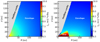 |
Fig. 1 Density profiles explored in this work. Left panel: 2D hydrogen nucleus number density, nH = n(H) + 2n(H2), for the fiducial envelope-only model. Right panel: Same as left panel, but for the fiducial flattened envelope-plus-disk model. In this figure and throughout, log is in base 10. |
Model parameters.
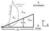 |
Fig. 2 Cartoon of the physical structure of the envelope-plus-disk model. H(R) and RD are the disk scale height and the disk radius. Din and Dout are the inner and outer part of the disk with respect to the sublimation surface. Ein and Eout are the same, but for the envelope. |
2.2 Methanol Abundance
The aim of this work is to calculate the emission from gasphase methanol in protostellar systems. Therefore, it is crucial to have a realistic model for the methanol abundance. This is parametrised in the models based on the various regions of the disk and envelope. These regions are marked in Fig. 2: Ein and Eout are the inner and outer envelope regions, and Din and Dout are the inner and outer disk regions, where inner means inside of the sublimation surface, and outer means outside of it.
We used the balance between adsorption and thermal desorption of methanol (Hasegawa et al. 1992) to calculate the snow surface and hence abundance (X) with respect to nH = n(H) + 2n(H2) at each point in the envelope-only model and in the envelope-plus-disk model. The ice-to-gas abundance ratio of methanol (Xice/Xgas) is equal to the ratio of the number density of the molecules in the solid phase to the gas phase, which is given by
 (6)
(6)
where ad is the characteristic dust grain size (see Appendix B); nd is the dust number density; S is the sticking coefficient, which is assumed to be 1; kB is the Boltzmann constant; Tgas is the gas temperature; Td is the dust temperature, which is assumed to be the same as Tgas due to thermal coupling of the gas and dust in the dense regions; mi is the mass of the species i; Eb is the binding energy, which is assumed to be 3820 K for methanol (Penteado et al. 2017); and nss is the number of binding sites per surface area, which is assumed to be 8 × 1014cm–2 (Visser et al. 2011). These values result in a desorption temperature of ∼70 K for the typical densities of our models (nH ∼ 107 cm–3).
A total methanol abundance (Xice + Xgas) of 10–6 was assumed in the envelope-only model and in the envelope component of the envelope-plus-disk model. Moreover, when Xgas reached below 10–9, the gas-phase abundance was set to 10–9 (i.e. the abundance in Eout in Fig. 2) to consider the non-thermal desorption mechanisms and gas-phase formation of methanol. Inside the disk, we used lower values of Xice + Xgas = 10–8 and a minimum of 10–11 (i.e. the abundance in Dout in Fig. 2). These values were chosen to match the observations of methanol ice (Boogert et al. 2015) and gas (Maret et al. 2004; Jørgensen et al. 2005) in warm regions of protostars and cold dark clouds (Sanhueza et al. 2013; Scibelli et al. 2021) for the envelope component, and to match observation and modelling of Class II disks (Walsh et al. 2014; Booth et al. 2021; Gavino et al. 2021) for the disk component.
The value of 10–6 for the envelope is mainly based on the ice abundances found in Boogert et al. (2015), although a spread of a factor ∼3 is observed in the methanol ice abundances in protostars (Öberg et al. 2011). The gas-phase abundances of methanol in hot cores are uncertain due to the large uncertainty on the warm hydrogen number density. For example, Jørgensen et al. (2016) reported a value of 1.5 × 10⁻⁶ for the methanol abundance with respect to total H and argued that this value is an upper limit due to the uncertainty on the column density of total H found from the optically thick continuum. Hence, using a value for the methanol abundance in the inner envelope based on the ice abundances in the outer envelope is the best that can be done.
The photodissociation of methanol by UV radiation was taken into consideration by setting the methanol abundance to zero where the UV optical depth (τUV) at 1500 Å (the wavelength at which methanol is effectively photodissociated; Heays et al. 2017) is lower than 3 (i.e. Av ≲ 1 for small grains). This mimics photodissociation due to the UV excess from the accreting protostar or UV produced in fast jet shocks (e.g. HH46; van Kempen et al. 2009 and in HH211; Tabone et al. 2021). We note that this UV excess was not explicitly added to the radiation field since no chemistry model was included: only its penetration depth into the envelope was considered. The UV optical depth was calculated by first calculating the UV radiation field at wavelength of 1500 Å in RADMC-3D version 2.01 with dust (Fuv) and without dust (FUV,0) to be used as a reference. Then, τUV was found by –ln(FUV/FUV,0) (Visser et al. 2011). This procedure resulted in a thin layer next to the cavity wall in which methanol is absent for low mm opacity dust grains (corresponding to a high UV opacity; see Fig. A.1) and a thicker layer for high mm opacity dust grains (corresponding to low UV opacity). Moreover, at radii < 1 au, the methanol abundance was set to zero assuming that methanol is thermally destroyed very close to the protostar.
2.3 Temperature and Line Emission Calculations
An accurate calculation of the thermal structure of the system is crucial as the temperature sets the sublimation region of methanol and the excitation conditions. The dust and the gas were assumed to be thermally coupled given that the studied regions have high densities. The dust temperature was calculated using Monte Carlo dust continuum radiative transfer by propagation of photons from the central star. We used the code RADMC-3D version 2.0 for this calculation. The temperature structure and dust opacity depend on the optical properties of the dust. We used two dust distributions, one at a time for a model. The two dust distributions encompass the range of variation in opacity at the studied wavelengths (∼1 mm) depending on assumptions on grain size and composition (see Fig. A.1 and Ysard et al. 2019). The first distribution consists of small silicate grains (amorphous olivine) with a dust size of 0.1 µm and a bulk density of 3.7 g cm–3 (κ1 mm ≃ 0.2 cm2 g–1). The second includes larger grains with a dust distribution ∝ a–35, a maximum dust size of 1 mm, a minimum dust size of 50 Å, and a composition that includes water ice and amorphous carbon in addition to amorphous olivine, with an average bulk density over all components of 1.4 g cm–3 (κ1 mm ≃ 18 cm2 g–1). For the remainder of this paper, the first dust distribution is referred to as low mm opacity dust, and the second dust distribution is referred to as high mm opacity dust. The symbol κdust in this paper always refers to opacity at mm wavelengths unless otherwise stated.
The spatial grid was logarithmically spaced in the r direction and linearly spaced in the θ direction for the envelope-only and envelope-plus-disk models. In the calculation of temperature, isotropic scattering was switched on in RADMC-3D (see Fig. A.1 for the albedo of the dust grains). The number of grid cells and photons we used to calculate the temperature was varied to reach convergence in the temperature structure in the models. The final number of grid cells used in the envelope-plus-disk model in the r direction was 300 for radii between 0.4 au and 0.5 au and 700 for radii between 0.5 au and 104 au, whereas 400 cells were used in the θ direction. For the envelope-only model, 1000 grid cells were used in the r direction and 400 in the θ direction. Both models assumed azimuthal symmetry. In both models, the number of photons used for temperature calculation was 106. Multiple tests showed that this number of photons yields accurate temperatures while keeping the computational time to a minimum.
After the continuum radiative transfer and temperature calculation, line radiative transfer was done by ray tracing from the protostar to the observer using the RADMC-3D version 2.0 “circ image” command. In this calculation, we assumed local thermodynamic equilibrium (LTE), which is reasonable given the densities inside the snow line (see Appendix C for more details of the critical density needed for LTE conditions). The effects of non-LTE calculation on the models are further investigated in Sect. 4.2. The molecular data needed in ray tracing of A-CH3OH (as opposed to its E symmetry, which is determined by the nuclear spin alignment of the hydrogen atoms in CH3) was taken from the Leiden Atomic and Molecular Database (Schöier et al. 2005). For this file, the energy levels, Einstein A coefficients and transition frequencies were taken from the Cologne Database for Molecular Spectroscopy (CDMS; Müller et al. 2001, Müller et al. 2005; Xu et al. 2008), and the collisional rate coefficients were taken from Rabli & Flower (2010). The methanol line CH3OH 51,4-41,3 with a frequency of 243.916GHz (Eup = 49.7 K, Aij = 6.0 × 10⁻⁵ s–1) is studied in this work. This line was chosen because it is observed as part of the Perseus ALMA Chemistry Survey (PEACHES) towards low-mass protostars (Yang et al. 2021) and hence, it is possible to compare our findings with these observations.
To calculate the emission lines, the synthetic images were produced up to velocities of ±15 km s–1 around the centre of the desired methanol line. The velocity bin (i.e. spectral resolution) we used is 0.2 km s–1. A range of viewing angles were considered, going from a completely face-on source to a completely edge-on source. Moreover, during the ray tracing, both gas and dust were included in the models, and later, the spectral lines were continuum subtracted when we measured the integrated intensities. Isotropic scattering was switched on for the case of high mm opacity grains and was switched off for low mm opacity grains during the ray tracing. The reason for this is that when the grains have low mm opacity (they are small), there is no difference between the emission lines when the scattering is included or excluded (see Fig. A.1), and switching scattering off will decrease the computation time. Again, a convergence test was made to indicate the number of photons needed for scattering during the ray tracing for models with high mm opacity dust grains. The number of photons used for scattering during the ray tracing in the final models was 105. To generate the spectral lines, we integrated the emission over an area with 2″ diameter (300 au at the assumed source distance of 150pc) to mimic the typical spatial resolution of submillimetre surveys, in which most sources are unresolved. This assumed area introduces an uncertainty for some models when the integrated flux from the 2″ area is compared to the true integrated flux over which warm methanol is emitting. However, this uncertainty is a factor ≲2 for most of the models considered in this work. This uncertainty increases to a factor ∼3 underestimate for some extreme cases, such as the models with the highest luminosity and a low envelope mass. Similarly, the amount is overestimated for example for the lowest luminosity cases with a high envelope mass. However, these cases do not dominate the sample of models. The area of the 100 K radius that Bisschop et al. (2007) used to calculate the beam dilution factor for their observations for most of the models is well within the area assumed here (i.e. the 100 K radius is usually smaller than a 1″ radius; also see van’t Hoff et al. 2021 for low-mass sources).
A turbulent velocity of 1 km s–1 was assumed in the envelope component of the two models, and 0.1 km s–1 was assumed in the disk component of the envelope-plus-disk model. We assumed no free-fall velocity for simplicity because we are only interested in the integrated line fluxes rather than the small-scale kinematical structure of the envelope. However, in the disk component, Keplerian velocity  was assumed. These values in the two models result in a full width at half maximum (FWHM) of ∼2 km s–1 for the emission lines that are similar to what is observed for young protostars (see Jørgensen et al. 2005).
3 Results
3.1 Thermal Structure and the Snow Surfaces
Figure 3 presents the temperature structure of the envelope-only model in the left and the temperature structure of the envelope-plus-disk model in the middle column. The comparison of the radial temperature profiles of the two models through the mid-plane is shown in the right column. The top row shows the temperature structure for the fiducial envelope-only and envelope-plus-disk models: MD = 0.01 M⊙, RD = 50 au, ME = 1 M⊙, and L⋆ = 8 L⊙ with the low mm opacity dust grains. The bottom row corresponds to the same set of models including large dust grains, which are representative of dust with high opacity in the millimetre (large κdust).
The third column in the first row shows that the temperature structure of the envelope-only model approximately follows a power law (with an exponent of ∼–0.5) in the outer envelope, where dust is optically thin to the reprocessed far-IR and mm wavelengths from other grains. This is consistent with the expected scaling with the optically thin assumption at the Rayleigh-Jeans limit. However, in the inner envelope, where dust is optically thick to the reprocessed shorter wavelengths, radiative transfer modelling becomes crucial and the profile becomes steeper than the scaling suggests. This is consistent with what Jørgensen et al. (2002) found in their envelope-only models. In the envelope-plus-disk model, at large radii (≳200 au), the temperature profile follows a power law similar to the envelope-only model, but at lower temperatures. At the small radii at which the disk is located, the temperature difference between the two models is more significant.
In the upper layers of the disk, the temperature is highest and in the mid-plane it is lowest. The disk is heated by passive irradiation from the protostar and reprocessing by dust (Chiang & Goldreich 1997; Dullemond et al. 2001). The effect of disk shadowing is to lower the temperature beyond the outer edge of the disk at radii larger than ∼50 au.
Comparing the two rows, the temperature profiles are similar for the two dust distributions, with the methanol snow surface at ∼70 K being slightly closer to the central protostar when the dust has a high mm opacity. This is expected because of two effects. First, dust with high mm opacity is less efficient in absorbing UV and optical light (low dust opacity at UV and optical wavelengths). This especially affects the outflow cavity walls and the disk surface, which are directly irradiated by the visible and UV photons from the protostar. Therefore, these regions are colder when the dust has a high mm opacity. Second, when the grains with high mm opacity absorb the radiation at each point, they are more efficient at re-emitting it at longer wavelengths than the dust that has low mm opacity. The differences in snow surface around the outflow cavity walls are related to the first effect, while those in the disk mid-plane are more related to the second effect. The other parameters of the disk and the envelope, such as mass and disk radius, also have effects on the temperature structure. These effects are shown in Appendix D.
Figure 4 shows the gas-phase methanol abundance maps for the same models as in Fig. 3. This plot shows more clearly where methanol is sublimated from the grains. In particular, most of the warm methanol in the disk is located in the hot upper layers and not in the cold mid-plane, as expected. Moreover, this figure shows the photodissociation region of methanol near the cavity edge, which is larger in spatial extent when dust grains with high mm opacity are used. These dust grains are more optically thin to the UV radiation.
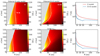 |
Fig. 3 Two-dimensional dust temperatures in the envelope-only models (left column) and in the envelope-plus-disk models (middle column). The white contours show the location in which the temperature is 70 K as an indication of the approximate temperature at which methanol is sublimated at the densities of the models. The right column compares the mid-plane temperature in the envelope-plus-disk models and the envelope-only models. The first row presents the fiducial model, and the second row presents the fiducial model with high mm opacity dust grains. In all figures in this work, κdust refers to the opacity of the dust grains at mm wavelengths. On average, the temperatures are lower when a disk is present and when grains have high mm opacity. |
3.2 Warm Methanol Mass
In Fig. 3, the location of the methanol snow surface is shown. In Sect. 3.1, we discuss its dependence on various model parameters, especially the presence of a disk. Due to the differences in the snow surface locations, the warm methanol mass inside the snow surface is expected to vary. The warm methanol mass is a relevant value as it is directly proportional to the methanol emission when the spectral line is optically thin.
Figure 5 presents the warm methanol mass, that is, the amount of methanol inside the snow surface as a function of disk radius (left panel), envelope mass (middle panel), and luminosity (right panel). In the left panel, the disk mass is varied simultaneously with the disk radius to ensure that the value of  (an approximation for the disk surface density) stays constant in all models so that only the effect of disk radius and not the changes in surface density are shown.
The first point to note is that the warm methanol mass increases with envelope mass and luminosity. The relation with respect to luminosity is in the form of a power-law. The slope of this relation in logarithmic space agrees well with the three-fourths exponent in the analytical relation of  (see Appendix B of Nazari et al. 2021 for the derivation; van Gelder et al. 2022). The reason for this is that the snow surface moves farther from the star when the luminosity increases (Fig. D.1). For an increasing envelope mass but constant luminosity, the warm methanol mass increases simply because of the higher density of the envelope, so that within the same volume, there is more methanol mass.
The warm methanol mass increases mildly with disk radius when the dust grains have a high mm opacity, but stays constant with increasing disk radius when dust grains have a low mm opacity. For low mm opacity grains, the warm mass is dominated by the envelope component, as shown in Fig. E.1. As the disk radius increases, the snow surface approaches the protostar (Fig. E.4) such that the mass decreases in the envelope component and increases in the disk component, so that the total warm mass stays roughly constant. For high mm opacity dust grains, the larger photodissociation regions affect the warm mass in the envelope component more than the disk component, therefore the warm mass is dominated by the disk component, as shown in Fig. E.2. Therefore, increasing the disk radius will increase the warm mass.
In the models with low mm opacity dust grains, the warm methanol mass is always higher in the envelope-only models than the envelope-plus-disk models. This is due to the lower temperatures of the models with disks, especially in the disk mid-plane, and beyond where the disk is located due to the disk-shadowing effect.
In the models with large κdust at mm wavelengths, the warm mass in the envelope-plus-disk models is generally lower than that in the models without a disk, except for the models with ME of 0.1 M⊙ and 0.3 M⊙ (see the large drop in warm methanol mass at low envelope masses in the middle column). In these cases, due to the low envelope masses, most of the methanol is photodissociated when the grains have high mm opacity (low UV opacity). However, these envelope masses are at the lower limit or extreme of those observed in Class 0 sources (Kristensen et al. 2012).
Comparison between the envelope-only models with small and large κdust at mm shows that the methanol mass is mainly about twice lower when the grains have large κdust. This is because of two effects. First, the snow surfaces of the models with high mm opacity grains are closer in than those for low mm opacity grains (see Fig. 3), but this has a small effect. Second, the photodissociation region of methanol is larger when the mm opacity of the dust is high. However, this drop in warm methanol mass in the envelope-only models between the high and low mm opacity dust grains does not seem to hold when the envelope mass is >1 M⊙ (Fig. 5, middle panel). This is because the dissociation regions become more similar between the models with high and low mm opacity grains once the envelope mass increases. This is expected because with higher densities, it is harder for the UV light to penetrate, and at a threshold of ∼3 M⊙, the photodissociation regions make up a small fraction of the warm envelope (see Fig. E.3).
Finally, the spread seen in the warm methanol mass for the models shown in Fig. 5 is between ∼10–10 M⊙ and ∼10–7 M⊙, which agrees well with the results of van Gelder et al. (2022) from observations of Class 0 objects by ALMA.
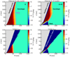 |
Fig. 4 Methanol abundance maps for the envelope-only (left) and envelope-plus-disk (right) models. The magenta contours show where the temperature is 70 K to indicate where the approximate sublimation surfaces of methanol are at the densities in the models. The photodissociation region (τUV < 3) is much larger in the envelope for the dust distribution with high mm opacity. |
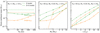 |
Fig. 5 Change in warm methanol mass with disk radius (left panel), envelope mass (middle panel), and luminosity (right panel). The dashed lines show the envelope-only models, and the solid lines show the envelope-plus-disk models. The fiducial models are indicated by a cross. The warm methanol mass is computed inside the methanol snow surface where the methanol abundance is higher than 10–9 in the envelope and higher than 10–11 in the disk (i.e. the methanol mass in Din and Ein in Fig. 2) for models with low mm opacity dust grains (green) and high mm opacity dust grains (orange). In the models in which RD is varied, luminosity and mass of the envelope are fixed to 8 L⊙ and 1 M⊙. The dashed lines are constant in the left panel because the envelope-only models do not have a disk for which its radius can be altered. Where ME is varied, the luminosity, disk mass, and radius are fixed to 8 L⊙, 0.01 M⊙, and 50 au. Where the luminosity is varied, the envelope mass, disk mass, and radius are fixed to 1 M⊙, 0.01 M⊙, and 50 au. |
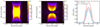 |
Fig. 6 Methanol emission for the fiducial models (low mm opacity dust). The left panel shows the emission from methanol at the peak of the line (0 km s–1) for the envelope-only model viewed edge-on, and the middle panel shows the same for the envelope-plus-disk model. Because no free-fall velocity is assumed, the line profile is nearly Gaussian with no infall signatures and thus, the emission at the peak of the line is similar to the integrated intensity map of the line. The right panel is the comparison between the line emission from the envelope-only model and the envelope-plus-disk model seen face-on (dashed lines) and edge-on (solid lines) after integrating over a 2″ diameter emitting area (300 au at the assumed source distance of 150 pc). |
3.3 Methanol Emission
3.3.1 Sample Emission Lines
The goal of this work is to compare the methanol emission in the two models with and without a disk. Figure 6 shows the line emission from the fiducial models in an edge-on view for the line at a frequency of 243.916 GHz. The left panel shows the emission at 0 km s–1 for the envelope-only model observed edge-on, the middle panel shows the same for the envelope-plus-disk model, and the right panel shows the respective emission lines seen edge-on (solid lines) and face-on (dashed lines).
The right panel of Fig. 6 shows that the peak of the line flux for the envelope-only model is ∼1.3 times the flux peak for the envelope-plus-disk model when observed edge-on. Because of the similar line widths, the integrated line fluxes are also different by a factor ∼1.3. This difference can be understood by considering the amount of warm methanol in the envelope-only and in the envelope-plus-disk models in Fig. 5. For the fiducial models (crosses) in this figure, the warm methanol mass is about four times higher in the envelope-only model than the envelope-plus-disk model, and hence a lower methanol flux in the envelope-plus-disk model is expected. The difference of a factor four in the warm mass has translated into only a a difference of a factor ∼1.3 in the fluxes when observed edge-on and into an even smaller difference when observed face-on because of the line optical depth effects in the disk and envelope. We discuss this further in Sect. 4.1.
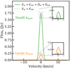 |
Fig. 7 Comparison of the spectral line emission of methanol from the envelope component of the envelope-plus-disk model (dotted lines) and emission from the envelope component and the disk component of the envelope-plus-disk model (solid lines). The line fluxes for the envelope component of the envelope-plus-disk model (dotted lines) were calculated by setting the abundance of methanol in the disk to zero. Green shows the fiducial model, i.e. low mm opacity dust grains, and orange shows the fiducial model with high mm opacity dust grains. |
3.3.2 Origin of Line Emission
Figure 7 presents the spectral line emission from the different components of the fiducial envelope-plus-disk model and the same model with high mm opacity dust grains viewed face-on (see Fig. 2 for the components). The emission is dominated by the envelope for both low and high mm opacity dust grains. For low mm opacity dust grains, this is due to the small amount of warm methanol in the disk component (Din) compared to the envelope component (Ein). The warm methanol mass from the various components of the fiducial envelope-plus-disk model is presented in Fig. E.1. However, when the grains have high mm opacity, the warm methanol mass is dominated by the disk component (see Fig. E.2), but the emission is still dominated by the envelope component. This is because of the continuum over-subtraction effect (explained in Sect. 4.1), where emission of methanol from the disk component is hidden by the optically thick dust in the disk.
Moreover, comparing the emission lines when κdust at mm is small with the case where κdust at mm is large, there is a drop of a factor of about seven in the peak of the line fluxes. Repeating the comparison for the warm methanol mass between the two models (Fig. 5) shows that the warm mass is only a factor ∼3.5 lower when the dust grains have a high mm opacity. Therefore, some part of the difference of a factor of about seven is due to the lower amount of warm methanol, which in turn is mainly caused by the larger photodissociation regions when grains have a high mm opacity. The remaining difference of a factor of about seven comes from the larger optical depth of the dust at mm wavelengths that blocks the methanol emission in the envelope and hides a significant amount of the methanol emission from the disk (see Sect. 4.1).
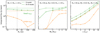 |
Fig. 8 Integrated fluxes of the methanol lines for models with low (green) and high (orange) mm opacity dust grains. The dashed lines show the envelope-only models, and the solid lines show the envelope-plus-disk models. The fiducial models are indicated by a cross. The models are the same as those plotted in Fig. 5. The dotted line indicates the minimum disk radius needed to see a drop of a factor of about two in intensity of the envelope-plus-disk model. |
3.3.3 Integrated Line Fluxes
Figure 8 presents the integrated fluxes of the continuum-subtracted methanol lines for the same models as Fig. 5 as a function of disk radius, envelope mass, and luminosity. The effect of the viewing angle is examined for the fiducial models. The two extreme cases of viewing angle, face-on and edge-on, show a difference smaller than a factor of two (Figs. E.7 and E.8). For the remainder of the paper, we therefore only present the values for the face-on view.
The trend shown in Fig. 5 as a function of envelope mass and luminosity is reflected in the integrated fluxes. However, the middle panel of Fig. 8 shows that the slope of the increase in methanol emission with the envelope mass decreases for envelope masses ≳ 3 M⊙. This is because the line becomes more optically thick (Fig. A.4). Moreover, the line fluxes increase with L. While we find that for the fiducial model the emission is always optically thick for the various luminosities (Fig. A.6), increasing the luminosity leads to an increase in the area of the emitting region because the snow line moves outwards, leading to an increase in the integrated flux.
Moreover, for the low mm opacity grains, the integrated fluxes stay constant as the disk radius increases, which is the same trend as observed for the warm methanol masses (Fig. 5, left panel), but for the high mm opacity grains, the fluxes decrease with increasing disk radius, which is the opposite of what is observed for the warm methanol masses. This difference can only be explained by the continuum over-subtraction effect discussed in Sect. 4.1. As explained in Sect. 3.2, a large part of the warm methanol mass comes from the disk component when the grains have a high mm opacity. Hence, if the gas in the disk is optically thick (Figs. A.3 and A.4) and the dust in the disk is optically thick as well (high mm opacity dust grains), the emission from the gas cannot be observed because the line is not brighter than the underlying continuum.
A comparison of the envelope-only models with high and low mm opacity dust grains (the two dashed lines) shows that there is a drop in integrated fluxes when the grains have a higher mm opacity. In addition to the lower warm methanol mass already described in Sect. 3.2, a radiative transfer effect that lowers the emission even further is dust attenuation in the envelope. The reason is that the large dust grains are more optically thick at millimetre wavelengths, and they therefore block the emission in the envelope.
For both low and high mm opacity grains, the envelope-only models have a higher integrated flux than the envelope-plus-disk models. This difference is more prominent when the grains have a high mm opacity. The only exception are models in which the envelope masses are 0.1 and 0.3 M⊙ and the grains have a high mm opacity. These trends are similar to what was shown in Fig. 5.
In the left panel of Fig. 8, in both low and high mm opacity dust models, the integrated line fluxes in the envelope-plus-disk models drop by a factor larger than ∼ 1.5–3 compared with the envelope-only models when the disk radius is at least 30 au. This disk radius would be smaller if the luminosity were lower, and it would be larger if the luminosity were higher. This is quite interesting as it could indicate a minimum disk size for sources with observed weak methanol emission compared with sources with a stronger methanol emission. We recall that RD is not the same as the observed gas or dust disk radii. Moreover, when κdust at mm is large, the drop in integrated fluxes between the envelope-only and envelope-plus-disk models increases to more than an order of magnitude for disks with radii larger than 50 au (Fig. 8 left panel). This drop for large disk sizes is much larger for high mm opacity dust grains than for low mm opacity dust grains because of the continuum over-subtraction in the optically thick dust disk that we discuss further in Sect. 4.1 (Fig. A.7).
3.4 Caveats
The abundances of methanol in the inner and outer envelope are parametrised with values matching the observations. However, the observed values vary by a factor of about three for low-mass young stellar objects ( ; Boogert et al. 2015; also see Bottinelli et al. 2010; Öberg et al. 2011). Moreover, Drozdovskaya et al. (2014) reported that the abundance of methanol gas and ice in the disk can change during the infall process. The values used in the disk were also parametrised and are on the lower side of those inspired by observations (Booth et al. 2021) and chemical modelling of Class II disks (Walsh et al. 2014). However, if these values are increased by an order of magnitude, the emission lines in the disk become more optically thick (Fig. A.5), but they still show values lower than the envelope-only models, as explained in Sect. 4.1. For example, if the methanol abundance in the disk component of the fiducial envelope-plus-disk model were increased by an order of magnitude, the integrated line flux would only be a factor of ∼1.04 times higher than that for the fiducial envelope-plus-disk model.
There are a number of assumptions in the physical structures of the models. We list the most important of them with explanation of their effects on the results of this work below.
Gas density structure: The gas density structure for the envelope-only model (Eq. (1)) and the envelope component of the envelope-plus-disk model (Eq. (2)) are not exactly the same. More precisely, at the inner radii, just above where the disk is located in the envelope-plus-disk model, the envelope-only model is denser than the envelope-plus-disk model. Therefore, part of the reason why the envelope-only models show more warm methanol mass is that these models have a higher density in the inner envelope. However, the difference between the densities in the inner envelope is at most a factor of five at radii of ∼20 au, and for most radii, it is below a factor of about five (see Fig. E.6). Hence, this cannot be the main reason why the envelope-only models have emission that is more than an order of magnitude stronger than the envelope-plus-disk models.
Shape of the outflow cavity: It has been assumed in the models that the outflow cavity has the same shape in the envelope-only and envelope-plus-disk models and is characterised by Eq. (3). Moreover, the outflow cavity opening angle and extent is the same in all the models. However, shape of the cavity at small scales and the mechanism that opens it is still debated and not fully understood. Furthermore, larger or smaller outflow cavities can affect the values reported in this work by enhancing or quenching the UV penetration depth (Drozdovskaya et al. 2015). Nevertheless, the main conclusion would stay the same: the envelope-plus-disk models show lower methanol emission due to the lower temperatures.
Disk scale height: The disk scale height is parametrised, and hence it is not self-consistent with the thermal structure of the disk. To examine the effect of disk scale height on the integrated line fluxes, the scale height was calculated using the mid-plane temperature of the fiducial model, and the fiducial model was run with the new consistent scale height. This resulted in an H/R of ∼0.06 at 1 au, compared with 0.2 used for the fiducial model. It is important to note that in reality, the mid-plane temperature refers to that of dust, whereas flaring depends on the gas temperatures, which decouples from those of dust in the surface layers. The gas temperature should be calculated self-consistently to obtain realistic structures. However, this calculation is computationally expensive and beyond the scope of this work, and we therefore used the mid-plane temperature. When the mid-plane temperature is used to determine the scale height, the integrated flux is only a factor ∼1.3 higher than what is assumed for the fiducial model. Therefore, its effect should not change the final conclusions of this work.
Disk extent: the disk was assumed to have a hard edge. The material beyond the disk edge is cold and thus does not contribute much to the methanol emission. Hence, adding a disk without a hard edge (e.g. an exponentially decaying density structure) will only change the amount of cold methanol in the models and does not affect the methanol fluxes significantly. Furthermore, the effect of a more extended disk on methanol emission is to decrease the emission in the envelope-plus-disk models because there will be a larger area in which the methanol abundance is 10–11 rather than 10–9. Therefore, the difference between the envelope-only model and the envelope-plus-disk models increase.
Free-fall velocity: no free-fall velocity was assumed in the models. Fiducial envelope-only and envelope-plus-disk models were run after adding free-fall velocity to the envelope component (the models are not shown here). The integrated flux for the envelope-only case is about twice higher and a factor of about 1.3 higher for the envelope-plus-disk case when free-fall velocity is added. This shows that adding free-fall velocity will only increase the difference between the envelope-only and the envelope-plus-disk models.
4 Discussion
4.1 Opacity Effects
In the previous section, we showed that the methanol emission from the envelope-plus-disk models is always lower than that of the envelope-only models. This is mainly due to the lower warm methanol mass in the envelope-plus-disk models as the temperatures are lower and hence the snow surfaces are closer to the central protostar.
The line optical depth effects can also become important. The fiducial model of envelope-plus-disk for the considered spectral line has optically thick methanol ( ) in the inner ∼50 au, and the fiducial envelope-only model has optically thick methanol between radii of ∼5 au and ∼60 au (Fig. A.3). Hence, the line flux in these regions is proportional to the emitting area, which is smaller in the envelope-plus-disk model because the snow surface lies closer to the protostar due to the presence of a disk and disk shadowing (Fig. 3). Therefore, a drop of a factor ∼3.5 in warm methanol mass has translated into a drop of a factor ∼1.5 in the integrated fluxes between the fiducial models of envelope-only and envelope-plus-disk. Furthermore, the line is more optically thick in the disk than in the envelope for the fiducial envelope-plus-disk model, especially in the inner 10 au. The line optical depth effects become especially strong when larger methanol abundances are assumed in the disk and the envelope. If the methanol abundance in the disk were higher by an order of magnitude for the fiducial envelope-plus-disk model, the envelope-only model would still have stronger methanol emission than the envelope-plus-disk model because the emitting area is smaller in the latter (see Fig. A.5).
As explained in Sect. 3.3.3, the drop in integrated fluxes is much larger between the two models when the dust grains have a high mm opacity. The temperature difference between the models with low and high mm opacity dust grains is small (Fig. 3). For example, the warm methanol mass is the same for the case of ME = 5 M⊙ between the envelope-only models with low and high mm opacity dust grains (Fig. 5), while there is a difference of a factor of about two between the integrated line fluxes of these two models. This points towards the effect of dust opacity rather than the temperature structure. The dust opacity has two types of effects: dust attenuation in the envelope, and continuum over-subtraction in the disk.
Dust attenuation in the envelope occurs on scales of ∼ 100 au in the envelope-only model. The dust with high mm opacity becomes marginally optically thick (≳0.1; see Fig. A.2) for envelope masses ≳1 M⊙. Together with the larger photodissociation regions, these are the main reasons for the drop in integrated fluxes between the two dashed lines in Fig. 8 (all panels). A cartoon of this effect is shown in Fig. 9, especially for the envelope components of the model (the two curved lines). This figure shows that the optically thick dust can be between the methanol emission in the envelope and the observer and thus blocks the methanol emission.
The continuum over-subtraction effect only occurs in the envelope-plus-disk model. This effect has been discussed in the literature (Boehler et al. 2017; Weaver et al. 2018; Rosotti et al. 2021) and states that continuum subtraction can cause an underestimation of the true line intensity if both the dust and the gas in front of the dust in the disk are optically thick and the line has a brightness similar to or lower than the underlying continuum. The total intensity at frequency v is the sum of the disk component intensity (Iv,D) and the envelope component intensity (Iv,E) and is given by
 (7)
(7)
where τ is the optical depth, Bv is the Planck function, and T is the temperature. Subscripts d and g denote dust and gas, and subscripts E and D denote the envelope and disk components, respectively. Here four layers of dust and gas are assumed, as shown schematically in Fig. 9.
This equation assumes that both the gas and dust in the disk and envelope have a finite optical depth. This means that in addition to the emission from each layer separately, the optically thick dust in the envelope absorbs some of the dust and gas emission behind it (the  terms), the optically thick gas in the envelope absorbs some of the dust and gas emission behind it (the
  terms), and the gas in the disk absorbs the dust emission behind it (the
  term). If the line and dust emission are optically thin, after the continuum subtraction (i.e. subtracting the first and fourth terms), Iv will be the true line intensity. However, if the dust and line emission are optically thick in the disk, the gas in the disk will absorb part of the dust emission (
 in the first term) and does not emerge over the continuum. Therefore, subtracting the dust intensity (first term) will eliminate some (or all) of the emission from the line in the disk.
This effect of the continuum over-subtraction is quantified in Fig. 10. This figure shows a cut through the image of the peak of the spectral line observed face-on for the envelope-plus-disk fiducial model with optically thick dust. Orange shows the cut through the image without continuum subtraction, blue shows the same after continuum subtraction, and green shows the same without dust in the calculation of the image. At radii smaller than ∼25 au, there is a difference of about an order of magnitude between the true line intensity (green) and the continuum-subtracted intensity (blue). This difference is smaller for radii between 25 au and 50 au, but it is still a factor of about four. However, there is no difference between the line only and the continuum-subtracted intensity where the disk stops (after 50 au). This figure shows that the continuum over-subtraction effect can lead to an error of a factor 4–10 in measuring the true line intensity.
To conclude, the dust can have three effects. It either blocks the emission in the envelope, or it hides the methanol emission and introduces an error when the emission is continuum subtracted. Moreover, the photodissociation regions are larger when high mm opacity dust grains are used because they are more optically thin to UV than low mm opacity dust grains.
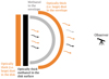 |
Fig. 9 Sketch of the emission from methanol and dust in the disk and envelope of the envelope-plus-disk model to emphasise the effects of dust optical depth on the disk and the envelope. In the envelope, the dust can block the methanol emission, whereas in the disk, the dust optical depth causes an error due to continuum over-subtraction although methanol is in front of the dust. |
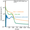 |
Fig. 10 Effect of continuum over-subtraction in the fiducial envelope-plus-disk model with large κdust at mm. Orange shows a radial cut through the methanol emission image including dust continuum at the line peak (0 km s–1). Green shows the same without dust in the model (true line intensity). Blue shows the same as orange but continuum subtracted. There is a difference of a factor of about four to up to an order of magnitude between the continuum-subtracted intensity and the true line intensity due to the continuum over-subtraction effect. |
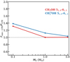 |
Fig. 11 Impact of non-LTE effect on the emission of the 51,4–41,3 transition of methanol (Eup = 49.7 K, Aij = 6.0 × 10⁻⁵) emitted from the inner 2″ of the envelope. The j-axis indicates the ratio of the integrated line flux computed with Ratran under non-LTE assumptions and LTE assumptions. The non-LTE computation was made with a consistent calculation of the population levels of methanol, including collision with H2 and radiative pumping. The line flux from |

4.2 Non-LTE Effects
Throughout this paper, the emission of methanol was computed under the LTE assumption. Critical densities of the low-lying methanol levels (Eup ≲ 100 K) are typically found to be about ncrit ≃ 106 cm–3 (Fig. C.1). It might therefore be expected that non-LTE effects might play a role in the low-density part of the envelope. In order to test the validity of our LTE approximation, we ran a series of non-LTE models using the Ratran modelling code (Hogerheijde & van der Tak 2000), taking collision with H2 (Rabli & Flower 2010) and radiative pumping into account. For the purpose of this work and in order to save computational time, the envelope was treated as a 1D spherically symmetric structure. The density follows the prescriptions detailed in Sect. 2.1.1, except that the outflow cavity was discarded. This provided a conservative estimation of the non-LTE effects because in the presence of a disk, methanol emission is confined to even denser regions, where LTE should be more appropriate. The thermal structure was computed with RADMC-3D, and the abundance of methanol was set as described in Sect. 2. For conciseness, only models with high mm opacity dust grains and L = 8 L⊙ were computed.
Figure 11 shows the ratio of the integrated line fluxes between two models, one computed with non-LTE assumptions, and the other with LTE assumptions as a function of envelope mass. Red shows this ratio for CH3OH and blue for  to consider the non-LTE effects on an optically thin line. It demonstrates that non-LTE effects do not significantly impact the intensity of the CH3OH 51,4–41,3 line (red) down to an envelope mass of 0.1 M⊙. The emission here is dominated by the region interior to the sublimation surface, which has densities above ∼ 107 cm–3. We note that Jørgensen et al. (2005) and Maret et al. (2005) performed full non-LTE calculations to model single-dish CH3OH emission, which was necessary in their case because their observed emission originated both from the hot core and from the larger-scale cold lower-density envelope.
Other than the high densities of the inner regions, the high opacity of the strong methanol line considered here also contributes to quenching the radiative de-excitation of the level, leading to LTE populations at densities even below the critical densities of the levels (photon trapping), which can help to explain the small difference between LTE and non-LTE models in Fig. 11. However, for the  51,4–41,3 line (blue), which is not affected by photon trapping (optically thin lines), the LTE assumption is largely valid because non-LTE calculations are only different by ∼20%. Interestingly, the non-LTE effect tends to enhance the line emission for this specific line. We also note that for more excited lines (Eup ≳ 300 K), non-LTE effects start to be important. This was confirmed by studying the population of an excited level, which substantially deviated from LTE.
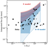 |
Fig. 12 Comparison of the integrated intensities found from the models with observations (black circles) normalised to a source distance of 150 pc. Red represents the regions with envelope-only models, and blue shows the regions with envelope-plus-disk models. The smooth regions indicate the models with low mm opacity dust grains, and striped regions show the models with high mm opacity dust grains. The envelope-only models with high mm opacity dust grains and envelope masses of 0.1 M⊙ and 0.3 M⊙ are not included here as most of the envelope is photodissociated (Sect. 3.2). Triangles show the upper limits found from observations, and the hollow points are sources with a disk. To explain most of the data, both a disk and optically thick dust are needed. |
4.3 Comparison with Observations
We now address the main question of this paper, that is, whether the source structure can explain the lack of methanol emission that is observed for some sources. Figure 12 shows integrated fluxes of the CH3OH 51,4–41,3 transition at 243.916 GHz from the PEACHES survey (Yang et al. 2021; van Gelder et al. 2022) in black with the envelope-only models in red and envelope-plus-disk models in blue. The smooth coloured regions show where models with low mm opacity dust fall, and the striped regions show the same for models with large mm opacity dust.
The envelope-only models cannot explain the bulk of the observations for the adopted methanol abundances. They can only explain the observations with high methanol fluxes, but cannot explain the sources with low methanol emission even when the dust is highly optically thick. This is important because it shows that thinking about protostars as envelope-only objects is not necessarily correct. The CH3OH abundance would have to be up to two orders of magnitude lower to explain the range. This is inconsistent with ice observations of dense clouds assuming that all the ices sublimate inside the snow surface without subsequent chemistry.
The envelope-plus-disk models, however, can explain most of the observations because they have lower integrated line fluxes. A group of sources with very low methanol emission can only be reproduced by models with disk and high mm opacity dust grains (high dust optical depths). Therefore, to understand the observations, the disk and the dust optical depth effects need to be taken into account, that is, dust grains with large κdust at mm.
Based on the results from this work, we can conclude that most of the sources without strong CH3OH emission that are observed as part of the PEACHES survey (Yang et al. 2021) are prime targets for finding disks in low-mass protostars. To test this hypothesis, cold species such as DCO+ can be studied (as done by Murillo et al. 2018) in the protostars observed by the PEACHES survey. Moreover, observations of these sources at longer wavelengths (as done by De Simone et al. 2020 for NGC 1333 IRAS 4A1) can help distinguish between the non-existence of complex organics in a source and the dust optical depth effects in the disk and the envelope. Furthermore, very high angular resolution observations (∼30 au) can help resolve very small disks in the continuum.
The hollow markers in Fig. 12 indicate the sources that are confirmed to have a disk from the VLA Nascent Disk and Multiplicity (VANDAM) survey (Segura-Cox et al. 2018). It is reassuring that all cannot be explained by the envelope-only models. In other examples in the literature, sources with disks show no or a lower emission of complex organic molecules. For example, Tychoniec et al. (2021) observed a large resolved dust structure in the Class 0 source Serpens SMM3, perpendicular to the outflow that might be a disk, but failed to find strong emission of methanol or complex species towards this source, despite the high luminosity of the source (Lbol ≃ 28 L⊙). Artur de la Villarmois et al. (2019) found no methanol emission towards 12 Class I protostars hosting disks that they observed in the Ophiuchus molecular cloud. Moreover, van ’t Hoff et al. (2020) did not detect methanol towards the two young disks L1527 IRS and IRAS 04302+2247 (also see Podio et al. 2020). In addition, Lee et al. (2017, Lee et al. 2019) reported that the presence of a disk can affect the emission from complex organic molecules in HH212.
Alternative explanations for the large spread may exist. We did not model the CH3OH chemistry explicitly, but used parametrised abundances inspired by observations and detailed gas-grain chemistry models. Notsu et al. (2021) studied the effect of X-rays on molecular abundances in the inner warm envelope, most notably, H2O and CH3OH. Some low-mass Class 0 sources are known to be strong X-ray emitters (e.g. Forbrich et al. 2006; Grosso et al. 2020), and for high X-ray luminosities, LX ≳ 1030 erg s–1, gaseous H2O and CH3OH are efficiently destroyed within their snow lines. This could result in low CH3OH line intensities for some of our sources. X-ray destruction can be distinguished from the scenarios discussed here through observations of HCO+ and its optically thin H13CO+ isotopologue (see also van ’t Hoff et al. 2021): if X-ray destruction dominates, HCO+ emission would be centrally peaked on source, having a high abundance even within the water snow line because its main destroyer (water) is absent. Notsu et al. (2021), see their Section 4.6, identified two sources in the Perseus Class 0 sample with weak CH3OH emission and centrally peaked HCO+ for which this could be the case. Additional deep surveys of both CH3OH and H13CO+ of this sample are needed to assess how common this explanation is.
5 Conclusions
This work investigated whether the presence of disks can explain the lack of methanol emission from some low-mass protostellar systems. Two models were considered: a spherically symmetric envelope-only model with an outflow cavity, and a flattened envelope model with an embedded disk and an outflow cavity. Radiative transfer calculations were performed for these two models using the radiative transfer code RADMC-3D to calculate the thermal structure and next, methanol emission assuming parametrised abundances and LTE excitation. The main conclusions of this work are summarised below.
The envelope-plus-disk models always show lower methanol emission than the envelope-only models. This is mainly due to disk shadowing and lower temperatures in the disk mid-plane. These two effects result in smaller sublimation regions, and hence, in a lower warm methanol mass in the envelope-plus-disk model.
The methanol emission from the envelope-plus-disk model is weaker than the envelope-only models by a factor of about two if the disk is at least 30 au in size (for L = 8 L⊙).
The drop in intensities between the two models increases by more than one order of magnitude when dust grains have a high mm opacity and the disk is at least 50 au in size (for L = 8 L⊙). This is because of the continuum over-subtraction in the disk.
The models can only explain the observations (spread of about two orders of magnitude in line intensities) if both disk shadowing and dust optical depth effects (i.e. dust attenuation in the envelope, continuum over-subtraction in the disk, and larger photodissociation regions) are taken into account (see Fig. 12). Considering only one of these effects is not enough to explain the data.
We suggest that most of the objects observed by the PEACHES survey may be hosting a disk, and those without strong CH3OH emission are prime targets for a search for disks in the embedded phase of star formation.
The presence of a disk along with dust optical depth effects can explain the lack of emission in some protostars. Hence, less methanol or complex organic molecule emission does not necessarily imply absence of these molecules or reprocessing of them in the gas phase. This work shows that to understand the chemistry of protostellar systems, the physical structure should be taken into account. In particular, protostars are not necessarily envelope-only objects, and the presence of a disk already has an effect on the molecular emission even in the earliest phases of star formation.
Acknowledgements
We would like to thank the referee for very useful comments. We would like to thank Jes K. Jørgensen and John H. Black for helpful discussions. Astrochemistry in Leiden is supported by the Netherlands Research School for Astronomy (NOVA), by funding from the European Research Council (ERC) under the European Union’s Horizon 2020 research and innovation programme (grant agreement No. 101019751 MOLDISK), and by the Dutch Research Council (NWO) grants 648.000.022, 618.000.001 and TOP-1 614.001.751. Support by the Danish National Research Foundation through the Center of Excellence “Inter-Cat” (Grant agreement no.: DNRF150) is also acknowledged. G.R. acknowledges support from the Netherlands Organisation for Scientific Research (NWO, program number 016.Veni.192.233) and from an STFC Ernest Rutherford Fellowship (grant number ST/T003855/1).
Appendix A Optical Depth
Figure A.1 shows the optical properties of the two dust distributions. The top panel shows the dust absorption opacity, and the bottom panel shows the albedo. Figure A.2 shows the dust optical depth for the fiducial envelope-only models with different envelope masses and high mm opacity dust grains.
Figure A.3 shows the line optical depth for the fiducial models. The blue line in this figure is τ when the disk methanol abundance is set to zero, so it shows τ in the envelope component of the fiducial envelope-plus-disk model. Figure A.4 shows line optical depth as a function of radius for fiducial models with an envelope mass of 3 M⊙ and the fiducial model with disk radius of 200 au. Figure A.5 shows the line optical depth versus radius for the fiducial envelope-plus-disk model and the same with one order of magnitude higher methanol abundance in its disk component. Figure A.6 shows the peak line optical depth of a radial cut for the fiducial models with different luminosities.
Figure A.7 shows the effect of continuum over-subtraction for the fiducial envelope-plus-disk model with high mm opacity dust grains and disk radius of 200 au.
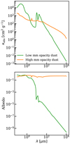 |
Fig. A.1 Properties of the dust grains. Albedo is defined as the scattering opacity divided by the sum of the absorption and scattering opacities. |
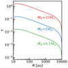 |
Fig. A.2 Radial cut of the dust optical depth for the fiducial model with high mm opacity dust in the envelope-only model with different envelope masses. The envelope becomes marginally optically thick in the inner ∼100 au for envelope masses above 1 M⊙. |
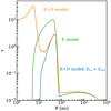 |
Fig. A.3 Radial cut through the line optical depth for the fiducial models (small κdust at mm). Orange and green show τ for the envelope-plus-disk and envelope-only fiducial models. Blue shows τ for the envelope component of the envelope-plus-disk model where the model is run by setting the methanol abundance to zero in the disk. The line is more optically thick in the disk than in the envelope. |
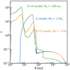 |
Fig. A.4 Radial cut through the line optical depth for fiducial models with an envelope mass of 3 M⊙ and fiducial models with a disk radius of 200 au. |
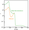 |
Fig. A.5 Radial cut through the line optical depth of the image at the peak of the line for fiducial envelope-plus-disk model and the same with a disk methanol abundance higher by one order of magnitude. |
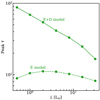 |
Fig. A.6 Peak line optical depth of a radial cut for fiducial models with various luminosities. |
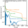 |
Fig. A.7 Same as Fig. 10, but for the fiducial model with a disk radius of 200 au and high mm opacity dust grains. |
Appendix B Abundance of Methanol
In Eq. (6) we need to find the average of  . Moreover, nd can be written in terms of the average of
  . The average of
  and
and  can be written as
 (B.1)
(B.1)

respectively. Here β depends on the dust distribution, and amin and amax are the minimum and maximum dust grain sizes in a dust distribution, respectively. We assumed β to be 3.5 for the large dust grain distribution (high mm opacity dust). The average of  for the high mm opacity dust distribution in this work is 1.25 × 10⁻¹⁰ mm2 so that
  .
.
Therefore, using Eqs. (B.1) and (B.2), the expression  can be written in terms of hydrogen number density (nH), dust-to-gas mass ratio (Q) dust grains bulk density (ρd), minimum and maximum dust grain sizes as
 (B.3)
(B.3)
Here mp is the proton mass, and the factor 1.4 takes the helium mass into account. Hence, for the small silicate dust grains used in this work, where all the dust grains have a size of 0.1 μm and ρd = 3.7g cm–3, the dust number density would be 1.5×10⁻¹²nH.
Appendix C Critical Density
Figure C.1 shows the critical density of the methanol line studied here as a function of temperature. The critical density is defined as the density above which the collisional de-excitation of a specific level equals the radiative de-excitation of that level. With this definition, we can conveniently estimate whether the energy levels are populated according to a Boltzmann distribution. It is weakly dependent on temperature and computed for a particular level using the following equation (Draine 2011):
 (C.1)
(C.1)
Here Au,1 is the Einstein A coefficient for a transition with upper and lower levels u and 1, respectively, and Ku,1 is the collision rate coefficient for that transition. The energy levels and Einstein A coefficients for the line studied in this work were taken from the Cologne Database for Molecular Spectroscopy (CDMS) (Müller et al. 2001, Müller et al. 2005; Xu et al. 2008), and the collisional rate coefficients were taken from Rabli & Flower (2010).
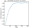 |
Fig. C.1 Critical density for the methanol line. The variation in critical density in this plot is less than a factor of two. |
Appendix D Model Grid
Figure D.1 shows the effects of various parameters of the disk and the envelope on the temperature structure.
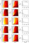 |
Fig. D.1 Two-dimensional dust temperatures in the envelope-only models (left column) and in the envelope-plus-disk models (middle column). The white contours show the location in which the temperature is 70 K as an indication of the approximate temperature at which methanol is sublimated at the densities of the models using the gas-grain balance model. The right column shows the comparison of the mid-plane temperature in the envelope-plus-disk models and the envelope-only models. The rows from top to bottom present the fiducial model, the fiducial model when the dust grains have a high mm opacity, the fiducial model with a stellar luminosity of 32 L⊙, the fiducial model when the envelope mass is 5 M⊙, and the fiducial model with a disk radius of 20 au. |
Appendix E Additional Plots
Figure E.1 shows the warm methanol mass for the disk component and the envelope component of the fiducial envelope-plus-disk model in blue and the same for the fiducial envelope-only model in red. This figure shows that the warm methanol mass is dominated by the envelope component of the envelope-plus-disk model. Figure E.2 shows the warm methanol mass in the disk and envelope components of the envelope-plus-disk models. Blue shows the fiducial model with a high mm opacity dust grains and a disk radius of 200 au for various luminosities, and orange shows the fiducial model with high mm opacity dust grains for various luminosities. There is more warm methanol mass in the disk component when the disk radius is 200 au than when the disk radius is 50 au. Moreover, for most luminosities shown here, the warm mass is dominated by the disk component rather than the envelope component, which is the opposite of the case of the fiducial model (low mm opacity dust grains, Figure E.1). This is because the larger photodissociation regions dominate the envelope component when the grains have a high mm opacity (Fig. 4 and E.5).
Figure E.3 shows methanol abundance maps for fiducial models with an envelope mass of 5 M⊙. Figure E.4 and E.5 show methanol abundance maps for the fiducial envelope-plus-disk models with various disk radii for low and high mm opacity dust grains, respectively.
Figure E.6 shows a cut through the density of total H for the fiducial envelope-only and envelope-plus-disk models to examine the difference between the density in the envelope component of the two models. Figure E.7 shows the effect of viewing angle on the integrated line fluxes for the fiducial models with low and high mm opacity dust grains. Figure E.8 is the same as E.7, but for models with an envelope mass of 5 M⊙.
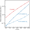 |
Fig. E.1 Disk and envelope components of warm mass for the fiducial models with various luminosities. Red shows the envelope-only model, and blue shows the envelope-plus-disk model. The solid line shows the envelope-component (i.e. Ein) of warm mass in the envelope-plus-disk model, and the dashed line shows this for the disk component (i.e. Din). |
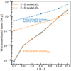 |
Fig. E.2 Comparison between disk and envelope components of the fiducial model with high mm opacity dust grains and various luminosities (orange) and the same when disk radius is 200 au. The solid line shows the envelope-component (i.e. Ein) of warm mass in the envelope-plus-disk model, and the dashed line shows this for the disk component (i.e. Din). |
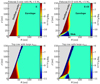 |
Fig. E.3 Methanol abundance maps for the envelope-only (left) and envelope-plus-disk (right) models when the envelope mass is 5 M⊙ and the other parameters are the same as the fiducial model. The top row shows the models with low mm opacity grains, and the bottom row shows the models with high mm opacity grains. The photodissociation regions for ME = 5 M⊙ models are very small, and they are similar in models with low and high mm opacity grains, which is different from the fiducial model in Fig. 4. |
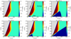 |
Fig. E.4 Methanol abundance maps for the fiducial envelope-plus-disk models with low mm opacity dust grains and different disk radii. |
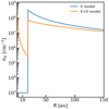 |
Fig. E.6 Cut through the densities of the fiducial envelope-only and envelope-plus-disk model. The cut is in a direction just above where the disk is located to compare the densities in the envelope-only model and the envelope component of the envelope-plus-disk model. |
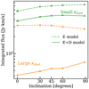 |
Fig. E.7 Effect of viewing angle on the integrated line fluxes for the fiducial models. |
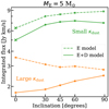 |
Fig. E.8 Effect of viewing angle on the integrated line fluxes for the fiducial models with an envelope mass of 5 M⊙. |
References
- Aikawa, Y., Furuya, K., Yamamoto, S., & Sakai, N. 2020, ApJ, 897, 110 [Google Scholar]
- Artur de la Villarmois, E., Jørgensen, J.K., Kristensen, L.E., et al. 2019, A&A, 626, A71 [NASA ADS] [CrossRef] [EDP Sciences] [Google Scholar]
- Bachiller, R., & Tafalla, M. 1999, in NATO Advanced Study Institute (ASI) Series C, 540, The Origin of Stars and Planetary Systems, eds. C.J. Lada, & N.D. Kylafis, 227 [CrossRef] [Google Scholar]
- Belloche, A., Müller, H. S. P., Menten, K. M., Schilke, P., & Comito, C. 2013, A&A, 559, A47 [NASA ADS] [CrossRef] [EDP Sciences] [Google Scholar]
- Belloche, A., Maury, A. J., Maret, S., et al. 2020, A&A, 635, A198 [NASA ADS] [CrossRef] [EDP Sciences] [Google Scholar]
- Bisschop, S. E., Jørgensen, J.K., van Dishoeck, E.F., & de Wachter, E.B.M. 2007, A&A, 465, 913 [NASA ADS] [CrossRef] [EDP Sciences] [Google Scholar]
- Blake, G. A., Sutton, E. C., Masson, C. R., & Phillips, T. G. 1987, ApJ, 315, 621 [Google Scholar]
- Boehler, Y., Weaver, E., Isella, A., et al. 2017, ApJ, 840, 60 [Google Scholar]
- Bøgelund, E.G., McGuire, B.A., Ligterink, N.F.W., et al. 2018, A&A, 615, A88 [NASA ADS] [CrossRef] [EDP Sciences] [Google Scholar]
- Boogert, A. C. A., Pontoppidan, K. M., Knez, C., et al. 2008, ApJ, 678, 985 [Google Scholar]
- Boogert, A. C. A., Huard, T.L., Cook, A.M., et al. 2011, ApJ, 729, 92 [NASA ADS] [CrossRef] [Google Scholar]
- Boogert, A. C. A., Gerakines, P. A., & Whittet, D. C. B. 2015, ARA&A, 53, 541 [Google Scholar]
- Booth, A. S., Walsh, C., Terwisscha van Scheltinga, J., et al. 2021, Nat. Astron., 5, 684 [NASA ADS] [CrossRef] [Google Scholar]
- Bottinelli, S., Boogert, A. C. A., Bouwman, J., et al. 2010, ApJ, 718, 1100 [NASA ADS] [CrossRef] [Google Scholar]
- Caselli, P., & Ceccarelli, C. 2012, A&Ar, 20, 56 [NASA ADS] [CrossRef] [Google Scholar]
- Chiang, E. I., & Goldreich, P. 1997, ApJ, 490, 368 [Google Scholar]
- Crapsi, A., van Dishoeck, E. F., Hogerheijde, M. R., Pontoppidan, K. M., & Dullemond, C. P. 2008, A&A, 486, 245 [NASA ADS] [CrossRef] [EDP Sciences] [Google Scholar]
- Dartois, E., Schutte, W., Geballe, T. R., et al. 1999, A&A, 342, L32 [NASA ADS] [Google Scholar]
- Dartois, E., d’Hendecourt, L., Thi, W., Pontoppidan, K.M., & van Dishoeck, E.F. 2002, A&A, 394, 1057 [NASA ADS] [CrossRef] [EDP Sciences] [Google Scholar]
- De Simone, M., Ceccarelli, C., Codella, C., et al. 2020, ApJ, 896, L3 [NASA ADS] [CrossRef] [Google Scholar]
- Draine, B. T. 2011, Physics of the Interstellar and Intergalactic Medium [Google Scholar]
- Drozdovskaya, M. N., Walsh, C., Visser, R., Harsono, D., & van Dishoeck, E. F. 2014, MNRAS, 445, 913 [NASA ADS] [CrossRef] [Google Scholar]
- Drozdovskaya, M. N., Walsh, C., Visser, R., Harsono, D., & van Dishoeck, E. F. 2015, MNRAS, 451, 3836 [NASA ADS] [CrossRef] [Google Scholar]
- Dullemond, C. P., Dominik, C., & Natta, A. 2001, ApJ, 560, 957 [NASA ADS] [CrossRef] [Google Scholar]
- Forbrich, J., Preibisch, T., & Menten, K. M. 2006, A&A, 446, 155 [NASA ADS] [CrossRef] [EDP Sciences] [Google Scholar]
- Fuchs, G. W., Cuppen, H. M., Ioppolo, S., et al. 2009, A&A, 505, 629 [NASA ADS] [CrossRef] [EDP Sciences] [Google Scholar]
- Garrod, R. T., & Pauly, T. 2011, ApJ, 735, 15 [Google Scholar]
- Gavino, S., Dutrey, A., Wakelam, V., et al. 2021, A&A, 654, A65 [NASA ADS] [CrossRef] [EDP Sciences] [Google Scholar]
- Geballe, T. R., Kim, Y. H., Knacke, R. F., & Noll, K. S. 1988, ApJ, 326, L65 [NASA ADS] [CrossRef] [Google Scholar]
- Geppert, W. D., Hamberg, M., Thomas, R. D., et al. 2006, Faraday Discuss., 133, 177 [Google Scholar]
- Gibb, E., Nummelin, A., Irvine, W. M., Whittet, D. C. B., & Bergman, P. 2000, ApJ, 545, 309 [NASA ADS] [CrossRef] [Google Scholar]
- Grosso, N., Hamaguchi, K., Principe, D. A., & Kastner, J. H. 2020, A&A, 638, A4 [NASA ADS] [CrossRef] [EDP Sciences] [Google Scholar]
- Harsono, D., Bruderer, S., & van Dishoeck, E. F. 2015, A&A, 582, A41 [NASA ADS] [CrossRef] [EDP Sciences] [Google Scholar]
- Hasegawa, T. I., Herbst, E., & Leung, C. M. 1992, ApJS, 82, 167 [Google Scholar]
- Heays, A. N., Bosman, A. D., & van Dishoeck, E. F. 2017, A&A, 602, A105 [NASA ADS] [CrossRef] [EDP Sciences] [Google Scholar]
- Herbst, E., & van Dishoeck, E. F. 2009, ARA&A, 47, 427 [NASA ADS] [CrossRef] [Google Scholar]
- Hidaka, H., Watanabe, N., Shiraki, T., Nagaoka, A., & Kouchi, A. 2004, ApJ, 614, 1124 [Google Scholar]
- Hogerheijde, M. R., & van der Tak, F.F.S. 2000, A&A, 362, 697 [NASA ADS] [Google Scholar]
- Ilee, J. D., Cyganowski, C. J., Nazari, P., et al. 2016, MNRAS, 462, 4386 [NASA ADS] [CrossRef] [Google Scholar]
- Jørgensen, J. K., Schöier, F. L., & van Dishoeck, E. F. 2002, A&A, 389, 908 [CrossRef] [EDP Sciences] [Google Scholar]
- Jørgensen, J. K., Schöier, F. L., & van Dishoeck, E. F. 2005, A&A, 437, 501 [NASA ADS] [CrossRef] [EDP Sciences] [Google Scholar]
- Jørgensen, J. K., van Dishoeck, E. F., Visser, R., et al. 2009, A&A, 507, 861 [NASA ADS] [CrossRef] [EDP Sciences] [Google Scholar]
- Jørgensen, J. K., van der Wiel, M.H.D., Coutens, A., et al. 2016, A&A, 595, A117 [NASA ADS] [CrossRef] [EDP Sciences] [Google Scholar]
- Kristensen, L. E., van Dishoeck, E. F., Bergin, E. A., et al. 2012, A&A, 542, A8 [NASA ADS] [CrossRef] [EDP Sciences] [Google Scholar]
- Laas, J. C., Garrod, R. T., Herbst, E., & Widicus Weaver, S. L. 2011, ApJ, 728, 71 [Google Scholar]
- Law, C. J., Zhang, Q., Öberg, K. I., et al. 2021, ApJ, 909, 214 [Google Scholar]
- Lee, C.-F., Li, Z.-Y., Ho, P. T. P., et al. 2017, ApJ, 843, 27 [NASA ADS] [CrossRef] [Google Scholar]
- Lee, C.-F., Codella, C., Li, Z.-Y., & Liu, S.-Y. 2019, ApJ, 876, 63 [Google Scholar]
- Ligterink, N. F. W., Ahmadi, A., Coutens, A., et al. 2021, A&A, 647, A87 [NASA ADS] [CrossRef] [EDP Sciences] [Google Scholar]
- López-Sepulcre, A., Sakai, N., Neri, R., et al. 2017, A&A, 606, A121 [NASA ADS] [CrossRef] [EDP Sciences] [Google Scholar]
- Manigand, S., Jørgensen, J. K., Calcutt, H., et al. 2020, A&A, 635, A48 [NASA ADS] [CrossRef] [EDP Sciences] [Google Scholar]
- Marcelino, N., Gerin, M., Cernicharo, J., et al. 2018, A&A, 620, A80 [NASA ADS] [CrossRef] [EDP Sciences] [Google Scholar]
- Maret, S., Ceccarelli, C., Caux, E., et al. 2004, A&A, 416, 577 [NASA ADS] [CrossRef] [EDP Sciences] [Google Scholar]
- Maret, S., Ceccarelli, C., Tielens, A. G. G. M., et al. 2005, A&A, 442, 527 [NASA ADS] [CrossRef] [EDP Sciences] [Google Scholar]
- Martin-Doménech, R., Bergner, J. B., Öberg, K. I., & Jørgensen, J. K. 2019, ApJ, 880, 130 [CrossRef] [Google Scholar]
- Maury, A. J., André, P., Testi, L., et al. 2019, A&A, 621, A76 [NASA ADS] [CrossRef] [EDP Sciences] [Google Scholar]
- McGuire, B. A., Shingledecker, C. N., Willis, E. R., et al. 2017, ApJ, 851, L46 [Google Scholar]
- Mottram, J. C., van Dishoeck, E. F., Kristensen, L. E., et al. 2017, A&A, 600, A99 [NASA ADS] [CrossRef] [EDP Sciences] [Google Scholar]
- Müller, H. S. P., Thorwirth, S., Roth, D. A., & Winnewisser, G. 2001, A&A, 370, L49 [Google Scholar]
- Müller, H. S. P., Schlöder, F., Stutzki, J., & Winnewisser, G. 2005, J. Mol. Struct., 742, 215 [Google Scholar]
- Murillo, N. M., Lai, S.-P., Bruderer, S., Harsono, D., & van Dishoeck, E. F. 2013, A&A, 560, A103 [NASA ADS] [CrossRef] [EDP Sciences] [Google Scholar]
- Murillo, N. M., Bruderer, S., van Dishoeck, E. F., et al. 2015, A&A, 579, A114 [NASA ADS] [CrossRef] [EDP Sciences] [Google Scholar]
- Murillo, N. M., van Dishoeck, E. F., van der Wiel, M.H.D., et al. 2018, A&A, 617, A120 [NASA ADS] [CrossRef] [EDP Sciences] [Google Scholar]
- Nazari, P., van Gelder, M. L., van Dishoeck, E. F., et al. 2021, A&A, 650, A150 [EDP Sciences] [Google Scholar]
- Notsu, S., van Dishoeck, E. F., Walsh, C., Bosman, A. D., & Nomura, H. 2021, A&A, 650, A180 [NASA ADS] [CrossRef] [EDP Sciences] [Google Scholar]
- Nourry, S., & Krim, L. 2015, MNRAS, 452, 3319 [NASA ADS] [CrossRef] [Google Scholar]
- Öberg, K. I., Boogert, A. C. A., Pontoppidan, K. M., et al. 2011, ApJ, 740, 109 [Google Scholar]
- Penteado, E. M., Walsh, C., & Cuppen, H. M. 2017, ApJ, 844, 71 [Google Scholar]
- Persson, M. V., Jørgensen, J. K., & van Dishoeck, E. F. 2012, A&A, 541, A39 [NASA ADS] [CrossRef] [EDP Sciences] [Google Scholar]
- Persson, M. V., Harsono, D., Tobin, J. J., et al. 2016, A&A, 590, A33 [NASA ADS] [CrossRef] [EDP Sciences] [Google Scholar]
- Plunkett, A. L., Arce, H. G., Corder, S. A., et al. 2013, ApJ, 774, 22 [NASA ADS] [CrossRef] [Google Scholar]
- Podio, L., Garufi, A., Codella, C., et al. 2020, A&A, 642, L7 [NASA ADS] [CrossRef] [EDP Sciences] [Google Scholar]
- Pringle, J. E. 1981, ARA&A, 19, 137 [NASA ADS] [CrossRef] [Google Scholar]
- Qasim, D. 2020, PhD Thesis [Google Scholar]
- Rabli, D., & Flower, D. R. 2010, MNRAS, 406, 95 [Google Scholar]
- Rosotti, G. P., Ilee, J. D., Facchini, S., et al. 2021, MNRAS, 501, 3427 [Google Scholar]
- Sanhueza, P., Jackson, J. M., Foster, J. B., et al. 2013, ApJ, 773, 123 [NASA ADS] [CrossRef] [Google Scholar]
- Schöier, F. L., van der Tak, F.F.S., van Dishoeck, E.F., & Black, J.H. 2005, A&A, 432, 369 [NASA ADS] [CrossRef] [EDP Sciences] [Google Scholar]
- Scibelli, S., Shirley, Y., Vasyunin, A., & Launhardt, R. 2021, MNRAS, 504, 5754 [NASA ADS] [CrossRef] [Google Scholar]
- Segura-Cox, D. M., Looney, L. W., Tobin, J. J., et al. 2018, ApJ, 866, 161 [Google Scholar]
- Shakura, N. I., & Sunyaev, R. A. 1973, A&A, 500, 33 [NASA ADS] [Google Scholar]
- Tabone, B., van Hemert, M. C., van Dishoeck, E. F., & Black, J. H. 2021, A&A, 650, A192 [NASA ADS] [CrossRef] [EDP Sciences] [Google Scholar]
- Taquet, V., Bianchi, E., Codella, C., et al. 2019, A&A, 632, A19 [NASA ADS] [CrossRef] [EDP Sciences] [Google Scholar]
- Tobin, J. J., Sheehan, P. D., Megeath, S. T., et al. 2020, ApJ, 890, 130 [CrossRef] [Google Scholar]
- Tychoniec, E., van Dishoeck, E. F., van’t Hoff, M.L.R., et al. 2021, A&A, 655, A65 [NASA ADS] [CrossRef] [EDP Sciences] [Google Scholar]
- Ulrich, R. K. 1976, ApJ, 210, 377 [Google Scholar]
- van Dishoeck, E. F., Blake, G. A., Jansen, D. J., & Groesbeck, T. D. 1995, ApJ, 447, 760 [Google Scholar]
- van Dishoeck, E. F., Kristensen, L. E., Mottram, J. C., et al. 2021, A&A, 648, A24 [NASA ADS] [CrossRef] [EDP Sciences] [Google Scholar]
- van Gelder, M. L., Tabone, B., Tychoniec, L., et al. 2020, A&A, 639, A87 [NASA ADS] [CrossRef] [EDP Sciences] [Google Scholar]
- van Gelder, M. L., Nazari, P., Tabone, B., et al. 2022, A&A, 662, A67 [NASA ADS] [CrossRef] [EDP Sciences] [Google Scholar]
- van Kempen, T. A., van Dishoeck, E. F., Güsten, R., et al. 2009, A&A, 501, 633 [NASA ADS] [CrossRef] [EDP Sciences] [Google Scholar]
- van ’t Hoff, M.L.R., Harsono, D., Tobin, J.J., et al. 2020, ApJ, 901, 166 [CrossRef] [Google Scholar]
- van’t Hoff, M.L.R., Harsono, D., van Gelder, M.L., et al. 2021, ApJ, accepted [arXiv:2110.08286] [Google Scholar]
- Visser, R., Doty, S. D., & van Dishoeck, E. F. 2011, A&A, 534, A132 [NASA ADS] [CrossRef] [EDP Sciences] [Google Scholar]
- Visser, R., Jørgensen, J. K., Kristensen, L. E., van Dishoeck, E. F., & Bergin, E. A. 2013, ApJ, 769, 19 [NASA ADS] [CrossRef] [Google Scholar]
- Walsh, C., Millar, T. J., Nomura, H., et al. 2014, A&A, 563, A33 [NASA ADS] [CrossRef] [EDP Sciences] [Google Scholar]
- Weaver, E., Isella, A., & Boehler, Y. 2018, ApJ, 853, 113 [Google Scholar]
- Whitney, B. A., Wood, K., Bjorkman, J. E., & Wolff, M. J. 2003, ApJ, 591, 1049 [Google Scholar]
- Xu, L.-H., Fisher, J., Lees, R. M., et al. 2008, J. Mol. Spectrosc., 251, 305 [NASA ADS] [CrossRef] [Google Scholar]
- Yang, Y.-L., Evans, Neal J.I., Smith, A., et al. 2020, ApJ, 891, 61 [CrossRef] [Google Scholar]
- Yang, Y.-L., Sakai, N., Zhang, Y., et al. 2021, ApJ, 910, 20 [Google Scholar]
- Ysard, N., Koehler, M., Jimenez-Serra, I., Jones, A. P., & Verstraete, L. 2019, A&A, 631, A88 [NASA ADS] [CrossRef] [EDP Sciences] [Google Scholar]
All Tables
All Figures
|
Fig. 1 Density profiles explored in this work. Left panel: 2D hydrogen nucleus number density, nH = n(H) + 2n(H2), for the fiducial envelope-only model. Right panel: Same as left panel, but for the fiducial flattened envelope-plus-disk model. In this figure and throughout, log is in base 10. |
| In the text | |
|
Fig. 2 Cartoon of the physical structure of the envelope-plus-disk model. H(R) and RD are the disk scale height and the disk radius. Din and Dout are the inner and outer part of the disk with respect to the sublimation surface. Ein and Eout are the same, but for the envelope. |
| In the text | |
|
Fig. 3 Two-dimensional dust temperatures in the envelope-only models (left column) and in the envelope-plus-disk models (middle column). The white contours show the location in which the temperature is 70 K as an indication of the approximate temperature at which methanol is sublimated at the densities of the models. The right column compares the mid-plane temperature in the envelope-plus-disk models and the envelope-only models. The first row presents the fiducial model, and the second row presents the fiducial model with high mm opacity dust grains. In all figures in this work, κdust refers to the opacity of the dust grains at mm wavelengths. On average, the temperatures are lower when a disk is present and when grains have high mm opacity. |
| In the text | |
|
Fig. 4 Methanol abundance maps for the envelope-only (left) and envelope-plus-disk (right) models. The magenta contours show where the temperature is 70 K to indicate where the approximate sublimation surfaces of methanol are at the densities in the models. The photodissociation region (τUV < 3) is much larger in the envelope for the dust distribution with high mm opacity. |
| In the text | |
|
Fig. 5 Change in warm methanol mass with disk radius (left panel), envelope mass (middle panel), and luminosity (right panel). The dashed lines show the envelope-only models, and the solid lines show the envelope-plus-disk models. The fiducial models are indicated by a cross. The warm methanol mass is computed inside the methanol snow surface where the methanol abundance is higher than 10–9 in the envelope and higher than 10–11 in the disk (i.e. the methanol mass in Din and Ein in Fig. 2) for models with low mm opacity dust grains (green) and high mm opacity dust grains (orange). In the models in which RD is varied, luminosity and mass of the envelope are fixed to 8 L⊙ and 1 M⊙. The dashed lines are constant in the left panel because the envelope-only models do not have a disk for which its radius can be altered. Where ME is varied, the luminosity, disk mass, and radius are fixed to 8 L⊙, 0.01 M⊙, and 50 au. Where the luminosity is varied, the envelope mass, disk mass, and radius are fixed to 1 M⊙, 0.01 M⊙, and 50 au. |
| In the text | |
|
Fig. 6 Methanol emission for the fiducial models (low mm opacity dust). The left panel shows the emission from methanol at the peak of the line (0 km s–1) for the envelope-only model viewed edge-on, and the middle panel shows the same for the envelope-plus-disk model. Because no free-fall velocity is assumed, the line profile is nearly Gaussian with no infall signatures and thus, the emission at the peak of the line is similar to the integrated intensity map of the line. The right panel is the comparison between the line emission from the envelope-only model and the envelope-plus-disk model seen face-on (dashed lines) and edge-on (solid lines) after integrating over a 2″ diameter emitting area (300 au at the assumed source distance of 150 pc). |
| In the text | |
|
Fig. 7 Comparison of the spectral line emission of methanol from the envelope component of the envelope-plus-disk model (dotted lines) and emission from the envelope component and the disk component of the envelope-plus-disk model (solid lines). The line fluxes for the envelope component of the envelope-plus-disk model (dotted lines) were calculated by setting the abundance of methanol in the disk to zero. Green shows the fiducial model, i.e. low mm opacity dust grains, and orange shows the fiducial model with high mm opacity dust grains. |
| In the text | |
|
Fig. 8 Integrated fluxes of the methanol lines for models with low (green) and high (orange) mm opacity dust grains. The dashed lines show the envelope-only models, and the solid lines show the envelope-plus-disk models. The fiducial models are indicated by a cross. The models are the same as those plotted in Fig. 5. The dotted line indicates the minimum disk radius needed to see a drop of a factor of about two in intensity of the envelope-plus-disk model. |
| In the text | |
|
Fig. 9 Sketch of the emission from methanol and dust in the disk and envelope of the envelope-plus-disk model to emphasise the effects of dust optical depth on the disk and the envelope. In the envelope, the dust can block the methanol emission, whereas in the disk, the dust optical depth causes an error due to continuum over-subtraction although methanol is in front of the dust. |
| In the text | |
|
Fig. 10 Effect of continuum over-subtraction in the fiducial envelope-plus-disk model with large κdust at mm. Orange shows a radial cut through the methanol emission image including dust continuum at the line peak (0 km s–1). Green shows the same without dust in the model (true line intensity). Blue shows the same as orange but continuum subtracted. There is a difference of a factor of about four to up to an order of magnitude between the continuum-subtracted intensity and the true line intensity due to the continuum over-subtraction effect. |
| In the text | |
|
Fig. 11 Impact of non-LTE effect on the emission of the 51,4–41,3 transition of methanol (Eup = 49.7 K, Aij = 6.0 × 10⁻⁵) emitted from the inner 2″ of the envelope. The j-axis indicates the ratio of the integrated line flux computed with Ratran under non-LTE assumptions and LTE assumptions. The non-LTE computation was made with a consistent calculation of the population levels of methanol, including collision with H2 and radiative pumping. The line flux from |
| In the text | |
|
Fig. 12 Comparison of the integrated intensities found from the models with observations (black circles) normalised to a source distance of 150 pc. Red represents the regions with envelope-only models, and blue shows the regions with envelope-plus-disk models. The smooth regions indicate the models with low mm opacity dust grains, and striped regions show the models with high mm opacity dust grains. The envelope-only models with high mm opacity dust grains and envelope masses of 0.1 M⊙ and 0.3 M⊙ are not included here as most of the envelope is photodissociated (Sect. 3.2). Triangles show the upper limits found from observations, and the hollow points are sources with a disk. To explain most of the data, both a disk and optically thick dust are needed. |
| In the text | |
|
Fig. A.1 Properties of the dust grains. Albedo is defined as the scattering opacity divided by the sum of the absorption and scattering opacities. |
| In the text | |
|
Fig. A.2 Radial cut of the dust optical depth for the fiducial model with high mm opacity dust in the envelope-only model with different envelope masses. The envelope becomes marginally optically thick in the inner ∼100 au for envelope masses above 1 M⊙. |
| In the text | |
|
Fig. A.3 Radial cut through the line optical depth for the fiducial models (small κdust at mm). Orange and green show τ for the envelope-plus-disk and envelope-only fiducial models. Blue shows τ for the envelope component of the envelope-plus-disk model where the model is run by setting the methanol abundance to zero in the disk. The line is more optically thick in the disk than in the envelope. |
| In the text | |
|
Fig. A.4 Radial cut through the line optical depth for fiducial models with an envelope mass of 3 M⊙ and fiducial models with a disk radius of 200 au. |
| In the text | |
|
Fig. A.5 Radial cut through the line optical depth of the image at the peak of the line for fiducial envelope-plus-disk model and the same with a disk methanol abundance higher by one order of magnitude. |
| In the text | |
|
Fig. A.6 Peak line optical depth of a radial cut for fiducial models with various luminosities. |
| In the text | |
|
Fig. A.7 Same as Fig. 10, but for the fiducial model with a disk radius of 200 au and high mm opacity dust grains. |
| In the text | |
|
Fig. C.1 Critical density for the methanol line. The variation in critical density in this plot is less than a factor of two. |
| In the text | |
|
Fig. D.1 Two-dimensional dust temperatures in the envelope-only models (left column) and in the envelope-plus-disk models (middle column). The white contours show the location in which the temperature is 70 K as an indication of the approximate temperature at which methanol is sublimated at the densities of the models using the gas-grain balance model. The right column shows the comparison of the mid-plane temperature in the envelope-plus-disk models and the envelope-only models. The rows from top to bottom present the fiducial model, the fiducial model when the dust grains have a high mm opacity, the fiducial model with a stellar luminosity of 32 L⊙, the fiducial model when the envelope mass is 5 M⊙, and the fiducial model with a disk radius of 20 au. |
| In the text | |
|
Fig. E.1 Disk and envelope components of warm mass for the fiducial models with various luminosities. Red shows the envelope-only model, and blue shows the envelope-plus-disk model. The solid line shows the envelope-component (i.e. Ein) of warm mass in the envelope-plus-disk model, and the dashed line shows this for the disk component (i.e. Din). |
| In the text | |
|
Fig. E.2 Comparison between disk and envelope components of the fiducial model with high mm opacity dust grains and various luminosities (orange) and the same when disk radius is 200 au. The solid line shows the envelope-component (i.e. Ein) of warm mass in the envelope-plus-disk model, and the dashed line shows this for the disk component (i.e. Din). |
| In the text | |
|
Fig. E.3 Methanol abundance maps for the envelope-only (left) and envelope-plus-disk (right) models when the envelope mass is 5 M⊙ and the other parameters are the same as the fiducial model. The top row shows the models with low mm opacity grains, and the bottom row shows the models with high mm opacity grains. The photodissociation regions for ME = 5 M⊙ models are very small, and they are similar in models with low and high mm opacity grains, which is different from the fiducial model in Fig. 4. |
| In the text | |
|
Fig. E.4 Methanol abundance maps for the fiducial envelope-plus-disk models with low mm opacity dust grains and different disk radii. |
| In the text | |
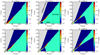 |
Fig. E.5 Same as Fig. E.4, but now dust grains have a high mm opacity. |
| In the text | |
|
Fig. E.6 Cut through the densities of the fiducial envelope-only and envelope-plus-disk model. The cut is in a direction just above where the disk is located to compare the densities in the envelope-only model and the envelope component of the envelope-plus-disk model. |
| In the text | |
|
Fig. E.7 Effect of viewing angle on the integrated line fluxes for the fiducial models. |
| In the text | |
|
Fig. E.8 Effect of viewing angle on the integrated line fluxes for the fiducial models with an envelope mass of 5 M⊙. |
| In the text | |
Current usage metrics show cumulative count of Article Views (full-text article views including HTML views, PDF and ePub downloads, according to the available data) and Abstracts Views on Vision4Press platform.
Data correspond to usage on the plateform after 2015. The current usage metrics is available 48-96 hours after online publication and is updated daily on week days.
Initial download of the metrics may take a while.