The Gravitational Wave Universe Toolbox

Shu-Xu Yi; Gijs Nelemans; Christiaan Brinkerink; Zuzanna Kostrzewa-Rutkowska; Sjoerd T. Timmer; Fiorenzo Stoppa; Elena M. Rossi; Simon F. Portegies Zwart

doi:10.1051/0004-6361/202141634

Home

All issues

Volume 663 (July 2022)

A&A, 663 (2022) A155

Full HTML

Free Access

Issue		A&A Volume 663, July 2022


Article Number		A155
Number of page(s)		22
Section		Numerical methods and codes
DOI		https://doi.org/10.1051/0004-6361/202141634
Published online		28 July 2022

A&A 663, A155 (2022)

A software package to simulate observations of the gravitational wave universe with different detectors^*,^**

Shu-Xu Yi (易疏序)¹^,5, Gijs Nelemans¹^,2^,3, Christiaan Brinkerink¹, Zuzanna Kostrzewa-Rutkowska¹^,2^,4, Sjoerd T. Timmer¹, Fiorenzo Stoppa¹, Elena M. Rossi⁴ and Simon F. Portegies Zwart⁴

¹ Department of Astrophysics/IMAPP, Radboud University, PO Box 9010, 6500 GL Nijmegen, The Netherlands
e-mail: sxyi@ihep.ac.cn
² SRON, Netherlands Institute for Space Research, Sorbonnelaan 2, 3584 CA Utrecht, The Netherlands
³ Institute of Astronomy, KU Leuven, Celestijnenlaan 200D, 3001 Leuven, Belgium
⁴ Leiden Observatory, Leiden University, PO Box 9513, 2300 RA Leiden, The Netherlands
⁵ Key Laboratory of Particle Astrophysics, Institute of High Energy Physics, Chinese Academy of Sciences, 19B Yuquan Road, Beijing 100049, PR China

Received: 25 June 2021
Accepted: 29 March 2022

Abstract

Context. As the importance of gravitational wave (GW) astrophysics increases rapidly, astronomers interested in GWs who are not experts in this field sometimes need to get a quick idea of what GW sources can be detected by certain detectors, and the accuracy of the measured parameters.

Aims. The GW-Toolbox is a set of easy-to-use, flexible tools to simulate observations of the GW universe with different detectors, including ground-based interferometers (advanced LIGO, advanced VIRGO, KAGRA, Einstein Telescope, Cosmic Explorer, and also customised interferometers), space-borne interferometers (LISA and a customised design), and pulsar timing arrays mimicking the current working arrays (EPTA, PPTA, NANOGrav, IPTA) and future ones. We include a broad range of sources, such as mergers of stellar-mass compact objects, namely black holes, neutron stars, and black hole–neutron star binaries, supermassive black hole binary mergers and inspirals, Galactic double white dwarfs in ultra-compact orbit, extreme-mass-ratio inspirals, and stochastic GW backgrounds.

Methods. We collected methods to simulate source populations and determine their detectability with various detectors. Our aim is to provide a comprehensive description of the methodology and functionality of the GW-Toolbox.

Results. The GW-Toolbox produces results that are consistent with previous findings in the literature, and the tools can be accessed via a website interface or as a Python package. In the future, this package will be upgraded with more functions.

Key words: gravitational waves / stars: neutron / stars: black holes / methods: numerical

^*

gw-universe.org

^**

https://bitbucket.org/radboudradiolab/gwtoolbox

© ESO 2022

1 Introduction

Gravitational wave (GW) astrophysics is quickly becoming a pivotal branch of astronomy. A growing number of researchers from different fields are becoming interested in GWs, finding them relevant to their various scientific goals (e.g. Petiteau et al. 2013; Lasky et al. 2016; Caprini & Figueroa 2018; Nelemans 2018; McWilliams et al. 2019; Barausse et al. 2020). The first frequency window to be made available covers ~ 10–1000 Hz (the ‘kHz band’), which corresponds to the working frequency range of ground-based interferometers, such as the operating second-generation detector known as the advanced Laser Interferometer Gravitational-Wave Observatory (LIGO)/Virgo interferometer (Virgo)/Kamioka Gravitational Wave Detector (KAGRA) (Harry & LIGO Scientific Collaboration 2010; Acernese et al. 2015; Kagra Collaboration 2019), and the planned third-generation detectors; for example, Einstein Telescope (ET, Punturo et al. 2010) and Cosmic Explorer (CE, Reitze et al. 2019). Space-borne interferometers, such as Laser Interferometer Space Antenna (LISA, Amaro-Seoane et al. 2017) and other similar projects, for example DECIGO (Kawamura et al. 2006), Taiji (Mei et al. 2020), and Tianqin (Luo et al. 2016), will cover the GW spectrum in the frequency range ~10⁻³–1 Hz (the ‘mHz band’). At even lower frequencies, pulsar timing arrays (PTAs, e.g., Hobbs & Dai 2017; Dahal 2020) are used to probe GWs with frequencies of around 10⁻⁸–10⁻⁵ Hz (the ‘nHz band’). There are also attempts to search for GWs at frequencies higher than the kHz regime, namely in MHz and GHz (Aggarwal et al. 2021). Although this frequency range is another important part of the GW Universe, which is full of opportunities to discover new physics and phenomena, we do not include detectors and sources of this frequency range in the GW-Toolbox at this stage because of the larger uncertainties involved.

Together, these detectors are sensitive to a very broad range of GW sources, where higher frequency detectors are sensitive to smaller objects. In the frequency range of ~ 10–1000 Hz, there are inspiral and mergers of stellar-mass compact-object binaries, spinning neutron stars, and supernova explosions (see e.g. Clark et al. 1979; Thorne 1987; Schutz 1989; Lipunov et al. 1997; Portegies Zwart & McMillan 2000; Belczynski et al. 2002; Ott 2009; Goetz & Riles 2011; Postnov & Yungelson 2014). On the other hand, the early inspiral phase of stellar-mass compact-object binaries occupies the frequency range of ~10⁻³–1 Hz (Sesana 2016). Also, white dwarf binaries, which are not compact enough to be detected by kHz detectors, are prominent sources for mHz detectors (e.g. Nelemans et al. 2001; Ruiter et al. 2010; Sesana 2016; Lamberts et al. 2018; Tauris 2018; Sesana et al. 2020; Lau et al. 2020). As BH size increases with mass, the mHZ detectors are sensitive to mergers of super-massive BHs (SMBHs: 10³–10⁸ M_⊙; e.g., Sesana et al. 2005; Berti et al. 2006) and extreme-mass-ratio inspirals (EMRIs; see Gair et al. 2004; Amaro-Seoane et al. 2007). Again, in the early inspiral phase, SMBH binaries occupy the low-frequency end of the spectrum of ~10⁻⁸–10⁻⁵ Hz, either as individual sources or as a stochastic background (Sazhin 1978; Detweiler 1979; Hellings & Downs 1983; Jenet et al. 2005; Sesana et al. 2008).

The first detection of GWs was made by the LIGO/Virgo Collaboration (LVC) in 2015 (Abbott et al. 2016a). The event GW150914 originates from the merger of a binary black hole (BBH) and was immediately recognised as having interesting astrophysical implications (see Abbott et al. 2016b; Belczynski et al. 2016). Since then, 90 GW events have been detected (as reported by LVC Abbott et al. 2019b, 2020c, Abbott et al. 2021b, and there are more candidates reported by other groups from the public strain data). These events include mergers of BBHs, double neutron stars (DNSs, e.g., GW170817 and GW190425), and black hole–neutron stars (BHNSs, e.g. GW190426, GW200105, and GW200115 Abbott et al. 2021a). The population of detected BBH mergers provides important information on stellar formation and evolution history (e.g. Abbott et al. 2021c). Among the detected sources, there are several unique systems that provide input to and even challenge current stellar evolution theory (e.g. GW190412, GW190814), and provide insight into the nature of neutron star matter (GW170817, GW190425). Multi-messenger observations of the DNS merger event GW170817/GRB 170817A/AT 2017gfo led to huge progress in astrophysics, fundamental physics, and cosmology (e.g. Abbott et al. 2017a,b,c,d,e,f, 2018b,a, 2019a,c,d, Abbott et al. 2020a; Coulter et al. 2017; Pian et al. 2017). Future detectors such as ET will vastly increase our detection reach and thus allow even broader scientific investigations (e.g. Maggiore et al. 2020).

Also, PTA observations are routinely happening, and although there has been no conclusive evidence of GW detection with PTA¹ so far, many authors are putting increasingly stringent upper limits on the nHz GW signals (van Haasteren et al. 2011; Demorest et al. 2013; Lentati et al. 2015; Arzoumanian et al. 2018; Verbiest et al. 2016; Aggarwal et al. 2019, Aggarwal et al. 2020) and have already ruled out some theories of galaxy evolution (Shannon et al. 2013, 2015). Future studies, in particular those including the Square Kilometre Array (SKA), will make significant progress in terms of experimental capability (e.g. Janssen et al. 2015).

In the following sections, we describe the GW-Toolbox, while in Sect. 5 we show results of its implementation and compare these to findings in the literature. In Sects. 6 and 7, we discuss the caveats involved with our software, outline our future plans, and summarise the findings of the present study.

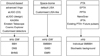Fig. 1

Summary of detectors and sources included in the GW–Toolbox.

2 The Gravitational Wave Universe Toolbox

The GW-Toolbox (website: gw-universe.org)² is a set of tools – for use by a broad audience – for quickly simulating observations of the GW universe with different detectors. Outputs include the expected number of detections, synthetic catalogues, and parameter uncertainties. We include three classes of GW detectors, namely Earth-based interferometers, spaceborne interferometers, and PTAs. In each of these classes, the GW-Toolbox has the following detectors with default and customised settings:

Earth-based interferometers:
- Advanced LIGO in O3.
- Advanced LIGO at final design sensitivity.
- Advanced Virgo at final design sensitivity.
- KAGRA.
- ET.
- CE.
- A LIGO/Virgo-Like interferometer with customised parameters.
Space-borne interferometers:
- Default LISA.
- LISA-like spacecraft with customised parameters.
PTAs:
- Existing EPTA.
- Existing PPTA.
- Existing NANOGrav.
- Existing IPTA.
- Any of the existing PTAs plus simulated new pulsars to mimic future PTAs.

The three classes of detectors correspond to the three main frequency regimes, namely kHz, mHz, and nHz. In the kHz GW regime, we include BBH mergers, DNS mergers, and BHNS mergers; in the mHz GW regime, we include supermassive binary black hole (SMBBH) mergers, close Galactic white dwarf (GWD) binary inspirals, and EMRIs (stellar mass BHs inspiraling into SMBHs); and in the nHz GW regime, we include individual SMBBH inspirals, and a stochastic GW background. See Fig. 1 for a summary of the detectors and sources. In practice, the logical flow of the GW-Toolbox is to first select the detector class and the detector parameters, and then choose the source class, select its parameters, and run. For some of the sources, the underlying cosmological model is also relevant to the simulation, where users are able to select a certain build-in cosmology or to input parameters for a self-defined Λ-CDM cosmological model. Examples in this paper are simulated with the cosmology model that corresponds to Planck DR15 (Planck Collaboration I 2016). We use the astropy package (Astropy Collaboration 2013, 2018) with the cosmology model ‘Planck15’. Changing to the more up-to-date ‘Planck18’ cosmology model does not significantly change the simulation catalogues.

The general outputs of the GW-Toolbox are the expected number of detections of the selected sources, and a synthetic catalogue with and without uncertainties on parameters. Plots and histograms of the parameters of the catalogue can be made in-browser, and the figures and catalogue can also be exported. Figure 2 shows a screen shot of the GW-Toolbox website with the top-level selection (left panel) and an example of the kHz detector selection page (right panel).

The aim of this paper is to provide a comprehensive description of the methodology and the functionality of the GW-Toolbox. The paper is organised with a similar structure as the setup of the GW-Toolbox. For each class of sources, a model of the Universe is made in which the sources are distributed in space, time, and other relevant parameters (such as mass, spin, etc.) according to a pre-defined population model. The user can change the population model according to a parametrised formalism. In Sect. 3, we give a description of each of the population models. The resulting GW source population is then observed in simulation by a selected GW detector from the above list. After both source and detector are determined, the sources detected during the simulation are selected using a signal-to-noise ratio (S/N) criterion. The uncertainties on the parameters of the detected sources are estimated using the Fisher Matrix formalism. In Sect. 4, we describe how the response of the detector is represented, and the algorithm used to generate the catalogue of detected sources. For PTAs, we describe our simplified representation of the pulsar array, the properties of the timing noises, and the observation campaign.

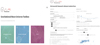Fig. 2

Screen shot of the GWT start page (left) and ground-based observatories page with results for advanced LIGO (right).

3 Implementation 1: The universe

We first turn to the implementation of the universe model, in which we select source population models from the literature and in some cases, allow users to change or adapt the source population. There are many reviews of GW sources that discuss these in more detail, such as Sathyaprakash & Schutz (2009) and González et al. (2013), and below we discuss the relevant ones. We start with sources for ground-based detectors, where we concentrate on compact binary mergers that are detectable with ground-based detectors, and then move to space-borne detectors, with SMBBH mergers, white dwarf compact binaries, and EMRIs as sources, and finish with PTAs for which we discuss individual SMBBHs as well as stochastic background.

3.1 Sources for ground-based detectors

There have been many studies of the formation and population of sources that are detectable with ground-based instruments (e.g. Phinney 1991; Schneider et al. 2001; Fryer & Kalogera 2001; Belczynski et al. 2002; Dominik et al. 2015; de Mink & Belczynski 2015) and population depends in a complicated way on many uncertain aspects of binary evolution, the formation of binary stars, and even the metallicity evolution of the cosmic star formation history. We take a simple, yet flexible approach, using a parametrised description of the source populations (but see e.g. Moe & Di Stefano 2017; Chruślińska et al. 2019, 2020 for discussions of some of the complications).

3.1.1 Binary black hole mergers

The population of BBH mergers is the most prominent of the sources observable by current GW detectors (Abbott et al. 2020c). The source population is characterised by the merger rate as a function of redshift and the distribution of masses and spins (e.g. Mapelli et al. 2017; Farr et al. 2011; Kovetz et al. 2017; Talbot & Thrane 2018; Postnov & Kuranov 2019; Abbott et al. 2019e).

In the population model for BBHs, the merger rate density is expressed as: $\dot{n} (z, m_{1}, q, χ) = ℛ (z) f (m_{1}) π (q) P (χ),$ ${h^{\ell m}} = {F_ + }h_ + ^{\ell m} + {F_ \times }h_ \times ^{\ell m}.$ (1)

where f (m₁) is the mass function of the primary (heavier) black hole, and π(q) and P(χ) are the probability distributions of the mass ratio q ≡ т₂/т₁ and the effective spin χ, respectively. $ℛ$ ${\cal R}$ as a function of z is often referred to as the cosmic merger rate density. We take the parameterisation as in Vitale et al. (2019): $ℛ (z_{m}) = ℛ_{n} \int_{z_{m}}^{\infty} ψ (z_{f}) P (z_{_{m}} | z_{f}) d z_{f},$ $\dot n\left( {z,{m_1},q,\chi } \right) = {\cal R}\left( z \right)f\left( {{m_1}} \right)\pi \left( q \right)P\left( \chi \right),$ (2)

where ψ(z) is the Madau-Dickinson star formation rate: $ψ (z) = \frac{{(1 + z)}^{α}}{1 + {(\frac{1 + z}{C})}^{β}},$ ${\cal R}\left( {{z_{\rm{m}}}} \right) = {{\cal R}_n}\int_{{z_{\rm{m}}}}^\infty {\psi \left( {{z_{\rm{f}}}} \right)} P\left( {{z_{_{\rm{m}}}}\left| {{z_{\rm{f}}}} \right.} \right){\rm{d}}{z_{\rm{f}}},$ (3)

with α = 2.7, β = 5.6, and С = 2.9 (Madau & Dickinson 2014), and P(z_m|z_f,τ) is the probability that the BBH merges at z_m if the binary is formed at z_f, which we refer to as the distribution of delay time with the form (Vitale et al. 2019): $P (z_{m} | z_{f}, τ) = \frac{1}{τ} \exp [- \frac{t_{f} (z_{f}) - t_{m} (z_{m})}{τ}] \frac{d t}{d z} .$ $\psi \left( z \right) = {{{{\left( {1 + z} \right)}^\alpha }} \over {1 + {{\left( {{{1 + z} \over C}} \right)}^\beta }}},$ (4)

In the above equation, t_f and t_m are the look-back times corresponding to z_f and z_m, respectively.

Figure 3 shows plots of $ℛ (z)$ ${\cal R}\left( z \right)$ with different $ℛ_{n}$ ${{\cal R}_n}$ and τ. The default parameters are set to $ℛ_{n}$ ${{\cal R}_n}$ = 13 Gpc⁻³ yr⁻¹ and τ = 3 Gyr, which are compatible with the local merger rate of BBHs found in ОЗа (Abbott et al. 2021c).

Although some information is known about the masses of the observed BBH (Abbott et al. 2021c), we assume a generic mass function p(m₁): $p (m_{1}) \propto {\begin{array}{l} \exp (\frac{c}{m_{1} - μ}) {(m_{1} - μ)}^{- γ}, & m_{1} \leq m_{cut} \\ 0, & m_{1} > m_{cut} \end{array} .$ $P\left( {{z_{\rm{m}}}|{z_{\rm{f}}},\tau } \right) = {1 \over \tau }\exp \left[ { - {{{t_{\rm{f}}}\left( {{z_{\rm{f}}}} \right) - {t_{\rm{m}}}\left( {{z_{\rm{m}}}} \right)} \over \tau }} \right]{{{\rm{d}}t} \over {dz}}.$ (5)

The distribution of p(m₁) is defined for m₁ > μ, which has a power law tail of index −γ and a cut-off above m_cut. When γ = 3/2, the distribution becomes a shifted Lévy distribution. p(m₁) peaks at m₁ = с/γ + μ. We set μ = 3, γ = 2.5, с = 6, m_cut = 95 M_⊙ as default, which results in a simulated catalogue that fits with the observed one (see Sect. 5.1). The normalisation of p(m₁) is: $Norm = c^{1 - γ} Γ (γ - 1, \frac{c}{m_{cut} - μ}),$ $p\left( {{m_1}} \right) \propto \left\{ {\matrix{ {\exp \left( {{c \over {{m_1} - \mu }}} \right){{\left( {{m_1} - \mu } \right)}^{ - \gamma }},} \hfill & {{m_1} \le {m_{{\rm{cut}}}}} \hfill \cr {0,} \hfill & {{m_1} > {m_{{\rm{cut}}}}} \hfill \cr } .} \right.$ (6)

where Γ(a, b) is the upper incomplete gamma function.

In order to provide more flexibility, we also provide an alternative p(m₁), which has an extra Gaussian peak component p_peak(m₁) in addition to the one in Eq. (5): $p_{peak} (m_{1}) = A_{peak} \exp [- {(\frac{m_{1} - m_{peak}}{σ_{peak}})}^{2}] .$ ${\rm{Norm}}\,{\rm{ = }}{c^{1 - \gamma }}\Gamma \left( {\gamma - 1,{c \over {{m_{{\rm{cut}}}} - \mu }}} \right),$ (7)

The normalisation of the alternative p(m₁) is: $Norm = c^{1 - γ} Γ (γ - 1, \frac{c}{m_{cut} - μ}) + {\sqrt{2 π σ}}_{peak} A_{peak} .$ ${p_{{\rm{peak}}}}\left( {{m_1}} \right) = {A_{{\rm{peak}}}}\exp \left[ { - {{\left( {{{{m_1} - {m_{{\rm{peak}}}}} \over {{\sigma _{{\rm{peak}}}}}}} \right)}^2}} \right].$ (8)

We denote the population models without and with the peak component in the mass function as BBH-PopA and BBH-PopB, respectively. Our default parameters for the peak component are A_peak = 0.002, m_реаk = 40 M_⊙, and σ_peak = 1 M_⊙, which are compatible with those implied from the third Gravitational-Wave Transient Catalogue (GWTC-3; Abbott et al. 2021b). Figure 4 shows mass distributions for BBH-PopA and BBH-PopB.

For π(q), we use a uniform distribution between [q_cut, 1] and assume χ follows a truncated Gaussian distribution centred at zero with standard deviation σ_χ, which is limited between −1 and 1 in accordance with general relativity. The actual mass ratio distribution is still poorly constrained from observations. The discovery of the GW190412 with asymmetric masses implies that the mass ratio distribution can be relatively broad (Abbott et al. 2020b). The Gaussian spin model is consistent with the findings of Abbott et al. (2021c). The default parameters we use are q_cut = 0.4 and σ_χ = 0.1. Those parameters in the population model can all be reset by users in both the web interface or in the Python package.

Fig. 3

$ℛ (z)$ ${\cal R}\left( z \right)$ , (Eq. (2)) with different $ℛ_{0}$ ${{\cal R}_0}$ and τ.

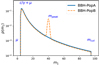Fig. 4

Primary BH mass distribution in the default models of BBH-PopA/B; see Eqs. (5) and (7). Here we mark μ, μ + с/γ, and m_реа in the plot in order to provide a rough estimate of these quantities.

3.1.2 DNS mergers

For the population model of DNS mergers, the merger rate density is similarly expressed as: $\dot{n} (z, m_{a}, m_{b}, χ) = ℛ (z) p (m_{a}) p (m_{b}) p (χ),$ ${\rm{Norm}}\,{\rm{ = }}{c^{1 - \gamma }}{\rm{\Gamma }}\left( {\gamma - 1,{c \over {{m_{{\rm{cut}}}} - \mu }}} \right) + {\sqrt {2\pi \sigma } _{{\rm{peak}}}}{A_{{\rm{peak}}}}.$ (9)

where $ℛ (z)$ ${\cal R}\left( z \right)$ takes the same form as in the BBH population model, but with a different default setting: $ℛ_{n} = 300 {Gpc}^{- 3} {yr}^{- 1}$ ${{\cal R}_n} = 300\,{\rm{Gp}}{{\rm{c}}^{ - 3}}\,{\rm{y}}{{\rm{r}}^{ - 1}}$ and τ = 3 Gyr, which are compatible with the local merger rate of DNS s found with GWTC-2; р(т_a,b) is the mass function of the neutron stars. We note that we use т_a,b instead of m_1,2 The latter represents the primary and secondary stars based on their masses, whilst the former does not distinguish between primary and secondary stars. We assume both m_a and m_b are following the same mass function. We use a truncated Gaussian with upper and lower cuts as the mass function. The default parameters are the mean $\bar{m} = 1.4 M_{⊙}$ $\bar m = 1.4{M_ \odot }$ , the mass dispersion σ_m = 0.5 M_⊙, and the lower and upper mass limits m_cut,low = 1.1 M_⊙, m_cut,high = 2.5 M_⊙; we also apply a truncated Gaussian spin model with a smaller dispersion σ_χ = 0.05. These simplified choices roughly agree with observations (Valentim et al. 2011; Özel et al. 2012; Kiziltan et al. 2013; Miller & Miller 2015; Farrow et al. 2019; Zhang et al. 2019), while they can be substituted with more realistic models.

3.1.3 BHNS mergers

For the population model of BHNS mergers, we again assume the merger rate density to be: $\dot{n} (z, m_{1}, m_{2}, χ) = ℛ (z) f (m_{•}) p (m_{n}) p (χ),$ $\dot n\left( {z,{m_a},{m_b},\chi } \right) = {\cal R}\left( z \right)p\left( {{m_a}} \right)p\left( {{m_b}} \right)p\left( \chi \right),$ (10)

where $ℛ (z)$ ${\cal R}\left( z \right)$ takes the same form as for BBHs and DNSs, with a different default setting: $ℛ_{n} = 45 {Gpc}^{- 3} {yr}^{- 1} and τ = 3 Gyr$ ${{\cal R}_n} = 45\,{\rm{Gp}}{{\rm{c}}^{ - 3}}\,{\rm{y}}{{\rm{r}}^{ - 1}}\,{\rm{and}}\,\tau = {\rm{3}}\,{\rm{Gyr}}$ ; which is broadly consistent with the merger rate, which itself is implied by the number of BHNS s detected in LIGO-Virgo-KAGRA (LVK) 03a+b (Abbott et al. 2021a). Also, f(m_●) is the mass function of the BH, which takes the same function form as in Eqs. (5) and (7). We denote the population model without and with the peak component in f(m_●) as BHNS-PopA and BHNS-PopB, respectively; The default parameters for f(m_●) are μ = 3, γ = 2.5, с = 6, m_cut = 95 M_⊙, A_peak = 0.002, m_реа= 40 M_⊙, and σ_peak = 1M_⊙. Here, p(m_n) is the mass function of the NS, which is the same as in the DNS case.

3.2 Sources for space-borne detectors

3.2.1 Supermassive black hole binaries

In the last two decades, it has been established that in the centre of most galaxies there is a SMBH with a mass of between 10⁴ M_⊙ and 10¹⁰ M_⊙. As galaxy mergers are thought to be ubiquitous under the hierarchical clustering process, there are expected to be close binaries of SMBHs, that is, SMBBHs, in the merger galaxies, which emit GWs during their inspirai and merger phase (e.g. Colpi 2014). Such SMBBH inspirais are the main targets of LISA (Amaro-Seoane et al. 2017), TianQin (Luo et al. 2016), and PTA (Jenet et al. 2004, Jenet et al. 2005), as the frequency of their GWs falls in the 10⁻⁸–1 Hz range. We use the SMBBH merger catalogues from Klein et al. (2016) (Klein 16 hereafter), which are based on Barausse (2012). There are three population models being considered in Klein l6, namely рорЗ, Q3_nodelays, and Q3_delays, which mainly differ in the origin of their SMBH seeds, and whether or not the delays between SMBH mergers and galaxy mergers are included (see Kleinló for a detailed description; see also a review on SMBH formation and evolution by Inayoshi et al. 2020). For рорЗ, the SMBH seeds are from PopIII stars (light seeds), and the delay between SMBH and galaxy mergers is accounted for; for Q3_nodelays and Q3_delays, the SMBH seeds are assumed to be from the collapse of pro-togalactic disks (heavy seeds). The former accounts for the delay between SMBH and galaxy mergers, while the latter does not. For each population model, there are ten catalogues, each corresponding to a realisation of all sources in the Universe within 5 yr. The number of total events for each population is ~890 for рорЗ, ~630 for Q3_nodelays, and ~40 for Q3_delays. These values are compatible with the reported average merger rates in Klein l6 (рорЗ: 175.36 yr⁻¹, Q3_nodelays: 121.8yr⁻¹ and Q3_delays: 8.18 yr⁻¹). Figure 5 shows M_z,tot (redshifted total mass) as a function of z for SMBBH mergers that occur in the universe over a timescale of 5 yr for three population models as a direct demonstration of the population models. The distributions agree with those shown in Fig. 3 of Klein 16.

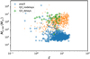Fig. 5

M_Z,tot vs. z of SMBBH mergers that occur in the Universe over a timescale of 5 yr for three population models from Klein 16. The data correspond to one realisation.

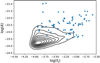Fig. 6

Distribution density of GW properties of DWD binaries in the simulated catalogue (black contours) as function of GW frequency f_s and GW amplitude A. The blue stars are known DWDs used as VBs.

3.2.2 Double white dwarfs

Another important population of LISA sources are ultra-compact Galactic binaries. Among those Galactic binaries, close double white dwarfs (DWDs) are the dominant population and have long been expected to be promising targets for LISA and other space-borne GW detectors (e.g. Nelemans et al. 2001; Yu & Jeffery 2010; Nissanke et al. 2012; Toonen et al. 2012; Korol et al. 2017; Lamberts et al. 2019; Huang et al. 2020).

We use a synthetic catalogue of close DWDs in the whole Galaxy (Nelemans et al. 2001). Figure 6 shows the joint distribution density of the frequencies f_s = 2/P (where P is the orbital period of the binaries) and the intrinsic amplitudes $A = 2 {(G ℳ)}^{5 / 3} {(π f)}^{2 / 3} / (c^{4} d)$ $A = 2{\left( {G{\cal M}} \right)^{{5 \mathord{\left/ {\vphantom {5 3}} \right. \kern-\nulldelimiterspace} 3}}}{{{{\left( {\pi f} \right)}^{{2 \mathord{\left/ {\vphantom {2 3}} \right. \kern-\nulldelimiterspace} 3}}}} \mathord{\left/ {\vphantom {{{{\left( {\pi f} \right)}^{{2 \mathord{\left/ {\vphantom {2 3}} \right. \kern-\nulldelimiterspace} 3}}}} {\left( {{c^4}d} \right)}}} \right. \kern-\nulldelimiterspace} {\left( {{c^4}d} \right)}}$ of GWs emitted from binaries in the catalogue. The contours mark levels corresponding to uniform iso-proportions of the density. The total number of sources in the catalogue is ~2.6× 10⁷.

Besides the synthetic catalogue, we also include a catalogue of 81 known DWDs (Huang et al. 2020) known as verification binaries (VBs; see also Kupfer et al. 2018). Those VBs are plotted in Fig. 6 with star markers. We note that the distribution of the VBs does not follow that of the simulated DWDs in the whole Galaxy because of very strong observational biases that favour the detection of close-by sources and therefore there use as VBs.

Fig. 7

The averaged histograms of μ, M and D of EMRIs happen in 1 yr, assuming different population models from Babak l7.

3.2.3 Extreme mass-ratio inspirais

In general, in the nucleus of a galaxy, surrounding the SMBH, there is an abundant stellar population. In certain instances, compact objects, including stellar-mass BHs, NSs, and WDs, can inspirai into the central SMBH, radiating a large amount of energy in GWs. These systems are referred to as EMRIs, and are very interesting targets for space-borne detectors such as LISA (see Amaro-Seoane et al. 2007). In the GW-Toolbox, we use the simulated catalogues from Babak et al. (2017) (Babak 17 hereafter) and use their population models M1-M11 (skipping M7, the reason for which we explain below). These populations differ in terms of several parameters and/or their relationships: the mass function and spin distribution of SMBHs, the M–σ relation, the ratio of plunges to EMRIs, and the characteristic mass of the compact objects (see Babak 17 for a detailed description of models). For each population model, there are ten realisations of the catalogues, which contain detectable EMRIs within 1 yr with the assumption of standard LISA noise properties. The distributions of μ (mass of the stellar BH), M (mass of the massive BH), and D (luminosity distance) in the catalogues are plotted in Fig. 7. The histogram for each population is an average over the ten realisations. As we are using an S/N-limited sample, instead of a complete sample of the whole Universe (which is about ten times larger), the GW-Toolbox will give an underestimated detectable number and an incomplete catalogue of detections, especially when using a lower S/N cutoff or a more sensitive LISA configuration. For now, we exclude M7 and M12 from the Toolbox, because in their population models the direct plunges are ignored, and therefore the total number of EMRIs is about one order of magnitude larger than those in other population models, which makes the computation prohibitively time-consuming.

3.3 Sources for PTAs

3.3.1 Individual massive black hole

Gravitational waves from SMBBHs lie in the PTA frequency range long before (millions or tens of millions of years, depending on their chirp mass; see Sesana & Vecchio 2010; Petiteau et al. 2013; Burke-Spolaor et al. 2019) they enter the band of space-borne GW detectors. If there were such MBH binaries sufficiently close to Earth, PTAs could detect their signals. As no such sources are known yet, we incorporate this source class into the GW-Toolbox in the form of a free form in which the user can fill in the frequency and GW amplitude, and the GW-Toolbox will determine if this binary, as a monochromatic GW source, can be detected by the selected PTA.

3.3.2 Stochastic background

The second class of targets for PTA are known as stochastic GW background (SGWB). Such ‘objects’ can originate from the incoherent overlapping of many unresolvable SMBBHs (Phinney 2001; Sesana et al. 2008; McWilliams et al. 2014), the relic of primordial GWs (Grishchuk 1976, 1977; Linde 1982; Starobinsky 1980), or the collision of cosmic strings (Damour & Vilenkin 2001, 2005; Siemens et al. 2006, 2007; Ölmez et al. 2010). Each of these gives rise to a power-law GW signal $h_{c}^{2} (f) = C f^{γ},$ $\dot n\left( {z,{m_1},{m_2},\chi } \right) = {\cal R}\left( z \right)f\left( {{m_ \bullet }} \right)p\left( {{m_n}} \right)p\left( \chi \right),$ (11)

where the index γ corresponds to the origin of the SGWB. For incoherent overlapping of SMBBHs, γ = −2/3; for relic GWs, γ = −1; and for cosmic strings, γ = −7/6. We also enable users to customise γ.

4 Implementation 2: Gravitational wave detectors

4.1 Ground-based interferometers

4.1.1 Noise model of interferometers

For ground-based interferometers, the GW-Toolbox integrates the design performance of advanced LIGO (aLIGO), Advanced Virgo (AdV), KAGRA, CE, and ET instruments. The noise models for the above-mentioned interferometers are taken from the following resources: aLIGO: https://dcc.ligo.org/LIGO-T1800044/public, see also The LIGO Scientific Collaboration (2015); adV and KAGRA: https://dcc.ligo.org/LIGO-T1500293/public; CE: https://dcc.ligo.org/LIGO-P1600143/public; ET: http://www.et-gw.eu/index.php/etsensitivities, see also Hild et al. (2008, 2010, 2011).

The upper panel of Fig. 8 shows the noise curves used for the default detectors. aLIGO-03 corresponds to the noise performance in the O3 period, while aLIGO-design is the designed sensitivity of the aLIGO; CE1 and CE2 correspond to the expected first and second stages of CE, respectively; ET we use the ET-D-sum curve.

In addition, the GW-Toolbox employs the package FINESSE to calculate S_n of a LIGO-like or an ET-like interferometer with customised settings (Brown et al. 2020). Users can define the following parameters of the detector: arm length, laser power, arm mirror mass, arm mirror transmission coefficient, signal recycling mirror transmission coefficient, power recycling mirror transmission coefficient, signal recycling phase factor, power recycling cavity length, signal recycling cavity length. The most important parameters that affect the sensitivity are arm length and laser power. The lower panel of Fig. 8 shows the effects of varying arm length and laser power starting from the designed aLIGO sensitivity. One of the other influential parameters is the mass of the arm mirror. Heavier arm mirrors decrease the noise in the low-frequency end of the slope and leave the high-frequency end unaffected.

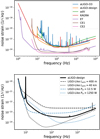Fig. 8

Upper panel: noise curves of the default detectors. Lower panel: aLIGO in design vs. customised settings (arm length = 4km, laser power = 125 W).

4.1.2 Signal-to-noise ratio of GWs from compact binary mergers

The core of the method with which the GW-Toolbox determines the detectability of a source is a comparison between the S/N threshold ρ_⋆ and the S/N of the source, which can be calculated with (Maggiore 2008): $ρ^{2} = 4 \int_{f_{low}}^{f_{high}} \frac{| h^{2} (f) |}{S_{n} (f)} d f,$ $h_{\rm{c}}^2\left( f \right) = C{f^\gamma },$ (12)

where h(f) is the frequency domain response of the interferometer to the GW signal, and S_n is the noises power density. For a binary system, the detector response can be expressed as³: $h (f) = c \sqrt{{(\frac{1 + \cos^{2} l}{2})}^{2}} F_{+}^{2} + \cos l^{2} F_{\times}^{2} A (f) e^{- i (Ψ (f) + ϕ_{p})} .$ ${\rho ^2} = 4\,\int_{{f_{{\rm{low}}}}}^{{f_{{\rm{high}}}}} {{{\left| {{h^2}\left( f \right)} \right|} \over {{S_{\rm{n}}}\left( f \right)}}{\rm{d}}f,}$ (13)

In the above equation, the constant $c = \frac{1}{2} \sqrt{\frac{5}{6}} \frac{{(G ℳ)}^{5 / 6}}{c^{3 / 2} π^{2 / 3} D_{L}},$ $h\left( f \right) = c\sqrt {{{\left( {{{1 + {{\cos }^2}\,l} \over 2}} \right)}^2}} F_ + ^2 + \cos \,{l^2}F_ \times ^2A\left( f \right){{\rm{e}}^{ - i\left( {{\rm{\Psi }}\left( f \right) + {\phi _{\rm{p}}}} \right)}}.$ (14)

where $ℳ$ ${\cal M}$ is the redshifted chirp mass of the binary, D_L is the luminosity distance, i is the inclination angle between the orbital angular momentum and the line of sight, and A(f) is the frequency dependence of the GW amplitude. As a proof of principle of the GW-Toolbox, we apply the waveform approximant, which has hybrid degrees of simplification. For the amplitude A(f), we use a broken power law: $A (f) = {\begin{array}{l} f^{- 7 / 6}, & f \leq f_{trans}, \\ f^{- 2 / 3}, & w_{m} f_{trans} & < f \leq f_{cut}, \\ 0, & f \geq f_{cut}, \end{array}$ $c = {1 \over 2}\sqrt {{5 \over 6}} {{{{\left( {G{\cal M}} \right)}^{5/6}}} \over {{c^{3/2}}{\pi ^{2/3}}{D_{\rm{L}}}}},$ (15)

where w_m is the scaling factor needed to make A(f) continuous. The above formula represents the inspirai, merger, and ring-down phases of a circular, non-spinning point mass binary. It corresponds to the A(f) in the approximant IMRPhenomD (Ajith et al. 2011), when the effective spin χ = 0. The transition frequency_trans and the cut-off frequency f_cut correspond to f₁ and f₂ of Ajith et al. (2011). A(f) and т₁, т₂, and D via С essentially determine the S/N of a source, because the effective spin has a much weaker effect on the S/N. Therefore, the dependence on χ can be separated from that on т₁, т₂, or D. This makes the catalogue-sampling process easier and more effective (the Markov chain takes less time to mix with fewer dimensions, see below).

Ψ(f) is the phase of the waveform, and is essential for evaluating the uncertainties on the intrinsic parameters. Therefore, we use Ψ(f) from the frequency domain waveform IMRPhenomD (Ajith et al. 2011) and restore its dependency on χ- It corresponds to a hybrid waveform of a circular binary with parallel spin, which matches post-Newtonian and numerical relativity waveforms.

F_+,× are the antenna patterns of the interferometer, which are a function of the position angles of the source (θ,φ) and the polarization angle of the GW ψ, For LIGO-, Virgo-, and KAGRA-like interferometers, each of which have two perpendicular arms, the antenna patterns are: $\begin{array}{l} F_{+, 90 °} & = & \frac{1}{2} (1 + \cos^{2} θ) \cos 2 φ \cos 2 ψ + \cos θ \sin 2 φ \sin 2 ψ \\ F_{\times, 90 °} & = & \frac{1}{2} (1 + \cos^{2} θ) \cos 2 φ \sin 2 ψ + \cos θ \sin 2 φ \cos 2 ψ \end{array}$ $A\left( f \right) = \left\{ {\matrix{ {{f^{ - 7/6}},} \hfill & {f \le {f_{{\rm{trans}}}},} \hfill & {} \hfill \cr {{f^{ - 2/3}},} \hfill & {{w_{\rm{m}}}{f_{{\rm{trans}}}}} \hfill & { lt; f \le {f_{{\rm{cut}}}},} \hfill \cr {0,} \hfill & {f \ge {f_{{\rm{cut}}}},} \hfill & {} \hfill \cr } } \right.$ (16)

and for ET-like interferometers with 60° angles between the arms (Regimbau et al. 2012), $\begin{array}{l} F_{+, 60 °} & = & - \frac{\sqrt{3}}{2} F_{+, 90 °} \\ F_{\times, 60 °} & = & \frac{\sqrt{3}}{2} F_{\times, 90 °} . \end{array}$ $\matrix{ {{F_{ + ,90^\circ }}} \hfill & = \hfill & {{1 \over 2}\left( {1 + {{\cos }^2}\theta } \right)\cos 2\varphi \cos 2\psi + \cos \theta \sin 2\varphi \sin 2\psi } \hfill \cr {{F_{ \times ,90^\circ }}} \hfill & = \hfill & {{1 \over 2}\left( {1 + {{\cos }^2}\theta } \right)\cos 2\varphi \sin 2\psi + \cos \theta \sin 2\varphi \cos 2\psi } \hfill \cr }$ (17)

An ET will have three nested interferometers, each rotated by 60^° with respect to the others. The antenna pattern for each interferometer is F_{i,+, ×} (θ, φ, ψ) = F_{0,+, ×} (θ, φ + 2/3iπ, ψ), where i = 0, 1, 2 are the indexes of the interferometers, and F_{0,+, ×} are those in Eq. (17). The joint response can be calculated with Eq. (13), where the antenna pattern squared should be substituted with: $F_{+, \times}^{2} = \sum_{i = 0}^{2} F_{i, +, \times}^{2} .$ $\matrix{ {{F_{ + ,60^\circ }}} \hfill & = \hfill & { - {{\sqrt 3 } \over 2}{F_{ + ,90^\circ }}} \hfill \cr {{F_{ \times ,60^\circ }}} \hfill & = \hfill & {{{\sqrt 3 } \over 2}{F_{ \times ,90^\circ }}.} \hfill \cr }$ (18)

In our treatment, the modulation of the antenna pattern due to the rotation of Earth is neglected, because the duration of the GW signal is typically much shorter than the period of Earth’s rotation. The situation would change for 3G detectors, which have a much broader frequency window and the ability to better resolve the waveform.

4.1.3 Determining the sample of detected sources

Given the differential cosmic merger rate density for compact binary mergers, $\dot{n}$ ${\dot n}$ , the theoretical number distribution for each source class in the catalogue is: $N_{D} (Θ, θ, φ, ψ, l) = \frac{Δ T}{1 + z} \frac{d V_{c}}{4 π dz} \dot{n} (Θ, θ, φ, l, ψ) ℋ (ρ^{2} - ρ_{⋆}^{2}),$ $F_{ + , \times }^2 = \sum\limits_{i = 0}^2 {F_{i, + , \times }^2.}$ (19)

where ∆T is the time-span of observation, dV_c/dz is the differential cosmic comoving volume (volume per redshift), $ℋ$ ${\cal H}$ is the Heaviside step function, and ρ_⋆ is the S/N threshold, and Θ denotes the intrinsic parameters and the luminosity distance of the source. Marginalising over the directional parameters and assuming that n is isotropic yields $N_{D} (Θ) = \frac{T}{1 + z} \frac{d V_{c}}{dz} \dot{n} (Θ) D (Θ),$ ${N_D}\left( {{\rm{\Theta }},\theta ,\varphi ,\psi ,l} \right) = {{{\rm{\Delta }}T} \over {1 + z}}{{{\rm{d}}{V_{\rm{c}}}} \over {4\pi {\rm{dz}}}}\dot n\left( {{\rm{\Theta }},\theta ,\varphi ,l,\psi } \right){\cal H}\left( {{\rho ^2} - \rho _ \star ^2} \right),$ (20)

where $D (Θ) = ∯ dΩd Ω^{'} ℋ (ρ^{2} - ρ_{⋆}^{2}) / {(4 π)}^{2}$ ${N_D}\left( {\rm{\Theta }} \right) = {T \over {1 + z}}{{{\rm{d}}{V_{\rm{c}}}} \over {{\rm{dz}}}}\dot n\left( {\rm{\Theta }} \right){\cal D}\left( {\rm{\Theta }} \right),$ (21)

is the detectability of the source, which is determined by the detector properties and the waveform of the source. As we use the same waveform for BBHs, DNSs, and BH-NSs, the difference between these three populations is only in the cosmic merger rate $\dot{n}$ ${\dot n}$ discussed above in Sects. 3.1.1–3.1.3.

The total number of expected events in the catalogue is $N_{tot} = \int dΘ N_{D} (Θ),$ ${\cal D}\left( {\rm{\Theta }} \right) = \mathop{{\int\!\!\!\!\!\int}\mkern-21mu \bigcirc} {{\rm{d\Omega d\Omega '}}} {\cal H}\left( {{\rho ^{\rm{2}}} - \rho _ \star ^{\rm{2}}} \right)/{\left( {4\pi } \right)^2}$ (22)

and the number of detections is therefore a Poisson realisation of the expectation value N_D(Θ). The synthetic catalogue is then obtained by a Markov chain-Monte Carlo sampling from N_D(Θ). We apply the elliptical slice sampling algorithm (Murray et al. 2010), which takes less time to converge to the target distribution than the traditional Metropolis-Hasting algorithm (Neal et al. 1999) and requires less tuning of the initial parameters.

We also give the estimated uncertainties on the parameters using the Fisher information matrix (FIM): the covariance matrix is related to the Fisher matrix with: $〈 δ Θ_{i} δ Θ_{j} 〉 = ℱ_{i j}^{- 1},$ ${N_{{\rm{tot}}}} = \int {{\rm{d\Theta }}{N_{\rm{D}}}\left( {\rm{\Theta }} \right),}$ (23)

where the Fisher matrix is defined as: $ℱ_{i j} = (\partial h / \partial Θ_{i} | \partial h / \partial Θ_{j}) .$ $\left\langle {\delta {{\rm{\Theta }}_i}\delta {{\rm{\Theta }}_j}} \right\rangle = {\cal F}_{ij}^{ - 1},$ (24)

The partial derivatives in the above equation are calculated numerically: $\frac{\partial h}{\partial Θ_{i}} = \frac{h (Θ_{i} + {ΔΘ}_{i}) - h (Θ_{i} - {ΔΘ}_{i})}{2 {ΔΘ}_{i}} .$ ${{\cal F}_{i\,j}} = \left( {\partial h/\partial {{\rm{\Theta }}_i}\left| {\partial h/\partial {{\rm{\Theta }}_j}} \right.} \right).$ (25)

In the GW-Toolbox, we use ∆Θ_i = 10⁻⁸Θ_i, as it is sufficiently small to give stable results. We only calculate the FIM for intrinsic parameters (m_1,z, m_2,z and χ) and an overall scaling factor that represents the effect of all extrinsic parameters. As a result, we cannot give an estimate of the uncertainties on extrinsic parameters, such as the distance, sky locations, inclination, and polarisation angle, because these parameters contribute to the overall scaling factor in a highly correlated way. In reality, the sky locations are determined largely by triangulation with a network of detectors, and the precision of other extrinsic parameters also depend on triangulation. In the current version of the GW-Toolbox, we do not include a detector network. The calculation of the FIM is therefore simplified. However, in order to obtain an estimation of the uncertainties on the source frame masses, one still needs to propagate the uncertainty on the redshift. The uncertainty on the redshift itself is also an interesting quantity that users will want to obtain from the synthetic catalogue of GW-Toolbox. We provide an evaluation of ôz from empirical relations. For 2G detectors, we use δz = 0.5z, which roughly represents the trend of δz − z in GWTC-3; for 3G detectors, we use δz = 0.017z + 0.012, which is a fit from the simulation results of Vitale & Evans (2017). Also, δz is propagated to the uncertainties on the source frame masses with the following equation: $δ m_{i} = m_{i} \sqrt{{(\frac{δ m_{i, z}}{m_{i, z}})}^{2} + {(\frac{δ z}{1 + z})}^{2}} .$ ${{\partial h} \over {\partial {{\rm{\Theta }}_i}}} = {{h\left( {{{\rm{\Theta }}_i} + {\rm{\Delta }}{{\rm{\Theta }}_i}} \right) - h\left( {{{\rm{\Theta }}_i} - {\rm{\Delta }}{{\rm{\Theta }}_i}} \right)} \over {2{\rm{\Delta }}{{\rm{\Theta }}_i}}}.$ (26)

It is worth mentioning that although FIM is a quick, simple, and widely applied method for calculating uncertainties, it sometimes provides overestimated uncertainties compared to those from full Bayesian inference (e.g. Veitch et al. 2015), especially for events with low S/N (e.g. Vallisneri 2008; Rodriguez et al. 2013).

The returned catalogue is composed of mean values of the parameters and their estimated uncertainties. A more realistic simulation of the observed catalogue can be obtained by shifting the mean values according to the corresponding uncertainties, which is straightforward and easy. As the uncertainties given here are conservative, the GW-Toolbox returns the unshifted catalogue, and lets the user to decide whether or not and how to further shift the catalogue.

4.2 Space-borne interferometers

The space-borne interferometers module of the Toolbox enables users to simulate observations with LISA-like space-borne GW observatories (see Barke et al. 2015). We work with the codes of the LISA Data Challenge (LDC, https://lisa-ldc.lal. in2p3.fr, a successor program of the earlier Mock LISA Data Challenge; Babak et al. 2010), and make it possible for users to customise the arm length, the laser power, and the telescope diameter of LISA. In the ground-based interferometers section, the theoretical probability distributions of parameters of the detectable sources are first calculated. Samples are then drawn from these distributions as synthetic catalogues of observations. The procedure for LISA-like detectors is different: we go through pre-generated synthetic catalogues of different source populations in the whole Universe or Galaxy and then calculate the S/N of each source to be detected by LISA. The S/N is still calculated with: $ρ^{2} = 4 \int \frac{| h^{2} (f) |}{S_{n} (f)} d f,$ $\delta {m_i} = {m_i}\sqrt {{{\left( {{{\delta {m_{i,z}}} \over {{m_{i,z}}}}} \right)}^2} + {{\left( {{{\delta z} \over {1 + z}}} \right)}^2}} .$ (27)

where h(f) is the LISA response to a waveform of a source, and S_n(f) is the noise power spectrum density (PSD). The time-delay interference (TDI) channels are combinations of data streams such that the noise arising from the fluctuation of the laser frequency can be exactly cancelled while the GW signal can be preserved (Tinto & Armstrong 1999; Armstrong et al. 1999; Estabrook et al. 2000). In the GW-Toolbox, we consider the LISA responses and the noise spectral density in the first generation TDI-X channel (Armstrong et al. 1999). The noise spectrum is introduced in the following section. Three classes of sources are included in the GW-Toolbox for LISA, namely mergers of SMBBHs, resolved DWDs in the Galaxy, and EMRIs. Waveforms and the corresponding LISA responses are introduced in the following subsections. Examples of synthetic observations are given and compared with the literature in Sect. 5. Uncertainties on the parameters are again estimated with the FIM method.

4.2.1 Noise TDI

The PSD of the noise TDI-X response is formulated as in Armstrong et al. (1999) as $S_{X} (f) = [4 \sin^{2} (2 x) + 32 \sin^{2} x] S_{y}^{accel} + 16 \sin^{2} x S_{y}^{optical},$ ${\rho ^2} = 4\int {{{\left| {{h^2}\left( f \right)} \right|} \over {{S_{\rm{n}}}\left( f \right)}}{\rm{d}}f,}$ (28)

where x = 2πfL/c, L is the arm length of LISA, c is the speed of light, and $S_{y}^{accel}$ $S_y^{{\rm{accel}}}$ and $S_{y}^{optical}$ $S_y^{{\rm{optical}}}$ are the fractional frequency fluctuations due to the acceleration noise of the spacecraft and the optical meteorology system noise, respectively. For the acceleration noise, we use (Amaro-Seoane et al. 2017) $S_{a}^{accel} = 9 \times 10^{- 30} \frac{{[m s^{- 2}]}^{2}}{[Hz]} (1 + {(\frac{[0.4 mHz]}{f})}^{2}) (1 + {(\frac{f}{[8 mHz]})}^{4}) .$ ${S_X}\left( f \right) = \left[ {4{{\sin }^2}\left( {2x} \right) + 32{{\sin }^2}x} \right]S_y^{{\rm{accel}}} + 16{\sin ^2}xS_y^{{\rm{optical}}},$ (29)

We note that the above noise is in the form of acceleration; to convert this into a fractional frequency fluctuation, it must be divided by a factor 4π²f²c² (Armstrong et al. 1999), resulting in $S_{y}^{accel}$ $S_a^{{\rm{accel}}} = 9 \times {10^{ - 30}}{{{{\left[ {m{{\rm{s}}^{ - 2}}} \right]}^2}} \over {\left[ {{\rm{Hz}}} \right]}}\left( {1 + {{\left( {{{\left[ {0.4{\rm{mHz}}} \right]} \over f}} \right)}^2}} \right)\left( {1 + {{\left( {{f \over {\left[ {8{\rm{mHz}}} \right]}}} \right)}^4}} \right).$ (30) $= \frac{3.9 \times 10^{- 44}}{[Hz]} (1 + {(\frac{[0.4 mHz]}{f})}^{2}) ({(\frac{[8 mHz]}{f})}^{2}) + (1 + {(\frac{f}{[8 mHz]})}^{2}) .$ $S_y^{{\rm{accel}}}$ (31)

The noise of the optical metrology system can be split as follows: $S_{y}^{optical} = S^{ops} + S^{opo},$ $= {{3.9 \times {{10}^{ - 44}}} \over {\left[ {{\rm{Hz}}} \right]}}\left( {1 + {{\left( {{{\left[ {0.4{\rm{mHz}}} \right]} \over f}} \right)}^2}} \right)\left( {{{\left( {{{\left[ {8{\rm{mHz}}} \right]} \over f}} \right)}^2}} \right) + \left( {1 + {{\left( {{f \over {\left[ {8{\rm{mHz}}} \right]}}} \right)}^2}} \right).$ (32)

where S^ops is the laser shot noise, which scales with the arm length L, the laser power P, and the diameter of the telescope D as (Amaro-Seoane et al. 2017): $S^{ops} = 5.3 \times 10^{- 38} \times {(\frac{f}{[Hz]})}^{2} \frac{[2 W]}{P} {(\frac{L}{2.5 [Gm]})}^{2} {(\frac{[0.3 m]}{D})}^{2} {Hz}^{- 1}$ $S_y^{{\rm{optical}}} = {S^{{\rm{ops}}}} + {S^{{\rm{opo}}}},$ (33)

and $S^{opo} = 2.81 \times 10^{- 38} {(f / [Hz])}^{2} {Hz}^{- 1}$ ${S^{{\rm{ops}}}} = 5.3 \times {10^{ - 38}} \times {\left( {{f \over {\left[ {{\rm{Hz}}} \right]}}} \right)^2}{{\left[ {2W} \right]} \over P}{\left( {{L \over {2.5\left[ {{\rm{Gm}}} \right]}}} \right)^2}{\left( {{{\left[ {0.3{\rm{m}}} \right]} \over D}} \right)^2}{\rm{H}}{{\rm{z}}^{ - 1}}$ (34)

denotes the contribution from other noise in the optical meteorology system.

We also include the TDI-X noise PSD originating from the foreground GW emission from Galactic DWDs (GWD). In practice, this confusion noise will be modulated with the orbital phase of the spacecraft. For simplicity, we adopt an analytic approximation for the average equal-arm Michelson PSD of GWD as in Robson et al. (2019) as: $S_{GWD} (f, T_{obs}) = A f^{- 7 / 3} e^{- f^{α} + β f \sin (k f)} (1 + \tanh (γ (f_{k} - f)))$ ${S^{{\rm{opo}}}} = 2.81 \times {10^{ - 38}}{\left( {f/\left[ {{\rm{Hz}}} \right]} \right)^2}{\rm{H}}{{\rm{z}}^{ - 1}}$ (35)

We note that the noise depends on the observation duration, because for longer observations, an increasing number of individual DWDs can be resolved and removed from the confusion noise foreground. This time dependency is represented by using different parameters with different T_obs as shown in Table 1. The amplitude A is fixed at 9 × 10⁻⁴⁵ for T_obs ⩽ 4 yr, and is set to zero for larger T_obs because the foreground then disappears.

The equal-arm Michelson response (fractional displacement) PSD term S gwd can be converted to the fractional frequency by multiplying by a factor χ² and then adding S^ops which is calculated with Eq. (28). The upper panel of Fig. 9 shows the square root of the noise PSD with various LISA parameters. We note that our S_X should not be confused with the PSD in the Michelson response. The latter is more commonly applied and is sometimes referred to as the sensitivity curve. The GW-Toolbox also provides the latter with the following analytic model (Robson et al. 2019): $S_{n} = \frac{10}{3 L^{2}} (S_{dis}^{op} + 2 (1 + \cos^{2} (x)) \frac{S_{a}^{acc}}{{(2 π f)}^{4}}) (1 + \frac{3}{5} x^{2}) + S_{GWD},$ ${S_{{\rm{GWD}}}}\left( {f,{T_{{\rm{obs}}}}} \right) = A{f^{ - 7/3}}{{\rm{e}}^{ - {f^\alpha } + \beta f\sin \left( {kf} \right)}}\left( {1 + \tanh \left( {\gamma \left( {{f_k} - f} \right)} \right)} \right)$ (36)

where $S_{dis}^{op}$ $S_{{\rm{dis}}}^{{\rm{op}}}$ is the noise in the optical system in terms of the displacement, which can be converted into the previous Doppler $S_{y}^{optical}$ $S_y^{{\rm{optical}}}$ by multiplication by a factor 2πf/с. We plot the sensitivity curves corresponding to different arm lengths and T_obs in Fig. 9. In the Appendix, we provide a summary plot for the conversion of detector responses, from those of one detector to those of another.

Table 1

Parameters of the confusion noise of the unresolved GWD background.

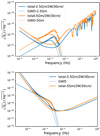Fig. 9

Upper panel: square root of the PSD noise TDI-X corresponding to different LISA configurations. The solid curves are the total PSD, while the dashed curves are the contribution from the confusion GWDs. The bundle of curves in the same colour corresponds to T_obs = 1, 2, 4, and 5 yr from top to bottom; Lower panel: sensitivity curves corresponding to different arm lengths and T_obs. The solid curves are the total curve, while the dashed curves are the contribution from the confusion GWDs. The bundle of curves in the same colour corresponds to T_obs = 1, 2, 4, and 5 yr from top to bottom.

4.2.2 Time-delay inference response to the SMBBH waveform

The TDI-X response of LISA to a GW from a SMBBH merger is calculated using the LDC code (Babak et al. 2010), where the IMRPhenomD waveform is adopted (Ajith et al. 2011). Figure 10 shows the modulus of the TDI-X responses in the frequency domain, for three different sources. The parameters of the example sources are listed in Table 2. The low-frequency limit corresponds to the time to coalescence at the beginning of the observation, and the dips at the high frequency end are due to the term sin(x) when converting to TDI. The sample cadence is fixed to 5 s, which corresponds to a high-frequency cut-off at 0.1 Hz. For systems with heavy BHs (masses >10⁵ M_⊙), such as #2 in the example, the frequency at coalescence is lower than the cut-off frequency, and therefore the current cadence will not lose any power from the signal; on the other hand, for systems with light BHs (masses < 50 000 M_⊙), as in #1 in the example, the high-frequency part (>0.1 Hz) of the waveform will be lost. However, the decrease in S/N is less than 1% compared to that using a cadence of 1 s. Therefore, it is acceptable to fix the cadence to 5 s for all sources in order to perform the simulation quickly.

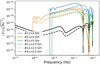Fig. 10

Modulus of frequency domain TDI-X responses to GWs from different SMBBHs (whose parameters are listed in Table 2). The solid curves correspond to LISA with 5 Gm laser arms, and dashed curves correspond to a 2.5 Gm arms configuration.

4.2.3 TDI waveform of DWD

We first derive the frequency domain TDI-X waveform in a monochromatic plane wave approximation. The equal-arm Michelson response of a plane GW in the long-wavelength region can be approximated as a sine wave with an orbitally averaged amplitude $〈 A 〉$ $\left\langle {\cal A} \right\rangle$ and frequency f_s. The relation between $〈 A 〉$ $\left\langle {\cal A} \right\rangle$ and the intrinsic amplitude A of the source binary can be found in Eqs. (A 12) and (A13) of Korol et al. (2017).

The Fourier transform of such a signal with the duration T_obs is: ${\tilde{h}}_{Mich} (f) = \frac{1}{2} 〈 A 〉 T_{obs} sinc ((f - f_{s}) T_{obs}) .$ ${S_{\rm{n}}} = {{10} \over {3{L^2}}}\left( {S_{{\rm{dis}}}^{{\rm{op}}} + 2\left( {1 + {{\cos }^2}\left( x \right)} \right){{S_{\rm{a}}^{{\rm{acc}}}} \over {{{\left( {2\pi f} \right)}^4}}}} \right)\left( {1 + {3 \over 5}{x^2}} \right) + {S_{{\rm{GWD}}}},$ (37)

We note that here we use the convention that sinc(x) = sin(πx)/(πx), such that the integration of ${| \tilde{h} (f) |}^{2}$ ${\left| {\widetilde h\left( f \right)} \right|^2}$ is equal to T_obsA²

To convert the equal-arm Michelson into TDI-X, we multiply by a factor 4x sin x, where x = f(2πL/с): $X (f) = 2 x \sin x 〈 A 〉 T_{obs} sinc ((f - f_{s}) T_{obs}) .$ ${\tilde h_{{\rm{Mich}}}}\left( f \right) = {1 \over 2}\left\langle {\cal A} \right\rangle {T_{{\rm{obs}}}}{\mathop{\rm sinc}\nolimits} \left( {\left( {f - {f_{\rm{s}}}} \right){T_{{\rm{obs}}}}} \right).$ (38)

Figure 11 shows the waveforms of a DWD with A = 10⁻²⁰ and f_s = 10⁻³ Hz calculated analytically from Eq. (38) compared to those calculated numerically with the LDC code (which is based on Cornish & Littenberg 2007). Although simplified, the overall agreement between the two is good.

From Eqs. (27) and (38), we obtain an approximated squared S/N expression: $ρ_{approx.}^{2} = \frac{16 x^{2} \sin^{2} x 〈 A^{2} 〉 T_{obs}}{S_{X} (f_{s})} .$ $X\left( f \right) = 2x\sin x\left\langle {\cal A} \right\rangle {T_{{\rm{obs}}}}{\mathop{\rm sinc}\nolimits} \left( {\left( {f - {f_{\rm{s}}}} \right){T_{{\rm{obs}}}}} \right).$ (39)

When we replace the TDI-X noise PSD with the Michelson noise PSD, and drop the 16x² sin² x term, the above equation becomes Eq. (10) of Korol et al. (2017).

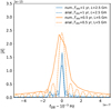Fig. 11

Frequency domain LISA responses to GW from a DWD: The blue and orange lines correspond to two different LISA configurations; solid and dashed lines correspond to responses calculated with numerical and analytical methods respectively.

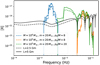Fig. 12

Frequency domain TDI-X responses to EMRI AK waveform, which correspond to three EMRI systems and two L designs of LISA.

Table 2

Parameters of example sources corresponding to Fig. 10.

4.2.4 TDI waveform for EMRIs

The analytic kludge (AK) waveforms (Barack & Cutler 2004) for EMRIs are applied and the corresponding TDI-X responses are calculated with the code package EMRI_Kludge_Suite⁴ (Chua & Gair 2015; Chua et al. 2017). As examples, Fig. 12 shows the frequency domain TDI-X responses to the AK waveforms, which correspond to three EMRI systems and two L designs of LISA. The first system (blue curves) has a SMBH with a mass of M = 10⁶ M_⊙ and a stellar-mass BH with a mass of m = 20 M_⊙. Here the masses are all measured in the frame of the observer, that is, they are all redshifted. The frequency domain response corresponds to a time-domain waveform simulated from the semi-latus rectum p = 8GM/c² to the final plunge. The time resolution is dt = 25 s, which is set to ensure that the highest frequency cut-off set by l/(2dt) is larger than the Kepler frequency around the innermost stable circular orbit (ISCO) of the SMBH. The lower frequency cut corresponds to the initial orbital inspirai, and the higher frequency cut corresponds to the orbital frequency at the plunge, which approximates to the Kepler frequency at ISCO; the second system (orange curves) has a SMBH with a mass of M = 10⁶ M_⊙ and a stellar mass BH with a mass of m = 20 M_⊙ The initial semi-latus rectum is also p = 8GM/c². As the Kepler frequency at ISCO is inversely proportional to the mass of the SMBH, we use dt = 2.5 s. The third system (green curves) is identical to the second one except for its initial semi-latus rectum, which is p = 20GM/c². To track the evolution from this larger initial semi-latus rectum to the final plunge, the simulation includes approximately 10 times longer time-steps. As a result, more low-frequency components are included in the third waveforms than in the second. Other physical parameters are identical for the three systems and are (values used in parenthesis) (Barack & Cutler 2004): s: dimension-less spin of the massive BH (s = 0.5); e: the initial eccentricity (e = 0); t: the initial inclination (t = 0.524 rad); y: the pericenter angle in AK Waveform (у = 0); ф: the initial phase (ф = 0.785 rad); ö_s: the sky position polar angle of a source in an ecliptic-based coordinate system, which is equal to л/2 minus the ecliptic latitude (ös = 0.785 rad); 0s: the sky position azimuth angle of a source in an ecliptic-based coordinate system, which is equal to the ecliptic longitude (<f>_s = 0.785 rad); Ö_K: the polar angle of the massive BH spin (Ö_K = 1.05 rad); фк- the azimuth angle of the massive BH spin (0_K = 1.05 rad); a: the azimuthal direction of the orbital angular momentum (a = 0); D: luminosity distance (D = 1 Gpc).

As mentioned above, if the frequency domain waveform were to be simulated in real time for every candidate event, it would be difficult to reconcile both the speed of the simulation and the inclusion of the full GW signal from the beginning of the observation to the plunge. As a solution, we generate the frequency domain TDI waveform corresponding to each candidate event in the catalogue in advance, and store their moduli in files. The pre-generated TDI waveform corresponds to the signal from the beginning of the observation to the final plunge. The initial semi-latus is calculated with the Newtonian formula Eq. (4.136) of Maggiore (2008) according to its mass, eccentricity, and time to plunge at the beginning of observation. The pre-calculated TDI corresponds to a LISA arm length of 2.5 Gm. The conversion to a different LISA arm length can be done by rescaling with x_1,i sin x_1,i/(x_0,i sin x_0,i) where: $x_{0, i} = 2 π f_{i} L_{default} / c,$ $\rho _{{\rm{approx}}{\rm{.}}}^2 = {{16{x^2}{{\sin }^2}x\left\langle {\,{{\cal A}^2}\,} \right\rangle {T_{{\rm{obs}}}}} \over {{S_X}\left( {{f_{\rm{s}}}} \right)}}.$ (40)

and $x_{1, i} = 2 π f_{i} L_{new /} c .$ ${x_{0,i}} = 2\pi {f_i}{L_{{\rm{default}}}}/c,$ (41)

4.3 PTAs

Pulsars are rotating neutron stars. Some of the known pulsars are very stable, that is, their spin period only changes by a tiny fraction over a very long epoch. Therefore, the arrival time of each pulse from such a pulsar can be modelled with high precision. The passing of a series of GWs will cause additional changes to the expected times of arrival (TOAs) of the pulses, which provides a way of detecting GWs at frequencies of between 10⁻⁸ and 10⁻⁵ Hz, where the lower frequency limit corresponds to the observation span of years, and the high frequency limit corresponds to the average cadence of a couple of days (see Sazhin 1978; Detweiler 1979; Hellings & Downs 1983; Jenet et al. 2005). A PTA is a group of pulsars that are stable and have been monitored with radio telescopes for a long time. The existing PTA consortia are EPTA (Kramer & Champion 2013), PPTA (Hobbs 2013), NANOGrav (McLaughlin 2013), and IPTA (Hobbs et al. 2010a). The standard procedure of pulsar timing is to first fit a timing model to the TOAs of individual pulsars, which includes inaccuracies in the astrometric parameters of the pulsars, a model for spin evolution, the refractive effects of interstellar medium and solar wind, the orbital and spin motion of the Earth, and delays due to general relativity (see Hobbs et al. 2006). The differences between the timing model and the observed TOAs, namely the timing residuals, are used to extract information about possible GW signals with frequentist (Jenet et al. 2005; Babak & Sesana 2012; Ellis et al. 2012) or Bayesian methods (van Haasteren et al. 2009; Ellis 2013). Here we want to use a simplified way to represent the properties of PTAs, without the need to make use of the full time-series of the timing residuals, and obtain results that agree to within an order of magnitude with the published results. We base our method on measuring the excess power from GW over analytic timing noise power spectra. Such an approach was also taken in some early studies (Jenet et al. 2004; Yardley et al. 2010; Yi et al. 2014).

4.3.1 Representing the timing noises

Supposing that we have already removed every known effect that contributed to differences in the TOAs, the timing residuals that remain are purely intrinsic to the pulsars and their spin irregularity. Previous studies found that such timing noise can be decomposed into a red noise component and a white noise component (Hobbs et al. 2010b). The red noise component can be represented with a power-law spectrum, with increasing power towards the lower frequencies, while the white noise component has a power level that is independent of frequency. In the GW-Toolbox, we use the following equation to represent the noise spectrum density of the timing residuals of an individual pulsar: $S_{total} (f) = σ_{w}^{2} / (f_{high} - f_{low}) + S_{n,red} (f),$ ${x_{1,i}} = 2\pi {f_i}{L_{{\rm{new}}/}}c.$ (42)

where σ_w is the level of the white noise, f_high = N/(2T) is the high frequency cut-off defined by the observation cadence, f_low = 1/T is the low frequency cut-off defined by the inverse of the duration, and S_n,red(f) is the red noise component, which has a power-law form: $S_{n.red} (f) = \frac{A_{red}^{2}}{12 π^{2}} {(\frac{f}{{yr}^{- 1}})}^{- α} .$ ${S_{{\rm{total}}}}\left( f \right) = \sigma _{\rm{w}}^2/\left( {{f_{{\rm{high}}}} - {f_{{\rm{low}}}}} \right) + {S_{{\rm{n,red}}}}\left( f \right),$ (43)

Therefore, we define the noise spectrum of a pulsar with five parameters, namely: N the number of observations, T the duration of observation, A_red the normalisation of the red noise, a the power index of the red noise, and σ_w the level of the white noise. The last three are intrinsic properties of the pulsar. These parameters for the pulsars in the above-mentioned PTAs are fitted and published (Desvignes et al. 2016; Porayko et al. 2019; Alam et al. 2021). The GW-Toolbox includes 42 pulsars in EPTA, 26 pulsars in PPTA, 47 pulsars in NANOGrav, and 87 pulsars in IPTA. Besides the pulsars in the current PTAs, the GW-Toolbox also includes simulated future observations with customised observation cadence and duration, and an increasing number of newly discovered pulsars during the observation period. The parameters (sky coordinates RA, Dec and noise parameters A_red, a, σ_w) of the simulated pulsars are assigned in the following way: randomly select two pulsars from the current PTA with replacement, and draw a uniformly random number between the parameters of the selected pair of pulsars, and assign the random variable as the corresponding parameter of the new pulsar. In this method, the noise properties and sky distribution of the new pulsars reflect those of the known pulsars.

In Fig. 13, we plot the noise spectra density of pulsars in the PTAs used by the GW-Toolbox. Figure 14 shows the sky coordinates of pulsars in the PTA.

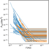Fig. 13

Noise spectra of the pulsars. Blue curves correspond to known pulsars in existing PTAs, and orange curves are simulated new pulsars.

4.3.2 PTA detections

The GW from an individual SMBH can be approximated with a monochromatic wave. The timing residuals induced in the ith pulsar are (Yi et al. 2014): $A_{i} = \frac{h_{s}}{w} (1 + \cos θ) \sqrt{\cos^{2} 2 ψ (\frac{1 + \cos^{2} l}{2}) + \sin^{2} 2 ψ \cos^{2} l,}$ ${S_{{\rm{n}}{\rm{.red}}}}\left( f \right) = {{A_{{\rm{red}}}^2} \over {12{\pi ^2}}}{\left( {{f \over {{\rm{y}}{{\rm{r}}^{ - 1}}}}} \right)^{ - \alpha }}.$ (44)

where θ, ι, and Ψ are the angle between the direction towards the pulsar and the GW source, the inclination of the source binary plan, and the polarization angle, respectively. The S/N of the GW in the ith pulsar is: $ρ_{i}^{2} = A_{i}^{2} / S_{n, i} (f) \times T_{i},$ ${{\cal A}_i} = {{{h_s}} \over w}\left( {1 + \cos \theta } \right)\sqrt {{{\cos }^2}2\psi \left( {{{1 + {{\cos }^2}l} \over 2}} \right) + {{\sin }^2}2\psi {{\cos }^2}l,}$ (45)

where S_n,i(f) is the noise spectrum density of the pulsar, and T_i is the observation duration. The total S/N squared of a PTA is: $p^{2} = \sum ρ_{i}^{2} .$ $\rho _i^2 = {\cal A}_i^2/{S_{n,i}}\left( f \right) \times {T_i},$ (46)

The effects of SGWB on the timing residual are an additional red noise: $h_{c}^{2} (f) = C f^{γ},$ ${p^2} = \sum {\rho _i^2.}$ (47)

where h_c is the characteristic GW strain at the frequency of lyr⁻¹, and the index γ depends on the origin of the SGWB. For incoherent overlapping of MBH, γ = −2/3; for relic GW, γ = −1; and for cosmic strings, γ = −7/6. Besides the additional red noise, the timing residuals due to the SGWB are also expected to be correlated between pairs of pulsars. The correlation as a function of the angular separation between the pair is: $Γ_{0} = 3 {\frac{1}{3} + \frac{1 - \cos ξ}{2} - [\ln (\frac{1 - \cos ξ}{2} - \frac{1}{6}]},$ $h_{\rm{c}}^2\left( f \right) = C{f^\gamma },$ (48)

which is referred to as the Hellings and Downs curve (Hellings & Downs 1983). The S/N squared in a pair of pulsars is (Anholm et al. 2009): $ρ_{1, 2} = \frac{H_{0}^{2}}{4 π^{2}} \sqrt{2 T \int_{0}^{\infty} d f \frac{Ω_{gw}^{2} (f) Γ_{0}^{2}}{f^{6} p_{1} (f) p_{2} (f)},}$ ${{\rm{\Gamma }}_0} = 3\left\{ {{1 \over 3} + {{1 - \cos \xi } \over 2} - \left[ {\ln ({{1 - \cos \xi } \over 2} - {1 \over 6}} \right]} \right\},$ (49)

where H₀ is the Hubble constant, and Ω_gw(f) is the energy density of the SGWB relative to the critical density of the Universe. The relation between h_c(f) and Ω_gw(f) is: $h_{c}^{2} (f) = \frac{3 H_{0}^{2}}{2 π^{2}} \frac{1}{f^{2}} Ω_{gw} (f) .$ ${\rho _{1,2}} = {{H_0^2} \over {4{\pi ^2}}}\sqrt {2T\mathop \smallint \limits_0^\infty {\rm{d}}f{{{\rm{\Omega }}_{{\rm{gw}}}^2\left( f \right){\rm{\Gamma }}_0^2} \over {{f^6}{p_1}\left( f \right){p_2}\left( f \right)}},}$ (50)

In Eq. (49), P_1,2(f) = S_n1,2(f)f² The total S/N squared is the summation of the S/N squared over all pairs in the PTA.

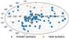Fig. 14

Galactic distribution of the PTAs. The blue dots indicate the pulsars from current IPTA, and the orange dots indicate the simulated new pulsars. The size of the markers is proportional to the number of TOAs of the corresponding pulsar.

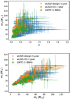Fig. 15

Simulated catalogue vs. catalogue from real observations: aLIGO-design-1 year: simulated catalogue from 1 yr of observation by aLIGO with designed noise performance on BBH, marked with blue crosses; aLIGO-O3-1 yr: simulated catalogue from 1 yr of observation by aLIGO with O3 noise performance on BBH, marked with orange dots; GWTC-3 (BBH): BBH events in GWTC-3, marked with green star symbols.

5 Results and examples

In order to test and validate the GW-Toolbox, we discuss the outcome of the simulations for the different source populations and different detectors, and compare these with findings in the literature where possible.

5.1 Examples for stellar-mass BBH detected with Earth-based detectors

For BBHs, we generate catalogues for a one-year observation of aLIGO, both with the noise spectrum of O3 (aLIGO-O3) and that of the design (aLIGO-design). The underlying population model is BBH-PopB with the default parameters (delay time of 3 Gyr and a mass function with an extra Gaussian peak at 40 M_⊙; see Sect. 3.1.1). The simulated number of detections by aLIGO-O3 is 99 (with a Poisson expectation 87.4), which is compatible with the rate of detection in ОЗа (~36 BBH in six months of observation with a duty cycle of ~80%, see Abbott et al. 2020c); the simulated number of detections for the aLIGO-design is 379 (expectation 376.0). In the panels of Fig. 15, we plot the simulated catalogues in the z−m₁ and m₁ − m₂ planes. To compare, we also plot the BBH events in GWTC-3 (Abbott et al. 2021b), which is comprised of GWTC-1 (Abbott et al. 2019b) and events detected in O3a+b. The simulated sets agree well with the observed ones, except that the uncertainties on parameters are in general larger in our simulation than those in the real observation in GWTC-3 (up to ~50%), especially in the low-S/N region. The origin of this overestimation is two-fold: (1) the intrinsic difference between FIM and Bayesian methods, as mentioned above; and (2) the localisation information from triangulation is not included in our method as it was in the real catalogue. Therefore, the estimated uncertainties can serve as conservative upper limits.

We also simulate a catalogue of one month of observation with ET. In this case, the number of detections is 1923 (expectation 1.9 × 10³). In the panels of Fig. 16, we plot the distribution of the catalogue in z and m₁. We also plot the distribution of BBH mergers in the whole Universe as defined by the population model for comparison. From this example, it is clear that ET will probe the distribution of sources throughout the Universe very well, as was shown before (e.g. Vitale & Evans 2017). We will study this in more detail in a forthcoming paper (Yi et al. 2022)

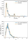Fig. 16

m₁ distribution (upper panel) and the number density as function of redshift (lowerpanel) in the catalogue for 1 month of observation of BBH mergers by ET (solid blue line). The integral of the latter is the total number of detections. As a comparison, we plot the distribution of BBH mergers for the whole Universe within 1 month (dashed orange line).

5.2 Exampies for DNSs detected with Earth-based detectors

The number of DNS mergers detected so far is small (2–3). Therefore, we generate catalogues for 10 yr of detection of DNS mergers by aLIGO, both with the noise spectrum in O3 (aLIGO-O3) and that in design (aLIGO-design). The number of detections by aLIGO-O3 is 56 (expectation 48.7) in 10 yr, which is in accordance with the real detection rate in ОЗа (1–2 in 6 months); the number for aLIGO-design is 238 (expectation 236.3). Figure 17 shows the simulated catalogues in the z − m₁ and m₁ – m₂ planes. We also plot the DNS events in GWTC-3 (GW170817, GW190425) for comparison. It is difficult to draw strong conclusions with so few detections, but broadly the results of the GW-Toolbox agree with the observations so far. To look further into the future, we also simulate the catalogue of 1 yr of observation with ET. The expected number of detections is 168 455 (expectation 1.68 × 10⁵). Figure 18 shows the distribution of the catalogue in redshift and total mass. We also plot the distribution of DNS mergers in the whole Universe as defined by the population model for comparison. As we can see from the upper panel of Fig. 18, the detected mass distribution is shifted to the high-mass side due to higher detectability; and in the lower panel of Fig. 18, we see the portion of detectable DNS mergers decreases towards higher redshift, as expected.

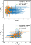Fig. 17

The same as Fig. 15, but for 10 yr observation of DNS with eLIGO (design and O3 sensitivity).

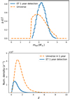Fig. 18

Total mass distribution (upperpanel) and the number density as functions of redshift (right panel) in the catalogue of 1 yr of observation of DNS mergers by ET (solid blue). The integral of the latter is the total number of detections. The dashed orange curve is the same but for the whole Universe within 1 yr.

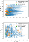Fig. 19

As in Fig. 15 but with BHNSs: aLIGO-design-10yr: simulated catalogue from 10 yr of observation by aLIGO with designed noise performance on BHNSs, marked with blue crosses; aLIGO-O3-10 yr: simulated catalogue from 10 yr of observation by aLIGO with O3 noise performance on BHNS, marked with orange dots.

5.3 Example for BHNS mergers detected with Earth-based detectors

In a similar way to above, we generate catalogues for 10 yr of aLIGO observations for BHNS mergers, both with the noise spectrum in O3 (aLIGO-O3) and that in design (aLIGO-design). The underlying population model is BHNS-PopB with the default parameters. The event number in the simulated catalogue of aLIGO-O3 is 29 (a Poisson random with expectation value 32.0), which is compatible with the rate found in the O3 period (2–3 in 1 yr); the number for aLIGO-design is 553 (expectation value 517.2). The top and bottom panels of Fig. 19 show the simulated catalogues in z − m_● and m_● − m_n planes. A more sensitive detector would help to properly characterise this population.

We also simulate a catalogue for 1 yr of observation by ET. The number of events is 6251 (expectation 6.32 × 10⁴). Figure 20 shows the distribution of the catalogue in z, m_●, and m_n. We also plot the distribution of BHNS mergers in the whole Universe as defined by the population model for comparison. We see that the fraction of detectable BHNS mergers increases towards higher masses, and decreases towards higher redshift, although ET probes essentially the whole distribution.

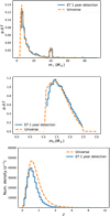Fig. 20

Probability density distribution as a function of m_● (upper panel) and m_n (middle panel), and number density as a function of red-shift (lower panel) for 10 yr of observation of BHNS mergers by ET. The integral of the latter is the total number of detections. The orange lines show the intrinsic distributions.

5.4 Examples for SMBBH mergers detected with LISA

We now turn to the space-based detectors. The GW-Toolbox simulates the observed catalogue of SMBBH mergers by going through the catalogue in the Universe for a given observation duration, calculates the S/N for each SMBBH, and selects against the S/N cut-off; in this case S/N = 8 as default. In Fig. 21, we plot the redshifted chirp masses and the redshift of the total events and detected ones (squares on top of markers) by the standard LISA configuration in 5 yr, corresponding to different population models. As we can see from Fig. 21, the detection horizon of our default LISA passes though the РорЗ population and below the Q3_delays and Q3_nodelays populations. As a result, almost all events in Q3_delays and Q3_nodelays population are detectable, while the detectable fraction of РорЗ changes significantly with different LISA noise settings.

For these sources, we also calculate the uncertainties on the parameters. Figure 22 shows the distribution of the relative uncertainties on total mass, distance, and sky localisation dΩ in units of square degrees. The uncertainties are all estimated with a FIM method. The uncertainties span a wide range, but a significant fraction have relatively well-determined masses while only a small fraction have well-determined distance and sky position. Our findings agree in general with previous results of Klein 16.

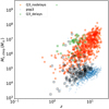Fig. 21

Redshifted chirp masses and the redshift of the total events (markers) and detected ones (squares on top of markers) by the standard LISA configuration in 5 yr. Orange, blue, and green markers correspond to Q3_nodelay, рорЗ, and Q3_delays population models, respectively. The underlying S/N cutoff is 8.

Table 3

Detection of the verification binaries with the LISA detector.

5.5 Examples for DWDs detected with LISA

In order to simulate the DWDs observed by LISA, we go through a simulated catalogue of all Galactic DWDs and calculate their S/N with the analytic approximation in Eq. (39). We then select the sources with S/N larger than the S/N threshold of 10 as the detected sources. We do the same for the VBs. In Table 3, we list the detected VBs and the estimated uncertainties on the parameters. When calculating the uncertainties with FIM, the numerical waveform calculated with LDC is used. The results are compatible with those of earlier studies, and the S/N is slightly lower than that of Kupfer et al. (2018) because of the use of a slightly different LISA sensitivity. As the DWD catalogue is very large (~2.6× 10⁷), we go through a smaller subcatalogue that is randomly drawn from the whole synthetic DWD catalogue instead, and scale the number of detections from this small subsample to the whole GWD catalogue to obtain the total expected number of detections. Figure 23 shows the number of detections as a function of the observation duration. The number of detections we find is about a factor of 0.5 lower than the number found in earlier studies; for example those of Nelemans et al. (2001), Nissanke et al. (2012), Korol et al. (2017). We attribute this to a slight difference in the LISA noise model or the DWD catalogue.

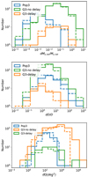Fig. 22

Distributions of relative uncertainties and the uncertainties of the sky location of the events in the simulated catalogue: Upper: distribution of relative uncertainties on the total masses in the catalogue of SMBBH mergers detected by LISA in 5 yr. Solid lines are for default LISA and dashed lines are for 5 Gm arm length. Middle: same as the upper panel, but on the relative uncertainties on the luminosity distances. Lower: same as the upper two panels, but on uncertainties of the sky location (deg²).

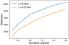Fig. 23

Detected number of DWDs with the default LISA and a larger LISA with 5 million km arms as a function of the observation duration. We use a threshold S/N ρ_⋆ = 7.

Table 4

Upper limits set with different PTAs to SGWB of different origins, ρ_cri = 100.

5.6 Examples for EMRIs detected with LISA

The signal from an EMRI can fall into the detectable frequency range of LISA from an early phase until the final plunge, which can span quite a long duration from months to years. In order to guarantee the speed of simulation, we use a frequency domain waveform (modulus) generated in advance and stored in files. In each simulation, we go through all the candidate events in the catalogue, read in the corresponding TDI waveform modulus, and calculate the S/N against the noise curve. The detected events are then selected against an S/N threshold. In the EMRI catalogues that we are using, there is also a pre-calculated S/N for each system, which corresponds to a slightly different LISA setup and waveform (see Babak 17). In Fig. 24, we compare their pre-calculated S/Ns with ours of the same catalogue for 1 yr of observation of the M1 population with our default LISA. Our calculated S/N values disperse within a factor two around the values of Babak 17. We attribute this dispersion to the slightly different LISA noise and waveform (AK Schwarzchild versus AK Kerr, see Babak 17). In Fig. 25, we plot the histogram of the S/N of the bright EMRIs in the catalogue of Babak 17 and that calculated from this work. The underlying population model is M1. Figure 26 shows histograms of the relative uncertainties of the masses μ, M, distance D, and sky location Ω (in units of square degrees) in a catalogue detected by the default LISA. The observation duration is two years, the S/N cut-off is set to 20, and the population is M1. The uncertainties are estimated with FIM (Sect. 4.1.2). In the calculation of FIM, derivatives of the complex waveform relative to all the relevant parameters are needed (Eq. (25)). Therefore, if we were to use the pre-calculated waveform for the uncertainty estimation, the storing files would be about 20 times larger in size than those used for the S/N calculation. On that account, we calculate the late stage waveform in real time and use them for the uncertainty evaluation. In general, the parameters of EMRIs are very well determined, except for the sky position in some cases. The estimated levels of uncertainty are in agreement with those of Babak17.

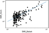Fig. 24

Pre-calculated S/N by Babak 17 compared to the S/N of this work for the same catalogue, for 1 yr of observation of the Ml population.

5.7 Results for pulsar timing arrays

For PTAs, we calculate the detection limits for individual SMBBHs and a stochastic background based on the different PTA configurations. Given a certain PTA, a S/N cut-off and the coordinates of the source, we can obtain a sensitivity curve for GWs emitted by an individual SMBBH as a function of frequency. Figure 27 shows the sky-averaged sensitivity curve to individual sources of EPTA, PPTA, NANOGrav, IPTA, and a simulated future PTA (labelled ‘future’). For the future PTA, we assume a daily observation of the IPTA pulsars for a further 10 yr, with two more new pulsars being added to the PTA per year (the setting of the future PTA can be customised by users). The corresponding ρ_cri = 10. The results are in agreement with others from the literature (Babak et al. 2016; Schutz & Ma 2016; Aggarwal et al. 2019).

In Table 4, we list the upper limits on the SGWB of different origins; the corresponding ρ_cri = 100. They are broadly in agreement with published results (to within a factor ~2), which are also provided in parentheses in the table.

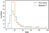Fig. 25

Histogram of the SNR of the bright EMRIs in catalogue of BabaklX The blue histogram indicate the SNR calculated in this work, and the orange histogram is that pre-calculated by Babak17 using a slightly different LISA noise and waveform.

6 Caveats and discussion

We implement and describe a first version of the GW-Toolbox, which still has a few caveats and is missing some ingredients that we plan to implement in the (near) future. The most important caveats of the current version are:

Higher order multipole modes of the waveform: Theoretically, GW radiation is treated with spin-weighted spherical decomposition (Thorne 1980). The leading term is the ℓ = 2, |m| = 2 (quadrupole) term. In the current GW-Toolbox, we apply a waveform that neglects the higher order modes beyond quadrupole. High-order modes will extend the spectrum of a GW to high frequencies (London et al. 2018), and their significance increases with higher mass inequality, higher total mass, and higher orbital inclination angle (Mills & Fairhurst 2021). Including higher order modes in the waveform can break the degeneracy between inclination angle and distance, and therefore results in more accurate estimates of the parameters of the source (London et al. 2018). In the O3 observation, there are already some GW events with evidence of higher order modes (GW170729: Chatziioannou et al. 2019; GW190412: Abbott et al. 2020b; GW190814: Abbott et al. 2020d). Mills & Fairhurst (2021) found that a few percent of binaries will be detected with higher order modes by aLIGO with designed sensitivity. For 3G GW detectors, Divyajyoti et al. (2021) found that the S/N contribution from higher order modes in some GWTC-3 systems would surpass 10% of the total S/N. For larger total mass and mass-ratio binaries, the higher order modes are expected to contribute a significant fraction of the S/N. Therefore, neglecting higher order modes in the waveform will result in underestimation of the detection rate of sources, especially for those with large total mass and mass ratio. In an updated GW-Toolbox, the waveform will be replaced with one that includes the higher order modes; for example PhenomHM (London et al. 2018).
Estimation of uncertainties for Earth-based detectors: The uncertainties are estimated in a hybrid way. Those of the intrinsic parameters (m_i,z and χ) are calculated with FIM, with all of the amplitude parameters treated as one. In addition, the uncertainty on the redshift (δz) is estimated with empirical relations. The source-frame mass uncertainties are then calculated with an error propagation (Eq. (26)). Equation (26) is valid only when the covariance between dm_i,z and dz vanishes. As m_i,z are largely determined from matching the phases of the waveform, while the constraint on z comes from the fitting amplitude of the waveform, we expect that the dependence between dm_i,z and dz is weak. A more self-consistent and accurate non-Bayesian treatment would be to treat all extrinsic parameters separately in the FIM (the dimension of FIM would thus be enlarged), and calculate the covariance among all parameters explicitly. The constraints from the triangulation localization could then be imposed in order to obtain the uncertainties on all parameters.
Populations and waveforms of EMRIs: In order to return the simulated catalogue of detection within a workable time-frame for the user of the website, we use catalogues of EMRIs in which only bright ones are included (pre-calculated S/N_tot > 20). Therefore, the user should not set an S/N cut-off lower than ~15; otherwise, the returned synthetic catalogue is incomplete. In order to compare with previous results of Babak17, the waveform we employed is analytic kludge, which is known to be fast but less realistic than others. In the GW-Toolbox, it can easily be replaced with a more accurate waveform, namely augmented analytic kludge (AAK), as the latter can also be simulated with the same package EMRI_Kludge_Suite. For the sake of the speed of simulation, we use the pre-calculated frequency domain TDI waveform for the S/N calculation. When estimating the uncertainties on parameters for the detected sources using FIM methods, we only include the late stage of their waveform. As shown in the above sections, we miss some of the low-frequency section corresponding to the early inspirai stage, which is in fact detectable by LISA, and results in underestimation of the accuracy of parameter inference. As shown in examples in the above section, such underestimation is not severe.
PTAs: our sensitivity curves and upper limits are given according to an S/N threshold and the S/Ns of GWs are calculated based on a simplified parameterised noise spectrum. On the other hand, upper limits are reported in the literature with confidence levels. Due to the very different natures of these two methods, the correspondence between the confidence level from the literature and our S/N threshold is difficult to explore. In our examples, we set ρ_cri = 10 for continuous GWs when plotting the sensitivity curves, and ρ_cri = 100 for SGWB in order to obtain results that are within the same order of magnitude of the results in the literature. For continuous GWs, the sensitivity scales with ρ_cri; while for SGWB, upper limits on the characteristic strain scale with the square root of ρ_cri.

We plan to include a number of additions to the GW-Toolbox in the future. The first ones involve several proposed space-borne detectors, in particular DECIGO, Taiji, and Tianqin. In the ground-based and space-borne modules, we will integrate S/N calculators for individual sources that are specified by the user. On a longer timescale, we plan to include more GW sources, such as supernovae explosions, single spinning and recycling neutron stars, multiple black hole encounters, and catalogues of SMBBHs for PTAs. We are also working to extend the GW-Toolbox with electro-magnetic counterparts, for example to return the fluence of short GRBs and peak fluxes of kilonovae. Triangulation of a network of ground-based detectors will also be developed.

In the next step, the GW-Toolbox will have the ability to simulate observations of different evolutionary phases of the same population in different GW frequency ranges. For instance, each population of compact object mergers corresponds to a population of persistent GW sources from the earlier phase. The former are targets of ground-based interferometers, while the latter are targets of space-borne interferometers. Another instance is the close orbit and inspiral-merger phases of SMBBHs, which can be observed with PTAs and LISA, respectively. We will also include simulated observation of the SGWB with ground-based and LISA-like detectors.

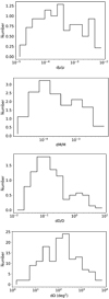Fig. 26

Histogram of relative uncertainties on the mass of the lighter component μ, the mass of the heavier component M, and the distance D, and the uncertainties on the sky location dΩ. in a catalogue of EMRIs detected by the default LISA for two years of observation. The S/N cutoff is setto 20.

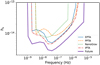Fig. 27

Sensitivity plot for an individual SMBBH as a function of frequency for ρ_cri = 10 and averaged over the celestial sphere for different PTAs.

7 Summary

In this paper, we introduce the GW-Toolbox⁵, a set of tools that quickly simulates a Universe with kHz, mHz, and nHz GW source populations, and observations with different GW detectors, that is, ground-based interferometers, space-borne interferometers, and PTAs. The functionalities and methodologies of the GW-Toolbox for each module can be summarised as follows:

The module for ground-based interferometers simulates observation of mergers of compact objects, including BBHs, DNSs, and BHNSs. The detectors include default aLIGO, Virgo, KAGRA, ET, and CE, and user-customised LIGO/Virgo-like and ET-like detectors. The noise curves of the default detectors are taken from the literature, and those of user-customised detectors are simulated with the FINESSE software. After the noise curve and antenna patterns are determined, we calculate the optimal S/N for all sources in the selected source class. A simplified IMRPhenomD waveform that assumes zero effective spin is employed in this step. With a certain S/N threshold of detection, we marginalise the geometrical parameters and obtain the detectability $D (m_{1}, m_{2}, z, χ)$ ${\cal D}\left( {{m_1},{m_2},z,\chi } \right)$ as a function of the mass, red-shift, (luminosity distance) and effective spin of the source. The product of $D (m_{1}, m_{2}, z, χ)$ ${\cal D}\left( {{m_1},{m_2},z,\chi } \right)$ and the user-selected probability density function (PDF) of the source population defines the PDF of the detectable sources, N_d(m₁, m₂, z, χ). A synthetic catalogue of observations is obtained with a MCMC sampling from the N_d(m₁, m₂, z, χ). We use a FIM method to estimate the uncertainties on the parameters of events. In the process of calculating the FIM, we apply the complete IMRPhenomD waveform phases (for aligned spins).
The module for space-borne interferometers simulates observations with LISA or a customised LISA-like configuration. The noise power density in the TDI-X response channel is calculated with an analytical formula, which includes acceleration noise, laser shot noise, other optical meteorology noises, and confusion noise due to Galactic DWD foreground. The targets we include are the inspiral of SMBBHs, individual resolvable Galactic DWDs and EMRIs. For SMBBHs, we calculate the TDI-X LISA responses of a GW source with LDC codes. The optimal S/N is subsequently calculated. We considered three population models, namely Pop3, Q3_nodelays, and Q3_delays, taken from Babak17, and performed ten realisations of the simulated catalogues of SMBBH mergers in the Universe within 5 yr for each population model. The GW-Toolbox will re-sample from the catalogue according to user specified observation duration, and calculate the S/N for each source in the sample. A synthetic detection catalogue is thus returned based on a S/N threshold of detection set by the user. The uncertainties are estimated with FIM. For DWDs, we use an analytic equation to calculate the modulus TDI-X LISA response to a series of sinusoidal GWs, and therefore the S/N. We consider two samples of DWDs, namely the verification DWDs and a simulated entire Galactic population. For the former sample, the S/N is calculated individually in the catalogue, and a detected catalogue is returned according to a S/N threshold. For the latter sample, due to its vast size, we randomly draw a subsample from it, and find the catalogue of detections in the subsample. The total expected number of detections is obtained by rescaling the number of events in the returned catalogue. The uncertainties are also estimated with FIM, where we use LDC codes for the complex TDI LISA response instead of using the analytical equation as in the S/N computation. For EMRIs, we make use of the EMRI_Kludge_Suite for the TDI LISA response, and therefore the S/N. We calculate the S/N for each source in pre-simulated catalogues of EMRIs of different populations, and select those with S/N surpassing the S/N threshold. The uncertainties are again computed with FIM.
In the PTA module, we include four currently operating PTAs: EPTA, PPTA, NANOGrav, and IPTA. For the pulsars in these PTAs, we use the following parameters to represent their noise properties and observation campaigns: the levels of white noise, the level of red noise, the red noise spectrum index, total observation duration, and the average interval between observations. We allow users to include new pulsars that will be discovered in the course of future observations. The sky locations of the new pulsars and their noise properties are randomly assigned according to the distributions of those of the known pulsars. In this module, the GW-Toolbox computes the S/N of a series of monochromatic GWs with given frequency and amplitude, which corresponds to a GW from the orbital motion of a SMBBH. Another function of this module is to evaluate the upper limit that a PTA can set on the stochastic GW background from different origins.

In the (near) future, the GW-Toolbox will be extended with new standard detectors, triangulation of a network of ground-based detectors, new source classes and electro-magnetic counterparts, and the ability to ‘observe’ the same source model with different detectors. In this way, the GW-Toolbox will provide even more functionality to give users a quick idea of the power of different GW detectors for their favourite source population.

Acknowledgements

We thank the many researchers that provided results for the different source populations and detectors that made it possible to collect all these together in the GW-Toolbox. We also thank the referee for comments and detailed testing that greatly improved the paper and the GW-Toolbox. We thank in particular the (Mock) LISA Data Challenge team and the participating groups that made it possible to include so many results in the space module. Special thanks to Stas Babak and Antoine Petiteau for help and support. We thank our colleagues Paul Groot, Samaya Nissanke, Sarah Caudill, Chris van den Broeck, Gemma Janssen, Antonia Rowlinson, Peter Jonker, Selma de Mink, Marc Klein-Wolt and Jess Broderick for the initial discussions that led to this project. This research was made possible by support from the Dutch National Science Agenda, NWA Startimpuls – 400.17.608.

Appendix A Conversion from one LISA response to another

In the above sections, when working with LISA responses to GW signal and noise, we often need to convert one kind of LISA response to another. We summarise the conversion relationship in figure A.1.

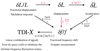Fig. A.1

Conversion between different kinds of LISA responses

References

Abbott, B. P., Abbott, R., Abbott, T. D., et al. 2016a, Phys. Rev. Lett., 116, 061102 [Google Scholar]
Abbott, B. P., Abbott, R., Abbott, T. D., et al. 2016b, ApJ, 818, L22 [Google Scholar]
Abbott, B. P., Abbott, R., Abbott, T. D., et al. 2017a, Phys. Rev. Lett., 119, 161101 [Google Scholar]
Abbott, B. P., Abbott, R., Abbott, T. D., et al. 2017b, ApJ, 848, L12 [Google Scholar]
Abbott, B. P., Abbott, R., Abbott, T. D., et al. 2017c, ApJ, 848, L13 [CrossRef] [Google Scholar]
Abbott, B. P., Abbott, R., Abbott, T. D., et al. 2017d, Nature, 551, 85 [Google Scholar]
Abbott, B. P., Abbott, R., Abbott, T. D., et al. 2017e, ApJ, 850, L39 [NASA ADS] [CrossRef] [Google Scholar]
Abbott, B. P., Abbott, R., Abbott, T. D., et al. 2017f, ApJ, 850, L40 [NASA ADS] [CrossRef] [Google Scholar]
Abbott, B. P., Abbott, R., Abbott, T. D., et al. 2018a, Phys. Rev. Lett., 121, 161101 [Google Scholar]
Abbott, B. P., Abbott, R., Abbott, T. D., et al. 2018b, Phys. Rev. Lett., 120, 091101 [CrossRef] [Google Scholar]
Abbott, B. P., Abbott, R., Abbott, T. D., et al. 2019a, Phys. Rev. X, 9, 011001 [Google Scholar]
Abbott, B. P., Abbott, R., Abbott, T. D., et al. 2019b, Phys. Rev. X, 9, 031040 [Google Scholar]
Abbott, B. P., Abbott, R., Abbott, T. D., et al. 2019c, Phys. Rev. Lett., 122, 061104 [NASA ADS] [CrossRef] [Google Scholar]
Abbott, B. P., Abbott, R., Abbott, T. D., et al. 2019d, Phys. Rev. Lett., 123, 011102 [Google Scholar]
Abbott, B. P., Abbott, R., Abbott, T. D., et al. 2019e, ApJ, 882, L24 [Google Scholar]
Abbott, B. P., Abbott, R., Abbott, T. D., et al. 2020a, Class. Quant. Grav., 37, 045006 [NASA ADS] [CrossRef] [Google Scholar]
Abbott, R., Abbott, T. D., Abraham, S., et al. 2020b, Phys. Rev. D, 102, 043015 [NASA ADS] [CrossRef] [Google Scholar]
Abbott, R., Abbott, T. D., Abraham, S., et al. 2020c, Phys. Rev. X 11, 021053 [NASA ADS] [Google Scholar]
Abbott, R., Abbott, T. D., Abraham, S., et al. 2020d, ApJ, 896, L44 [Google Scholar]
Abbott, R., Abbott, T. D., Abraham, S., et al. 2021a, ApJ, 915, L5 [NASA ADS] [CrossRef] [Google Scholar]
Abbott, R., Abbott, T. D., Acernese, F., et al. 2021b, https://dcc.ligo.org/public/0170/P2000318/007/o3b_catalog.pdf [Google Scholar]
Abbott, R., Abbott, T. D., Abraham, S., et al. 2021c, ApJL, 913, L7 [NASA ADS] [CrossRef] [Google Scholar]
Acernese, F., Agathos, M., Agatsuma, K., et al. 2015, Class. Quant. Grav., 32, 024001 [Google Scholar]
Aggarwal, K., Arzoumanian, Z., Baker, P. T., et al. 2019, ApJ, 880, 116 [NASA ADS] [CrossRef] [Google Scholar]
Aggarwal, K., Arzoumanian, Z., Baker, P. T., et al. 2020, ApJ, 889, 38 [NASA ADS] [CrossRef] [Google Scholar]
Aggarwal, N., Aguiar, O. D., Bauswein, A., et al. 2021, Liv. Rev. Relat., 24, 4 [NASA ADS] [CrossRef] [Google Scholar]
Ajith, P., Hannam, M., Husa, S., et al. 2011, Phys. Rev. Lett., 106, 241101 [NASA ADS] [CrossRef] [Google Scholar]
Alam, M. F., Arzoumanian, Z., Baker, P. T., et al. 2021, ApJS, 252, 5 [Google Scholar]
Amaro-Seoane, P., Gair, J. R., Freitag, M., et al. 2007, Class. Quant. Grav., 24, R113 [NASA ADS] [CrossRef] [Google Scholar]
Amaro-Seoane, P., Audley, H., Babak, S., et al. 2017, Arxiv e-prints [arXiv:1702.00786] [Google Scholar]
Anholm, M., Ballmer, S., Creighton, J. D. E., et al. 2009, Phys. Rev. D, 79, 084030 [NASA ADS] [CrossRef] [Google Scholar]
Antoniadis, J., Arzoumanian, Z., Babak, S., et al. 2022, MNRAS, 510, 4873 [NASA ADS] [CrossRef] [Google Scholar]
Armstrong, J. W., Estabrook, F. B., & Tinto, M. 1999, ApJ, 527, 814 [NASA ADS] [CrossRef] [Google Scholar]
Arzoumanian, Z., Baker, P. T., Brazier, A., et al. 2018, ApJ, 859, 47 [NASA ADS] [CrossRef] [Google Scholar]
Arzoumanian, Z., Baker, P. T., Blumer, H., et al. 2020, ApJ, 905, L34 [NASA ADS] [CrossRef] [Google Scholar]
Astropy Collaboration (Robitaille, T. P., et al.) 2013, A&Amp;A, 558, A33 [NASA ADS] [CrossRef] [EDP Sciences] [Google Scholar]
Astropy Collaboration (Price-Whelan, A. M., et al.) 2018, AJ, 156, 123 [Google Scholar]
Babak, S., & Sesana, A. 2012, Phys. Rev. D, 85, 044034 [NASA ADS] [CrossRef] [Google Scholar]
Babak, S., Baker, J. G., Benacquista, M. J., et al. 2010, Class. Quant. Grav., 27, 084009 [NASA ADS] [CrossRef] [Google Scholar]
Babak, S., Petiteau, A., Sesana, A., et al. 2016, MNRAS, 455, 1665 [NASA ADS] [CrossRef] [Google Scholar]
Babak, S., Gair, J., Sesana, A., et al. 2017, Phys. Rev. D, 95, 103012 [NASA ADS] [CrossRef] [Google Scholar]
Barack, L., & Cutler, C. 2004, Phys. Rev. D, 69, 082005 [NASA ADS] [CrossRef] [Google Scholar]
Barausse, E. 2012, MNRAS, 423, 2533 [NASA ADS] [CrossRef] [Google Scholar]
Barausse, E., Berti, E., Hertog, T., et al. 2020, Gen. Relat. Grav., 52, 81 [CrossRef] [Google Scholar]
Barke, S., Wang, Y., Esteban Delgado, J. J., et al. 2015, Class. Quant. Grav., 32, 095004 [NASA ADS] [CrossRef] [Google Scholar]
Belczynski, K., Kalogera, V., & Bulik, T. 2002, ApJ, 572, 407 [NASA ADS] [CrossRef] [Google Scholar]
Belczynski, K., Holz, D. E., Bulik, T., et al. 2016, Nature, 534, 512 [NASA ADS] [CrossRef] [Google Scholar]
Berti, E., Cardoso, V., & Will, C. M. 2006, Phys. Rev. D, 73, 064030 [NASA ADS] [CrossRef] [Google Scholar]
Brown, D. D., Jones, P., Rowlinson, S., et al. 2020, SoftwareX, 12, 100613 [NASA ADS] [CrossRef] [Google Scholar]
Burke-Spolaor, S., Taylor, S. R., Charisi, M., et al. 2019, A&Amp;A Rev., 27, 5 [Google Scholar]
Caprini, C., & Figueroa, D. G. 2018, Class. Quant. Grav., 35, 163001 [NASA ADS] [CrossRef] [Google Scholar]
Chatziioannou, K., Cotesta, R., Ghonge, S., et al. 2019, Phys. Rev. D, 100, 104015 [NASA ADS] [CrossRef] [Google Scholar]
Chruślińska, M., Nelemans, G., & Belczynski, K. 2019, MNRAS, 482, 5012 [CrossRef] [Google Scholar]
Chruślińska, M., Jeřábková, T., Nelemans, G., et al. 2020, A&A, 636, A10 [NASA ADS] [CrossRef] [EDP Sciences] [Google Scholar]
Chua, A. J. K., & Gair, J. R. 2015, Class. Quant. Grav., 32, 232002 [NASA ADS] [CrossRef] [Google Scholar]
Chua, A. J. K., Moore, C. J., & Gair, J. R. 2017, Phys. Rev. D, 96, 044005 [NASA ADS] [CrossRef] [Google Scholar]
Clark, J. P. A., van den Heuvel, E. P. J., & Sutantyo, W. 1979, A&A, 72, 120 [NASA ADS] [Google Scholar]
Colpi, M. 2014, Space Sci. Rev., 183, 189 [Google Scholar]
Cornish, N. J., & Littenberg, T. B. 2007, Phys. Rev. D, 76, 083006 [NASA ADS] [CrossRef] [Google Scholar]
Coulter, D. A., Foley, R. J., Kilpatrick, C. D., et al. 2017, Science, 358, 1556 [NASA ADS] [CrossRef] [Google Scholar]
Dahal, P. K. 2020, J. Astrophys. Astron., 41, 8 [NASA ADS] [CrossRef] [Google Scholar]
Damour, T., & Vilenkin, A. 2001, Phys. Rev. D, 64, 064008 [NASA ADS] [CrossRef] [Google Scholar]
Damour, T., & Vilenkin, A. 2005, Phys. Rev. D, 71, 063510 [NASA ADS] [CrossRef] [Google Scholar]
Demorest, P. B., Ferdman, R. D., Gonzalez, M. E., et al. 2013, ApJ, 762, 94 [Google Scholar]
Desvignes, G., Caballero, R. N., Lentati, L., et al. 2016, MNRAS, 458, 3341 [Google Scholar]
Detweiler, S. 1979, ApJ, 234, 1100 [NASA ADS] [CrossRef] [Google Scholar]
de Mink, S. E., & Belczynski, K. 2015, ApJ, 814, 58 [Google Scholar]
Divyajyoti, Baxi, P., Mishra, C. K., et al. 2021, Phys. Rev. D, 104, 084080 [NASA ADS] [CrossRef] [Google Scholar]
Dominik, M., Berti, E., O’Shaughnessy, R., et al. 2015, ApJ, 806, 263 [Google Scholar]
Ellis, J. A. 2013, Class. Quant. Grav., 30, 224004 [NASA ADS] [CrossRef] [Google Scholar]
Ellis, J. A., Siemens, X., & Creighton, J. D. E. 2012, ApJ, 756, 175 [NASA ADS] [CrossRef] [Google Scholar]
Estabrook, F. B., Tinto, M., & Armstrong, J. W. 2000, Phys. Rev. D, 62, 042002 [NASA ADS] [CrossRef] [Google Scholar]
Farr, W. M., Sravan, N., Cantrell, A., et al. 2011, ApJ, 741, 103 [NASA ADS] [CrossRef] [Google Scholar]
Farrow, N., Zhu, X.-J., & Thrane, E. 2019, ApJ, 876, 18 [NASA ADS] [CrossRef] [Google Scholar]
Ferrarese, L., & Merritt, D. 2000, ApJ, 539, L9 [Google Scholar]
Fryer, C. L., & Kalogera, V. 2001, ApJ, 554, 548 [Google Scholar]
Gair, J. R., Barack, L., Creighton, T., et al. 2004, Class. Quant. Grav., 21, S1595 [NASA ADS] [CrossRef] [Google Scholar]
Goetz, E., & Riles, K. 2011, Class. Quant. Grav., 28, 215006 [NASA ADS] [CrossRef] [Google Scholar]
González, G., Viceré, A., & Wen, L. 2013, Front. Phys., 8, 771 [CrossRef] [Google Scholar]
Grishchuk, L. P. 1976, Sov. J. Exp. Theor. Phys. Lett., 23, 293 [NASA ADS] [Google Scholar]
Grishchuk, L. P. 1977, Eighth Texas Symposium on Relativistic Astrophysics, 302, 439 [NASA ADS] [Google Scholar]
Harry, G. M., & LIGO Scientific Collaboration 2010, Class. Quant. Grav., 27, 084006 [NASA ADS] [CrossRef] [Google Scholar]
Hellings, R. W., & Downs, G. S. 1983, ApJ, 265, L39 [NASA ADS] [CrossRef] [Google Scholar]
Hild, S., Chelkowski, S., & Freise, A. 2008, ArXiv e-prints [arXiv:0810.0604] [Google Scholar]
Hild, S., Chelkowski, S., Freise, A., et al. 2010, Class. Quant. Grav., 27, 015003 [NASA ADS] [CrossRef] [Google Scholar]
Hild, S., Abernathy, M., Acernese, F., et al. 2011, Class. Quant. Grav., 28, 094013 [Google Scholar]
Hobbs, G. 2013, Class. Quant. Grav., 30, 224007 [NASA ADS] [CrossRef] [Google Scholar]
Hobbs, G., & Dai, S. 2017, Natl. Sci. Rev., 4, 707 [CrossRef] [Google Scholar]
Hobbs, G. B., Edwards, R. T., & Manchester, R. N. 2006, MNRAS, 369, 655 [Google Scholar]
Hobbs, G., Archibald, A., Arzoumanian, Z., et al. 2010a, Class. Quant. Grav., 27, 084013 [NASA ADS] [CrossRef] [Google Scholar]
Hobbs, G., Lyne, A. G., & Kramer, M. 2010b, MNRAS, 402, 1027 [NASA ADS] [CrossRef] [Google Scholar]
Huang, S.-J., Hu, Y.-M., Korol, V., et al. 2020, Phys. Rev. D, 102, 063021 [NASA ADS] [CrossRef] [Google Scholar]
Hughes, S. A., Warburton, N., Khanna, G., et al. 2021, Phys. Rev. D, 103, 104014 [NASA ADS] [CrossRef] [Google Scholar]
Inayoshi, K., Visbal, E., & Haiman, Z. 2020, ARA&A, 58, 27 [NASA ADS] [CrossRef] [Google Scholar]
Janssen, G., Hobbs, G., McLaughlin, M., et al. 2015, Advancing Astrophysics with the Square Kilometre Array (AASKA14), 37 [Google Scholar]
Jenet, F. A., Lommen, A., Larson, S. L., et al. 2004, ApJ, 606, 799 [NASA ADS] [CrossRef] [Google Scholar]
Jenet, F. A., Hobbs, G. B., Lee, K. J., et al. 2005, ApJ, 625, L123 [NASA ADS] [CrossRef] [Google Scholar]
Kagra Collaboration (Akutsu, T., et al.) 2019, Nat. Astron., 3, 35 [NASA ADS] [CrossRef] [Google Scholar]
Kawamura, S., Nakamura, T., Ando, M., et al. 2006, Class. Quant. Grav., 23, S125 [NASA ADS] [CrossRef] [Google Scholar]
Kiziltan, B., Kottas, A., De Yoreo, M., et al. 2013, ApJ, 778, 66 [NASA ADS] [CrossRef] [Google Scholar]
Klein, A., Barausse, E., Sesana, A., et al. 2016, Phys. Rev. D, 93, 024003 [NASA ADS] [CrossRef] [Google Scholar]
Kormendy, J., & Ho, L. C. 2013, ARA&A, 51, 511 [Google Scholar]
Korol, V., Rossi, E. M., Groot, P. J., et al. 2017, MNRAS, 470, 1894 [NASA ADS] [CrossRef] [Google Scholar]
Kovetz, E. D., Cholis, I., Breysse, P. C., et al. 2017, Phys. Rev. D, 95, 103010 [NASA ADS] [CrossRef] [Google Scholar]
Kramer, M., & Champion, D. J. 2013, Class. Quant. Grav., 30, 224009 [NASA ADS] [CrossRef] [Google Scholar]
Kupfer, T., Korol, V., Shah, S., et al. 2018, MNRAS, 480, 302 [NASA ADS] [CrossRef] [Google Scholar]
Lamberts, A., Garrison-Kimmel, S., Hopkins, P. F., et al. 2018, MNRAS, 480, 2704 [NASA ADS] [CrossRef] [Google Scholar]
Lamberts, A., Blunt, S., Littenberg, T. B., et al. 2019, MNRAS, 490, 5888 [NASA ADS] [CrossRef] [Google Scholar]
Lasky, P. D., Mingarelli, C. M. F., Smith, T. L., et al. 2016, Phys. Rev. X, 6, 011035 [NASA ADS] [Google Scholar]
Lau, M. Y. M., Mandel, I., Vigna-Gómez, A., et al. 2020, MNRAS, 492, 3061 [NASA ADS] [CrossRef] [Google Scholar]
Lentati, L., Taylor, S. R., Mingarelli, C. M. F., et al. 2015, MNRAS, 453, 2576 [Google Scholar]
LIGO Scientific Collaboration (Aasi, J., et al.) 2015, Class. Quant. Grav., 32, 074001 [Google Scholar]
Linde, A. D. 1982, Phys. Lett. B, 108, 389 [Google Scholar]
Lipunov, V. M., Postnov, K. A., & Prokhorov, M. E. 1997, New A, 2, 43 [NASA ADS] [CrossRef] [Google Scholar]
London, L., Khan, S., Fauchon-Jones, E., et al. 2018, Phys. Rev. Lett., 120, 161102 [NASA ADS] [CrossRef] [Google Scholar]
Luo, J., Chen, L.-S., Duan, H.-Z., et al. 2016, Class. Quant. Grav., 33, 035010 [NASA ADS] [CrossRef] [Google Scholar]
Madau, P., & Dickinson, M. 2014, ARA&A, 52, 415 [Google Scholar]
Maggiore, M. 2008, Gravitational Waves: Volume 1: Theory and Experiments (Oxford University Press) [Google Scholar]
Maggiore, M., Van Den Broeck, C., Bartolo, N., et al. 2020, J. Cosmology Astropart. Phys., 2020, 050 [CrossRef] [Google Scholar]
Magorrian, J., Tremaine, S., Richstone, D., et al. 1998, AJ, 115, 2285 [Google Scholar]
Mapelli, M., Giacobbo, N., Ripamonti, E., et al. 2017, MNRAS, 472, 2422 [NASA ADS] [CrossRef] [Google Scholar]
McLaughlin, M. A. 2013, Class. Quant. Grav., 30, 224008 [NASA ADS] [CrossRef] [Google Scholar]
McWilliams, S. T., Ostriker, J. P., & Pretorius, F. 2014, ApJ, 789, 156 [NASA ADS] [CrossRef] [Google Scholar]
McWilliams, S. T., Caldwell, R., Holley-Bockelmann, K., et al. 2019, ArXiv eprints [arXiv:1903.04592] [Google Scholar]
Mehta, A. K., Mishra, C. K., Varma, V., et al. 2017, Phys. Rev. D, 96, 124010 [NASA ADS] [CrossRef] [Google Scholar]
Mei, J., Bai, Y.-Z., Bao, J., et al. 2021, Progr. Theor. Exp. Phys., 2021, 05A107 [CrossRef] [Google Scholar]
Miller, M. C., & Miller, J. M. 2015, Phys. Rep., 548, 1 [NASA ADS] [CrossRef] [Google Scholar]
Mills, C., & Fairhurst, S. 2021, Phys. Rev. D, 103, 024042 [NASA ADS] [CrossRef] [Google Scholar]
Moe, M., & Di Stefano, R. 2017, ApJS, 230, 15 [Google Scholar]
Murray, I., Adams, R. P., MacKay, D. J. C. 2010, Proceedings of the Thirteenth International Conference on Artificial Intelligence and Statistics, 541 [Google Scholar]
Neal, R.M. 1999, Bayesian Stat., 6, 475 [Google Scholar]
Nelemans, G. 2018, ArXiv e-prints [arXiv:1807.01060] [Google Scholar]
Nelemans, G., Yungelson, L. R., & Portegies Zwart, S. F. 2001, A&A, 375, 890 [NASA ADS] [CrossRef] [EDP Sciences] [Google Scholar]
Nissanke, S., Vallisneri, M., Nelemans, G., et al. 2012, ApJ, 758, 131 [NASA ADS] [CrossRef] [Google Scholar]
Ölmez, S., Mandic, V., & Siemens, X. 2010, Phys. Rev. D, 81, 104028 [CrossRef] [Google Scholar]
Ott, C. D. 2009, Class. Quant. Grav., 26, 204015 [NASA ADS] [CrossRef] [Google Scholar]
Özel, F., Psaltis, D., Narayan, R., et al. 2012, ApJ, 757, 55 [CrossRef] [Google Scholar]
Petiteau, A., Babak, S., Sesana, A., et al. 2013, Phys. Rev. D, 87, 064036 [NASA ADS] [CrossRef] [Google Scholar]
Phinney, E. S. 1991, ApJ, 380, L17 [NASA ADS] [CrossRef] [Google Scholar]
Phinney, E. S. 2001, ArXiv e-prints [arXiv:astro-ph/0108028] [Google Scholar]
Pian, E., D’Avanzo, P., Benetti, S., et al. 2017, Nature, 551, 67 [Google Scholar]
Planck Collaboration I. 2016, A&A, 594, A1 [NASA ADS] [CrossRef] [EDP Sciences] [Google Scholar]
Porayko, N. K., Noutsos, A., Tiburzi, C., et al. 2019, MNRAS, 483, 4100 [Google Scholar]
Portegies Zwart, S. F., & McMillan, S. L. W. 2000, ApJ, 528, L17 [Google Scholar]
Postnov, K. A., & Kuranov, A. G. 2019, MNRAS, 483, 3288 [NASA ADS] [CrossRef] [Google Scholar]
Postnov, K. A., & Yungelson, L. R. 2014, Liv. Rev. Relat., 17, 3 [NASA ADS] [CrossRef] [Google Scholar]
Punturo, M., Abernathy, M., Acernese, F., et al. 2010, Class. Quant. Grav., 27, 194002 [Google Scholar]
Regimbau, T., Dent, T., Del Pozzo, W., et al. 2012, Phys. Rev. D, 86, 122001 [NASA ADS] [CrossRef] [Google Scholar]
Reitze, D., Adhikari, R. X., Ballmer, S., et al. 2019, BAAS, 51, 035 [NASA ADS] [Google Scholar]
Robson, T., Cornish, N. J., & Liu, C. 2019, Class. Quant. Grav., 36, 105011 [NASA ADS] [CrossRef] [Google Scholar]
Rodriguez, C. L., Farr, B., Farr, W. M., et al. 2013, Phys. Rev. D, 88, 084013 [NASA ADS] [CrossRef] [Google Scholar]
Ruiter, A. J., Belczynski, K., Benacquista, M., et al. 2010, ApJ, 717, 1006 [NASA ADS] [CrossRef] [Google Scholar]
Sathyaprakash, B. S., & Schutz, B. F. 2009, Liv. Rev. Relat., 12, 2 [NASA ADS] [CrossRef] [Google Scholar]
Sazhin, M. V. 1978, Soviet Ast., 22, 36 [NASA ADS] [Google Scholar]
Sesana, A. 2016, Phys. Rev. Lett., 116, 231102 [NASA ADS] [CrossRef] [Google Scholar]
Sesana, A., & Vecchio, A. 2010, Phys. Rev. D, 81, 104008 [NASA ADS] [CrossRef] [Google Scholar]
Sesana, A., Haardt, F., Madau, P., et al. 2005, ApJ, 623, 23 [NASA ADS] [CrossRef] [Google Scholar]
Sesana, A., Vecchio, A., & Colacino, C. N. 2008, MNRAS, 390, 192 [NASA ADS] [CrossRef] [Google Scholar]
Sesana, A., Lamberts, A., & Petiteau, A. 2020, MNRAS, 494, L75 [Google Scholar]
Schneider, R., Ferrari, V., Matarrese, S., et al. 2001, MNRAS, 324, 797 [NASA ADS] [CrossRef] [Google Scholar]
Schutz, B. F. 1989, Class. Quant. Grav., 6, 1761 [NASA ADS] [CrossRef] [Google Scholar]
Schutz, K., & Ma, C.-P. 2016, MNRAS, 459, 1737 [NASA ADS] [CrossRef] [Google Scholar]
Shannon, R. M., Ravi, V., Coles, W. A., et al. 2013, Science, 342, 334 [NASA ADS] [CrossRef] [Google Scholar]
Shannon, R. M., Ravi, V., Lentati, L. T., et al. 2015, Science, 349, 1522 [NASA ADS] [CrossRef] [Google Scholar]
Siemens, X., Creighton, J., Maor, I., et al. 2006, Phys. Rev. D, 73, 105001 [NASA ADS] [CrossRef] [Google Scholar]
Siemens, X., Mandic, V., & Creighton, J. 2007, Phys. Rev. Lett., 98, 111101 [NASA ADS] [CrossRef] [Google Scholar]
Starobinsky, A. A. 1980, Phys. Lett. B, 91, 99 [Google Scholar]
Talbot, C., & Thrane, E. 2018, ApJ, 856, 173 [NASA ADS] [CrossRef] [Google Scholar]
Tauris, T. M. 2018, Phys. Rev. Lett., 121, 131105 [NASA ADS] [CrossRef] [Google Scholar]
Timpano, S. E., Rubbo, L. J., & Cornish, N. J. 2006, Phys. Rev. D, 73, 122001 [NASA ADS] [CrossRef] [Google Scholar]
Thorne, K. S. 1980, Rev. Mod. Phys., 52, 299 [NASA ADS] [CrossRef] [Google Scholar]
Thorne, K. S. 1987, Three Hundred Years of Gravitation, 330 [Google Scholar]
Tinto, M., & Armstrong, J. W. 1999, Phys. Rev. D, 59, 102003 [NASA ADS] [CrossRef] [Google Scholar]
Toonen, S., Nelemans, G., & Portegies Zwart, S. 2012, A&A, 546, A70 [NASA ADS] [CrossRef] [EDP Sciences] [Google Scholar]
van Haasteren, R., Levin, Y., McDonald, P., et al. 2009, MNRAS, 395, 1005 [NASA ADS] [CrossRef] [Google Scholar]
van Haasteren, R., Levin, Y., Janssen, G. H., et al. 2011, MNRAS, 414, 3117 [NASA ADS] [CrossRef] [Google Scholar]
Valentim, R., Rangel, E., & Horvath, J. E. 2011, MNRAS, 414, 1427 [NASA ADS] [CrossRef] [Google Scholar]
Vallisneri, M. 2008, Phys. Rev. D, 77, 042001 [NASA ADS] [CrossRef] [Google Scholar]
Veitch, J., Raymond, V., Farr, B., et al. 2015, Phys. Rev. D, 91, 042003 [NASA ADS] [CrossRef] [Google Scholar]
Verbiest, J. P. W., Lentati, L., Hobbs, G., et al. 2016, MNRAS, 458, 1267 [Google Scholar]
Vitale, S., & Evans, M. 2017, Phys. Rev. D, 95, 064052 [NASA ADS] [CrossRef] [Google Scholar]
Vitale, S., Farr, W. M., Ng, K. K. Y., et al. 2019, ApJ, 886, L1 [NASA ADS] [CrossRef] [Google Scholar]
Yardley, D. R. B., Hobbs, G. B., Jenet, F. A., et al. 2010, MNRAS, 407, 669 [NASA ADS] [CrossRef] [Google Scholar]
Yi, S., Stappers, B. W., Sanidas, S. A., et al. 2014, MNRAS, 445, 1245 [NASA ADS] [CrossRef] [Google Scholar]
Yi, S. X., Stoppa, G., Nelemans, E. et al. 2022, A&A, 663, A156 [NASA ADS] [CrossRef] [EDP Sciences] [Google Scholar]
Yu, S., & Jeffery, C. S. 2010, A&A, 521, A85 [NASA ADS] [CrossRef] [EDP Sciences] [Google Scholar]
Zhang, J., Yang, Y., Zhang, C., et al. 2019, MNRAS, 488, 5020 [NASA ADS] [CrossRef] [Google Scholar]

¹

Recent studies found evidence for a common stochastic signal across pulsars, but there is no significant evidence of that being a GW (Arzoumanian et al. 2020; Antoniadis et al. 2022).

²

Python package repository: bitbucket.org/radboudradiolab/gwtoolbox

³

In general, the detector response to the (ℓ, m) multipole mode is $h^{ℓ m} = F_{+} h_{+}^{ℓ m} + F_{\times} h_{\times}^{ℓ m} .$ $h_{\rm{c}}^2\left( f \right) = {{3H_0^2} \over {2{\pi ^2}}}{1 \over {{f^2}}}{{\rm{\Omega }}_{{\rm{gw}}}}\left( f \right).$ When we limit the waveform to the dominant (quadrupole) mode, the response takes the form of Eq. (12), with the terms (1 + cos² ι)/2, cos ι from the $h_{+}^{22}$ $h_ + ^{22}$ and $h_{\times}^{22}$ $h_ \times ^{22}$ respectively. For expressions of higher order mode $h_{+, \times}^{ℓ m}$ $h_{ + , \times }^{\ell m}$ , see Mehta et al. (2017); Mills & Fairhurst (2021). We discuss the influence of including the higher order modes in Sect...

⁴

https://github.com/alvincjk/EMRI_Kludge_Suite

⁵

www.gw-universe.org

All Tables

Table 1

Parameters of the confusion noise of the unresolved GWD background.

In the text

Table 2

Parameters of example sources corresponding to Fig. 10.

In the text

Table 3

Detection of the verification binaries with the LISA detector.

In the text

Table 4

Upper limits set with different PTAs to SGWB of different origins, ρ_cri = 100.

In the text

All Figures

	Fig. 1 Summary of detectors and sources included in the GW–Toolbox.
In the text

	Fig. 2 Screen shot of the GWT start page (left) and ground-based observatories page with results for advanced LIGO (right).
In the text

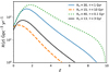	Fig. 3 $ℛ (z)$ ${\cal R}\left( z \right)$ , (Eq. (2)) with different $ℛ_{0}$ ${{\cal R}_0}$ and τ.
In the text

	Fig. 4 Primary BH mass distribution in the default models of BBH-PopA/B; see Eqs. (5) and (7). Here we mark μ, μ + с/γ, and m_реа in the plot in order to provide a rough estimate of these quantities.
In the text

	Fig. 5 M_Z,tot vs. z of SMBBH mergers that occur in the Universe over a timescale of 5 yr for three population models from Klein 16. The data correspond to one realisation.
In the text

	Fig. 6 Distribution density of GW properties of DWD binaries in the simulated catalogue (black contours) as function of GW frequency f_s and GW amplitude A. The blue stars are known DWDs used as VBs.
In the text

	Fig. 7 The averaged histograms of μ, M and D of EMRIs happen in 1 yr, assuming different population models from Babak l7.
In the text

	Fig. 8 Upper panel: noise curves of the default detectors. Lower panel: aLIGO in design vs. customised settings (arm length = 4km, laser power = 125 W).
In the text

Fig. 9

Upper panel: square root of the PSD noise TDI-X corresponding to different LISA configurations. The solid curves are the total PSD, while the dashed curves are the contribution from the confusion GWDs. The bundle of curves in the same colour corresponds to T_obs = 1, 2, 4, and 5 yr from top to bottom; Lower panel: sensitivity curves corresponding to different arm lengths and T_obs. The solid curves are the total curve, while the dashed curves are the contribution from the confusion GWDs. The bundle of curves in the same colour corresponds to T_obs = 1, 2, 4, and 5 yr from top to bottom.

In the text

	Fig. 10 Modulus of frequency domain TDI-X responses to GWs from different SMBBHs (whose parameters are listed in Table 2). The solid curves correspond to LISA with 5 Gm laser arms, and dashed curves correspond to a 2.5 Gm arms configuration.
In the text

	Fig. 11 Frequency domain LISA responses to GW from a DWD: The blue and orange lines correspond to two different LISA configurations; solid and dashed lines correspond to responses calculated with numerical and analytical methods respectively.
In the text

	Fig. 12 Frequency domain TDI-X responses to EMRI AK waveform, which correspond to three EMRI systems and two L designs of LISA.
In the text

	Fig. 13 Noise spectra of the pulsars. Blue curves correspond to known pulsars in existing PTAs, and orange curves are simulated new pulsars.
In the text

	Fig. 14 Galactic distribution of the PTAs. The blue dots indicate the pulsars from current IPTA, and the orange dots indicate the simulated new pulsars. The size of the markers is proportional to the number of TOAs of the corresponding pulsar.
In the text

Fig. 15

Simulated catalogue vs. catalogue from real observations: aLIGO-design-1 year: simulated catalogue from 1 yr of observation by aLIGO with designed noise performance on BBH, marked with blue crosses; aLIGO-O3-1 yr: simulated catalogue from 1 yr of observation by aLIGO with O3 noise performance on BBH, marked with orange dots; GWTC-3 (BBH): BBH events in GWTC-3, marked with green star symbols.

In the text

	Fig. 16 m₁ distribution (upper panel) and the number density as function of redshift (lowerpanel) in the catalogue for 1 month of observation of BBH mergers by ET (solid blue line). The integral of the latter is the total number of detections. As a comparison, we plot the distribution of BBH mergers for the whole Universe within 1 month (dashed orange line).
In the text

	Fig. 17 The same as Fig. 15, but for 10 yr observation of DNS with eLIGO (design and O3 sensitivity).
In the text

	Fig. 18 Total mass distribution (upperpanel) and the number density as functions of redshift (right panel) in the catalogue of 1 yr of observation of DNS mergers by ET (solid blue). The integral of the latter is the total number of detections. The dashed orange curve is the same but for the whole Universe within 1 yr.
In the text

	Fig. 19 As in Fig. 15 but with BHNSs: aLIGO-design-10yr: simulated catalogue from 10 yr of observation by aLIGO with designed noise performance on BHNSs, marked with blue crosses; aLIGO-O3-10 yr: simulated catalogue from 10 yr of observation by aLIGO with O3 noise performance on BHNS, marked with orange dots.
In the text

	Fig. 20 Probability density distribution as a function of m_● (upper panel) and m_n (middle panel), and number density as a function of red-shift (lower panel) for 10 yr of observation of BHNS mergers by ET. The integral of the latter is the total number of detections. The orange lines show the intrinsic distributions.
In the text

	Fig. 21 Redshifted chirp masses and the redshift of the total events (markers) and detected ones (squares on top of markers) by the standard LISA configuration in 5 yr. Orange, blue, and green markers correspond to Q3_nodelay, рорЗ, and Q3_delays population models, respectively. The underlying S/N cutoff is 8.
In the text

Fig. 22

Distributions of relative uncertainties and the uncertainties of the sky location of the events in the simulated catalogue: Upper: distribution of relative uncertainties on the total masses in the catalogue of SMBBH mergers detected by LISA in 5 yr. Solid lines are for default LISA and dashed lines are for 5 Gm arm length. Middle: same as the upper panel, but on the relative uncertainties on the luminosity distances. Lower: same as the upper two panels, but on uncertainties of the sky location (deg²).

In the text

	Fig. 23 Detected number of DWDs with the default LISA and a larger LISA with 5 million km arms as a function of the observation duration. We use a threshold S/N ρ_⋆ = 7.
In the text

	Fig. 24 Pre-calculated S/N by Babak 17 compared to the S/N of this work for the same catalogue, for 1 yr of observation of the Ml population.
In the text

	Fig. 25 Histogram of the SNR of the bright EMRIs in catalogue of BabaklX The blue histogram indicate the SNR calculated in this work, and the orange histogram is that pre-calculated by Babak17 using a slightly different LISA noise and waveform.
In the text

	Fig. 26 Histogram of relative uncertainties on the mass of the lighter component μ, the mass of the heavier component M, and the distance D, and the uncertainties on the sky location dΩ. in a catalogue of EMRIs detected by the default LISA for two years of observation. The S/N cutoff is setto 20.
In the text

	Fig. 27 Sensitivity plot for an individual SMBBH as a function of frequency for ρ_cri = 10 and averaged over the celestial sphere for different PTAs.
In the text

	Fig. A.1 Conversion between different kinds of LISA responses
In the text

Current usage metrics show cumulative count of Article Views (full-text article views including HTML views, PDF and ePub downloads, according to the available data) and Abstracts Views on Vision4Press platform.

Data correspond to usage on the plateform after 2015. The current usage metrics is available 48-96 hours after online publication and is updated daily on week days.

Initial download of the metrics may take a while.

[1] Abbott, B. P., Abbott, R., Abbott, T. D., et al. 2016a, Phys. Rev. Lett., 116, 061102 [Google Scholar]

[2] Abbott, B. P., Abbott, R., Abbott, T. D., et al. 2016b, ApJ, 818, L22 [Google Scholar]

[3] Abbott, B. P., Abbott, R., Abbott, T. D., et al. 2017a, Phys. Rev. Lett., 119, 161101 [Google Scholar]

[4] Abbott, B. P., Abbott, R., Abbott, T. D., et al. 2017b, ApJ, 848, L12 [Google Scholar]

[5] Abbott, B. P., Abbott, R., Abbott, T. D., et al. 2017c, ApJ, 848, L13 [CrossRef] [Google Scholar]

[6] Abbott, B. P., Abbott, R., Abbott, T. D., et al. 2017d, Nature, 551, 85 [Google Scholar]

[7] Abbott, B. P., Abbott, R., Abbott, T. D., et al. 2017e, ApJ, 850, L39 [NASA ADS] [CrossRef] [Google Scholar]

[8] Abbott, B. P., Abbott, R., Abbott, T. D., et al. 2017f, ApJ, 850, L40 [NASA ADS] [CrossRef] [Google Scholar]

[9] Abbott, B. P., Abbott, R., Abbott, T. D., et al. 2018a, Phys. Rev. Lett., 121, 161101 [Google Scholar]

[10] Abbott, B. P., Abbott, R., Abbott, T. D., et al. 2018b, Phys. Rev. Lett., 120, 091101 [CrossRef] [Google Scholar]

[11] Abbott, B. P., Abbott, R., Abbott, T. D., et al. 2019a, Phys. Rev. X, 9, 011001 [Google Scholar]

[12] Abbott, B. P., Abbott, R., Abbott, T. D., et al. 2019b, Phys. Rev. X, 9, 031040 [Google Scholar]

[13] Abbott, B. P., Abbott, R., Abbott, T. D., et al. 2019c, Phys. Rev. Lett., 122, 061104 [NASA ADS] [CrossRef] [Google Scholar]

[14] Abbott, B. P., Abbott, R., Abbott, T. D., et al. 2019d, Phys. Rev. Lett., 123, 011102 [Google Scholar]

[15] Abbott, B. P., Abbott, R., Abbott, T. D., et al. 2019e, ApJ, 882, L24 [Google Scholar]

[16] Abbott, B. P., Abbott, R., Abbott, T. D., et al. 2020a, Class. Quant. Grav., 37, 045006 [NASA ADS] [CrossRef] [Google Scholar]

[17] Abbott, R., Abbott, T. D., Abraham, S., et al. 2020b, Phys. Rev. D, 102, 043015 [NASA ADS] [CrossRef] [Google Scholar]

[18] Abbott, R., Abbott, T. D., Abraham, S., et al. 2020c, Phys. Rev. X 11, 021053 [NASA ADS] [Google Scholar]

[19] Abbott, R., Abbott, T. D., Abraham, S., et al. 2020d, ApJ, 896, L44 [Google Scholar]

[20] Abbott, R., Abbott, T. D., Abraham, S., et al. 2021a, ApJ, 915, L5 [NASA ADS] [CrossRef] [Google Scholar]

[21] Abbott, R., Abbott, T. D., Acernese, F., et al. 2021b, https://dcc.ligo.org/public/0170/P2000318/007/o3b_catalog.pdf [Google Scholar]

[22] Abbott, R., Abbott, T. D., Abraham, S., et al. 2021c, ApJL, 913, L7 [NASA ADS] [CrossRef] [Google Scholar]

[23] Acernese, F., Agathos, M., Agatsuma, K., et al. 2015, Class. Quant. Grav., 32, 024001 [Google Scholar]

[24] Aggarwal, K., Arzoumanian, Z., Baker, P. T., et al. 2019, ApJ, 880, 116 [NASA ADS] [CrossRef] [Google Scholar]

[25] Aggarwal, K., Arzoumanian, Z., Baker, P. T., et al. 2020, ApJ, 889, 38 [NASA ADS] [CrossRef] [Google Scholar]

[26] Aggarwal, N., Aguiar, O. D., Bauswein, A., et al. 2021, Liv. Rev. Relat., 24, 4 [NASA ADS] [CrossRef] [Google Scholar]

[27] Ajith, P., Hannam, M., Husa, S., et al. 2011, Phys. Rev. Lett., 106, 241101 [NASA ADS] [CrossRef] [Google Scholar]

[28] Alam, M. F., Arzoumanian, Z., Baker, P. T., et al. 2021, ApJS, 252, 5 [Google Scholar]

[29] Amaro-Seoane, P., Gair, J. R., Freitag, M., et al. 2007, Class. Quant. Grav., 24, R113 [NASA ADS] [CrossRef] [Google Scholar]

[30] Amaro-Seoane, P., Audley, H., Babak, S., et al. 2017, Arxiv e-prints [arXiv:1702.00786] [Google Scholar]

[31] Anholm, M., Ballmer, S., Creighton, J. D. E., et al. 2009, Phys. Rev. D, 79, 084030 [NASA ADS] [CrossRef] [Google Scholar]

[32] Antoniadis, J., Arzoumanian, Z., Babak, S., et al. 2022, MNRAS, 510, 4873 [NASA ADS] [CrossRef] [Google Scholar]

[33] Armstrong, J. W., Estabrook, F. B., & Tinto, M. 1999, ApJ, 527, 814 [NASA ADS] [CrossRef] [Google Scholar]

[34] Arzoumanian, Z., Baker, P. T., Brazier, A., et al. 2018, ApJ, 859, 47 [NASA ADS] [CrossRef] [Google Scholar]

[35] Arzoumanian, Z., Baker, P. T., Blumer, H., et al. 2020, ApJ, 905, L34 [NASA ADS] [CrossRef] [Google Scholar]

[36] Astropy Collaboration (Robitaille, T. P., et al.) 2013, A&Amp;A, 558, A33 [NASA ADS] [CrossRef] [EDP Sciences] [Google Scholar]

[37] Astropy Collaboration (Price-Whelan, A. M., et al.) 2018, AJ, 156, 123 [Google Scholar]

[38] Babak, S., & Sesana, A. 2012, Phys. Rev. D, 85, 044034 [NASA ADS] [CrossRef] [Google Scholar]

[39] Babak, S., Baker, J. G., Benacquista, M. J., et al. 2010, Class. Quant. Grav., 27, 084009 [NASA ADS] [CrossRef] [Google Scholar]

[40] Babak, S., Petiteau, A., Sesana, A., et al. 2016, MNRAS, 455, 1665 [NASA ADS] [CrossRef] [Google Scholar]

[41] Babak, S., Gair, J., Sesana, A., et al. 2017, Phys. Rev. D, 95, 103012 [NASA ADS] [CrossRef] [Google Scholar]

[42] Barack, L., & Cutler, C. 2004, Phys. Rev. D, 69, 082005 [NASA ADS] [CrossRef] [Google Scholar]

[43] Barausse, E. 2012, MNRAS, 423, 2533 [NASA ADS] [CrossRef] [Google Scholar]

[44] Barausse, E., Berti, E., Hertog, T., et al. 2020, Gen. Relat. Grav., 52, 81 [CrossRef] [Google Scholar]

[45] Barke, S., Wang, Y., Esteban Delgado, J. J., et al. 2015, Class. Quant. Grav., 32, 095004 [NASA ADS] [CrossRef] [Google Scholar]

[46] Belczynski, K., Kalogera, V., & Bulik, T. 2002, ApJ, 572, 407 [NASA ADS] [CrossRef] [Google Scholar]

[47] Belczynski, K., Holz, D. E., Bulik, T., et al. 2016, Nature, 534, 512 [NASA ADS] [CrossRef] [Google Scholar]

[48] Berti, E., Cardoso, V., & Will, C. M. 2006, Phys. Rev. D, 73, 064030 [NASA ADS] [CrossRef] [Google Scholar]

[49] Brown, D. D., Jones, P., Rowlinson, S., et al. 2020, SoftwareX, 12, 100613 [NASA ADS] [CrossRef] [Google Scholar]

[50] Burke-Spolaor, S., Taylor, S. R., Charisi, M., et al. 2019, A&Amp;A Rev., 27, 5 [Google Scholar]

[51] Caprini, C., & Figueroa, D. G. 2018, Class. Quant. Grav., 35, 163001 [NASA ADS] [CrossRef] [Google Scholar]

[52] Chatziioannou, K., Cotesta, R., Ghonge, S., et al. 2019, Phys. Rev. D, 100, 104015 [NASA ADS] [CrossRef] [Google Scholar]

[53] Chruślińska, M., Nelemans, G., & Belczynski, K. 2019, MNRAS, 482, 5012 [CrossRef] [Google Scholar]

[54] Chruślińska, M., Jeřábková, T., Nelemans, G., et al. 2020, A&A, 636, A10 [NASA ADS] [CrossRef] [EDP Sciences] [Google Scholar]

[55] Chua, A. J. K., & Gair, J. R. 2015, Class. Quant. Grav., 32, 232002 [NASA ADS] [CrossRef] [Google Scholar]

[56] Chua, A. J. K., Moore, C. J., & Gair, J. R. 2017, Phys. Rev. D, 96, 044005 [NASA ADS] [CrossRef] [Google Scholar]

[57] Clark, J. P. A., van den Heuvel, E. P. J., & Sutantyo, W. 1979, A&A, 72, 120 [NASA ADS] [Google Scholar]

[58] Colpi, M. 2014, Space Sci. Rev., 183, 189 [Google Scholar]

[59] Cornish, N. J., & Littenberg, T. B. 2007, Phys. Rev. D, 76, 083006 [NASA ADS] [CrossRef] [Google Scholar]

[60] Coulter, D. A., Foley, R. J., Kilpatrick, C. D., et al. 2017, Science, 358, 1556 [NASA ADS] [CrossRef] [Google Scholar]

[61] Dahal, P. K. 2020, J. Astrophys. Astron., 41, 8 [NASA ADS] [CrossRef] [Google Scholar]

[62] Damour, T., & Vilenkin, A. 2001, Phys. Rev. D, 64, 064008 [NASA ADS] [CrossRef] [Google Scholar]

[63] Damour, T., & Vilenkin, A. 2005, Phys. Rev. D, 71, 063510 [NASA ADS] [CrossRef] [Google Scholar]

[64] Demorest, P. B., Ferdman, R. D., Gonzalez, M. E., et al. 2013, ApJ, 762, 94 [Google Scholar]

[65] Desvignes, G., Caballero, R. N., Lentati, L., et al. 2016, MNRAS, 458, 3341 [Google Scholar]

[66] Detweiler, S. 1979, ApJ, 234, 1100 [NASA ADS] [CrossRef] [Google Scholar]

[67] de Mink, S. E., & Belczynski, K. 2015, ApJ, 814, 58 [Google Scholar]

[68] Divyajyoti, Baxi, P., Mishra, C. K., et al. 2021, Phys. Rev. D, 104, 084080 [NASA ADS] [CrossRef] [Google Scholar]

[69] Dominik, M., Berti, E., O’Shaughnessy, R., et al. 2015, ApJ, 806, 263 [Google Scholar]

[70] Ellis, J. A. 2013, Class. Quant. Grav., 30, 224004 [NASA ADS] [CrossRef] [Google Scholar]

[71] Ellis, J. A., Siemens, X., & Creighton, J. D. E. 2012, ApJ, 756, 175 [NASA ADS] [CrossRef] [Google Scholar]

[72] Estabrook, F. B., Tinto, M., & Armstrong, J. W. 2000, Phys. Rev. D, 62, 042002 [NASA ADS] [CrossRef] [Google Scholar]

[73] Farr, W. M., Sravan, N., Cantrell, A., et al. 2011, ApJ, 741, 103 [NASA ADS] [CrossRef] [Google Scholar]

[74] Farrow, N., Zhu, X.-J., & Thrane, E. 2019, ApJ, 876, 18 [NASA ADS] [CrossRef] [Google Scholar]

[75] Ferrarese, L., & Merritt, D. 2000, ApJ, 539, L9 [Google Scholar]

[76] Fryer, C. L., & Kalogera, V. 2001, ApJ, 554, 548 [Google Scholar]

[77] Gair, J. R., Barack, L., Creighton, T., et al. 2004, Class. Quant. Grav., 21, S1595 [NASA ADS] [CrossRef] [Google Scholar]

[78] Goetz, E., & Riles, K. 2011, Class. Quant. Grav., 28, 215006 [NASA ADS] [CrossRef] [Google Scholar]

[79] González, G., Viceré, A., & Wen, L. 2013, Front. Phys., 8, 771 [CrossRef] [Google Scholar]

[80] Grishchuk, L. P. 1976, Sov. J. Exp. Theor. Phys. Lett., 23, 293 [NASA ADS] [Google Scholar]

[81] Grishchuk, L. P. 1977, Eighth Texas Symposium on Relativistic Astrophysics, 302, 439 [NASA ADS] [Google Scholar]

[82] Harry, G. M., & LIGO Scientific Collaboration 2010, Class. Quant. Grav., 27, 084006 [NASA ADS] [CrossRef] [Google Scholar]

[83] Hellings, R. W., & Downs, G. S. 1983, ApJ, 265, L39 [NASA ADS] [CrossRef] [Google Scholar]

[84] Hild, S., Chelkowski, S., & Freise, A. 2008, ArXiv e-prints [arXiv:0810.0604] [Google Scholar]

[85] Hild, S., Chelkowski, S., Freise, A., et al. 2010, Class. Quant. Grav., 27, 015003 [NASA ADS] [CrossRef] [Google Scholar]

[86] Hild, S., Abernathy, M., Acernese, F., et al. 2011, Class. Quant. Grav., 28, 094013 [Google Scholar]

[87] Hobbs, G. 2013, Class. Quant. Grav., 30, 224007 [NASA ADS] [CrossRef] [Google Scholar]

[88] Hobbs, G., & Dai, S. 2017, Natl. Sci. Rev., 4, 707 [CrossRef] [Google Scholar]

[89] Hobbs, G. B., Edwards, R. T., & Manchester, R. N. 2006, MNRAS, 369, 655 [Google Scholar]

[90] Hobbs, G., Archibald, A., Arzoumanian, Z., et al. 2010a, Class. Quant. Grav., 27, 084013 [NASA ADS] [CrossRef] [Google Scholar]

[91] Hobbs, G., Lyne, A. G., & Kramer, M. 2010b, MNRAS, 402, 1027 [NASA ADS] [CrossRef] [Google Scholar]

[92] Huang, S.-J., Hu, Y.-M., Korol, V., et al. 2020, Phys. Rev. D, 102, 063021 [NASA ADS] [CrossRef] [Google Scholar]

[93] Hughes, S. A., Warburton, N., Khanna, G., et al. 2021, Phys. Rev. D, 103, 104014 [NASA ADS] [CrossRef] [Google Scholar]

[94] Inayoshi, K., Visbal, E., & Haiman, Z. 2020, ARA&A, 58, 27 [NASA ADS] [CrossRef] [Google Scholar]

[95] Janssen, G., Hobbs, G., McLaughlin, M., et al. 2015, Advancing Astrophysics with the Square Kilometre Array (AASKA14), 37 [Google Scholar]

[96] Jenet, F. A., Lommen, A., Larson, S. L., et al. 2004, ApJ, 606, 799 [NASA ADS] [CrossRef] [Google Scholar]

[97] Jenet, F. A., Hobbs, G. B., Lee, K. J., et al. 2005, ApJ, 625, L123 [NASA ADS] [CrossRef] [Google Scholar]

[98] Kagra Collaboration (Akutsu, T., et al.) 2019, Nat. Astron., 3, 35 [NASA ADS] [CrossRef] [Google Scholar]

[99] Kawamura, S., Nakamura, T., Ando, M., et al. 2006, Class. Quant. Grav., 23, S125 [NASA ADS] [CrossRef] [Google Scholar]

[100] Kiziltan, B., Kottas, A., De Yoreo, M., et al. 2013, ApJ, 778, 66 [NASA ADS] [CrossRef] [Google Scholar]

[101] Klein, A., Barausse, E., Sesana, A., et al. 2016, Phys. Rev. D, 93, 024003 [NASA ADS] [CrossRef] [Google Scholar]

[102] Kormendy, J., & Ho, L. C. 2013, ARA&A, 51, 511 [Google Scholar]

[103] Korol, V., Rossi, E. M., Groot, P. J., et al. 2017, MNRAS, 470, 1894 [NASA ADS] [CrossRef] [Google Scholar]

[104] Kovetz, E. D., Cholis, I., Breysse, P. C., et al. 2017, Phys. Rev. D, 95, 103010 [NASA ADS] [CrossRef] [Google Scholar]

[105] Kramer, M., & Champion, D. J. 2013, Class. Quant. Grav., 30, 224009 [NASA ADS] [CrossRef] [Google Scholar]

[106] Kupfer, T., Korol, V., Shah, S., et al. 2018, MNRAS, 480, 302 [NASA ADS] [CrossRef] [Google Scholar]

[107] Lamberts, A., Garrison-Kimmel, S., Hopkins, P. F., et al. 2018, MNRAS, 480, 2704 [NASA ADS] [CrossRef] [Google Scholar]

[108] Lamberts, A., Blunt, S., Littenberg, T. B., et al. 2019, MNRAS, 490, 5888 [NASA ADS] [CrossRef] [Google Scholar]

[109] Lasky, P. D., Mingarelli, C. M. F., Smith, T. L., et al. 2016, Phys. Rev. X, 6, 011035 [NASA ADS] [Google Scholar]

[110] Lau, M. Y. M., Mandel, I., Vigna-Gómez, A., et al. 2020, MNRAS, 492, 3061 [NASA ADS] [CrossRef] [Google Scholar]

[111] Lentati, L., Taylor, S. R., Mingarelli, C. M. F., et al. 2015, MNRAS, 453, 2576 [Google Scholar]

[112] LIGO Scientific Collaboration (Aasi, J., et al.) 2015, Class. Quant. Grav., 32, 074001 [Google Scholar]

[113] Linde, A. D. 1982, Phys. Lett. B, 108, 389 [Google Scholar]

[114] Lipunov, V. M., Postnov, K. A., & Prokhorov, M. E. 1997, New A, 2, 43 [NASA ADS] [CrossRef] [Google Scholar]

[115] London, L., Khan, S., Fauchon-Jones, E., et al. 2018, Phys. Rev. Lett., 120, 161102 [NASA ADS] [CrossRef] [Google Scholar]

[116] Luo, J., Chen, L.-S., Duan, H.-Z., et al. 2016, Class. Quant. Grav., 33, 035010 [NASA ADS] [CrossRef] [Google Scholar]

[117] Madau, P., & Dickinson, M. 2014, ARA&A, 52, 415 [Google Scholar]

[118] Maggiore, M. 2008, Gravitational Waves: Volume 1: Theory and Experiments (Oxford University Press) [Google Scholar]

[119] Maggiore, M., Van Den Broeck, C., Bartolo, N., et al. 2020, J. Cosmology Astropart. Phys., 2020, 050 [CrossRef] [Google Scholar]

[120] Magorrian, J., Tremaine, S., Richstone, D., et al. 1998, AJ, 115, 2285 [Google Scholar]

[121] Mapelli, M., Giacobbo, N., Ripamonti, E., et al. 2017, MNRAS, 472, 2422 [NASA ADS] [CrossRef] [Google Scholar]

[122] McLaughlin, M. A. 2013, Class. Quant. Grav., 30, 224008 [NASA ADS] [CrossRef] [Google Scholar]

[123] McWilliams, S. T., Ostriker, J. P., & Pretorius, F. 2014, ApJ, 789, 156 [NASA ADS] [CrossRef] [Google Scholar]

[124] McWilliams, S. T., Caldwell, R., Holley-Bockelmann, K., et al. 2019, ArXiv eprints [arXiv:1903.04592] [Google Scholar]

[125] Mehta, A. K., Mishra, C. K., Varma, V., et al. 2017, Phys. Rev. D, 96, 124010 [NASA ADS] [CrossRef] [Google Scholar]

[126] Mei, J., Bai, Y.-Z., Bao, J., et al. 2021, Progr. Theor. Exp. Phys., 2021, 05A107 [CrossRef] [Google Scholar]

[127] Miller, M. C., & Miller, J. M. 2015, Phys. Rep., 548, 1 [NASA ADS] [CrossRef] [Google Scholar]

[128] Mills, C., & Fairhurst, S. 2021, Phys. Rev. D, 103, 024042 [NASA ADS] [CrossRef] [Google Scholar]

[129] Moe, M., & Di Stefano, R. 2017, ApJS, 230, 15 [Google Scholar]

[130] Murray, I., Adams, R. P., MacKay, D. J. C. 2010, Proceedings of the Thirteenth International Conference on Artificial Intelligence and Statistics, 541 [Google Scholar]

[131] Neal, R.M. 1999, Bayesian Stat., 6, 475 [Google Scholar]

[132] Nelemans, G. 2018, ArXiv e-prints [arXiv:1807.01060] [Google Scholar]

[133] Nelemans, G., Yungelson, L. R., & Portegies Zwart, S. F. 2001, A&A, 375, 890 [NASA ADS] [CrossRef] [EDP Sciences] [Google Scholar]

[134] Nissanke, S., Vallisneri, M., Nelemans, G., et al. 2012, ApJ, 758, 131 [NASA ADS] [CrossRef] [Google Scholar]

[135] Ölmez, S., Mandic, V., & Siemens, X. 2010, Phys. Rev. D, 81, 104028 [CrossRef] [Google Scholar]

[136] Ott, C. D. 2009, Class. Quant. Grav., 26, 204015 [NASA ADS] [CrossRef] [Google Scholar]

[137] Özel, F., Psaltis, D., Narayan, R., et al. 2012, ApJ, 757, 55 [CrossRef] [Google Scholar]

[138] Petiteau, A., Babak, S., Sesana, A., et al. 2013, Phys. Rev. D, 87, 064036 [NASA ADS] [CrossRef] [Google Scholar]

[139] Phinney, E. S. 1991, ApJ, 380, L17 [NASA ADS] [CrossRef] [Google Scholar]

[140] Phinney, E. S. 2001, ArXiv e-prints [arXiv:astro-ph/0108028] [Google Scholar]

[141] Pian, E., D’Avanzo, P., Benetti, S., et al. 2017, Nature, 551, 67 [Google Scholar]

[142] Planck Collaboration I. 2016, A&A, 594, A1 [NASA ADS] [CrossRef] [EDP Sciences] [Google Scholar]

[143] Porayko, N. K., Noutsos, A., Tiburzi, C., et al. 2019, MNRAS, 483, 4100 [Google Scholar]

[144] Portegies Zwart, S. F., & McMillan, S. L. W. 2000, ApJ, 528, L17 [Google Scholar]

[145] Postnov, K. A., & Kuranov, A. G. 2019, MNRAS, 483, 3288 [NASA ADS] [CrossRef] [Google Scholar]

[146] Postnov, K. A., & Yungelson, L. R. 2014, Liv. Rev. Relat., 17, 3 [NASA ADS] [CrossRef] [Google Scholar]

[147] Punturo, M., Abernathy, M., Acernese, F., et al. 2010, Class. Quant. Grav., 27, 194002 [Google Scholar]

[148] Regimbau, T., Dent, T., Del Pozzo, W., et al. 2012, Phys. Rev. D, 86, 122001 [NASA ADS] [CrossRef] [Google Scholar]

[149] Reitze, D., Adhikari, R. X., Ballmer, S., et al. 2019, BAAS, 51, 035 [NASA ADS] [Google Scholar]

[150] Robson, T., Cornish, N. J., & Liu, C. 2019, Class. Quant. Grav., 36, 105011 [NASA ADS] [CrossRef] [Google Scholar]

[151] Rodriguez, C. L., Farr, B., Farr, W. M., et al. 2013, Phys. Rev. D, 88, 084013 [NASA ADS] [CrossRef] [Google Scholar]

[152] Ruiter, A. J., Belczynski, K., Benacquista, M., et al. 2010, ApJ, 717, 1006 [NASA ADS] [CrossRef] [Google Scholar]

[153] Sathyaprakash, B. S., & Schutz, B. F. 2009, Liv. Rev. Relat., 12, 2 [NASA ADS] [CrossRef] [Google Scholar]

[154] Sazhin, M. V. 1978, Soviet Ast., 22, 36 [NASA ADS] [Google Scholar]

[155] Sesana, A. 2016, Phys. Rev. Lett., 116, 231102 [NASA ADS] [CrossRef] [Google Scholar]

[156] Sesana, A., & Vecchio, A. 2010, Phys. Rev. D, 81, 104008 [NASA ADS] [CrossRef] [Google Scholar]

[157] Sesana, A., Haardt, F., Madau, P., et al. 2005, ApJ, 623, 23 [NASA ADS] [CrossRef] [Google Scholar]

[158] Sesana, A., Vecchio, A., & Colacino, C. N. 2008, MNRAS, 390, 192 [NASA ADS] [CrossRef] [Google Scholar]

[159] Sesana, A., Lamberts, A., & Petiteau, A. 2020, MNRAS, 494, L75 [Google Scholar]

[160] Schneider, R., Ferrari, V., Matarrese, S., et al. 2001, MNRAS, 324, 797 [NASA ADS] [CrossRef] [Google Scholar]

[161] Schutz, B. F. 1989, Class. Quant. Grav., 6, 1761 [NASA ADS] [CrossRef] [Google Scholar]

[162] Schutz, K., & Ma, C.-P. 2016, MNRAS, 459, 1737 [NASA ADS] [CrossRef] [Google Scholar]

[163] Shannon, R. M., Ravi, V., Coles, W. A., et al. 2013, Science, 342, 334 [NASA ADS] [CrossRef] [Google Scholar]

[164] Shannon, R. M., Ravi, V., Lentati, L. T., et al. 2015, Science, 349, 1522 [NASA ADS] [CrossRef] [Google Scholar]

[165] Siemens, X., Creighton, J., Maor, I., et al. 2006, Phys. Rev. D, 73, 105001 [NASA ADS] [CrossRef] [Google Scholar]

[166] Siemens, X., Mandic, V., & Creighton, J. 2007, Phys. Rev. Lett., 98, 111101 [NASA ADS] [CrossRef] [Google Scholar]

[167] Starobinsky, A. A. 1980, Phys. Lett. B, 91, 99 [Google Scholar]

[168] Talbot, C., & Thrane, E. 2018, ApJ, 856, 173 [NASA ADS] [CrossRef] [Google Scholar]

[169] Tauris, T. M. 2018, Phys. Rev. Lett., 121, 131105 [NASA ADS] [CrossRef] [Google Scholar]

[170] Timpano, S. E., Rubbo, L. J., & Cornish, N. J. 2006, Phys. Rev. D, 73, 122001 [NASA ADS] [CrossRef] [Google Scholar]

[171] Thorne, K. S. 1980, Rev. Mod. Phys., 52, 299 [NASA ADS] [CrossRef] [Google Scholar]

[172] Thorne, K. S. 1987, Three Hundred Years of Gravitation, 330 [Google Scholar]

[173] Tinto, M., & Armstrong, J. W. 1999, Phys. Rev. D, 59, 102003 [NASA ADS] [CrossRef] [Google Scholar]

[174] Toonen, S., Nelemans, G., & Portegies Zwart, S. 2012, A&A, 546, A70 [NASA ADS] [CrossRef] [EDP Sciences] [Google Scholar]

[175] van Haasteren, R., Levin, Y., McDonald, P., et al. 2009, MNRAS, 395, 1005 [NASA ADS] [CrossRef] [Google Scholar]

[176] van Haasteren, R., Levin, Y., Janssen, G. H., et al. 2011, MNRAS, 414, 3117 [NASA ADS] [CrossRef] [Google Scholar]

[177] Valentim, R., Rangel, E., & Horvath, J. E. 2011, MNRAS, 414, 1427 [NASA ADS] [CrossRef] [Google Scholar]

[178] Vallisneri, M. 2008, Phys. Rev. D, 77, 042001 [NASA ADS] [CrossRef] [Google Scholar]

[179] Veitch, J., Raymond, V., Farr, B., et al. 2015, Phys. Rev. D, 91, 042003 [NASA ADS] [CrossRef] [Google Scholar]

[180] Verbiest, J. P. W., Lentati, L., Hobbs, G., et al. 2016, MNRAS, 458, 1267 [Google Scholar]

[181] Vitale, S., & Evans, M. 2017, Phys. Rev. D, 95, 064052 [NASA ADS] [CrossRef] [Google Scholar]

[182] Vitale, S., Farr, W. M., Ng, K. K. Y., et al. 2019, ApJ, 886, L1 [NASA ADS] [CrossRef] [Google Scholar]

[183] Yardley, D. R. B., Hobbs, G. B., Jenet, F. A., et al. 2010, MNRAS, 407, 669 [NASA ADS] [CrossRef] [Google Scholar]