© The Authors 2023

1. Introduction

The discovery (LIGO Scientific & Virgo Collaborations 2016) of gravitational waves (GWs) by the LIGO and Virgo experiments, in the 𝒪(100) Hz range of frequencies generated by mergers of black holes (BHs) with masses of 𝒪(10 − 100) M_⊙ (LIGO Scientific, Virgo & KAGRA Collaborations 2021), has opened a new window onto both astrophysics and cosmology. Supermassive black holes (SMBHs) with masses of 𝒪(10⁶ − 10¹⁰) M_⊙ are known to be present in galactic nuclei, and the immediate surroundings of two of them have recently been imaged by the Event Horizon Telescope (Event Horizon Telescope Collaboration 2019, 2022). However, information on intermediate-mass black holes (IMBHs) with masses in the range 𝒪(10³ − 10⁵) M_⊙ (Greene et al. 2020) is less complete. Observations of IMBHs and their mergers would cast light on the uncharted mechanisms that must be presented for SMBHs to form.

A prerequisite for BH mergers is the formation of tightly bound binaries that can radiate GWs efficiently. While there are several well-understood paths for forming compact stellar-mass BHs binaries (e.g., common envelope evolution or dynamical capture in dense stellar environments), the final stage of SMBH binary formation in galaxy mergers is still not fully understood and is commonly known as “the final parsec problem” (Begelman et al. 1980). However, observations of quasar optical variability provide indirect evidence for the existence of some tight binary SMBHs in the regime where the emission of GWs must already have a noticeable effects on their orbital evolution (Rieger & Mannheim 2000; De Paolis et al. 2002, 2004; Valtonen 2008; Boroson & Lauer 2009; Iguchi et al. 2010; Graham et al. 2015; O’Neill et al. 2022; Kovačević et al. 2022)¹. The GW data will be essential for a better understanding how SMBHs overcome the “final parsec” obstacle, and how the assembly of the SMBH population proceeds in general.

Pulsar timing arrays (PTAs) are potentially sensitive to GWs in the nHz range, while NANOGrav and other PTAs have recently reported evidence for a common-spectrum stochastic process (Arzoumanian et al. 2020; Goncharov et al. 2021; Chen et al. 2021; Antoniadis et al. 2022). Their signals have power spectra that are consistent with predictions based on inspiralling binary SMBH models (Phinney 2001)², but they have not (yet) detected the Hellings-Downs quadrupolar signature that is characteristic of GWs (Hellings & Downs 1983)³.

The BH merger interpretation of the PTA measurements does not provide direct information on the masses of the infalling BHs, which requires the modelling and measurements of this stochastic GW background in different frequency ranges (Sesana et al. 2008). The purpose of this paper is to illustrate how future measurements of the GW spectrum due to unresolved infall sources and individual binary mergers at frequencies between the PTAs and LIGO/Virgo will be able to extend the PTA measurements to lower black-hole mass ranges, probing models for the assembly of SMBHs, and perhaps obtaining direct evidence for the mergers of IMBHs. We take as the amplitude of the common-spectrum process measured by the PTAs $A=2.8_{-0.8}^{+1.2}\times {10}^{-15}$ at a reference frequency of 1/yr, as found by the International Pulsar Timing Array (IPTA; Antoniadis et al. 2022) assuming the spectral index of α = −2/3 expected from inspiralling SMBHs, which is consistent with other measurements.

We use examples of next-generation GW detectors the planned LISA laser interferometer (Berti et al. 2006), whose peak sensitivity is at frequencies 𝒪(10⁻⁴ − 10⁻²) Hz, the proposed ET laser interferometer (Sathyaprakash et al. 2012), whose peak sensitivity is at frequencies 𝒪(1 − 10²) Hz and the projected AION-km and AEDGE atom interferometers (Badurina et al. 2020; El-Neaj et al. 2020), whose peak sensitivities would be in the range of 𝒪(10⁻² − 1) Hz. We show that, while none of these detectors would observe a signal from the binary black holes weighing > 𝒪(10⁹) M_⊙ that would probably be responsible for most of the PTA signal, LISA would observe a merger signal from binary black holes weighing 𝒪(10³ − 10⁹) M_⊙ that might contribute part of the PTA signal, while AEDGE would observe a merger signal if there is a population of binary black holes weighing 𝒪(10³ − 10⁶) M_⊙ with a formation history similar to the heavier BHs responsible for the PTA signal.

Throughout this paper, we use natural units with c = 1, G_N = 1.

2. BH merger rate

As a first step towards estimating the BH merger rate, we use the Extended Press-Schechter (EPS) formalism (Press & Schechter 1974; Bond et al. 1991) to calculate the galactic halo mass function,

$$\begin{array}{c}\hfill \frac{\mathrm{d}n(M,t)}{\mathrm{d}lnM}=\frac{{\rho }_0}{M}\sqrt{\frac{2}{\pi }}\frac{\mathrm{d}ln\sigma }{\mathrm{d}lnM}\frac{{\delta }_c(z)}{\sigma (M)}{e}^{-\frac{{\delta }_c{(z)}^2}{2{\sigma }^2(M)}},\end{array}$$(1)

where ρ₀ is the background matter density today, σ²(M) is the variance of the matter fluctuations and δ_c(z) is the critical overdensity for collapse. The latter is given by δ_c(z)≈1.686/D(z) where D(z) is the linear growth function (Dodelson 2003). We calculate σ²(M) from the cold dark matter power spectrum with the Planck 2018 cosmological parameters (Planck Collaboration VI 2020) and the transfer function derived in Eisenstein & Hu (1998). The EPS formalism also gives an estimate for the probability per unit time for a halo of mass M₁ to merge with another one of mass, M₂, at some redshift, z, and become a halo of mass M_f = M₁ + M₂ (Lacey & Cole 1993):

$$\begin{array}{cc}\hfill \frac{\mathrm{d}p(M_1,M_2,t)}{\mathrm{d}t\mathrm{d}{M}_2}& =\frac{1}{M_f}\sqrt{\frac{2}{\pi }}\left|\frac{{\dot{\delta }}_c}{{\delta }_c}\right|\frac{\mathrm{d}ln\sigma }{\mathrm{d}ln{M}_f}{[1-\frac{{\sigma }^2(M_f)}{{\sigma }^2(M_1)}]}^{-\frac{3}{2}}\hfill \\ \hfill & \times \frac{{\delta }_c}{\sigma (M_f)}exp[-\frac{{\delta }_c^2}{2}(\frac{1}{{\sigma }^2(M_f)}-\frac{1}{{\sigma }^2(M_1)})].\hfill \end{array}$$(2)

Defining the halo merger rate kernel:

$$\begin{array}{c}\hfill Q(M_1,M_2,t)\equiv \frac{\mathrm{d}p(M_1,M_2,t)}{\mathrm{d}t\mathrm{d}{M}_2}{\left[\frac{\mathrm{d}n(M_2,t)}{\mathrm{d}{M}_2}\right]}^{-1},\end{array}$$(3)

the halo merger rate is

$$\begin{array}{c}\hfill \frac{\mathrm{d}{R}_h}{\mathrm{d}{M}_1\mathrm{d}{M}_2}=\frac{\mathrm{d}n(M_1,t)}{\mathrm{d}{M}_1}\frac{\mathrm{d}n(M_2,t)}{\mathrm{d}{M}_2}Q(M_1,M_2,t).\end{array}$$(4)

As discussed by Benson et al. (2005), the merger rate kernel Q(M₁, M₂, t) in the EPS formalism is not symmetric in the exchange of M₁ and M₂. However, it was shown by Erickcek et al. (2006) that taking M₁ < M₂ in the merger kernel aptly approximates the result of the Benson-Kamionkowski-Hassani (BKH) merger theory (Benson et al. 2005) where the merger rate kernel is computed from the Smoluchowski coagulation equation and preserves the EPS halo mass function. We will, therefore, require that the first argument of Q is smaller than the second.

In order to estimate the merger rate of central BHs, we must estimate the probability p_occ(m|M, z) that a BH of mass m occupies a halo of mass M, as well as the probability p_merg(m₁, m₂) that the galactic merger leads to a merger of their central BHs. The resulting BH merger rate can be expressed as

$$\begin{array}{cc}& \frac{\mathrm{d}{R}_{\mathrm{BH}}}{\mathrm{d}{m}_1\mathrm{d}{m}_2}={\displaystyle \int }\mathrm{d}{M}_1\mathrm{d}{M}_2{p}_{\mathrm{merg}}(m_1,m_2)\hfill \\ \hfill & \times p_{\mathrm{occ}}(m_1|M_1,z)p_{\mathrm{occ}}(m_2|M_2,z)\frac{\mathrm{d}{R}_h}{\mathrm{d}{M}_1\mathrm{d}{M}_2}.\hfill \end{array}$$(5)

We assume the following simple redshift-dependent relation between the halo mass and the BH mass (Barkana & Loeb 2001; Wyithe & Loeb 2003):

$$\begin{array}{c}\hfill \frac{M_v}{{10}^{12}{M}_{\odot }}=10.5{\left[\frac{{\mathrm{\Omega }}_M(0)}{{\mathrm{\Omega }}_M(z)}\frac{{\mathrm{\Delta }}_c(z)}{18{\pi }^2}\right]}^{-\frac{1}{2}}{(1+z)}^{-\frac{3}{2}}{\left[\frac{m_{\mathrm{BH}}}{{10}^8{M}_{\odot }}\right]}^{\frac{3}{5}},\end{array}$$(6)

where Δ_c(z) = 18π² + 82[Ω_M(z)−1] − 39[Ω_M(z)−1]² is the critical overdensity at virialization, which corresponds to p_occ(m|M) = p_occ(m)δ(m − m_BH(M)). It is generally expected that SMBHs inhabit most large galaxies, and X-ray observations (Miller et al. 2015) constrain the SMBH occupation fraction p_occ(m) to be > 20% for early galaxies with lower stellar masses 10⁷ < M_*/M_⊙ < 10¹⁰. It has been estimated that an initially small occupation fraction may grow at low redshifts (see, e.g., Lippai et al. 2009), which we neglect in this analysis. As we show later, the PTA GW signal is dominated by events in a range 1 ≲ z ≲ 3. The estimated z dependence of p_occ would shift this range towards lower redshifts when compared to a constant p_occ, increasing the observability of BH mergers.

In view of the paucity of information about the merger probability p_merg(m₁, m₂), we model p_merg by a constant for the sake of simplicity. After the galactic merger, various dynamical mechanisms must decrease the size of the SMBH binary below sub-parsec scales in order for a GW emission-driven merger to take place (Begelman et al. 1980). The crossing of the final parsec is determined mostly by binary hardening via stellar loss-cone scattering (Merritt 2013), which can currently be considered the largest source of uncertainty in p_merg. The numerical study of Kelley et al. (2017a), based on a population of 10⁶ − 10¹⁰ M_⊙ BH binaries in the Illustris simulation (Vogelsberger et al. 2014), found for a wide range of model parameters that the coalescing fraction is nearly independent of the total mass of the binary but decreases with the mass ratio. Neglecting the latter dependence should not significantly affect our results, since extreme mass ratio inspirals contribute subdominantly to the GW background. With these assumptions, we obtain:

$$\begin{array}{c}\hfill \frac{\mathrm{d}{R}_{\mathrm{BH}}}{\mathrm{d}{m}_1\mathrm{d}{m}_2}\approx p_{\mathrm{BH}}\frac{\mathrm{d}{M}_1}{\mathrm{d}{m}_1}\frac{\mathrm{d}{M}_2}{\mathrm{d}{m}_2}\frac{\mathrm{d}{R}_h}{\mathrm{d}{M}_1\mathrm{d}{M}_2},\end{array}$$(7)

where p_BH ≡ p_occ(m₁)p_occ(m₂)p_merg denotes the probability that the halo merger leads to a merger of the central SMBHs.

We show in Fig. 1 the BH merger rates as functions of the redshift z, calculated using this approach in three ranges of the total merging BH mass M and normalized relative to the merger probability p_BH discussed above. We see that mergers with total masses M > 10⁹ M_⊙ occur typically at z = 𝒪(1), those with total masses M ∈ (10⁶, 10⁹) M_⊙ occur typically at z = 𝒪(3), and those with total masses M ∈ (10³, 10⁶) M_⊙ occur typically at z = 𝒪(5).

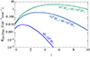Fig. 1. BH merger rates calculated as functions of the redshift z in three ranges of the total merging BH mass M and normalized relative to the merger probability pBH discussed in the text.

In this paper, we use the IPTA measurement (Antoniadis et al. 2022) to normalize p_BH for large BH masses, which circumvents the astrophysical uncertainties related to p_occ and p_merg, and extrapolate it to smaller BH masses. We also comment on the potential mass dependence of p_BH, which is relevant for the GW phenomenology when we extrapolate from the frequency band relevant for PTAs to those to be explored by next-generation GW detectors.

3. Analysis

3.1. The GW energy spectrum

The mean GW energy density spectrum from the SMBH binary population can be estimated as (Phinney 2001):

$$\begin{array}{c}\hfill {\mathrm{\Omega }}_{\mathrm{GW}}(f)\equiv \frac{1}{{\rho }_{\mathrm{c}}}\frac{\mathrm{d}{\rho }_{\mathrm{GW}}}{\mathrm{d}lnf}={\displaystyle \int }\text{d}\lambda \frac{2\pi }{5}\frac{f^3{|\stackrel{\sim }{h}(f)|}^2}{{\rho }_c},\end{array}$$(8)

where $|\stackrel{\sim }{h}(f)|$ denotes the optimal amplitude of the Fourier transform of the GW strain, ${\rho }_{\text{c}}=3H_0^2/8\pi$,

$$\begin{array}{c}\hfill \mathrm{d}\lambda =\mathrm{d}{m}_1\mathrm{d}{m}_2\frac{\mathrm{d}z}{1+z}\frac{\mathrm{d}{V}_c}{\mathrm{d}z}\frac{\mathrm{d}{R}_{\mathrm{BH}}(t)}{\mathrm{d}{m}_1\mathrm{d}{m}_2},\end{array}$$(9)

is the differential merger rate and V_c denotes the comoving volume available at redshift z. We compute $|\stackrel{\sim }{h}(f)|$ using the inspiral-merger-ringdown template (Ajith et al. 2008):

$$\begin{array}{cc}& |\stackrel{\sim }{h}(f)|=\sqrt{\frac{5}{24}}\frac{{\mathcal{M}}_z^{\frac{5}{6}}}{{\pi }^{\frac{2}{3}}{D}_L}\hfill \\ \hfill & \times \{\begin{array}{cc}{f}^{-\frac{7}{6}}\hfill & f<f_{\mathrm{merg}}\hfill \\ f_{\mathrm{merg}}^{-\frac{1}{2}}{f}^{-\frac{2}{3}}\hfill & f_{\mathrm{merg}}\le f<f_{\mathrm{ring}}\hfill \\ f_{\mathrm{merg}}^{-\frac{1}{2}}{f}_{\mathrm{ring}}^{-\frac{2}{3}}\frac{{\sigma }^2}{4{(f-f_{\mathrm{ring}})}^2+{\sigma }^2}\hfill & f_{\mathrm{ring}}\le f<f_{\mathrm{cut}},\hfill \end{array}\hfill \end{array}$$(10)

where the redshift-dependent chirp mass, ℳ_z, is given in terms of the total mass, M, and the symmetric mass ratio η ≡ m₁m₂/M² of the binary by ${\mathcal{M}}_z\equiv (1+z){\mathcal{M}}_0=(1+z)M{\eta }^{\frac{3}{5}}$, and D_L denotes the luminosity distance of the binary. This implies the canonical ${\mathrm{\Omega }}_{\mathrm{GW}}\propto f^{\frac{2}{3}}$ scaling during the inspiral phase (Phinney 2001). The frequencies f_merg, f_ring, f_cut, and σ are parameterised as $f_j={\eta }^{\frac{5}{3}}(a_j{\eta }^2+b_j\eta +c_j)/(\pi {\mathcal{M}}_z)$ where a_j, b_j, and c_j are coefficients whose fitted values are given in Table I of Ajith et al. (2008).

We comment briefly on potential uncertainties in the GW energy density spectrum. If orbital decay is driven by other processes in addition to GW emission, such as viscous drag, then the coalescence time is shortened and the total GW spectrum is suppressed by a factor of T_tot/T_GW, where T_tot, T_GW denote the characteristic hardening timescales (Kocsis & Sesana 2011; Kelley et al. 2017a). Here we omit this effect, assuming that the signal is dominated by binaries for which the hardening is driven mainly by GW emission. Additionally, we consider only circular binaries, which, in the inspiral phase, radiate monochromatically at twice the orbital frequency. We note, however, that the GW spectrum of eccentric binaries would contain higher harmonics, with the fundamental harmonic (at the orbital frequency) becoming dominant at eccentricities e > 0.4 (Taylor et al. 2016). In addition, the GW luminosity would be enhanced by a factor of $(1+73/24e^2+37/96e^4)/{(1-e^2)}^{\frac{7}{2}}$ (Peters & Mathews 1963; Enoki & Nagashima 2007; Kelley et al. 2017b).

Figure 2 shows the GW energy density spectrum from BH binaries in different mass ranges. The black dashed curve corresponds to p_BH = 1, namely, the assumption that each galactic merger would produce a BH merger with m₂ > m₁ > 10³ M_⊙. This naive assumption leads to a spectrum exceeding that observed in the PTA band.

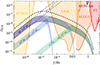Fig. 2. Mean GW energy density spectrum from massive BH mergers compared with the sensitivities of different experiments. The black dashed curve shows the case where all mergers of galaxies produce a GW signal for BHs heavier than 103 M⊙ (pBH = 1). The colored bands show the spectra from SMBHs heavier than 109 M⊙ (dark blue), from SMBHs in the range (106 M⊙, 109 M⊙); light blue), and from IMBHs with masses in the range 103 − 106 M⊙ (green), assuming a universal efficiency factor $p_{\mathrm{BH}}=0.{17}_{-0.08}^{+0.18}$. The shaded regions show the prospective sensitivities of IPTA30 (Chen et al. 2017; Kaiser & McWilliams 2021), LISA (LISA Collaboration 2017), AEDGE (El-Neaj et al. 2020; Badurina et al. 2021), AION-km (Badurina et al. 2020, 2021) and ET (Sathyaprakash et al. 2012).

We stress that the spectrum in Eq. (8), which is displayed in Fig. 2, does not necessarily correspond to a stochastic GW background as it does not distinguish between individual resolvable events and unresolvable events that would contribute to a GW background. The ${\mathrm{\Omega }}_{\mathrm{GW}}\propto f^{\frac{2}{3}}$ tail at low frequencies arises from nearly monochromatic signals generated by inspiralling BH binaries. Because of this, Ω_GW will fluctuate depending on the specific realization of the binary population, so the spectrum in Fig. 2 should be interpreted as the mean Ω_GW obtained by averaging over many potential realizations of the binary population. We return to the probability distribution of Ω_GW in the next subsection and in Appendix A.

The grey band in Fig. 2 was obtained by choosing a fixed value of p_BH so that the amplitude of the total GW spectrum from BH binaries matches the IPTA observations in the nHz range, which requires $p_{\mathrm{BH}}=0.{17}_{-0.08}^{+0.18}$. The colored bands show the contributions to the total IPTA spectrum from different ranges of the BH masses. In comparing the dark blue, light blue, and green bands, we can see that the largest contribution to the GW spectrum in the PTA window comes from M > 10⁹ M_⊙ SMBH binaries, consistent with earlier studies (Wyithe & Loeb 2003; Sesana et al. 2004, 2008, 2009; Enoki et al. 2004; Kelley et al. 2017a; Izquierdo-Villalba et al. 2021; Bécsy et al. 2022).

Some characteristics of these binaries are shown in Fig. 3. The left panel shows that the total masses are ≲10¹⁰, and the redshifts are typically 𝒪(1). The middle left panel shows that the typical masses increase with decreasing frequency and the middle right panel shows that the binary lifetimes are only weakly correlated with their emission frequencies, with lifetimes ≳10⁴ yr being generally favored. The right panel shows the GW strain from these binaries, together with the upper limit on continuous GW sources from NANOGrav 12.5 years data (Arzoumanian et al. 2023) and the projected sensitivity of IPTA30 (Chen et al. 2017; Kaiser & McWilliams 2021) at a signal-to-noise ratio of SNR = 8, which is similar to that expected for SKA (Janssen et al. 2015).

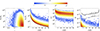Fig. 3. Distributions of the binary parameters for a sampling of the BH binary population with 0 < z < 3, 1 nHz < f < 30nHz and ${\mathcal{M}}_0>{10}^9{(f/\mathrm{nHz})}^{-\frac{4}{3}}$. The symmetric mass ratio is integrated with the lower bound η > 0.001. In the right panel, the black curve shows the NANOGrav 95% CL constraint on continuous GW sources (Arzoumanian et al. 2023) and the projected sensitivity of IPTA30 at SNR = 8.

Returning to Fig. 2, we see that the GW energy spectrum in the LISA frequency range is dominated by lighter BH binaries in the mass range of M ∈ (10⁶, 10⁹) M_⊙, shown in light blue, and the contribution in the AEDGE band is dominated by IMBHs with masses in the range of M ∈ (10³, 10⁶) M_⊙, shown in green. The low-frequency GW emissions from the early stages of the inspirals of these binaries also contribute in the lower-frequency bands, but these contributions are subdominant compared to the signals from higher-mass SMBH mergers⁴.

We recall that the estimated spectrum in Fig. 2 assumes a constant p_BH. Clearly, the relative contribution from binaries with lighter BH masses < 10⁹ M_⊙ could be enhanced (reduced) by increasing (decreasing) p_BH for these binaries. In order for mergers of BHs with masses in the range (10⁶, 10⁹) M_⊙ to dominate the PTA signal p_BH ≃ 1 would be required in this mass range, but even this maximal enhancement would be insufficient for mergers with M < 10⁶ M_⊙ to contribute significantly to the PTA signal. That said, we emphasize that the GW spectrum in either the LISA or AEDGE frequency range could reach the black dashed line if p_BH ≃ 1 in the relevant mass range, and could also be enhanced if Population III stars make a significant contribution to the BH spectrum. Conversely, the spectrum could be suppressed in these ranges if p_BH is smaller than the value that fits the PTA data.

3.2. Distribution of sources

The number of BH binaries at redshift z emitting in a given frequency band can be estimated from the time the binary spends in that frequency band, which gives (Sesana et al. 2008)

$$\begin{array}{c}\hfill \frac{\mathrm{d}N}{\mathrm{d}{\mathcal{M}}_z\mathrm{d}\eta \mathrm{d}z\mathrm{d}lnf}=\frac{\mathrm{d}\lambda }{\mathrm{d}{\mathcal{M}}_z\mathrm{d}\eta \mathrm{d}z}\left|\frac{\mathrm{d}\tau }{\mathrm{d}lnf}\right|,\end{array}$$(11)

where, assuming circular orbits and orbital decay via GW emission (Peters 1964), the coalescence time of an inspiralling binary emitting GWs with frequency (1 + z)f is⁵

$$\begin{array}{c}\hfill \tau (f)=\frac{5}{256{\pi }^{\frac{8}{3}}{\mathcal{M}}_z^{\frac{5}{3}}}{f}^{-\frac{8}{3}}.\end{array}$$(12)

We show in Fig. 4 the expected numbers of binaries with total masses of M ≥ M_min and mass ratios q ≥ 0.01 that emit GWs in several frequency bands in the range 1 nHz < f < 30 nHz (corresponding to the sensitivity ranges of PTAs). As seen in Fig. 2, SMBH binaries generate the dominant contribution to the GW signal in this frequency range. The fractions of the total GW signal in each frequency band that are generated by binaries with larger masses are indicated by the vertical dashed lines. For example, we see that almost 10⁵ (10²) binaries with M > 3 × 10⁹ M_⊙ generate 80% of the calculated GW signal in the 1 nHz < f < 3 nHz (10 nHz < f < 30 nHz) frequency band, whereas 50% of the calculated GW signal in the 3 nHz < f < 10 nHz band may be generated by just one source. These examples indicate that the expected signal, particularly in higher-frequency bins, may be comprised of a limited number of nearly monochromatic signals from heavy SMBH binaries ( > 10⁹ M_⊙), implying sizeable fluctuations around the smooth $f^{\frac{2}{3}}$ spectrum that would be obtained in the limit of a large population of heavy inspiralling binaries.

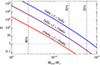Fig. 4. Expected number of SMBH binaries heavier than Mmin and with symmetric mass ratio η > 0.01 emitting GWs in the indicated frequency range for pBH = 0.17. The vertical dashed lines indicate the fractions of the total GW signal in each frequency band generated by binaries with larger masses.

In order to study the prospective SMBH binary population in the PTA band via a Monte Carlo approach, we generated realizations of the population from the probability density function of binaries emitting at a given frequency. We divide the frequency range into bins (f_j, f_j + 1) populated with N(f_j) binaries. A realization of the GW background from each bin can then be obtained as (see Eq. (A.6)):

$$\begin{array}{c}\hfill {\mathrm{\Omega }}_{\mathrm{GW}}(f_j)=\frac{1}{ln(f_{j+1}/f_j)}{\displaystyle \sum _{k=1}^{N(f_j)}{\mathrm{\Omega }}_{\mathrm{GW}}^{(1)}({\mathit{\theta }}_k),}\end{array}$$(13)

where the contribution from an individual binary emitting in this frequency band is given by

$$\begin{array}{c}\hfill {\mathrm{\Omega }}_{\mathrm{GW}}^{(1)}(\mathit{\theta })={\left|\frac{\mathrm{d}\tau }{\mathrm{d}lnf}\right|}^{-1}\frac{2\pi }{5}\frac{f^3{|\stackrel{\sim }{h}(f)|}^2}{{\rho }_c},\end{array}$$(14)

and θ ≡ {ℳ_z,zη,f} are parameters describing the binary. The number of binaries N(f_j) in this frequency bin is drawn from a Poisson distribution with the expectation value $\overline{N}(f_j)\equiv {\int }_{f_j}^{f_{j+1}}\text{d}N$ and the binary parameters are generated randomly according to the distribution

$$\begin{array}{c}\hfill p({\mathcal{M}}_z,\eta ,z,f)\propto \frac{\mathrm{d}N}{\mathrm{d}{\mathcal{M}}_z\mathrm{d}\eta \mathrm{d}z\mathrm{d}lnf}.\end{array}$$(15)

This is the expression that was used to calculate the distributions of binary parameters shown in Fig. 3 for a sampling with p_BH = 0.17 of 4 × 10⁵ SMBH binaries with redshifts 0 < z < 3, mass ratios η > 0.01, and GW frequencies 1 nHz < f < 30 nHz. We display only binaries with chirp mass ${\mathcal{M}}_0>{10}^9{(f/\mathrm{nHz})}^{-\frac{4}{3}}$, so that $\overline{N}(f_j)>\mathcal{O}({10}^4)$ for each 1 nHz frequency bin.

In order to generate the statistical distributions of Ω_GW, it is sufficient to consider a smaller set of parameters, and the distribution Eq. (11) for the full population can be reduced to a simpler distribution P(Ω⁽¹⁾, f) for individual sources ${\mathrm{\Omega }}_{\mathrm{GW}}^{(1)}$ emitting at a frequency f, which can be expressed via two one-parameter functions depending on the merger rate model, as discussed in Appendix A.

The upper left panel of Fig. 5 illustrates the frequency spectra found in 1600 Monte Carlo realizations of the SMBH binary population drawn from a statistical distribution similar to that shown in Fig. 3. The black solid curve shows the mean of the spectra, the grey bands show the 1σ and 2σ CL regions of the GW spectra, and the red line is the spectrum found in one representative realization. We note the importance of fluctuations, particularly at higher frequencies where fewer SMBH binaries contribute, with individual binaries becoming distinguishable at frequencies f ≳ 10 nHz. We find that the median spectrum, shown by the dashed line, has a somewhat lower slope than the analytic result shown as the green line. Although the numerically obtained mean spectrum (black), lies below the analytic expectation, it will approach it slowly if the number of Monte Carlo realizations is increased. The tendency of the mean spectrum to lie along the upper side of the 1σ CL range is due to the fact that the spectrum has a long tail at high values of Ω_GW generated by occasional nearby binaries: the median spectrum always lies within the 1σ CL range. All in all, consistently with earlier Monte Carlo studies of the GW signal (Sesana et al. 2008; Kocsis & Sesana 2011), we find that typical spectra tend to fall below the ${\mathrm{\Omega }}_{\mathrm{GW}}\propto f^{\frac{2}{3}}$ expectation in higher frequency bins, while a few bins display sharp peaks.

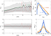Fig. 5. GW energy spectrum ΩGW and the fractional circular polarization 𝒫circ calculated from 1600 Monte Carlo realizations of the SMBH binary population. In the left panels, the black solid curve shows the mean and the gray bands the 68% and 95% CL regions of the Monte Carlo realizations, and the red curve corresponds to one of the realizations shown in Fig. 3. In the upper left panel the green line shows the mean GW energy density (8). The distributions of ΩGW and 𝒫GW at 1 nHz (blue) and at 30 nHz (orange) calculated from the Monte Carlo realizations are shown in the right panels. In the upper right panel, the dashed lines show $P\propto {\mathrm{\Omega }}^{-\frac{5}{2}}$, and in the lower right panel, the dashed curves show Gaussian fits to these distributions of width σ = 0.13 (blue) and σ = 0.23 (orange). In this figure, pBH = 0.17 is assumed.

As there are a finite number of sources, Eq. (8) is subject to statistical fluctuations, which arise mostly from the possibility of having a few strong sources nearby. To obtain an order-of-magnitude estimate, we focus on the closest binaries and ignore the redshift dependence. In this case, ${\mathrm{\Omega }}_{\mathrm{GW}}^{(1)}\propto D_L^{-2}$, by Eqs. (8) and (10), and the probability of finding an event at D_L is $P^{(1)}(D_L)\propto D_L^2$. Thus $⟨{\mathrm{\Omega }}_{\mathrm{GW}}^{(1)}⟩\propto {\int }_{D_{L,\min }}^{D_{L,\max }}\text{d}{D}_{L}P(D_L){\mathrm{\Omega }}_{\mathrm{GW}}^{(1)}\propto D_{L,\max }$, where, in this simplified approach, D_L,max is some large luminosity distance at which ${\mathrm{\Omega }}_{\mathrm{GW}}^{(1)}$ gets suppressed, and D_L,min is the distance to the nearest possible source. On the other hand, $⟨{({\mathrm{\Omega }}_{\mathrm{GW}}^{(1)})}^2⟩\propto 1/D_{L,\min }$. Therefore, we expect the mean of the GW signal to be determined by faraway sources, while the variance is set by a few close-by binaries. Moreover, we can estimate from P⁽¹⁾(D_L) that ${\mathrm{\Omega }}_{\mathrm{GW}}^{(1)}$ has a relatively flat power-law tail at large values,

$$\begin{array}{c}\hfill P^{(1)}(\mathrm{\Omega })\propto {\mathrm{\Omega }}^{-\frac{5}{2}},\text{when}\mathrm{\Omega }\to \infty .\end{array}$$(16)

Since the closest distance to massive BH binaries is constrained, this tail will be cut off at ${\mathrm{\Omega }}_{\mathrm{GW},\max }^{(1)}\propto D_{L,\min }^{-2}$. Even with this cutoff, the mean and the variance are still not very useful characteristics of the uncertainties, and we find it more illuminating to estimate the confidence intervals around the median value.

The upper right panel of Fig. 5 displays the distributions of Ω_GW at 1 nHz (blue) and at 30 nHz (orange) found in 1600 Monte Carlo realizations of the SMBH binary population. We note that the distributions at both frequencies have tails that approach the analytical result $P\propto {\mathrm{\Omega }}^{-\frac{5}{2}}$ (Eq. (16)), as indicated by the dashed lines. These tails exhibit explicitly why the mean (black solid) line in Fig. 5 tends to lie above the 68% CL band, while the median (gray dashed) line lies within it at all frequencies. We note that the overall shapes of the distributions resemble the analytic calculations shown in the left panel of Fig. A.1. In summary, even if a bin has a high number of contributing events (i.e., $\overline{N}\to \infty$), the distribution of Ω_GW does not converge to a Gaussian because it retains its ${\mathrm{\Omega }}_{\mathrm{GW}}^{-5/2}$ tail. Since the variance is not well behaved, we define the width of the distribution Δ_ΩGW as the width of the 68% confidence interval, as in Fig. 5. The width-to-mean ratio scales as:

$$\begin{array}{c}\hfill {\mathrm{\Delta }}_{{\mathrm{\Omega }}_{\mathrm{GW}}}/\langle {\mathrm{\Omega }}_{\mathrm{GW}}\rangle \propto {\overline{N}}^{-\frac{1}{3}},\end{array}$$(17)

when $\overline{N}\gg 1$, as is shown in Appendix A. This scaling is slower than the typical $1/\sqrt{\overline{N}}$ scaling predicted by the central limit theorem.

3.3. GW polarization

Recent studies have argued that the circular polarization of the signal can be used to estimate whether the SGWB comes from a handful of sources or a relatively large population of binaries (Kato & Soda 2016; Conneely et al. 2019; Hotinli et al. 2019; Belgacem & Kamionkowski 2020; Sato-Polito & Kamionkowski 2022; Valbusa Dall’Armi et al. 2023). We recall that the left and right circular GW polarization amplitudes from a binary with inclination angle θ are

$$\begin{array}{c}\hfill |h_{L,R}{(f)|}^2=\frac{1}{16}{(1\pm cos\theta )}^4{|h(f)|}^2,\end{array}$$(18)

where

$$\begin{array}{c}\hfill |h(f)|=\frac{4{\mathcal{M}}_z^{\frac{5}{3}}}{D_L}{(\pi f)}^{\frac{2}{3}}\end{array}$$(19)

is the maximal GW strain from an inspiralling binary, and the gravitational Stokes parameters are defined by

$$\begin{array}{c}\hfill \begin{array}{cc}\hfill I(f)& =|h_L{(f)|}^2+{|h_R(f)|}^2,\hfill \\ \hfill V(f)& =|h_L{(f)|}^2-{|h_R(f)|}^2.\hfill \end{array}\end{array}$$(20)

The fractional amount of circular polarization of the SGWB can be characterized by the quantity

$$\begin{array}{c}\hfill {\mathcal{P}}_{\mathrm{circ}}(f)=\frac{{\sum }_i{V}_i(f)}{{\sum }_i{I}_i(f)},\end{array}$$(21)

where the sums are over all binaries in a fixed frequency range.

If the GW signal is dominated by a single source, then 𝒫_circ depends only on the inclination angle and large circular polarizations are preferred, with 𝒫_circ > 0.87(0.2) at the 68% CL (95% CL). On the other hand, if the GW signal is dominated by several (N_dom ≳ 10) sources of comparable strengths, then the 𝒫_circ(f) will be approximately Gaussian with a width determined by fluctuations in σ_V. Since σ_V/⟨I⟩_θ = 1.17 for a single source, we can estimate that (see Appendix A for details)

$$\begin{array}{c}\hfill {\sigma }_{{\mathcal{P}}_{\mathrm{circ}}}\approx {\sigma }_V/{⟨I⟩}_{\theta }\approx 1.17/\sqrt{N_{\mathrm{dom}}}.\end{array}$$(22)

The lower-left panel of Fig. 5 illustrates the distributions of the circular polarization 𝒫_circ(f) found in the sample of 1600 Monte Carlo realizations of the SMBH binary population with M > 10⁹ M_⊙ and η > 0.01 whose frequency spectra were illustrated in Fig. 5. We see that the mean value of 𝒫_circ(f)≈0, as expected, but large statistical fluctuations are possible even at the 1σ level. This phenomenon is visible in the red curve, which shows results from one of the Monte Carlo realizations. The large fluctuations reflect the fact that the observable GW spectrum could be due to a very limited number of sources, particularly at higher frequencies.

The lower-right panel of Fig. 5 displays the distributions of 𝒫_circ at 1 nHz (blue) and at 30 nHz (orange) found in 1600 Monte Carlo realizations of the SMBH binary population. We note that the statistical distribution is indeed broader at the higher frequency, as expected. The dashed curves are Gaussian fits to polarization distributions with widths σ = 0.13 (blue) and σ = 0.23 (orange). These fits are very accurate as also demonstrated in the right panel of Fig. A.1.

As the variance of the circular polarization of the signal depends on the number of binaries that dominate the signal, it would be suppressed if the merger rate of the heaviest binaries were suppressed, which could be the case if p_BH is not universal. By suppressing p_BH, for instance, at M > 10⁹ M_⊙ and enhancing p_BH for 10⁹ M_⊙ > M > 10⁶ M_⊙, we can accommodate the IPTA common-spectrum effect. In this case, the GW energy spectrum Ω_GW becomes smoother and approaches the naive ${\mathrm{\Omega }}_{\mathrm{GW}}\propto f^{\frac{2}{3}}$ behavior while suppressing the circular polarization 𝒫_circ. Moreover, in this case, p_BH for the lighter binaries would be enhanced, which would increase the number of signals in the sensitivity range of LISA and possibly AEDGE.

3.4. Prospects for future GW observatories

As discussed earlier, BH binaries can generate two qualitatively distinct classes of signal: long, nearly monochromatic signals from the slowly-evolving inspiralling phase and relatively short signals from the merger and ringdown. The detections of these two types of sources need to be considered separately.

The number of detectable nearly monochromatic GW signals that arise from inspiralling BH binaries is

$$\begin{array}{c}\hfill N_{\mathrm{insp}}={\displaystyle {\int }_{\mathcal{T}+{\tau }_{\min }}^{\infty }\mathrm{d}\tau \int \mathrm{d}\lambda p_{\det }\left[\frac{{\mathrm{SNR}}_c}{\mathrm{SNR}(\tau ,z)}\right],}\end{array}$$(23)

where we account only for binaries whose coalescence time τ is longer than τ_min = 1 day and we estimate the SNR for a detector characterized by the noise power spectrum S_n(f) as

$$\begin{array}{c}\hfill \mathrm{SNR}(\tau ,z)=\sqrt{{\displaystyle {\int }_0^{\mathcal{T}}}\mathrm{d}t\frac{{2|h(\tau -t,z)|}^2}{S_n(f(\tau -t,z))}}.\end{array}$$(24)

The optimal time-dependent inspiral strain |h(t)| = |h(f(t))| is given by Eq. (19) and the GW frequency as a function of time is given by Eq. (12). Analogously, the expected number of BH binary merger events is

$$\begin{array}{c}\hfill N_{\mathrm{merg}}=\mathcal{T}{\displaystyle \int }\mathrm{d}\lambda p_{\det }\left[\frac{{\mathrm{SNR}}_c}{\mathrm{SNR}(z)}\right],\end{array}$$(25)

where

$$\begin{array}{c}\hfill \mathrm{SNR}(z)=\sqrt{{\displaystyle {\int }_{f({\tau }_{\min })}^{\infty }}\mathrm{d}f\frac{4|\stackrel{\sim }{h}{(f)|}^2}{S_n(f)}}.\end{array}$$(26)

The cut at f(τ_min) here implies that we only consider the SNR only from the last day of the signal. In both cases, the detection probability p_det accounts for the detector’s antenna patterns and includes the average over the binary inclination, sky location, and polarization (Finn & Chernoff 1993; Gerosa et al. 2019), the noises S_n include the foregrounds from stellar mass BH binaries and white dwarf binaries (see e.g., Lewicki & Vaskonen 2021). Furthermore, we used SNR_c = 8 for the detection threshold and 𝒯 = 1 yr for the observation time.

In the monochromatic limit, Eq. (24) is simplified to $\mathrm{SNR}=|h(f)|\sqrt{2\mathcal{T}/S_n(f)}$. Using this, we can convert the prospected noise S_n(f) of IPTA30 to a lower bound on the strain |h(f)| for which the SNR exceeds the detection threshold. As indicated by the very long coalescence times in the middle right panel of Fig. 3, the signals in the IPTA30 band can be adequately approximated as monochromatic. In the right panel of Fig. 3 the dashed black curve shows the GW strain |h(f)| that for 20 year observation time with IPTA30 gives SNR = 8. We see that IPTA30 can potentially resolve several, 𝒪(10), monochromatic GW signals from SMBH binaries.

At higher frequencies, f > 10⁻⁶ Hz, we find that LISA is the only detector capable of measuring the near-monochromatic sources arising in the early stages of the inspiral phase, namely, more than one day from the beginning of the merger phase. It is clear that AEDGE is not able to observe these near-monochromatic sources because the coalescence time of binaries heavier than 10³ M_⊙ is less than a day when they enter the AEDGE sensitivity window⁶. Figure 6 illustrates the prospects to detect the inspiral signals with LISA. The shading in the panels correspond to the number of events whose parameters fall within each rectangular bin. The distribution peaks below ℳ₀ = 10⁴ M_⊙ reflecting the binary population, that increases towards lower masses, and the cut-off at 10³ M_⊙. Similarly, because the GW signal (Eq. (10)) from inspirals does not explicitly depend on η, the η distribution in the right panel of Fig. 6 arises solely from the binary population. The binary merger rate peaks at 4 < z < 6 (see Fig. 1) but LISA cannot spot the majority of the binaries beyond z ∼ 4.

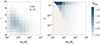Fig. 6. Expected numbers of near-monochromatic GW signals generated more than a day before the merger that would be detectable in a year of LISA observation, as functions of the chirp mass ℳ0 and redshift z (left panel) and of the chirp mass and symmetric mass ratio η (right panel). The merger rates assume the abundance of IMBHs described by Eq. (6) for BHs heavier than 103 M⊙ and a universal merger efficiency factor of pBH = 0.17 inferred from IPTA data, as discussed in the text.

We find that, at z < 10, there are a total of 𝒪(10⁷) near-monochromatic sources in the frequency range of 10⁻⁵ Hz < f < 0.1 Hz⁷. As only a small fraction of these can be resolved by LISA, we expect that the rest constitute a significant stochastic GW background. It should be noted that the potential redshift dependence of p_BH introduces additional uncertainties in the merger rate at higher redshifts (z ≳ 3), which is not well probed by the PTA measurements. We leave a detailed study of this background and its detectability with LISA for future work.

Figure 7 illustrates AEDGE and LISA prospects for observing GW events from BHs less than a day after the merger. The expected total number of detectable events is slightly larger for LISA than for AEDGE. Due to the different frequency ranges, LISA can spot heavier binaries, ℳ₀ > 10⁴ M_⊙, while AEDGE can see lighter binaries, ℳ₀ < 2 × 10³ M_⊙. LISA could (in principle) detect even heavier mergers, namely, of ℳ₀ ≲ 10⁸ M_⊙, but since such mergers are so rare it is unlikely that LISA will see any mergers above 10⁶ M_⊙. The expected number of detectable mergers peaks at 4 < z < 6 for both of the experiments. For AEDGE, the z distribution of the detectable mergers reflects the binary merger rate (see Fig. 1) while for LISA the z distribution peaks at slightly lower z because the SNR of ℳ₀ ∼ 10⁴ binaries for LISA is not as high as it is for AEDGE. The lower panels show that, for all detectors, the BH mass ratio peaks at the highest values. For AION-km and ET we find that the total expected number of events per year is less than three.

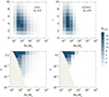Fig. 7. Expected numbers of detectable GW events generated during the last day before the merger in a year of observation by LISA (left panels) and AEDGE (right panels) as functions of the chirp mass ℳ0 and redshift z (upper panels) and of chirp mass and symmetric mass ratio η (lower panels). The merger rates assume the abundance of IMBHs described by Eq. (6) for BHs heavier than 103 M⊙ and a universal merger efficiency factor of pBH = 0.17 inferred from the IPTA data.

We note that most of the IMBH events detectable by AEDGE during the last day prior to the merger (see the left panels in Fig. 7) will also have been detected by LISA during the previous infall stage, as seen in Fig. 6. This opens up prospects for using LISA data to predict when and in what direction AEDGE will observe IMBH mergers, sharpening tests of general relativity and giving advance warnings for searches for possible multi-messenger signals.

We caution that there are observational uncertainties in the low mass cut-off in Eq. (6), due to the difficulty of measuring very faint active galactic nuclei (AGNs) or inactive BHs in dwarf galaxies. As mentioned above, surveys such as eRASS and AMUSE (Miller et al. 2015) are already constraining this low-mass region and are compatible with the assumed cut-off, although a heavier mass cut-off may be favored (Chadayammuri et al. 2023). This could easily be achieved in models with modified initial fluctuation spectra (Hütsi et al. 2023).

The cut-off mass is tightly related to the SMBH formation mechanism since a BH in the halo centre cannot be lighter than the seed that originated the growth. For a full review, we refer to Volonteri et al. (2021). In this sense, the cut-off we have considered assumes the existence of some light seeds, which augment the possible GW signal. Independently of the growth through halo merging, IMBHs can also be born inside dense stellar media like nuclear and globular star clusters. The growth from stellar masses happens because of repeated encounters inside these dense environments. Estimating the GW emission from such encounters is an active field of research (Fragione & Kocsis 2018; Fragione et al. 2019; Fragione & Loeb 2023) and their signals may contribute significantly to the expected number of IMBH mergers.

4. Conclusions

Here, we describe the results from a model for the PTA nHz common-process signal based on a simulation of massive BH mergers. The magnitude of the signal depends on the merger probability, p_BH, which is a product of the probabilities that a pair of halos contain massive BHs and the probability that they will merge. We sidestepped the considerable uncertainties in modeling these probabilities by fitting a mass-independent value of p_BH to the PTA signal, finding p_BH = 0.17, with a factor of two uncertainty. With this assumption, the dominant contribution to the PTA signal is made by mergers with total masses > 10⁹ M_⊙ and about 10% from masses < 10⁹ M_⊙. The PTA mergers would have redshifts 𝒪(1) and have mass asymmetries ≳10.

The number of mergers contributing most of the PTA signal at frequencies 𝒪(10) nHz is limited. Consequently, the frequency spectrum becomes quite irregular, the spectral index may deviate from the analytic value of 2/3, individual mergers may be distinguished, and there may be detectable circular polarization. These will be interesting targets for future experiments in the nHz range, including PTAs and SKA.

Assuming the same mass-independent value of p_BH as for the PTA signal, there would be observable signals from mergers with total masses ∈(10³, 10⁶) M_⊙ in the LISA experiment and from mergers with total masses ∈(10³, 10⁵) M_⊙ in the AEDGE experiment. Data from these experiments will be able to check the accuracy of the constancy of p_BH. In principle, their signals could be even larger than our estimates if p_BH is closer to unity for masses below the PTA range, or if there is a significant GW contribution seeded by Population III stars. However, a lower value for p_BH and, hence, a lower event rate cannot be excluded.

Acknowledgments

This work was supported by European Regional Development Fund through the CoE program grant TK133 and by the Estonian Research Council grants PRG803 and PSG869. The work of J.E. was supported by the United Kingdom STFC Grant ST/T000759/1. The work of V.V. was supported by the European Union’s Horizon Europe research and innovation programme under the Marie Skłodowska-Curie grant agreement No. 101065736.

References

Appendix A: Statistics of the GW energy spectrum and circular polarization

A.1. Distribution of Ω_GW(f)

The GW energy spectrum arising from a population of BH binaries can be expressed as the sum of the contributions from individual binaries. We first consider the contribution to Ω_GW coming from a single inspiralling binary:

$$\begin{array}{c}\hfill {\mathrm{\Omega }}_{\mathrm{GW}}^{(1)}(\mathit{\theta })={\left|\frac{\mathrm{d}\tau }{\mathrm{d}lnf}\right|}^{-1}\frac{2\pi }{5}\frac{f^3{|\stackrel{\sim }{h}(f)|}^2}{{\rho }_c},\end{array}$$(A.1)

where θ ≡ {ℳ_z,z,f} are parameters describing the binary. The GW energy spectrum arising from the inspiralling binary population (or any of its subpopulations) arises from the sum of nearly monochromatic components

$$\begin{array}{c}\hfill {\mathrm{\Omega }}_{\mathrm{GW}}(f)\approx {\displaystyle \sum _i{\mathrm{\Omega }}_{\mathrm{GW}}^{(1)}({\mathit{\theta }}_i)\delta (lnf/f_i).}\end{array}$$(A.2)

This approximation is valid as long as the change in frequency over the observation period is smaller than the spectral resolution. The parameters θ_i as well as ${\mathrm{\Omega }}_{\mathrm{GW}}^{(1)}$ are independent and identically distributed. Thus, the statistical properties of Ω_GW(f) can be inferred from the distribution of ${\mathrm{\Omega }}_{\mathrm{GW}}^{(1)}(f)$, which is given by

$$\begin{array}{c}\hfill \begin{array}{cc}\hfill P^{(1)}(\mathrm{\Omega }|f)& =\frac{1}{n(f)}{\displaystyle \int }\mathrm{d}\lambda \left|\frac{\mathrm{d}\tau }{\mathrm{d}lnf}\right|\delta (\mathrm{\Omega }-{\mathrm{\Omega }}_{\mathrm{GW}}^{(1)})\hfill \\ \hfill & =\frac{\mathcal{F}(\mathrm{\Omega }{f}^{-\frac{10}{3}})}{f{\mathrm{\Omega }}^{\frac{3}{2}}n(f)},\hfill \end{array}\end{array}$$(A.3)

where we define the following function:

$$\begin{array}{c}\hfill \begin{array}{cc}\hfill \mathcal{F}(x)\equiv {\displaystyle \int }\mathrm{d}z& \mathrm{d}\eta [\frac{\partial \lambda ({\mathcal{M}}_z,z)}{\partial {\mathcal{M}}_z\partial \eta \partial z}\hfill \\ \hfill & \times \frac{{\mathcal{M}}_z}{16\sqrt{10{\rho }_c}{D}_L}{]}_{{\mathcal{M}}_z=\frac{1}{\pi }{\left(\frac{5\pi }{8}{D}_L^3{\rho }_{c}x\right)}^{\frac{3}{10}}}\hfill \end{array}\end{array}$$(A.4)

and the spectral source density:

$$\begin{array}{c}\hfill n(f)\equiv {\displaystyle \int }\mathrm{d}{\mathcal{M}}_z\mathrm{d}\eta \mathrm{d}z\frac{\mathrm{d}N}{\mathrm{d}{\mathcal{M}}_z\mathrm{d}\eta \mathrm{d}z\mathrm{d}lnf}.\end{array}$$(A.5)

We see that, for circular inspiralling binaries, the four-parameter distribution (11) can be reduced to two functions of a single parameter. Further reductions are unlikely, as these functions depend on the model of the binary merger rate, which we assume to stem from the merger rate of galaxies.

The average energy spectrum in a frequency bin (f_j, f_j + 1) can be obtained from

$$\begin{array}{c}\hfill \begin{array}{cc}\hfill {\mathrm{\Omega }}_{\mathrm{GW}}(f_j)& \equiv \frac{1}{ln(f_{j+1}/f_j)}{\displaystyle {\int }_{f_j}^{f_{j+1}}{\mathrm{\Omega }}_{\mathrm{GW}}(\mathit{\theta };f)\mathrm{d}lnf}\hfill \\ \hfill & =\frac{1}{ln(f_{j+1}/f_j)}{\displaystyle \sum _{i=1}^{N(f_j)}{\mathrm{\Omega }}_{\mathrm{GW},i}^{(1)},}\hfill \end{array}\end{array}$$(A.6)

where the number of binaries N(f_j) is drawn from a Poisson distribution with the expected value,

$$\begin{array}{c}\hfill \overline{N}(f_j)={\displaystyle {\int }_{f_j}^{f_{j+1}}\mathrm{d}lnfn(f),}\end{array}$$(A.7)

and the ${\mathrm{\Omega }}_{\mathrm{GW},i}^{(1)}$ are drawn from a random distribution $P^{(1)}(\mathrm{\Omega },f)=P^{(1)}(\mathrm{\Omega }|f)n(f)/\overline{N}(f_j)$ with f ∈ (f_j, f_j + 1). In the following, we suppress f_j.

The moment generating function of Ω_GW is given by:

$$\begin{array}{c}\hfill \begin{array}{cc}\hfill M_{{\mathrm{\Omega }}_{\mathrm{GW}}}(s)& \equiv ⟨exp\left(s{\mathrm{\Omega }}_{\mathrm{GW}}\right)⟩\hfill \\ \hfill & ={\displaystyle \sum _{N\ge 0}{p}_N\prod _{i=1}^N\langle exp\left(s{\mathrm{\Omega }}_{\mathrm{GW}}^{(1)}\right)\rangle }\hfill \\ \hfill & ={\displaystyle \sum _{N\ge 0}\frac{{\overline{N}}^N}{N!}{e}^{-\overline{N}}{\left(M_{{\mathrm{\Omega }}_{\mathrm{GW}}^{(1)}}(s)\right)}^{\overline{N}}}\hfill \\ \hfill & =exp\left[\overline{N}(M_{{\mathrm{\Omega }}_{\mathrm{GW}}^{(1)}}(k)-1)\right].\hfill \end{array}\end{array}$$(A.8)

Thus, the cumulant generating function of Ω_GW(f_j), that is,

$$\begin{array}{c}\hfill \begin{array}{cc}\hfill K_{{\mathrm{\Omega }}_{\mathrm{GW}}}(s)& \equiv ln{M}_{{\mathrm{\Omega }}_{\mathrm{GW}}}(s)\hfill \\ \hfill & ={\displaystyle {\int }_{f_j}^{f_{j+1}}\mathrm{d}N[exp(s{\mathrm{\Omega }}_{\mathrm{GW}}^{(1)})-1].}\hfill \end{array}\end{array}$$(A.9)

is proportional to the generating function of $M_{{\mathrm{\Omega }}_{\mathrm{GW}}^{(1)}}(s)$, implying that the nth cumulant of Ω_GW is

$$\begin{array}{c}\hfill \begin{array}{c}\hfill {\kappa }_n[{\mathrm{\Omega }}_{\mathrm{GW}}]=\overline{N}⟨{({\mathrm{\Omega }}_{\mathrm{GW}}^{(1)})}^n⟩={\displaystyle {\int }_{f_j}^{f_{j+1}}\mathrm{d}N{({\mathrm{\Omega }}_{\mathrm{GW}}^{(1)})}^n.}\end{array}\end{array}$$(A.10)

Therefore, the mean κ₁(Ω_GW)≡⟨Ω_GW⟩ matches the expectation value given in Eq. (8), while the variance,

$$\begin{array}{c}\hfill {\kappa }_2({\mathrm{\Omega }}_{\mathrm{GW}})\equiv ⟨{(\delta {\mathrm{\Omega }}_{\mathrm{GW}})}^2⟩=\overline{N}⟨{({\mathrm{\Omega }}_{\mathrm{GW}}^{(1)})}^2⟩\end{array}$$(A.11)

is divergent due to the long $P^{(1)}(\mathrm{\Omega })\propto {\mathrm{\Omega }}^{-\frac{5}{2}}$ tail (16), unless a minimal distance to the closest BH binary is imposed. In particular, as we will demonstrate briefly, this long tail is preserved in the distribution of Ω_GW, i.e., the higher cumulants are not diminished when summing several instances of $P^{(1)}(\mathrm{\Omega })\propto {\mathrm{\Omega }}^{-\frac{5}{2}}$.

The moment-generating function M_ΩGW(−s) is a Laplace transform of the probability distribution. Thus as an alternative to the Monte Carlo approach adopted in the main text, the probability distribution of Ω_GW(f_j) can be obtained by an inverse Laplace transform of the moment generating function given in Eq. (A.8). It can be expressed as

$$\begin{array}{c}\hfill \begin{array}{cc}\hfill P({\mathrm{\Omega }}_{\mathrm{GW}})& =\frac{1}{2\pi \overline{N}}{\displaystyle {\int }_{-\infty }^{\infty }\mathrm{d}s{e}^{is{\mathrm{\Omega }}_{\mathrm{GW}}/\overline{N}}\times }\hfill \\ \hfill & \times exp\left(\overline{N}\langle exp(-is{\mathrm{\Omega }}_{\mathrm{GW}}^{(1)}/\overline{N})-1\rangle \right),\hfill \end{array}\end{array}$$(A.12)

where the average is taken over the single event distribution P⁽¹⁾.

A.1.1. The large N limit. –

The central limit theorem (and Eq. (A.11)) dictates that when N → ∞, then the distribution (A.6) should approach a Gaussian with its relative width scaling as ${\sigma }_{{\mathrm{\Omega }}_{\mathrm{GW}}}/⟨{\mathrm{\Omega }}_{\mathrm{GW}}⟩\propto 1/\sqrt{N}$. However, this is not the case when the second cumulant diverges. Considering a generic distribution with a tail (droping the "GW" subindex for the sake of brevity):

$$\begin{array}{c}\hfill P^{(1)}(\mathrm{\Omega })\stackrel{\mathrm{\Omega }\to \infty }{\sim }C{\mathrm{\Omega }}^{-\frac{5}{2}},\end{array}$$(A.13)

where C is a constant. The second moment ⟨Ω²⟩ diverges. We assume that the small Ω behavior is such that the first moment ${\overline{\mathrm{\Omega }}}^{(1)}\equiv ⟨{\mathrm{\Omega }}^{(1)}⟩$ is finite. The $\overline{N}\to \infty$ asymptotic of the average in Eq. (A.12) can then be computed by separating it into the mean and a term for which the expectation value can be determined by approximating the distribution by its tail (A.13):

$$\begin{array}{cc}& \overline{N}\langle exp(-is\frac{{\mathrm{\Omega }}^{(1)}}{\overline{N}})-1\rangle \hfill \\ \hfill =& -is{\overline{\mathrm{\Omega }}}^{(1)}+\overline{N}\langle exp(-is\frac{{\mathrm{\Omega }}^{(1)}}{\overline{N}})-1+is\frac{{\mathrm{\Omega }}^{(1)}}{\overline{N}}\rangle \hfill \\ \hfill \stackrel{N\to \infty }{\sim }& -is{\overline{\mathrm{\Omega }}}^{(1)}+e^{i\pi \frac{3}{4}}\frac{\sqrt{\pi }4C}{3\sqrt{\overline{N}}}{s}^{\frac{3}{2}}.\hfill \end{array}$$(A.14)

In summary, the N → ∞ distribution asymptotes to

$$\begin{array}{c}\hfill \begin{array}{cc}\hfill P(\mathrm{\Omega })& \approx {(C\overline{N})}^{-\frac{2}{3}}\mathcal{P}\left({(C\overline{N})}^{-\frac{2}{3}}(\mathrm{\Omega }-\overline{\mathrm{\Omega }})\right),\hfill \end{array}\end{array}$$(A.15)

where $\overline{\mathrm{\Omega }}\equiv \overline{N}{\overline{\mathrm{\Omega }}}^{(1)}$ denotes the expectation value of Ω and

$$\begin{array}{c}\hfill \begin{array}{c}\hfill \mathcal{P}\left(x\right)\equiv \mathrm{Re}\frac{e^{i\pi /6}}{\pi }{\displaystyle {\int }_0^{\infty }\mathrm{d}sexp(i{e}^{i\pi /6}xs-\frac{4\sqrt{\pi }}{3}{s}^{\frac{3}{2}})}\end{array}\end{array}$$(A.16)

is a universal function that is independent of the single event distribution – all information about the latter enters through ${\overline{\mathrm{\Omega }}}^{(1)}$ and C. This limiting case reveals a few crucial features:

1. Since 𝒫(x)∼x^−5/2 when x → ∞, the power-law behavior of the tail is preserved in the large $\overline{N}$ limit:

   $$\begin{array}{c}\hfill P(\mathrm{\Omega })\stackrel{\mathrm{\Omega }\gg \overline{\mathrm{\Omega }}}{\approx }\frac{C\overline{N}}{{(\mathrm{\Omega }-\overline{\mathrm{\Omega }})}^{\frac{5}{2}}}.\end{array}$$(A.17)

2. When the number of contributing events N is increased by a factor of A to AN, the distribution evolves as

   $$\begin{array}{c}\hfill P^{(AN)}(\mathrm{\Omega })=A^{-\frac{2}{3}}{P}^{(N)}(A^{-\frac{2}{3}}(\mathrm{\Omega }-{\overline{\mathrm{\Omega }}}^{(AN)})+{\overline{\mathrm{\Omega }}}^{(N)}).\end{array}$$(A.18)

3. Although the variance diverges, we can define the width of the distribution Δ_Ω ≡ Ω₊ − Ω₋ from the confidence interval (Ω₋, Ω₊) centred around, e.g., the median. Eq. (A.18) then implies the scaling

   $$\begin{array}{c}\hfill {\mathrm{\Delta }}_{\mathrm{\Omega }}\propto {\overline{N}}^{2/3}.\end{array}$$(A.19)

   So, the relative width ${\mathrm{\Delta }}_{\mathrm{\Omega }}/\overline{\mathrm{\Omega }}$ will approach zero, but at a slower pace than when the central limit theorem applies.

4. Using the method of steepest decent, we find that

   $$\begin{array}{c}\hfill \mathcal{P}\left(x\right)\stackrel{\mathrm{\Omega }\ll \overline{\mathrm{\Omega }}}{\approx }\frac{\sqrt{\overline{\mathrm{\Omega }}-\mathrm{\Omega }}}{2\pi C\overline{N}}{e}^{-\frac{{(\overline{\mathrm{\Omega }}-\mathrm{\Omega })}^3}{12\pi {(C\overline{N})}^2}},\end{array}$$(A.20)

   implying values smaller than the mean, that is $\mathrm{\Omega }<\overline{\mathrm{\Omega }}$, are much less likely than for Gaussian distributions, as they are suppressed by an exponent of a cube.

As an illustration, we consider a population of sources for which individual signals follow the simple long-tailed distribution

$$\begin{array}{c}\hfill P^{(1)}(\mathrm{\Omega })\propto {\mathrm{\Omega }}^{-\frac{5}{2}}\theta (\mathrm{\Omega }-{\mathrm{\Omega }}_{min}),\end{array}$$(A.21)

which mimics the statistics of Ω_GW from a realistic BH population found in section 3.2. In Fig. A.1, we show the resulting distributions of $\mathrm{\Omega }/\overline{\mathrm{\Omega }}$ if the signal consists of 10, 100, and 10⁵ sources. The mean is given by $\overline{\mathrm{\Omega }}\equiv 3N{\mathrm{\Omega }}_{\min }$. The distribution is computed by generating random realizations of the source populations (shown by points) and by using (A.12) (shown by solid lines). These two approaches are in excellent agreement. As expected, one can observe that the total signal will inherit the long Ω^−5/2 tail from the distribution of individual sources (shown by the dashed line). At large Ω, the tail approaches Eq. (A.17) in all cases, while the asymptotic (A.15) works well for N = 10⁵, but predicts a slightly too wide peak for N ≤ 10⁵. As predicted, the peak gets narrower and moves closer to the expectation value, when N is increased. We note, however, that although the shape of the simplified distribution in Fig. A.1 resembles the distribution in Fig. 5 obtained from a model of the heavy BH binary population, the shape around the peak in the latter depends also on the z dependence and the binary mass distribution.

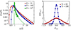Fig. A.1. Distributions of the total signal strengths from 1, 10, 100, and 105 sources whose independent signal strengths have identical ${\mathrm{\Omega }}^{-\frac{5}{2}}$ tails (left). Distribution of 𝒫circ for 1, 10 and 100 identical sources (right). The dashed line shows the distribution from a single source, the solid lines show the analytic estimates, and the distributions obtained from an explicit Monte Carlo analysis are shown by the points.

A.2. Distribution of 𝒫_circ

Considering now the distribution of the circular polarization

$$\begin{array}{c}\hfill {\mathcal{P}}_{\mathrm{circ}}\equiv \frac{{\sum }_{i=1}^N{V}_i}{{\sum }_{i=1}^N{I}_i},\end{array}$$(A.22)

which depends on the distribution and number N of sources. We denote the contributions from individual sources by V_i, I_i given by Eqs. (18-20). As above, we are working in a fixed frequency bin and, thus, suppressing the frequency dependence in the arguments of the functions.

The polarization will vanish on average, that is, at ⟨𝒫_circ⟩ = 0, but polarization measurements can provide information from the size of the deviation from that expectation. For a single dominant source, the contribution from the amplitude drops out and we find

$$\begin{array}{c}\hfill {\mathcal{P}}_{\mathrm{circ}}=\frac{4c_{\theta }(1+c_{\theta }^2)}{1+6c_{\theta }^2+c_{\theta }^4},\end{array}$$(A.23)

where c_θ ≡ cos(θ). The corresponding probability distribution is shown as the dashed curve in Fig. A.1 and can be seen to be dominated by the region |𝒫_circ|≈1.

If the signal is dominated by several sources, the analytic treatment of 𝒫_circ is complicated due to correlations between V and I. The mean and variance of I and V are given by

$$\begin{array}{c}\hfill \begin{array}{cc}\hfill ⟨I⟩& =\frac{4}{5}{⟨|h|}^2⟩,⟨V⟩=0,\hfill \\ \hfill ⟨\delta I^2⟩& =\frac{284}{315}{⟨(\delta |h|}^2{)}^2⟩,⟨\delta V^2⟩=\frac{92}{105}{⟨(\delta |h|}^2{)}^2⟩,\hfill \end{array}\end{array}$$(A.24)

where we used the fact that the inclination is independent of other parameters of the binary and the fluctuations in |h|² are computed as in (A.11). The latter is expected to be large. To estimate the fluctuations in 𝒫_circ in the limit when the number of sources is large, we first assume that I can be replaced by its average over inclinations ⟨I⟩_θ ≡ (4/5)∑_i|h_i|², but not over signal strengths, so that

$$\begin{array}{c}\hfill {\mathcal{P}}_{\mathrm{circ}}\approx V/{⟨I⟩}_{\theta }\equiv {\displaystyle \sum _{i=1}^N{p}_i{f}_V(c_{\theta ,i}),}\end{array}$$(A.25)

where p_i ≡ (4/5)|h_i|²/⟨I⟩_θ ∈ [0, 1] is the fractional contribution to the signal from source i and $f_V(c_{\theta })=(5/4)c_{\theta }(1+c_{\theta }^2)$ contains the inclination dependence of V. In this way, it is possible to contain the effect of the large fluctuations in ⟨I⟩_θ in the random fractions p_i, which vary only in the range [0, 1]. We find:

$$\begin{array}{c}\hfill ⟨\delta {\mathcal{P}}_{\mathrm{circ}}^2⟩=\frac{115}{84}N⟨|p_i{|}^2⟩.\end{array}$$(A.26)

We note that N⟨|p_i|²⟩ takes values in the range [1/N, 1] and could be interpreted as a measure of the effective number of dominant sources 1/N_dom. For instance, in the limiting case where the signal is sourced by N binaries that contribute equally, that is, p_i = 1/N, we would obtain

$$\begin{array}{c}\hfill {\sigma }_{{\mathcal{P}}_{\mathrm{circ}}}=1.17/\sqrt{N},\end{array}$$(A.27)

as also stated in Eq. (22). In the right panel of Fig. A.1, approximate Gaussian distributions with a width given by (A.27) and shown as solid lines are compared to distributions obtained from explicitly generated random populations of 𝒫_circ arising from exactly 10 and 100 sources of equal strength (shown by points). We see an excellent agreement between the naive Gaussian approximation and the Monte Carlo estimate already for N = 10.

Finally, we remark that the approximation (A.25) above can be improved by expanding 𝒫_circ in δI ≡ I − ⟨I⟩_θ, that is, 𝒫_circ = V/⟨I⟩_θ(1 − δI/⟨I⟩_θ + …). This allows us to account for correlations between V and δI, for instance, when computing the variance (A.26),

$$\begin{array}{c}\hfill ⟨\delta {\mathcal{P}}_{\mathrm{circ}}^2⟩=\frac{115}{84}N⟨|p_i{|}^2⟩-\frac{2855}{1386}N⟨|p_i{|}^3⟩+\dots \end{array}$$(A.28)

The corrections arising from higher powers of δI/⟨I⟩_θ are suppressed by increasing powers of 1/N.

All Figures

	Fig. 1. BH merger rates calculated as functions of the redshift z in three ranges of the total merging BH mass M and normalized relative to the merger probability pBH discussed in the text.
In the text

Fig. 2. Mean GW energy density spectrum from massive BH mergers compared with the sensitivities of different experiments. The black dashed curve shows the case where all mergers of galaxies produce a GW signal for BHs heavier than 103 M⊙ (pBH = 1). The colored bands show the spectra from SMBHs heavier than 109 M⊙ (dark blue), from SMBHs in the range (106 M⊙, 109 M⊙); light blue), and from IMBHs with masses in the range 103 − 106 M⊙ (green), assuming a universal efficiency factor $p_{\mathrm{BH}}=0.{17}_{-0.08}^{+0.18}$. The shaded regions show the prospective sensitivities of IPTA30 (Chen et al. 2017; Kaiser & McWilliams 2021), LISA (LISA Collaboration 2017), AEDGE (El-Neaj et al. 2020; Badurina et al. 2021), AION-km (Badurina et al. 2020, 2021) and ET (Sathyaprakash et al. 2012).

In the text

Fig. 3. Distributions of the binary parameters for a sampling of the BH binary population with 0 < z < 3, 1 nHz < f < 30nHz and ${\mathcal{M}}_0>{10}^9{(f/\mathrm{nHz})}^{-\frac{4}{3}}$. The symmetric mass ratio is integrated with the lower bound η > 0.001. In the right panel, the black curve shows the NANOGrav 95% CL constraint on continuous GW sources (Arzoumanian et al. 2023) and the projected sensitivity of IPTA30 at SNR = 8.

In the text

	Fig. 4. Expected number of SMBH binaries heavier than Mmin and with symmetric mass ratio η > 0.01 emitting GWs in the indicated frequency range for pBH = 0.17. The vertical dashed lines indicate the fractions of the total GW signal in each frequency band generated by binaries with larger masses.
In the text

Fig. 5. GW energy spectrum ΩGW and the fractional circular polarization 𝒫circ calculated from 1600 Monte Carlo realizations of the SMBH binary population. In the left panels, the black solid curve shows the mean and the gray bands the 68% and 95% CL regions of the Monte Carlo realizations, and the red curve corresponds to one of the realizations shown in Fig. 3. In the upper left panel the green line shows the mean GW energy density (8). The distributions of ΩGW and 𝒫GW at 1 nHz (blue) and at 30 nHz (orange) calculated from the Monte Carlo realizations are shown in the right panels. In the upper right panel, the dashed lines show $P\propto {\mathrm{\Omega }}^{-\frac{5}{2}}$, and in the lower right panel, the dashed curves show Gaussian fits to these distributions of width σ = 0.13 (blue) and σ = 0.23 (orange). In this figure, pBH = 0.17 is assumed.

In the text

Fig. 6. Expected numbers of near-monochromatic GW signals generated more than a day before the merger that would be detectable in a year of LISA observation, as functions of the chirp mass ℳ0 and redshift z (left panel) and of the chirp mass and symmetric mass ratio η (right panel). The merger rates assume the abundance of IMBHs described by Eq. (6) for BHs heavier than 103 M⊙ and a universal merger efficiency factor of pBH = 0.17 inferred from IPTA data, as discussed in the text.

In the text

Fig. 7. Expected numbers of detectable GW events generated during the last day before the merger in a year of observation by LISA (left panels) and AEDGE (right panels) as functions of the chirp mass ℳ0 and redshift z (upper panels) and of chirp mass and symmetric mass ratio η (lower panels). The merger rates assume the abundance of IMBHs described by Eq. (6) for BHs heavier than 103 M⊙ and a universal merger efficiency factor of pBH = 0.17 inferred from the IPTA data.

In the text

Fig. A.1. Distributions of the total signal strengths from 1, 10, 100, and 105 sources whose independent signal strengths have identical ${\mathrm{\Omega }}^{-\frac{5}{2}}$ tails (left). Distribution of 𝒫circ for 1, 10 and 100 identical sources (right). The dashed line shows the distribution from a single source, the solid lines show the analytic estimates, and the distributions obtained from an explicit Monte Carlo analysis are shown by the points.

In the text

References

- Ajith, P., Babak, S., Chen, Y., et al. 2008, Phys. Rev. D, 77, 104017 [NASA ADS] [CrossRef] [Google Scholar]
- Antoniadis, J., Arzoumanian, Z., Babak, S., et al. 2022, MNRAS, 510, 4873 [NASA ADS] [CrossRef] [Google Scholar]
- Arzoumanian, Z., Baker, P. T., Blumer, H., et al. 2020, ApJ, 905, L34 [NASA ADS] [CrossRef] [Google Scholar]
- Arzoumanian, Z., Baker, P. T., Blecha, L., et al. 2023, ApJL, submitted [arXiv:2301.03608] [Google Scholar]
- Ashoorioon, A., Rezazadeh, K., & Rostami, A. 2022, Phys. Lett. B, 835, 137542 [NASA ADS] [CrossRef] [Google Scholar]
- Badurina, L., Bentine, E., Blas, D., et al. 2020, JCAP, 05, 011 [CrossRef] [Google Scholar]
- Badurina, L., Buchmueller, O., Ellis, J., et al. 2021, Phil. Trans. A. Math. Phys. Eng. Sci., 380, 20210060 [Google Scholar]
- Barkana, R., & Loeb, A. 2001, Phys. Rept., 349, 125 [NASA ADS] [CrossRef] [Google Scholar]
- Bécsy, B., Cornish, N. J., & Kelley, L. Z. 2022, ApJ, 941, 119 [CrossRef] [Google Scholar]
- Begelman, M. C., Blandford, R. D., & Rees, M. J. 1980, Nature, 287, 307 [Google Scholar]
- Belgacem, E., & Kamionkowski, M. 2020, Phys. Rev. D, 102, 023004 [NASA ADS] [CrossRef] [Google Scholar]
- Benson, A. J., Kamionkowski, M., & Hassani, S. H. 2005, MNRAS, 357, 847 [NASA ADS] [CrossRef] [Google Scholar]
- Berti, E., Cardoso, V., & Will, C. M. 2006, Phys. Rev. D, 73, 064030 [NASA ADS] [CrossRef] [Google Scholar]
- Blanco-Pillado, J. J., Olum, K. D., & Wachter, J. M. 2021, Phys. Rev. D, 103, 103512 [NASA ADS] [CrossRef] [Google Scholar]
- Blas, D., & Jenkins, A. C. 2022, Phys. Rev. Lett., 128, 101103 [NASA ADS] [CrossRef] [Google Scholar]
- Blasi, S., Brdar, V., & Schmitz, K. 2021, Phys. Rev. Lett., 126, 041305 [NASA ADS] [CrossRef] [Google Scholar]
- Bond, J. R., Cole, S., Efstathiou, G., & Kaiser, N. 1991, ApJ, 379, 440 [NASA ADS] [CrossRef] [Google Scholar]
- Boroson, T. A., & Lauer, T. R. 2009, Nature, 458, 53 [Google Scholar]
- Buchmuller, W., Domcke, V., & Schmitz, K. 2020, Phys. Lett. B, 811, 135914 [NASA ADS] [CrossRef] [Google Scholar]
- Chadayammuri, U., Bogdan, A., Ricarte, A., & Natarajan, P. 2023, ApJ, 946, 51 [CrossRef] [Google Scholar]
- Chen, S., Middleton, H., Sesana, A., Del Pozzo, W., & Vecchio, A. 2017, MNRAS, 468, 404 [NASA ADS] [CrossRef] [Google Scholar]
- Chen, S., Caballero, R. N., Guo, Y. J., et al. 2021, MNRAS, 508, 4970 [NASA ADS] [CrossRef] [Google Scholar]
- Conneely, C., Jaffe, A. H., & Mingarelli, C. M. F. 2019, MNRAS, 487, 562 [NASA ADS] [CrossRef] [Google Scholar]
- De Luca, V., Franciolini, G., & Riotto, A. 2021, Phys. Rev. Lett., 126, 041303 [NASA ADS] [CrossRef] [Google Scholar]
- De Paolis, F., Ingrosso, G., & Nucita, A. A. 2002, A&A, 388, 470 [NASA ADS] [CrossRef] [EDP Sciences] [Google Scholar]
- De Paolis, F., Ingrosso, G., & Nucita, A. A. 2004, A&A, 426, 379 [NASA ADS] [CrossRef] [EDP Sciences] [Google Scholar]
- Dodelson, S. 2003, Modern Cosmology (Amsterdam: Academic Press) [Google Scholar]
- Eisenstein, D. J., & Hu, W. 1998, ApJ, 496, 605 [Google Scholar]
- El-Neaj, Y. A., Alpigiani, C., Amairi-Pyka, S., et al. 2020, EPJ Quant. Technol., 7, 6 [CrossRef] [Google Scholar]
- Ellis, J., & Lewicki, M. 2021, Phys. Rev. Lett., 126, 041304 [NASA ADS] [CrossRef] [Google Scholar]
- Enoki, M., & Nagashima, M. 2007, Prog. Theor. Phys., 117, 241 [CrossRef] [Google Scholar]
- Enoki, M., Inoue, K. T., Nagashima, M., & Sugiyama, N. 2004, ApJ, 615, 19 [NASA ADS] [CrossRef] [Google Scholar]
- Erickcek, A. L., Kamionkowski, M., & Benson, A. J. 2006, MNRAS, 371, 1992 [NASA ADS] [CrossRef] [Google Scholar]
- Event Horizon Telescope Collaboration (Akiyama, K., et al.) 2019, ApJ, 875, L1 [Google Scholar]
- Event Horizon Telescope Collaboration (Akiyama, K., et al.) 2022, ApJ, 930, L12 [NASA ADS] [CrossRef] [Google Scholar]
- Finn, L. S., & Chernoff, D. F. 1993, Phys. Rev. D, 47, 2198 [NASA ADS] [CrossRef] [Google Scholar]
- Fragione, G., & Kocsis, B. 2018, Phys. Rev. Lett., 121, 161103 [Google Scholar]
- Fragione, G., & Loeb, A. 2023, ApJ, 944, 81 [CrossRef] [Google Scholar]
- Fragione, G., Grishin, E., Leigh, N. W. C., Perets, H. B., & Perna, R. 2019, MNRAS, 488, 47 [NASA ADS] [CrossRef] [Google Scholar]
- Gerosa, D., Ma, S., Wong, K. W. K., et al. 2019, Phys. Rev. D, 99, 103004 [NASA ADS] [CrossRef] [Google Scholar]
- Goncharov, B., Shannon, R. M., Reardon, D. J., et al. 2021, ApJ, 917, L19 [NASA ADS] [CrossRef] [Google Scholar]
- Graham, M. J., Djorgovski, S. G., Stern, D., et al. 2015, Nature, 518, 74 [Google Scholar]
- Graham, P. W., Hogan, J. M., Kasevich, M. A., Rajendran, S., & Romani, R. W. 2017, ArXiv e-prints [arXiv:1711.02225] [Google Scholar]
- Greene, J. E., Strader, J., & Ho, L. C. 2020, ARA&A, 58, 257 [Google Scholar]
- Hellings, R. W., & Downs, G. S. 1983, ApJ, 265, L39 [NASA ADS] [CrossRef] [Google Scholar]
- Hogan, J. M., Johnson, D. M. S., Dickerson, S., et al. 2011, Gen. Rel. Grav., 43, 1953 [NASA ADS] [CrossRef] [Google Scholar]
- Holgado, A. M., Sesana, A., Sandrinelli, A., et al. 2018, MNRAS, 481, L74 [NASA ADS] [CrossRef] [Google Scholar]
- Hotinli, S. C., Kamionkowski, M., & Jaffe, A. H. 2019, Open J. Astrophys., 2, 8 [NASA ADS] [CrossRef] [Google Scholar]
- Hütsi, G., Raidal, M., Urrutia, J., Vaskonen, V., & Veermäe, H. 2023, Phys. Rev. D, 107, 043502 [CrossRef] [Google Scholar]
- Iguchi, S., Okuda, T., & Sudou, H. 2010, ApJ, 724, L166 [NASA ADS] [CrossRef] [Google Scholar]
- Izquierdo-Villalba, D., Sesana, A., Bonoli, S., & Colpi, M. 2021, MNRAS, 509, 3488 [CrossRef] [Google Scholar]
- Janssen, G., Hobbs, G., McLaughlin, M., et al. 2015, PoS, AASKA14, 037 [Google Scholar]
- Kaiser, A. R., & McWilliams, S. T. 2021, CQG, 38, 055009 [NASA ADS] [CrossRef] [Google Scholar]
- Kato, R., & Soda, J. 2016, Phys. Rev. D, 93, 062003 [NASA ADS] [CrossRef] [Google Scholar]
- Kelley, L. Z., Blecha, L., & Hernquist, L. 2017a, MNRAS, 464, 3131 [NASA ADS] [CrossRef] [Google Scholar]
- Kelley, L. Z., Blecha, L., Hernquist, L., Sesana, A., & Taylor, S. R. 2017b, MNRAS, 471, 4508 [NASA ADS] [CrossRef] [Google Scholar]
- King, O. G., Hovatta, T., Max-Moerbeck, W., et al. 2013, MNRAS, 436, 114 [Google Scholar]
- Kocsis, B., & Sesana, A. 2011, MNRAS, 411, 1467 [NASA ADS] [CrossRef] [Google Scholar]
- Kohri, K., & Terada, T. 2021, Phys. Lett. B, 813, 136040 [NASA ADS] [CrossRef] [Google Scholar]
- Kovačević, A. B., Songsheng, Y.-Y., Wang, J.-M., & Popovic, L. C. 2022, A&A, 663, A99 [NASA ADS] [CrossRef] [EDP Sciences] [Google Scholar]
- Lacey, C. G., & Cole, S. 1993, MNRAS, 262, 627 [NASA ADS] [CrossRef] [Google Scholar]
- Lewicki, M., & Vaskonen, V. 2021, Eur. Phys. J. C, 83, 168 [Google Scholar]
- LIGO Scientific & Virgo Collaborations (Abbott, B. P., et al.) 2016, Phys. Rev. Lett., 116, 061102 [CrossRef] [PubMed] [Google Scholar]
- LIGO Scientific, Virgo & KAGRA Collaborations (Abbott, R., et al.) 2021, ArXiv e-prints [arXiv:2111.03634] [Google Scholar]
- Lippai, Z., Frei, Z., & Haiman, Z. 2009, ApJ, 701, 360 [CrossRef] [Google Scholar]
- LISA Collaboration (Amaro-Seoane, P., et al.) 2017, ArXiv e-prints [arXiv:1702.00786] [Google Scholar]
- Merritt, D. 2013, CQG, 30, 244005 [NASA ADS] [CrossRef] [Google Scholar]
- Miller, B. P., Gallo, E., Greene, J. E., et al. 2015, ApJ, 799, 98 [NASA ADS] [CrossRef] [Google Scholar]
- O’Neill, S., Kiehlmann, S., Readhead, A. C. S., et al. 2022, ApJ, 926, L35 [CrossRef] [Google Scholar]
- Peters, P. C. 1964, Phys. Rev., 136, B1224 [NASA ADS] [CrossRef] [Google Scholar]
- Peters, P. C., & Mathews, J. 1963, Phys. Rev., 131, 435 [Google Scholar]
- Phinney, E. S. 2001, ArXiv e-prints [arXiv:astro-ph/0108028] [Google Scholar]
- Planck Collaboration VI. 2020, A&A, 641, A6 [NASA ADS] [CrossRef] [EDP Sciences] [Google Scholar]
- Press, W. H., & Schechter, P. 1974, ApJ, 187, 425 [Google Scholar]
- Rieger, F. M., & Mannheim, K. 2000, A&A, 359, 948 [NASA ADS] [Google Scholar]
- Sathyaprakash, B., Abernathy, M., Acernese, F., et al. 2012, CQG, 29, 124013 [NASA ADS] [CrossRef] [Google Scholar]
- Sato-Polito, G., & Kamionkowski, M. 2022, Phys. Rev. D, 106, 023004 [NASA ADS] [CrossRef] [Google Scholar]
- Sesana, A., Haardt, F., Madau, P., & Volonteri, M. 2004, ApJ, 611, 623 [NASA ADS] [CrossRef] [Google Scholar]
- Sesana, A., Vecchio, A., & Colacino, C. N. 2008, MNRAS, 390, 192 [NASA ADS] [CrossRef] [Google Scholar]
- Sesana, A., Vecchio, A., & Volonteri, M. 2009, MNRAS, 394, 2255 [NASA ADS] [CrossRef] [Google Scholar]
- Taylor, S. R., Huerta, E. A., Gair, J. R., & McWilliams, S. T. 2016, ApJ, 817, 70 [NASA ADS] [CrossRef] [Google Scholar]
- Valbusa Dall’Armi, L., Nishizawa, A., Ricciardone, A., & Matarrese, S. 2023, Phys. Rev. Lett., 131, 041401 [CrossRef] [Google Scholar]
- Valtonen, M. J., et al. 2008, Nature, 452, 851 [NASA ADS] [CrossRef] [Google Scholar]
- Vaskonen, V., & Veermäe, H. 2021, Phys. Rev. Lett., 126, 051303 [NASA ADS] [CrossRef] [Google Scholar]
- Vogelsberger, M., Genel, S., Springel, V., et al. 2014, Nature, 509, 177 [Google Scholar]
- Volonteri, M., Habouzit, M., & Colpi, M. 2021, Nat. Rev. Phys., 3, 732 [NASA ADS] [CrossRef] [Google Scholar]
- Wang, Y., Pardo, K., Chang, T.-C., & Doré, O. 2021, Phys. Rev. D, 103, 084007 [NASA ADS] [CrossRef] [Google Scholar]
- Wyithe, J. S. B., & Loeb, A. 2003, ApJ, 590, 691 [NASA ADS] [CrossRef] [Google Scholar]