| Issue |
A&A
Volume 691, November 2024
|
|
|---|---|---|
| Article Number | A270 | |
| Number of page(s) | 9 | |
| Section | Cosmology (including clusters of galaxies) | |
| DOI | https://doi.org/10.1051/0004-6361/202450846 | |
| Published online | 15 November 2024 | |
Consistency of JWST black hole observations with NANOGrav gravitational wave measurements
1
Theoretical Physics Department, CERN,
Geneva,
Switzerland
2
King’s College London,
Strand,
London,
WC2R 2LS,
UK
3
Keemilise ja Bioloogilise Füüsika Instituut,
Rävala pst. 10,
10143
Tallinn,
Estonia
4
Departament of Cybernetics, Tallinn University of Technology,
Akadeemia tee 21,
12618
Tallinn,
Estonia
5
Dipartimento di Fisica e Astronomia, Università degli Studi di Padova,
Via Marzolo 8,
35131
Padova,
Italy
6
Istituto Nazionale di Fisica Nucleare,
Sezione di Padova, Via Marzolo 8,
35131
Padova,
Italy
★ Corresponding author; This email address is being protected from spambots. You need JavaScript enabled to view it.
Received:
23
May
2024
Accepted:
30
September
2024
Abstract
JWST observations have opened a new chapter in supermassive black hole (SMBH) studies, stimulating discussion of two puzzles: the abundance of high-z SMBHs and the fraction of dual active galactic nuclei (AGNs). We argue that the answers to these puzzles may be linked to an interpretation of the data on the nanohertz gravitational waves (GWs) discovered by NANOGrav and other pulsar timing arrays as SMBH binaries whose evolution is driven by interactions with their environments down to O(0.1 pc) separations. We show that the stellar mass-black hole mass correlations found in JWST data and in low-ɀ inactive galaxies are similar, and present a global fit to these data, excluding low-ɀ AGNs. Matching the NANOGrav and dual-AGN data requires that binary evolution due to environmental effects at separations below O(1 kpc) be rapid on cosmological timescales. According to this interpretation, the SMBHs in low-ɀ AGNs are the tip of the iceberg of a local SMBH population in mainly inactive galaxies. This interpretation is consistent with the ‘little red dots’ observed with JWST being AGNs, and would favour the observability of GW signals from black hole binaries in LISA and decihertz GW detectors.
Key words: quasars: supermassive black holes / cosmology: theory / early Universe
© The Authors 2024
 Open Access article, published by EDP Sciences, under the terms of the Creative Commons Attribution License (https://creativecommons.org/licenses/by/4.0), which permits unrestricted use, distribution, and reproduction in any medium, provided the original work is properly cited.
This article is published in open access under the Subscribe to Open model. This email address is being protected from spambots. You need JavaScript enabled to view it. to support open access publication.
1 Introduction
There has been some surprise at the number of supermassive black holes (SMBHs) discovered with JWST at high redshifts, z (see Übler et al. 2023; Larson et al. 2023; Harikane et al. 2023; Bogdan et al. 2024; Ding et al. 2023; Maiolino et al. 2024a; Yue et al. 2023). Prior expectations for the number of SMBHs in the early Universe were largely based on empirical relationships between the SMBH mass-halo mass ratio and the SMBH mass–stellar mass ratio, such as that found by Reines & Volonteri (2015, hereafter RV15) in the local (low-z) population of active galactic nuclei (AGNs). From a statistical analysis, Pacucci et al. (Pacucci et al. 2023, hereafter P23) conclude that there was a >3σ discrepancy between the SMBH mass/stellar mass ratios, MBH/M* of a subset of the high-z JWST data and this fit to local AGN data. We note, however, that RV15 also analysed a sample of local inactive galaxies (IGs), finding higher values of MBH/M*. Moreover, larger values of MBH/M*. had also been found by Izumi et al. (2021, hereafter I21) in a compilation of high-z SMBHs observed previously by JWST.
Another surprise in the JWST data was the discovery of several close pairs in a sample of AGNs (Perna et al. 2023), whereas cosmological simulations generally predicted at least an order of magnitude fewer dual AGNs. This observation was used in Padmanabhan & Loeb (2024) to study SMBH binary evolution. JWST observations have also revealed a population of ‘little red dots’ (LRDs) in the redshift range z ~ 2–11 that are interpreted as previously hidden AGNs that trace black hole (BH) growth in the early Universe (Labbé et al. 2023b; Akins et al. 2023; Barro et al. 2024; Labbé et al. 2023a; Matthee et al. 2024; Kocevski et al. 2024).
In parallel with the emergence of JWST data, pulsar timing arrays (PTAs) have detected the existence of a stochastic gravitational wave background (SGWB) in the nanohertz range (Agazie et al. 2023c; Antoniadis et al. 2024; Reardon et al. 2023; Xu et al. 2023), whose most plausible astrophysical interpretation is gravitational wave (GW) emission by SMBH binaries. Analysing their data under this assumption and guided by astrophysical priors, the NANOGrav Collaboration (Agazie et al. 2023b) found that their data were best fit by a MBH/M* ratio that was significantly higher than that found in the RV15 analysis of local AGNs. In parallel, in Ellis et al. (2024a) we found – using the extended Press-Schechter formalism (Press & Schechter 1974; Bond et al. 1991) to estimate the halo merger rate and assuming a fixed probability, pBH, for a halo merger to yield a BH merger – that a good fit to the NANOGrav data was possible with the MBH/M* ratio found by RV15 in their analysis of local IGs. It was also found in Ellis et al. (2024a) that using the RV15 fit to local AGNs significantly degraded the fit to the NANOGrav data: Δχ2 = 43 compared to the fit based on local IGs (see Fig. 9 of Ellis et al. 2024a and the discussion in the accompanying text, as well as the analysis below).
It has been suggested recently that the MBH/M* relationship may evolve with z (Pacucci & Loeb 2024), or that selection biases and measurement uncertainties (Li et al. 2024) may account for much of the tension between the JWST high-z SMBH data and the data on local AGNs considered in RV15.
However, we took the prima facie evidence at face value to be able to compare the information on SMBHs provided by the high-z SMBH data and NANOGrav measurements. The puzzle of the masses of JWST BHs may be linked to the somewhat unexpected strength of the GW signal reported by NANOGrav and other PTAs (Agazie et al. 2023a), and can be reframed as a question as to why both datasets correspond better to the data on local IGs than to local AGNs.
In this paper we quantify in more detail the consistency between (i) the NANOGrav nanohertz GW data and (ii) the JWST data and previous data on high-z SMBHs, discussing both the SMBH mass/stellar mass ratio and the fraction of dual AGNs in the JWST data. The paper is organised as follows: In Sect. 2 we analyse the BH mass-stellar mass relations found in recent high-z data from JWST and other observations, showing that they are quite consistent with data on low-z IGs. In Sect. 3 we show that the high-z SMBH data are also consistent with our analysis of the NANOGrav data on the nanohertz GW background (Ellis et al. 2024a). In Sect. 4 we show that our interpretation of the NANOGrav and JWST data can also accommodate the unexpectedly high fraction of dual AGNs observed with JWST (Perna et al. 2023), if the hardening timescale due to halo-halo interactions is short on cosmological timescales. We also show that our interpretation of the JWST and NANOGrav data is consistent with the population of LRDs reported recently (Matthee et al. 2024; Kocevski et al. 2024), assuming that they are AGNs triggered during mergers. We present our conclusions in Sect. 5.
2 Analysis of the BH mass-stellar mass relation
We considered the 33 high-z AGNs observed by JWST compiled in the appendix. In addition, we also considered a sample of 21 high-z AGNs observed previously, extracted from the observations compiled in I21. Both samples are shown in Fig. 1. The errors in the BH masses were reported in I21, but not the uncertainties in the stellar masses: we estimated them to be approximately 0.3 dex. The figure also shows the local IG and AGN measurements compiled in RV15. For clarity, we do not show the error bars for these points, but we take the uncertainties reported in RV15 into account in the following analysis.
The new JWST SMBH observations have been interpreted by P23 as inconsistent with the local mass relationship, prompting, for example, the proposals that the SMBH-stellar mass relationship evolves with redshift (Pacucci & Loeb 2024) or that selection biases and measurement uncertainties in the high-z population may be largely responsible for the apparent tension with the local relationship (Li et al. 2024). As mentioned earlier, rather than pursuing these hypotheses, we recall the tension between different local active and inactive SMBH populations RV15 and emphasise the consistency of the JWST measurements with the local IG measurements as well as the other high-z measurements.
As commonly done in the literature, we assumed a power-law form for the relation between the SMBH mass and the stellar mass of the host galaxy, with a log-normal intrinsic scatter. The probability distribution of the SMBH mass, m, for a given stellar mass, M* is then parametrised by the magnitude, a, and logarithmic slope, b, of the mean and the width, σ, of the distribution:
 (1)
(1)
where θ = (a, b, σ) and  denotes the probability density of a Gaussian distribution with mean
  and variance σ2.
We fitted the parameters a, b, and σ to the measured data. The likelihood function is
 (2)
(2)
where the product is over the data points, mj and Mj denote the mean measured BH and stellar masses, and we assumed that the posteriors of the BH and stellar mass measurements are log-normal and uncorrelated. We used flat priors for a, b, and σ with b > 0.
As seen in Fig. 1, the high-z AGN measurements are largely consistent with each other and with the fit to the local IGs, though the latter prefers a slightly stronger tilt. The posteriors in a and b found in a global fit that includes all observations except the local AGNs, marginalised over σ, are shown in the upper panel of Fig. 2, and the posteriors of the fits to individual datasets are shown in the appendix. The lower panel of Fig. 2 displays uncertainty ellipses for the individual datasets as well as that for the global fit (shown in grey) that omits the local AGN data (shown in green). The global best fit is
 (3)
(3)
and the 68% CL parameter ranges are indicated by the vertical dashed lines in the upper panel of Fig. 2. The fit to the local AGN population prefers, instead, much lower a values but has a slope b similar to that in the global fit. We note that the linear relation (b = 1) is compatible with our global fit at the 68% CL.
We quantified the overlaps between the posteriors for the fits to the different datasets i and j using the overlap coefficient
![Mathematical equation: ${O_{i,j}} = \int {\rm{d}} {\bf{\theta }}\min \left[ {{{\cal L}_i}({\bf{\theta }}),{{\cal L}_j}({\bf{\theta }})} \right].$](/articles/aa/full_html/2024/11/aa50846-24/aa50846-24-eq6.png) (4)
(4)
For example, for two Gaussian distributions of similar width σ with a mean separation of 4σ the overlap coefficient is O ≈ 0.05.
The overlap coefficients are tabulated in Table 1. We see numerically that the fit to the JWST data has better overlaps with the fits to the other high-z SMBHs and local IGs, as well as the global fit, than with the fit to local AGNs. The local AGN data overlap only slightly with the other high-z SMBHs, the local IGs, and the global fit.
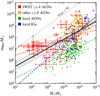 |
Fig. 1 Measurements and fits of the BH mass-stellar mass relation. The data points with errors are from JWST measurements (red; see the appendix) and other high-z measurements (yellow) from I21. The local AGN measurements (green) and the local IG measurements (blue), both from RV15, are shown without errors, but the errors are taken into account in the analysis. The dashed lines show the best fits to each of the datasets separately, and the solid black line shows the best fit combining the high-z data and the local IG data. The grey band shows the scatter in the latter fit. |
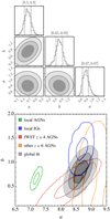 |
Fig. 2 Upper panel: corner plot showing the posteriors for the global fit to JWST (Übler et al. 2023; Larson et al. 2023; Harikane et al. 2023; Bogdan et al. 2024; Ding et al. 2023; Maiolino et al. 2024a; Yue et al. 2023) and previous high-z SMBH data from I21 as well as low-z RV15 data on SMBHs in IGs. Lower panel: 68, 95, and 99.8% CL contours (grey) of the posteriors for a and b defined in Eq. (1), obtained in a global fit that includes all observations except local AGNs by marginalising over σ. For comparison, the 68 and 99.8% CL of individual datasets are shown: JWST high-z measurements (red; Übler et al. 2023; Larson et al. 2023; Harikane et al. 2023; Bogdan et al. 2024; Ding et al. 2023; Maiolino et al. 2024a; Yue et al. 2023), other high-z measurements from I21 (yellow), local IGs (blue), and local AGNs from RV15 (green). The fits were performed using flat priors and including the uncertainties in the observations. Corner plots showing the posterior distributions for these fits are displayed in the appendix. |
3 Analysis of NANOGrav observations
We performed the analysis of the NANOGrav GW signal in the same way as in Ellis et al. (2023, 2024a,b). We summarise here the main features of the model: We related the SMBH merger rate to the halo merger rate, Rh, estimated from the Press-Schechter formalism (Press & Schechter 1974; Bond et al. 1991; Lacey & Cole 1993), as
 (5)
(5)
where pBH characterises the BH merger efficiency and M*(Mv,j, z) is the halo mass-stellar mass relation that we took from Girelli et al. (2020). We included environmental effects parametrised by a spectral index, α, and a reference frequency,
![Mathematical equation: ${t_{{\mathop{\rm int}} }} = {t_{{\rm{GW}}}}{\left[ {{{{f_r}} \over {{f_{{\rm{GW}}}}}}} \right]^\alpha },$](/articles/aa/full_html/2024/11/aa50846-24/aa50846-24-eq8.png) (6)
(6)
where ƒr is the frequency of the emitted GW. The environmental effects drive the binary evolution at frequencies above ƒGW, which we parametrised as ƒGW = fref(ℳ/M⊙)−β. We fixed β = 5/8, corresponding to binary evolution by gas infall (see the discussion below Eq. (12)).
In Ellis et al. (2024a) we found that the local IG fit also gives a much better fit to the NANOGrav GW observations than the local AGN fit, and we now develop this point further. Figure 3 displays in a corner plot the posterior distributions for the parameters of this fit: α, ƒref and pBH. The posterior for α is compatible with models of environmental effects and the fit prefers large values of ƒref ≳ 10 nHz. The preferred range of pBH is [0.16,0.38]. The best fit is achieved at pBH = 0.37, ƒref = 27 nHz and α = 3.3. In particular, the value α = 8/3 expected for gas infall agrees well with the data. By fixing α = 8/3, we find that the best fit is given by pBH = 0.37, ƒref = 30 nHz.
In the upper panel of Fig. 4 we compare our global fit Eq. (3) with the NANOGrav SGWB data (Agazie et al. 2023c) and the best fit SMBH binary GW signals obtained with the BH mass-stellar mass relations derived in P23 and Li et al. (2024). The data and the best-fit simulations are represented by ‘violins’ whose widths represent the posteriors as functions of the GW density: following Ellis et al. (2024a), we calculated the overlaps between the violins to assess the qualities of the fits. For both P23 and Li et al. (2024), the best fits saturate at pBH = 1 (i.e. every galactic merger leads to a GW signal), which is an indication that the generated SGWB is insufficient. Comparing the best-fit likelihoods, we find that the PTA GW background favours the global fit mass relation at higher than the 3σ CL compared to the scaling relations proposed in Pacucci et al. (2023) and Li et al. (2024).
We show in the lower panel of Fig. 4 100 random realisations of the strongest binary contributing to the first NANOGrav bin, ƒGW ∈ (2–4) nHz, for each of the three scenarios. In the case of Li et al. (2024), who advocated for a strong bias in the scaling relation, we can see that the SMBHs are too light, whereas in the case of Pacucci & Loeb (2024), who advocate for a steep z dependence, the heavy SMBH are merging mainly at z > 1, which also decreases the amplitude significantly.
Furthermore, in the lower panel of Fig. 4 we also see that BHs with mBH < 109 M⊙ are very unlikely to be among the strongest sources contributing to the SGWB. Given that the mass and z range probed by NANOGrav coincides with the dynamically measured SMBH masses, the high merger efficiency necessary to explain the observed GW background implies that the local IG population is not significantly biased. The local AGNs lie in a lower mass range, and it is an open question whether that population is biased. However, given the consistency between the high-z AGN measurements and the local IG measurements and the fact that at high z the AGN fraction is close to unity but drops quickly at z ≲ 1 (Aird et al. 2018; Georgakakis et al. 2017), it seems that the local AGN population reflects the intrinsic low-mass tail of the full BH mass-stellar mass relationship.
Comparing the local AGN population to the global fit in Fig. 1 we see that most of the local AGNs lie more than 2σ below the mean of the global fit. Hence, according to this analysis, the AGN fraction in the local SMBH population can only be ≲5%, in agreement with X-ray observations (Aird et al. 2018; Georgakakis et al. 2017). To conclude, in contrast to Li et al. (2024), our analysis indicates that the local AGN population represents the tip of the iceberg of the local SMBH population. As discussed in Ellis et al. (2024a,c), our interpretation of the NANOGrav and JWST data would favour the observability of GW signals from BH binaries in space-borne laser interferometers, for example LISA (Amaro-Seoane et al. 2017), TianQin (Wang et al. 2019), and Taiji (Ruan et al. 2020), and deci-hertz GW detectors, for example AION (Badurina et al. 2020), AEDGE (El-Neaj et al. 2020), and DECIGO (Kawamura et al. 2021).
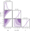 |
Fig. 3 Posterior distributions of the parameters for a fit to NANOGrav GW data (Agazie et al. 2023c) including energy loss due to interactions with the environment. |
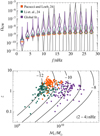 |
Fig. 4 Upper panel: best-fit nanohertz GW signals found using the BH mass-stellar mass relations proposed in Pacucci & Loeb (2024), Li et al. (2024), and our global fit (3) compared to the signal measured by NANOGrav (grey). We imposed α = 8/3, as expected from gas infall (see the discussion below Eq. (12)). Lower panel: chirp masses and red-shifts of 100 realisations of the strongest binary contributing to the first bin of the upper panel for the scenarios proposed in Pacucci & Loeb (2024), and Li et al. (2024) compared with our analysis (Ellis et al. 2024a). Contours of log10ΩGW are shown for comparison. |
4 Dual AGN fraction
We found in Ellis et al. (2024a,c) that the quality of the SMBH fit to the NANOGrav data is improved by allowing for the evolution of the binary system to be affected by interaction with the environment as well as the emission of GWs. A similar conclusion was reached by the NANOGrav Collaboration (Agazie et al. 2023b). We discuss now the extent to which the unexpectedly high fraction of dual AGNs observed with JWST (Perna et al. 2023) can be accommodated within our analysis of high- z SMBH data and NANOGrav SGWB measurements including environmental effects.
We estimated the numbers of dual AGNs and objects that we identified as single AGNs assuming that the collisions of galaxies trigger AGN activity. This is in agreement with numerical simulations (Scudder et al. 2012; Callegari et al. 2011; Capelo et al. 2015) and low-z observations (Treister et al. 2012; Comerford et al. 2015; Donley et al. 2018; Koss et al. 2012), except for a small number of objects (Liu et al. 2018; Mićić et al. 2023). In this way, the AGN observations are linked to the NANOGrav observations and to the BH mass-stellar mass relation through the galaxy merger rate. Environmental effects determine the evolution of the separations of the components in dual systems; therefore, to estimate the numbers of dual AGNs and objects seen as single AGNs, we started by characterising the effective timescales of different environmental effects.
Several such effects are expected to contribute to the binary evolution in different ranges of the binary separation (Kelley et al. 2017), as illustrated in Fig. 5. The effective timescale for the binary evolution is defined as teff ≡ |E|/Ė, where E is the binary total energy. The effective timescale can be expressed as
 (7)
(7)
where tGW is the timescale of the GW driven binary evolution and tenv is the timescale of the environmental effects. For a circular orbit the binary total energy is given by E = −m1m2/d where d denotes the separation of the BHs, so, in terms of the effective timescale, the separation evolves as
 (8)
(8)
The dominant contribution to the binary evolution at small separations arises from GW emission, whose timescale is
![Mathematical equation: ${t_{{\rm{GW}}}} = {{5{d^4}} \over {1024\eta {M^3}}} \approx {{14{\rm{Myr}}} \over \eta }{\left[ {{M \over {{{10}^9}{M_ \odot }}}} \right]^{ - 3}}{\left[ {{d \over {0.1{\rm{pc}}}}} \right]^4},$](/articles/aa/full_html/2024/11/aa50846-24/aa50846-24-eq11.png) (9)
(9)
where η and M denote the symmetric mass ratio and the total mass of the binary. However, other energy-loss mechanisms come into play at separations probed by PTAs and other observations.
At kiloparsec separations, dynamical friction drives the binary evolution (Kelley et al. 2017). Its timescale is (Binney & Tremaine 2008)
![Mathematical equation: ${t_{{\rm{dyn}}}} \simeq {{20{\rm{Myr}}} \over {\ln \Lambda }}{\sigma \over {200{\rm{km/s}}}}{\left[ {{M \over {{{10}^9}{M_ \odot }}}} \right]^{ - 1}}{\left[ {{d \over {{\rm{kpc}}}}} \right]^2},$](/articles/aa/full_html/2024/11/aa50846-24/aa50846-24-eq12.png) (10)
(10)
where ln Λ is the Coulomb logarithm and σ is the velocity dispersion of stars.
Dynamical friction becomes inefficient at shorter distances when the binary binding energy becomes larger than the kinetic energy of the stars whose orbits pass close to the binary. The binary evolution is then driven by loss-cone scattering, whose timescale can be estimated as (Quinlan 1996)
![Mathematical equation: ${t_{{\rm{sh}}}} \simeq {\sigma \over {H\rho d}} \approx 300{\rm{Myr}}{\sigma \over {200{\rm{km/s}}}}{[{\rho \over {10{M_ \odot }/{\rm{p}}{{\rm{c}}^3}}}]^{ - 1}}{[{d \over {{\rm{pc}}}}]^{ - 1}},$](/articles/aa/full_html/2024/11/aa50846-24/aa50846-24-eq13.png) (11)
(11)
where H ≈ 15–20 is the dimensionless hardening rate, and ρ and σ denote the mass density and the velocity dispersion of stars in the neighbourhood of the binary.
At intermediate scales between the GW-driven and loss-cone scattering-driven phases, we used the parametrisation Eq. (6) that is given in terms of the binary separation as
![Mathematical equation: ${t_{{\rm{int}}}} = {t_{{\rm{GW}}}}{\left[ {{d \over {{d_{{\rm{ref}}}}}}} \right]^{ - {{3\alpha } \over 2}}}.$](/articles/aa/full_html/2024/11/aa50846-24/aa50846-24-eq14.png) (12)
(12)
The reference separation dref is related to the reference frequency used in Eq. (6) by  . We estimated the total timescale of the environmental effects as tenv =
  .
.
Effects that potentially determine the dynamics of binaries at intermediate scales include gas infall and viscous drag. The timescale of the binary evolution by gas infall can be estimated from the accretion timescale (Begelman et al. 1980), tgas ≃ m 1/ṁ1, where m1 is the mass of the heavier BH, and the timescale of viscous drag has been estimated in Ivanov et al. (1999) to scale as,  . These correspond, respectively, to (α,β) = (8/3,5/8) and (α,β) ≈ (7/3,3/4), while a transition directly from the loss-cone scattering to GW-driven evolution would correspond to (α,β) = (10/3,2/5). For the PTA fit shown in Fig. 3 we fixed β = 5/8 after checking that the fit is not very sensitive to the value of β. We also find that the above values of α = 8/3 and α = 10/3 provide good fits to the data.
Given the estimates for the effective timescales, we can estimate the expected number of dual and single AGNs detected by JWST. As already noted, we assumed that AGN activity is triggered only during major mergers where the stellar mass of the heavier galaxy is not more than three times the stellar mass of the lighter one. Single AGNs are generated in major mergers in which one of the galaxies did not contain an SMBH. Moreover, dual AGNs are seen as single AGNs if one of the AGNs is not luminous enough or if their angular separation is too small to be resolved.
The expected number of detectable dual AGNs is
 (13)
(13)
where ƒsky is the sky fraction being observed, pdet the probability that the BH is luminous enough to be detectable, and pdual is the probability that a dual AGN is resolvable. Counting all mergers where at least one of the galaxies is occupied by an SMBH that becomes active during the merger and is sufficiently luminous to be detected, the expected number of detectable AGNs is
 (14)
(14)
The merger rate and the evolution of the BH separation enter through
 (15)
(15)
and
 (16)
(16)
where
 (17)
(17)
is the number density of AGNs formed in galaxy mergers where one of the galaxies did not contain an SMBH, and
 (18)
(18)
is the number density of dual AGNs. The probability that a galaxy with stellar mass M* is occupied by an SMBH with mass m can be expressed as
 (19)
(19)
where the distribution dP/dm, given by Eq. (1), is normalised to 1, so  can be interpreted as the SMBH occupation fraction, which we took to be independent of M*. The prefactor
  in Eq. (17) gives the probability that one of the merging galaxies does not contain an SMBH. In this case, dynamical friction drives this single SMBH towards the centre of the galaxy that resulted from the merger. So, for Eq. (17) we estimated the timescale as teff = tdyn. We assumed that the AGN activity starts when the distance between the galaxies becomes smaller than the half-stellar radius of the smaller galaxy. We approximated the half-stellar radius as being 10% of the virial radius of the halo:
 (20)
(20)
In the right panel of Fig. 6 the shades of orange show the dual AGN probability  where dntot is obtained from Eq. (18) with pAGN = 1.
We estimated the detection probability, pdet, by setting a threshold on the flux:
 (21)
(21)
where DL denotes the luminosity distance of the system. We approximated the AGN luminosity optimistically as L ≃ LEdd/3 ≈ 4.3 × 1043 (mBH106M⊙)erg/s and chose Fsens ≃ 10−15 erg/s/cm2, which corresponds to the dimmest source found in Perna et al. (2023). The threshold on the flux gives a redshift-dependent lower bound on the BH mass, as shown in the left panel of Fig. 6.
We estimated the probability, pdual, by assuming that the duality of the AGNs is properly identified if its projected angular separation,
 (22)
(22)
where DA (z) denotes the angular diameter distance of the system and i and ϕ the inclination and phase of the dual, is larger than twice the angular resolution θres ≈ 0.1″ of JWST, and we averaged over the angles i and ϕ:
 (23)
(23)
The probability pdual is shown in the right panel of Fig. 6.
We write the timescales of dynamical friction and stellar loss-cone scattering as tdyn = 20Myr Adyn[M/109M⊙]−1[d/kpc]2 and tsh = 300 Myr Ash[d/pc]−1 (see Eqs. (10) and (11)), and study how the dual AGN fraction  and the total number of
  depend on the parameters Adyn, Ash, pBH, fref and α. We considered the observations reported in Perna et al. (2023) of the GA-NIFS sample of 17 known AGNs at z > 3, of which N1 = 12 were identified as single AGNs, N2 = 4 as dual AGNs and one as a triple AGN. Based on these observations, we estimate that the dual fraction N2 /(N1 + N2) = 0.25. We also considered the JWST results of Kocevski et al. (2024) that cover 587.8 arcmin2, corresponding to fsky ≈ 4 × 10⁻⁶, revealing 341 LRDs in the redshift range 2 < z < 11. Interpreting these LRDs as AGNs, we used this as an observation of the total AGN number, Ntot = 3411.
In the upper panels of Fig. 5 we show the dependences of the numbers of AGNs and fractions of dual AGNs on fref for α = 8/3, corresponding to the gas infall timescale, Ash = 1, Adyn = 0.001 and pBH = 0.2. For these parameters, the lower panel of Fig. 5 illustrates the timescales of the environmental energy loss mechanisms, including GW emission, gas effects, stellar loss-cone scattering and dynamical friction, as functions of the binary separation. The different curves in the lower panel correspond to different values of fref indicated by the coloured dots in the upper panel. The horizontal bands in the upper panel show the 95% CL bands of the JWST LRD and dual AGN observations calculated assuming the Poisson and binomial distribution, respectively. The value of pBH is fixed so that, neglecting AGNs that may form in mergers where only one of the galaxies contains an SMBH, the expected total AGN number roughly matches the LRD observations for large fref. We see in the right panel that, in this benchmark case, the dual fraction is within the 95% range of the observed value for fref > 6 nHz if only the AGNs that may form in mergers where both of the galaxies contain an SMBH are considered. These values of pBH, α and fref are within the 95% CL region of the NANOGrav fit, illustrating that it is possible to obtain a coherent description of the evolution of binary systems that explains both the NANOGrav GW signal and the JWST dual AGN and LRD observations.
Figure 5 shows that the expected number of systems seen as single AGNs would be much larger than observed if fref is small, because in that case, the binaries would spend a lot of time orbiting with d ~ 1 pc separation. This is related to the well-known final-parsec problem. Both the JWST and PTA observations prefer large values of fref for which the final-parsec problem is avoided. Then, the main contribution to the total number of AGNs comes from the same region as for dual AGNs, d ≳ 1 kpc, where the effective timescale is largest. In this regime, both  and
and  are proportional to the prefactor Adyn of the dynamical friction timescale. For the benchmark shown in Fig. 5 we have fixed Adyn = 0.001 so that the result is consistent with the LRD observations for values of pBH consistent with the NANOGrav observations. Larger values of Adyn or pBH than those used in the above benchmark case would increase the total AGN number while the dual fraction would remain roughly the same. Larger values of Ash would instead decrease the dual fraction and increase the total AGN number.
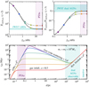 |
Fig. 5 Upper panels: expected total number of AGNs at z > 2 and the expected dual fraction at z > 3 as a function of the reference frequency, below which the binaries are driven by GW emission, assuming pBH = 0.2, α = 8/3, Adyn = 0.001, and Ash = 1. The dashed and solid curves are with and without galaxy mergers and where one of the galaxies does not contain an SMBH. Lower panel: illustration of the timescales of the environmental energy loss mechanisms of SMBH binaries as functions of their separations for the same parameter values as in the upper panels. The vertical bands illustrate the separation ranges probed by the PTAs and by the JWST dual AGN observations. The colour coding of the curves matches that shown in the upper panels. |
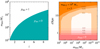 |
Fig. 6 Left panel: detectability probability, pdet, arising from the JWST sensitivity threshold on the flux. Right panel: dual identification probability, pdual, at z = 3 arising from the JWST angular resolution, shown by the red regions. The orange regions show the probability that both galactic nuclei are active for mBH,2 = 108M⊙ at z = 3. |
5 Conclusions
We have presented a global analysis of the available data on high-z SMBHs detected with JWST (Übler et al. 2023; Larson et al. 2023; Harikane et al. 2023; Bogdan et al. 2024; Ding et al. 2023; Maiolino et al. 2024a; Yue et al. 2023) and in previous observations from I21, in conjunction with results from previous samples of SMBHs in low-z AGNs and IGs from RV15 and measurements of the SGWB background by NANOGrav (Agazie et al. 2023c), which are compatible with data from other PTAs (Agazie et al. 2023a). The JWST data are compatible with previous high-z SMBH data, and both are compatible with a sample of low-z IGs but incompatible with a low-z AGN sample (see Fig. 2 and Table 1). Moreover, we have shown that our global fit to the high-z SMBH and local IG data also fits the NANOGrav data on the nanohertz SGWB, whereas alternative interpretations of the high-z SMBH data that evoke an evolution of the MBH/M* relationship evolution with z (Pacucci & Loeb 2024) or selection biases and measurement uncertainties (Li et al. 2024) provide only poor fits to the SGWB data, as seen in Fig. 4.
We have also shown how the dual AGN fraction reported in Perna et al. (2023) can be accommodated within our global analysis. Our interpretation of the data on the dual AGN fraction (Perna et al. 2023) is related to the need for environmental effects to accommodate the spectral shape of the NANOGrav data (see Fig. 3 and the upper panel of Fig. 4 as well as Agazie et al. 2023b and Ellis et al. 2024a). Figure 5 shows that an extrapolation of these environmental effects to larger scales can accommodate the fraction of dual AGNs detected with JWST, can be seen in Fig. 5. Moreover, we also find that our global analysis is compatible with the abundance of LRDs in JWST observations reported recently (Matthee et al. 2024; Kocevski et al. 2024).
Observations of high-z SMBHs are still in their infancy, with much more data to come from JWST and other sources. Likewise, PTA observations of the nanohertz SGWB will develop rapidly in the near future. Doubtless, both sets of data will provide new puzzles. The central point of our paper is that these datasets should be considered together and that these puzzles may share common features. The resolution of these puzzles may also require inputs from other observational programmes, such as measurements of GWs at higher frequencies, interpreted within an integrated approach.
Acknowledgements
This work was supported by the European Regional Development Fund through the CoE program grant TK202 and by the Estonian Research Council grants PRG803, PSG869, RVTT3 and RVTT7. The work of J.E. and M.F. was supported by the United Kingdom STFC Grants ST/T000759/1 and ST/T00679X/1. The work of V.V. was partially supported by the European Union’s Horizon Europe research and innovation program under the Marie Skłodowska-Curie grant agreement No. 101065736.
Appendix A Compilation of JWST data and corner plots
In Fig. A.1 we present corner plots that exhibit the posteriors for the parameters a, b and σ that were introduced in (1) to characterise the BH mass-stellar mass relation for fits to various datasets discussed in the main text. These include the JWST high-z SMBH data compiled in Fig. A.2 (upper left), the previous high-z SMBH data compiled in I21 (upper right), the RV15 data on local AGNs (lower left), and the RV15 data on dynamically measured SMBH (lower right). The latter two fits agree with the fits found by RV15.
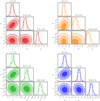 |
Fig. A.1 Posteriors for fits to the JWST high-z SMBH data compiled in Fig. A.2 (upper left), previous high-z SMBH data compiled in I21 (upper right), the RV15 data on local AGNs (lower left), and the RV15 data on the dynamically measured SMBH (lower right). |
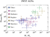 |
Fig. A.2 Scatter plot of the JWST data analysed in this paper. The following are the papers listed in the legend: Übler+ (Übler et al. 2023), Larson+ (Larson et al. 2023), Harikane+ (Harikane et al. 2023), Bogdan+ (Bogdan et al. 2024), Ding+ (Ding et al. 2023), Maiolino+ (Maiolino et al. 2024a), and Yue+ (Yue et al. 2023). |
References
- Agazie, G., Antoniadis, J., Anumarlapudi, A., et al. 2023a, ApJ, submitted [arXiv:2309.00693] [Google Scholar]
- Agazie, G., Anumarlapudi, A., Archibald, A. M., et al. 2023b, ApJ, 952, L37 [NASA ADS] [CrossRef] [Google Scholar]
- Agazie, G., Anumarlapudi, A., Archibald, A. M., et al. 2023c, ApJ, 951, L8 [NASA ADS] [CrossRef] [Google Scholar]
- Aird, J., Coil, A. L., & Georgakakis, A. 2018, MNRAS, 474, 1225 [NASA ADS] [CrossRef] [Google Scholar]
- Akins, H. B., Casey, C. M., Allen, N., et al. 2023, ApJ, 956, 61 [NASA ADS] [CrossRef] [Google Scholar]
- Amaro-Seoane, P., Audley, H., Babak, S., et al. 2017, arXiv e-prints [arXiv:1702.00786] [Google Scholar]
- Ananna, T. T., Bogdán, A., Kovács, O. E., Natarajan, P., & Hickox, R. C. 2024, ApJ, submitted [arXiv:2404.19010] [Google Scholar]
- Antoniadis, J., Arumugam, P., Arumugam, S., et al. 2024, A&A, 685, A94 [NASA ADS] [CrossRef] [EDP Sciences] [Google Scholar]
- Badurina, L., Bentine, E., Blas, D., et al. 2020, JCAP, 05, 011 [CrossRef] [Google Scholar]
- Barro, G., Pérez-González, P. G., Kocevski, D. D., et al. 2024, ApJ, 963, 128 [CrossRef] [Google Scholar]
- Begelman, M. C., Blandford, R. D., & Rees, M. J. 1980, Nature, 287, 307 [Google Scholar]
- Binney, J., & Tremaine, S. 2008, Galactic Dynamics: Second Edition (Princeton: Princeton University Press) [Google Scholar]
- Bogdan, A., Goulding, A. D., Natarajan, P., et al. 2024, Nat. Astron., 8, 126 [Google Scholar]
- Bond, J. R., Cole, S., Efstathiou, G., & Kaiser, N. 1991, ApJ, 379, 440 [NASA ADS] [CrossRef] [Google Scholar]
- Callegari, S., Kazantzidis, S., Mayer, L., et al. 2011, ApJ, 729, 85 [NASA ADS] [CrossRef] [Google Scholar]
- Capelo, P. R., Volonteri, M., Dotti, M., et al. 2015, MNRAS, 447, 2123 [NASA ADS] [CrossRef] [Google Scholar]
- Comerford, J. M., Pooley, D., Barrows, R. S., et al. 2015, ApJ, 806, 219 [Google Scholar]
- Ding, X., Onoue, M., Silverman, J. D., et al. 2023, Nature, 621, 51 [NASA ADS] [CrossRef] [Google Scholar]
- Donley, J. L., Kartaltepe, J., Kocevski, D., et al. 2018, ApJ, 853, 63 [NASA ADS] [CrossRef] [Google Scholar]
- Ellis, J., Fairbairn, M., Hütsi, G., et al. 2023, A&A, 676, A38 [NASA ADS] [CrossRef] [EDP Sciences] [Google Scholar]
- Ellis, J., Fairbairn, M., Hütsi, G., et al. 2024a, Phys. Rev. D, 109, L021302 [NASA ADS] [CrossRef] [Google Scholar]
- Ellis, J., Fairbairn, M., Urrutia, J., & Vaskonen, V. 2024b, ApJ, 964, 11 [NASA ADS] [CrossRef] [Google Scholar]
- Ellis, J., Fairbairn, M., Franciolini, G., et al. 2024c, Phys. Rev. D, 109, 023522 [NASA ADS] [CrossRef] [Google Scholar]
- El-Neaj, Y. A., Alpigiani, C., Amairi-Pyka, S., et al. 2020, EPJ Quant. Technol., 7, 6 [CrossRef] [Google Scholar]
- Georgakakis, A., Aird, J., Schulze, A., et al. 2017, MNRAS, 471, 1976 [NASA ADS] [CrossRef] [Google Scholar]
- Girelli, G., Pozzetti, L., Bolzonella, M., et al. 2020, A&A, 634, A135 [NASA ADS] [CrossRef] [EDP Sciences] [Google Scholar]
- Harikane, Y., Zhang, Y., Nakajima, K., et al. 2023, ApJ, 959, 39 [NASA ADS] [CrossRef] [Google Scholar]
- Ivanov, P. B., Papaloizou, J. C. B., & Polnarev, A. G. 1999, MNRAS, 307, 79 [Google Scholar]
- Izumi, T., Matsuoka, Y., Fujimoto, S., et al. 2021, ApJ, 914, 36 [CrossRef] [Google Scholar]
- Kawamura, S., Ando, M., Seto, N., et al. 2021, Prog. Theor. Exp. Phys., 2021, 05A105 [CrossRef] [Google Scholar]
- Kelley, L. Z., Blecha, L., & Hernquist, L. 2017, MNRAS, 464, 3131 [NASA ADS] [CrossRef] [Google Scholar]
- Kocevski, D. D., Finkelstein, S. L., Barro, G., et al. 2024, arXiv e-prints [arXiv:2404.03576] [Google Scholar]
- Koss, M., Mushotzky, R., Treister, E., et al. 2012, ApJ, 746, L22 [Google Scholar]
- Labbé, I., Greene, J. E., Bezanson, R., et al. 2023a, arXiv e-prints [arXiv:2306.07320] [Google Scholar]
- Labbé, I., van Dokkum, P., Nelson, E., et al. 2023b, Nature, 616, 266 [CrossRef] [Google Scholar]
- Lacey, C. G., & Cole, S. 1993, MNRAS, 262, 627 [NASA ADS] [CrossRef] [Google Scholar]
- Larson, R. L., Finkelstein, S. L., Kocevski, D. D., et al. 2023, ApJ, 953, L29 [NASA ADS] [CrossRef] [Google Scholar]
- Li, J., Silverman, J. D., Shen, Y., et al. 2024, arXiv e-prints [arXiv:2403.00074] [Google Scholar]
- Liu, X., Guo, H., Shen, Y., Greene, J. E., & Strauss, M. A. 2018, ApJ, 862, 29 [NASA ADS] [CrossRef] [Google Scholar]
- Maiolino, R., Scholtz, J., Curtis-Lake, E., et al. 2024a, A&A, 691, A145 [NASA ADS] [CrossRef] [EDP Sciences] [Google Scholar]
- Maiolino, R., Risaliti, G., Signorini, M., et al. 2024b, arXiv e-prints [arXiv:2405.00504] [Google Scholar]
- Matthee, J., Naidu, R. P., Brammer, G., et al. 2024, ApJ, 963, 129 [NASA ADS] [CrossRef] [Google Scholar]
- Mićić, M., Wells, B. N., Holmes, O. J., & Irwin, J. A. 2023, arXiv e-prints [arXiv:2310.09945] [Google Scholar]
- Pacucci, F., & Loeb, A. 2024, arXiv e-prints [arXiv:2401.04159] [Google Scholar]
- Pacucci, F., Nguyen, B., Carniani, S., Maiolino, R., & Fan, X. 2023, arXiv e-prints [arXiv:2308.12331] [Google Scholar]
- Padmanabhan, H., & Loeb, A. 2024, A&A, 684, L15 [NASA ADS] [CrossRef] [EDP Sciences] [Google Scholar]
- Perna, M., Arribas, S., Lamperti, I., et al. 2023, arXiv e-prints [arXiv:2310.03067] [Google Scholar]
- Press, W. H., & Schechter, P. 1974, ApJ, 187, 425 [Google Scholar]
- Quinlan, G. D. 1996, New Astron., 1, 35 [Google Scholar]
- Reardon, D. J., Zic, A., Shannon, R. M., et al. 2023, ApJ, 951, L6 [NASA ADS] [CrossRef] [Google Scholar]
- Reines, A. E., & Volonteri, M. 2015, ApJ, 813, 82 [NASA ADS] [CrossRef] [Google Scholar]
- Ruan, W.-H., Guo, Z.-K., Cai, R.-G., & Zhang, Y.-Z. 2020, Int. J. Mod. Phys. A, 35, 2050075 [NASA ADS] [CrossRef] [Google Scholar]
- Scudder, J. M., Ellison, S. L., Torrey, P., Patton, D. R., & Mendel, J. T. 2012, MNRAS, 426, 549 [NASA ADS] [CrossRef] [Google Scholar]
- Treister, E., Schawinski, K., Urry, C. M., & Simmons, B. D. 2012, ApJ, 758, L39 [NASA ADS] [CrossRef] [Google Scholar]
- Übler, H., Maiolino, R., Curtis-Lake, E., et al. 2023, A&A, 677, A145 [NASA ADS] [CrossRef] [EDP Sciences] [Google Scholar]
- Wang, H.-T., Jiang, Z., Sesana, A., et al. 2019, Phys. Rev. D, 100, 043003 [NASA ADS] [CrossRef] [Google Scholar]
- Xu, H., Chen, S., Guo, Y., et al. 2023, arXiv e-prints [arXiv:2306.16216] [Google Scholar]
- Yue, M., Eilers, A.-C., Simcoe, R. A., et al. 2023, arXiv e-prints [arXiv:2309.04614] [Google Scholar]
The origin of the LRDs is debated because they are not detected in X-rays (Ananna et al. 2024). However, the non-detection of X-rays may be caused by high obscuration or intrinsic X-ray weakness of the AGNs (Maiolino et al. 2024b). Our objective is to determine whether the surprisingly high number density of LRDs can be accounted for under the assumption that they are AGNs whose nuclear activity is triggered during mergers. Determining, whether this mechanism could be responsible for triggering local AGN activity, exceeds the scope of this letter and is left for future work.
All Tables
All Figures
|
Fig. 1 Measurements and fits of the BH mass-stellar mass relation. The data points with errors are from JWST measurements (red; see the appendix) and other high-z measurements (yellow) from I21. The local AGN measurements (green) and the local IG measurements (blue), both from RV15, are shown without errors, but the errors are taken into account in the analysis. The dashed lines show the best fits to each of the datasets separately, and the solid black line shows the best fit combining the high-z data and the local IG data. The grey band shows the scatter in the latter fit. |
| In the text | |
|
Fig. 2 Upper panel: corner plot showing the posteriors for the global fit to JWST (Übler et al. 2023; Larson et al. 2023; Harikane et al. 2023; Bogdan et al. 2024; Ding et al. 2023; Maiolino et al. 2024a; Yue et al. 2023) and previous high-z SMBH data from I21 as well as low-z RV15 data on SMBHs in IGs. Lower panel: 68, 95, and 99.8% CL contours (grey) of the posteriors for a and b defined in Eq. (1), obtained in a global fit that includes all observations except local AGNs by marginalising over σ. For comparison, the 68 and 99.8% CL of individual datasets are shown: JWST high-z measurements (red; Übler et al. 2023; Larson et al. 2023; Harikane et al. 2023; Bogdan et al. 2024; Ding et al. 2023; Maiolino et al. 2024a; Yue et al. 2023), other high-z measurements from I21 (yellow), local IGs (blue), and local AGNs from RV15 (green). The fits were performed using flat priors and including the uncertainties in the observations. Corner plots showing the posterior distributions for these fits are displayed in the appendix. |
| In the text | |
|
Fig. 3 Posterior distributions of the parameters for a fit to NANOGrav GW data (Agazie et al. 2023c) including energy loss due to interactions with the environment. |
| In the text | |
|
Fig. 4 Upper panel: best-fit nanohertz GW signals found using the BH mass-stellar mass relations proposed in Pacucci & Loeb (2024), Li et al. (2024), and our global fit (3) compared to the signal measured by NANOGrav (grey). We imposed α = 8/3, as expected from gas infall (see the discussion below Eq. (12)). Lower panel: chirp masses and red-shifts of 100 realisations of the strongest binary contributing to the first bin of the upper panel for the scenarios proposed in Pacucci & Loeb (2024), and Li et al. (2024) compared with our analysis (Ellis et al. 2024a). Contours of log10ΩGW are shown for comparison. |
| In the text | |
|
Fig. 5 Upper panels: expected total number of AGNs at z > 2 and the expected dual fraction at z > 3 as a function of the reference frequency, below which the binaries are driven by GW emission, assuming pBH = 0.2, α = 8/3, Adyn = 0.001, and Ash = 1. The dashed and solid curves are with and without galaxy mergers and where one of the galaxies does not contain an SMBH. Lower panel: illustration of the timescales of the environmental energy loss mechanisms of SMBH binaries as functions of their separations for the same parameter values as in the upper panels. The vertical bands illustrate the separation ranges probed by the PTAs and by the JWST dual AGN observations. The colour coding of the curves matches that shown in the upper panels. |
| In the text | |
|
Fig. 6 Left panel: detectability probability, pdet, arising from the JWST sensitivity threshold on the flux. Right panel: dual identification probability, pdual, at z = 3 arising from the JWST angular resolution, shown by the red regions. The orange regions show the probability that both galactic nuclei are active for mBH,2 = 108M⊙ at z = 3. |
| In the text | |
|
Fig. A.1 Posteriors for fits to the JWST high-z SMBH data compiled in Fig. A.2 (upper left), previous high-z SMBH data compiled in I21 (upper right), the RV15 data on local AGNs (lower left), and the RV15 data on the dynamically measured SMBH (lower right). |
| In the text | |
|
Fig. A.2 Scatter plot of the JWST data analysed in this paper. The following are the papers listed in the legend: Übler+ (Übler et al. 2023), Larson+ (Larson et al. 2023), Harikane+ (Harikane et al. 2023), Bogdan+ (Bogdan et al. 2024), Ding+ (Ding et al. 2023), Maiolino+ (Maiolino et al. 2024a), and Yue+ (Yue et al. 2023). |
| In the text | |
Current usage metrics show cumulative count of Article Views (full-text article views including HTML views, PDF and ePub downloads, according to the available data) and Abstracts Views on Vision4Press platform.
Data correspond to usage on the plateform after 2015. The current usage metrics is available 48-96 hours after online publication and is updated daily on week days.
Initial download of the metrics may take a while.