© The Authors 2024

1 Introduction

The pulsar timing array (PTA) collaborations have recently found compelling evidence for the Hellings-Down quadrupo- lar correlation (Hellings & Downs 1983) within the previously observed common-spectrum stochastic process (Agazie et al. 2023a; Antoniadis et al. 2023b,a; Reardon et al. 2023a; Zic et al. 2023; Reardon et al. 2023b; Xu et al. 2023). This indicates that the observed signal likely originates from a stochastic background of gravitational waves (GWs), the measurement of which marks a significant milestone in GW astronomy. Such a GW background at nHz frequencies can be naturally sourced by a population of inspiraling supermassive black hole (SMBH) binaries (Agazie et al. 2023b; Antoniadis et al. 2024; Ellis et al. 2024b,a).

The naive expectation of the GW background from circular SMBH binaries, a power-law with a spectral index of 13/3 (Phinney 2001), does not provide a good fit to the data, and less steep spectra are preferred. The fit improves significantly once the stochastic nature of the background and energy loss via environmental effects are included (Ellis et al. 2024b). The additional energy loss also aids in solving the final parsec problem (Begelman et al. 1980), as the energy loss shortens the timescale of tightly bound binary formation to reasonable (sub-Hubble time) lengths (Ellis et al. 2024c).

The SMBH binaries are formed in mergers of galaxies (Begelman et al. 1980) and typically have very high initial eccentricities (Fastidio et al. 2024). Whether the binary retains its high initial eccentricity when it reaches parsec separations, where the emission of GWs becomes relevant, is unclear and has been studied with simulations and semi-analytic models (Dotti et al. 2007; Miranda et al. 2017; D’Orazio & Duffell 2021; Berczik et al. 2006; Vasiliev et al. 2015; Gualandris et al. 2022; Kelley et al. 2017; Fastidio et al. 2024).

If the binary is in a gas-rich environment and forms a circumbinary disk, the eccentricity of the binary evolves by interactions with the gas. For circular circumbinary disks, it is expected that, at the pericenter, the SMBH orbits faster than the disk and the disk tends to slow it down. In contrast, at the apocenter, the SMBH orbits slower than the disk and the disk tends to speed it up. This circularizes the binary making the SMBH coalesce with a negligible eccentricity (Dotti et al. 2007). However, more recent simulations suggest that angular momentum transfer between the binary and the accretion disk could maintain large eccentricities and increase the separation (Miranda et al. 2017). A transition between the circular and the precessing disk has been found to happen at around e ~ 0.4 (D’Orazio & Duffell 2021; Zrake et al. 2021), and all initial eccentricities e ≳ 𝒪(0.1) end up at e ~ 0.4 while for e ≲ 𝒪(0.1) the circumbinary disk remains circular and circularizes the orbits.

On the other hand, if the merger happens in a gas-poor environment, loss-cone scattering can drive the binary to sub-parsec separation in a sub-Hubble time if the loss-cone is refilled sufficiently fast (Berczik et al. 2006; Vasiliev et al. 2015). The loss-cone scattering phase is stochastic and its overall effect on the eccentricity distribution depends on the number of stellar encounters (Nasim et al. 2020; Rawlings et al. 2023), on the initial eccentricity (Gualandris et al. 2022), on the geometry of the stellar background (Rawlings et al. 2023) and the mass ratio of the SMBH binary (Gualandris et al. 2022). Overall, these effects can circularize the orbit or, for comparable mass binaries, preserve the high eccentricity. During hardening, eccentricity might increase in minor mergers but is reduced in major ones, permitting large eccentricities of up to e ~ 0.8 (Gualandris et al. 2022) at the onset of the GW-driven phase. Furthermore, the results of the Illustris simulation indicate that SMBH binaries can preserve a very high eccentricity up to the point they enter the PTA band (Kelley et al. 2017; Fastidio et al. 2024).

Although a clear consensus is lacking about the eccentricity distribution of SMBH binaries entering the PTA frequency band, it is possible that their eccentricities can be relatively high. Thus, in light of the recent PTA data, it is not only important to understand how the eccentricity would affect the nHz GW spectrum from SMBHs, but a good theoretical picture of the latter will assist us in resolving the properties of the SMBH binary population.

In this paper, we studied how eccentricities of SMBH binaries affect the nHz GW background. Large eccentricities in the GW-dominated stage of binary evolution lead to a suppression of the GW signal, due to faster orbital decay (Enoki & Nagashima 2007; Sesana 2013; Huerta et al. 2015; Chen et al. 2017; Bi et al. 2023). Since GW-emission circularizes the orbits, this effect is more relevant at lower frequencies where larger average eccentricities are expected. We showed that the eccentricity-induced suppression improves the fit to the NANOGrav 15-year (NG15) data (Agazie et al. 2023a). Furthermore, we found that the effect of eccentricity on the GW background was remarkably similar to that expected from environmental effects (Ellis et al. 2024b).

2 GW emission of eccentric SMBHs

Unlike circular binaries, eccentric binaries emit GWs at multiple frequencies. A binary with a given orbital frequency, f_b , emits GWs at the rest frame frequencies $$f_{n,\text{r}}=(1+z)f_n=n{f}_{\text{b}},$$(1)

where n ≥ 1 is the harmonic number and f_n is the measured GW frequency of the nth harmonic. For circular binaries, only the n = 2 harmonic is present. An eccentric SMBH binary emits GWs in the nth harmonic with power (Peters & Mathews 1963)¹ $$\begin{array}{l}\frac{\text{d}{E}_n}{\hspace{0.17em}\text{d}{t}_r}=\frac{32}{5}{\left(2\pi ℳf_{\text{b}}\right)}^{10/3}{g}_n(e)\\ =\frac{\text{d}{E}_c}{\hspace{0.17em}\text{d}{t}_r}{g}_n(e),\end{array}$$(2)

where 𝓜 denotes the chirp mass and dE_c/dt_r is the power emitted by a circular binary with the same binary parameters 𝓜, f_b and z. The observed time t is related to the time t_r in the rest frame of the binary by dt = (1 + z)dt_r. The relative power radiated in the nth harmonic is $$\begin{array}{ll}{g}_n(e)=\hfill & \frac{n^4}{32}[\frac{4}{3n^2}{J}_n^2(ne)+(J_{n-2}(ne)-2e{J}_{n-1}(ne)\hfill \\ & {+\frac{2}{n}{J}_n(ne)+2e{J}_{n+1}(ne)-J_{n+2}(ne))}^2\hfill \\ \hfill & +\left(1-e^2\right){\left(J_{n-2}(ne)-2J_n(ne)+J_{n+2}(ne)\right)}^2],\end{array}$$(3)

where J_n is the nth Bessel function of the first kind. For circular binaries, only the second harmonic contributes g_n(0) = δ_2n. The total power emitted by a binary across all frequencies is $$\frac{\text{d}{E}_{\text{GW}}}{\hspace{0.17em}\text{d}{t}_r}=\frac{\text{d}{E}_c}{\hspace{0.17em}\text{d}{t}_r}ℱ(e),$$(4)

where $$ℱ(e)={\displaystyle \sum _{n=1}^{\infty }{g}_n}(e)=\frac{1+73/24e^2+37/96e^4}{{\left(1-e^2\right)}^{7/2}}.$$(5)

GW emission by an eccentric binary, e > 0, is enhanced compared to emission by a circular binary by 𝓕(e) > 1.

The increase in the total emitted GW power does not necessarily lead to an increase in the GW background because the increase in the emitted power accelerates the orbital decay of the binary. The orbital dynamics of an eccentric binary are described by the evolution of its orbital frequency and eccentricity (Peters & Mathews 1963) $$\begin{array}{l}\frac{\text{d}\hspace{0.17em}\ln f_{\text{b}}}{\hspace{0.17em}\text{d}{t}_r}=\frac{96}{5}{ℳ}^{5/3}{\left(2\pi f_{\text{b}}\right)}^{8/3}ℱ(e),\\ \frac{\text{d}e}{\hspace{0.17em}\text{d}{t}_r}=-\frac{1}{15}{ℳ}^{5/3}{\left(2\pi f_{\text{b}}\right)}^{8/3}\mathcal{G}(e),\end{array}$$(6)

where $$\mathcal{G}(e)=\frac{304e+121e^3}{{\left(1-e^2\right)}^{5/2}}.$$(7)

From this, the observed residence time of a binary at orbital frequency f_b is $$\begin{array}{l}\frac{\text{d}t}{\hspace{0.17em}\text{d}\hspace{0.17em}\ln f_{\text{b}}}=\frac{5}{96}\frac{1+z}{{ℳ}^{5/3}}{\left(2\pi f_{\text{b}}\right)}^{-8/3}\frac{1}{ℱ(e)}\\ =\frac{\text{d}{t}_c}{\hspace{0.17em}\text{d}\hspace{0.17em}\ln f_{\text{b}}}\frac{1}{ℱ(e)},\end{array}$$(8)

where dt_c/d ln f_b is the observed residence time of the corresponding circular binary (i.e., at e = 0) and the factor 1 + z arises from the conversion of the binary rest frame time t_r to the time t in the observer frame.

3 Eccentricity distribution

The orbital evolution of the SMBH binaries is very slow compared to the PTA observation times, so the binaries can be treated as having a constant orbital frequency and eccentricity from an observational point of view. On the other hand, Eq. (6) gives $$\frac{\text{d}e}{\hspace{0.17em}\text{d}\hspace{0.17em}\ln f_{\text{b}}}=-\frac{1}{288}\frac{\mathcal{G}(e)}{ℱ(e)},$$(9)

indicating a strong relation between the eccentricity of a binary and its frequency. Binaries with higher orbital frequencies are more likely to have lower eccentricities because the GW emission circularizes their orbits. By (9), eccentricity evolution in a GW-driven regime can be described by $$f_{\text{b}}\propto {\left(1-e^2\right)}^{\frac{3}{2}}{e}^{-\frac{18}{19}}{\left(304+121e^2\right)}^{-\frac{1305}{2295}}.$$(10)

Importantly, it is universal, that is, it does not depend on binary masses, if there are no additional environmental effects.

We started with fixing the initial eccentricity distribution, P(e, f₀) = P₀(e) at some initial orbital frequency f₀ (see also Huerta et al. 2015 and Chen et al. 2017). Eq. (10) gives the evolution of eccentricity with frequency, $e=\tilde{e}\left(e_0,f_{\text{b}}/f_0\right)$. This can be inverted to give $e_0=\tilde{e}\left(e,f_0/f_{\text{b}}\right)$ and, since probability is conserved, the distribution of eccentricities at frequency f is $$P\left(e\mid f_{\text{b}}\right)=\frac{\text{d}\tilde{e}\left(e,f_0/f_{\text{b}}\right)}{\text{d}e}{P}_0\left(\tilde{e}\left(e,f_0/f_{\text{b}}\right)\right).$$(11)

For the initial distribution, we consider a power law, $$P_0(e)=(\gamma +1)e^{\gamma },$$(12)

with γ > −1. Although it is a generic phenomenological ansatz, it has some physical motivation as, for instance, γ = 1 corresponds to the “thermal” distribution (Jeans 1919). In the following, we characterized the distribution using the mean initial eccentricity, which is related to the parameter γ as $${\langle e\rangle }_{f_0}=\frac{1+\gamma }{2+\gamma },$$(13)

or inversely, γ = −(1 − 2〈e〉f₀)/(1 − 〈e〉f₀). An example of how the evolution of eccentricity affects its distribution at different frequencies is shown in Fig. 1 for a uniform initial distribution (γ = 0).

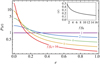Fig. 1 Evolution of an eccentricity distribution set to be uniform at f = f0. The inset shows the evolution of the expectation value of e.

4 Mean GW spectrum

The mean GW spectrum generated by eccentric SMBH binaries is $$\begin{array}{l}\langle \mathrm{\Omega }(f)\rangle =\frac{1}{{\rho }_c}{\displaystyle \int \hspace{0.17em}\text{d}}\lambda \hspace{0.17em}\text{d}e\hspace{0.17em}\text{d}{f}_{\text{b}}{\displaystyle \sum _{n=1}^{\infty }\delta }\left(f_{\text{b}}-\frac{f_{\text{r}}}{n}\right)\\ \times P\left(e\mid f_{\text{b}}\right)\frac{1+z}{4\pi D_L^2}\frac{\hspace{0.17em}\text{d}{E}_n}{\hspace{0.17em}\text{d\hspace{0.17em}}\ln f_{\text{b}}},\end{array}$$(14)

where ρ_c is the critical energy density, D_L is the source luminosity distance and the delta function picks binaries whose nth harmonic contributes to the observed frequency f = f_r/(1 + z). The differential merger rate of BHs in the observer reference frame is $$\text{d}\lambda =\text{d}ℳ\hspace{0.17em}\text{d}\eta \hspace{0.17em}\text{d}z\frac{1}{1+z}\frac{\hspace{0.17em}\text{d}{V}_c}{\hspace{0.17em}\text{d}z}\frac{\hspace{0.17em}\text{d}{R}_{\text{BH}}}{\hspace{0.17em}\text{d}ℳd\eta },$$(15)

where η is the symmetric mass ratio, V_c the comoving volume, and R_BH the comoving BH merger rate density.

Following Ellis et al. (2024b), we used the halo merger rate R_h arising from the extended Press-Schechter formalism (Press & Schechter 1974; Bond et al. 1991; Lacey & Cole 1993)², and converted it to the BH merger rate through a halo mass-BH mass relation $$\begin{array}{l}\frac{\text{d}{R}_{\text{BH}}}{\hspace{0.17em}\text{d}{m}_1\hspace{0.17em}\text{d}{m}_2}=p_{\text{BH}}{\displaystyle \int \hspace{0.17em}\text{d}}{M}_{\text{v},1}\hspace{0.17em}\text{d}{M}_{\text{v},2}\frac{\hspace{0.17em}\text{d}{R}_h}{\hspace{0.17em}\text{d}{M}_{\text{v},1}\hspace{0.17em}\text{d}{M}_{\text{v},2}}\\ \times {\displaystyle \prod _{j=1,2}\frac{\hspace{0.17em}\text{d}P\left(m_j\mid M_{*}\left(M_{\text{v},j},z\right)\right)}{\text{d}{m}_j}},\end{array}$$(16)

where m_j are the masses of the merging BHs, M_v,j are the virial masses of their host halos and p_BH ≤ 1 combines the SMBH occupation fraction in galaxies with the efficiency for the BHs to merge following the merging of their host halos. Due to the GW background being generated by binaries with a narrow range of SMBH masses and redshifts, p_BH was treated as a constant free parameter. We estimated the mass relation using the observed halo mass-stellar mass relation M_*(M_v,j, z) from Girelli et al. (2020) and the global fit stellar mass-BH mass relation from Ellis et al. (2024c). The latter is given by $$\frac{\text{d\hspace{0.17em}}P\left(m\mid M_{\ast }\right)}{\text{d\hspace{0.17em}}{\log }_{10}m}=\mathcal{N}\left({\log }_{10}\frac{m}{M_{\odot }}|a+b{\log }_{10}\frac{M_{\ast }}{{10}^{11}{M}_{\odot }},\sigma \right),$$(17)

with a = 8.6, b = 0.8 and σ = 0.8, where $\mathcal{N}(x\mid \overline{x},\sigma )$ denotes the probability density of a Gaussian distribution with mean $\overline{x}$ and variance σ². We assume that eccentricity does not significantly affect the merger rate.

The residence time at each emitting frequency is reduced for eccentric binaries, leading to an energy emitted per logarithmic frequency interval of $$\frac{\text{d}{E}_n}{\hspace{0.17em}\text{d}\hspace{0.17em}\ln f_{\text{b}}}=\frac{\text{d}{t}_c}{\hspace{0.17em}\text{d}\hspace{0.17em}\ln f_{\text{b}}}\frac{1}{1+z}\frac{\hspace{0.17em}\text{d}{E}_c}{\hspace{0.17em}\text{d}{t}_r}\frac{g_n(e)}{ℱ(e)}.$$(18)

Now, using (18), the mean GW abundance (14) can be expressed as $$\begin{array}{l}\langle \mathrm{\Omega }(f)\rangle ={{\displaystyle \int \text{d}}\lambda \hspace{0.17em}\text{d}e{\displaystyle \sum _{n=1}^{\infty }P}\left(e\mid f_{\text{b}}\right)\frac{g_n(e)}{ℱ(e)}{\mathrm{\Omega }}_c^{(1)}\frac{\text{d}{t}_c}{\hspace{0.17em}\text{d\hspace{0.17em}}\ln f_{\text{b}}}|}_{f_{\text{b}}=\frac{f_{\text{r}}}{n}}\\ ={{\displaystyle \int \text{d}}\lambda ℰ\left(f_{\text{r}}\right){\mathrm{\Omega }}_c^{(1)}\frac{\text{d}{t}_c}{\hspace{0.17em}\text{d\hspace{0.17em}}\ln f_{\text{b}}}|}_{f_{\text{b}}=\frac{f_{\text{r}}}{2}},\end{array}$$(19)

where we defined $${\mathrm{\Omega }}_c^{(1)}\equiv \frac{1}{4\pi D_L^2{\rho }_c}\frac{\hspace{0.17em}\text{d}{E}_c}{\hspace{0.17em}\text{d}{t}_r}$$(20)

denoting the contribution from a single circular binary, and³ $$ℰ\left(f_{\text{r}}\right)\equiv {\displaystyle \sum _{n=1}^{\infty }{\left[\frac{2}{n}\right]}^{2/3}}{\displaystyle \int \hspace{0.17em}\text{d}}eP\left(e\mid f_{\text{r}}/n\right)\frac{g_n(e)}{ℱ(e)}.$$(21)

which quantifies how non-zero eccentricities modify the mean GW spectrum of circular binaries. For circular binaries, P(e) = δ(e) and ℰ(f_r) = 1. Eq. (21) agrees with Huerta et al. (2015, Eq. (36)) for delta distributions P(e) = δ(e − e₀). We remarked that the second line of (19) holds only for inspiraling binaries when the binary evolution is driven purely by GW emission and environmental effects can be neglected.

From the initial eccentricity distribution and its evolution, we evaluated (21) which shows how eccentricity affects the mean GW spectrum. In Fig. 2, we showed ℰ( f ) for different initial eccentricity distributions. Since GW emission circularizes orbits as the orbital frequency increases, ℰ( f ) reaches unity at f ≫ f₀ . High initial eccentricities suppress the spectrum at low frequencies. For a power-law P₀(e) we find that ℰ( f ) increases monotonously with f whereas for P₀(e) = δ(e − e₀) (or for narrow peaked distributions), it increases until it gets mildly larger and starts to approach unity from above.

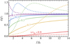Fig. 2 Function E defined in (21) that describes the modification of the mean GW spectrum caused by the binary eccentricities shown for power-law (solid) and delta function (dashed) initial eccentricity distributions and different values of mean eccentricity of the initial distribution fixed at f = f0.

5 Statistics of GW spectra

Given that the binary separation and the eccentricity evolve slowly when compared to an orbital period, the observed GW spectrum of a single binary can be expressed as a sum of individual harmonics: $${\mathrm{\Omega }}^{(1)}(f)={\mathrm{\Omega }}_c^{(1)}{\displaystyle \sum _{n\ge 1}{g}_n}(e)f\delta \left(f-\frac{n}{2}{f}_2\right).$$(22)

Thus, the statistical properties of the GW spectrum of SMBH binaries can be inferred from the distribution of Ω_c and e (or an equivalent set of parameters) at a given f₂ (or observed orbital frequency f₁ ) and the number of SMBH binaries in a given range of f₂ . In the following, we considered the distribution $$\begin{array}{l}{P}^{(1)}\left({\mathrm{\Omega }}_c,e\mid f_2\right)={\left(\frac{\text{d}N}{\hspace{0.17em}\text{d}\hspace{0.17em}\ln f_2}\right)}^{-1}{\displaystyle \int \hspace{0.17em}\text{d}}\lambda P\left(e\mid f_{\text{b}}\right)\\ \times {\frac{\text{d}{t}_c}{\hspace{0.17em}\text{d}\hspace{0.17em}\ln f_{\text{b}}}\delta \left({\mathrm{\Omega }}_c-{\mathrm{\Omega }}_c^{(1)}\right)|}_{f_b=\frac{f_{2,r}}{2}},\end{array}$$(23)

where the number of SMBHs per a logarithmic f₂ interval is $$\frac{\text{d}N}{\hspace{0.17em}\text{d\hspace{0.17em}}\ln f_2}={{\displaystyle \int \text{d}}\lambda \frac{\hspace{0.17em}\text{d}{t}_c}{\hspace{0.17em}\text{d\hspace{0.17em}}\ln f_{\text{b}}}|}_{f_{\text{b}}=\frac{f_{2,r}}{2}}.$$(24)

The mean (19) is recovered as $$\begin{array}{l}\langle \mathrm{\Omega }(f)\rangle ={\displaystyle \int \text{d}}e\hspace{0.17em}\text{d}{\mathrm{\Omega }}_c{\displaystyle \sum _n\frac{{\mathrm{\Omega }}_c{g}_n(e)}{ℱ(e)}}\\ \times {\frac{\text{d}N}{\hspace{0.17em}\text{d\hspace{0.17em}}\ln f_2}{P}^{(1)}\left({\mathrm{\Omega }}_c,e\mid f_2\right)|}_{f_2=\frac{2f}{n}}.\end{array}$$(25)

Higher order correlation functions can be computed similarly from P⁽¹⁾(Ω_c, e|f_շ).

5.1 Distribution at a frequency

The GW spectrum in a given frequency bin f_j can be computed by integrating over eccentricities e. The distribution of Ω_c and e at a given f₂ can then be converted into a distribution of contributions Ω from individual binaries at a given frequency f, $$\begin{array}{l}{P}^{(1)}(\mathrm{\Omega }\mid f)={\left(\frac{\text{d}N}{\hspace{0.17em}\text{d\hspace{0.17em}}\ln f}\right)}^{-1}{\displaystyle \int \hspace{0.17em}\text{d}}e\hspace{0.17em}\text{d}\lambda {\displaystyle \sum _{n=1}^{\infty }\frac{P\left(e\mid f_{\text{b}}\right)}{ℱ(e)}}\\ \times {\frac{\text{d}{t}_c}{\hspace{0.17em}\text{d\hspace{0.17em}}\ln f_{\text{b}}}\delta \left(\mathrm{\Omega }-{\mathrm{\Omega }}_c^{(1)}{g}_n(e)\right)|}_{f_{\text{b}}=\frac{f_r}{n}},\end{array}$$(26)

where $$\frac{\text{d}N}{\hspace{0.17em}\text{d\hspace{0.17em}}\ln f}={{\displaystyle \int \text{d}}\lambda \frac{\hspace{0.17em}\text{d}{t}_c}{\hspace{0.17em}\text{d\hspace{0.17em}}\ln f_{\text{b}}}|}_{f_b=\frac{f_r}{2}}.$$(27)

The only difference with the approach developed in Ellis et al. (2023) and Ellis et al. (2024b) is that now the expression includes a sum over the harmonics n, an integral over eccentricity e, with the appropriate g_n(e) and 𝓕(e) factors, and the distribution of eccentricities. Consequently, the derivation of the statistical properties of the GW spectrum presented below has a sizeable overlap with these references.

We computed the distribution of the total GW abundance in frequency bins, P(Ω| f_j), by dividing the sources into strong sources, above some threshold Ω > Ω_thr, and weak sources, Ω < Ω_thr. The strong sources were modelled via Monte-Carlo (MC) sampling (23) in each frequency bin. The expected number of binaries in a frequency interval (f_j, f_j+1) is $$N_j={\displaystyle {\int }_{f_j}^{f_{j+1}}\hspace{0.17em}\text{d}}\ln f\frac{\hspace{0.17em}\text{d}N}{\hspace{0.17em}\text{d\hspace{0.17em}}\ln f},$$(28)

and the number of strong sources is N_S,j = p_S,jNj << N_j, where $$p_{\text{s},j}={\displaystyle {\int }_{\mathrm{\Omega }>{\mathrm{\Omega }}_{\text{thr}}}\hspace{0.17em}\text{d}}\mathrm{\Omega }{P}^{(1)}\left(\mathrm{\Omega }\mid f_j\right).$$(29)

We sampled 10⁵ realisations of the strong source contribution and chose Ω_thr so that the number of strong .sources is N_S,j = 50. This number of strong sources was sufficient to accurately model the high-amplitude fluctuations in the spectrum (for more details, see Ellis et al. 2024b). The distribution of Ω from individual sources has scales approximately as P⁽¹⁾(Ω| f) ∝ Ω^−5/2 at large Ω (Ellis et al. 2023). This long tail is inherited by P(Ω) (Ellis et al. 2024b) $$P(\mathrm{\Omega })\stackrel{\mathrm{\Omega }\gg \langle \mathrm{\Omega }\rangle }{\approx }{P}^{(1)}\left[(\mathrm{\Omega }-\langle \mathrm{\Omega }\rangle )\ln \frac{f_{j+1}}{f_j}\right]N_j\ln \frac{f_{j+1}}{f_j},$$(30)

where 〈Ω〉 is the mean of Ω in a given frequency bin.

The weak sources did not need to be treated with an MC approach, as their distribution obeys the central limit theorem and does not inherit the long Ω tail of P⁽¹⁾(Ω|f) due to the cutoff at the division between strong and weak sources. Thus, the GW signal from the weak sources follows Gaussian distribution. Moreover, as this distribution tends to be narrow, we estimated their effect on the total distribution by simply shifting the contribution from the strong sources by the mean of the weak source distribution, $$\langle {\mathrm{\Omega }}_{\text{W}}\left(f_j\right)\rangle ={\displaystyle {\int }_{\mathrm{\Omega }<{\mathrm{\Omega }}_{\text{thr}}}\hspace{0.17em}\text{d}}\mathrm{\Omega }{P}^{(1)}\left(\mathrm{\Omega }\mid f_j\right)\mathrm{\Omega }.$$(31)

An example of the distribution P(log₁₀ Ω| f_j) of Ω in the frequency bin f_j ∈ [13.8–15.8] nHz is shown in Fig. 3 along with the individual components contributing to it. The dash-dotted lines depict the contribution of weak sources and the dashed lines show the contribution from strong sources. The green and orange lines correspond to the distributions obtained, respectively, by omitting and including correlations between different bins. In the latter case, individual spectra of the 50 strongest binaries characterised by Ω_c, e in a small interval of f₂ were drawn from the distribution P⁽¹⁾(Ω_c, e|f₂) given in (23) (see Sect. 5.2), while the uncorrelated case generated sets of` 50 realizations of Ω from P⁽¹⁾(Ω|f) in a given frequency bin f_i. Due to this difference in binning, the number of strong sources contributing to a given frequency was smaller in the former case, which lead to a stronger signal from the remaining weak sources – the green dashed-dotted distribution in Fig. 3 is seen to peak at a larger value of Ω than the orange dashed-dotted distribution. Nevertheless, as expected, both approaches gave the same distribution of Ω even when both the weak and strong sources were combined. The analytic tail (30), shown by the dashed line, was reproduced well with the MC results.

The best-fit eccentric spectrum (found in Sect. 7) and the first five harmonics contributing toward its mean can be seen in Fig. 4. Note that, due to the large initial mean eccentricity, there is still significant mean eccentricity present in the system even in the last bin. This leads to relevant contributions to the mean from multiple harmonics, not just the second harmonic. The mean, shown by the black curve, is noticeably above the median of the violins because of the long high-Ω tail of the distributions seen in Fig. 3.

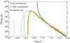Fig. 3 Distribution of the total GW abundance in the seventh NG15 frequency bin for the best-fit eccentricity model found in Sect. 7. The green (orange) curve shows the distribution obtained using the no-correlation (with correlations) method with 105 (104) realisations. The thick black dashed curve shows the analytical estimate of the long tail of the distribution of individual binaries. The dashed and dot-dashed curves show the contributions from strong and weak sources respectively.

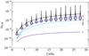Fig. 4 Best-fit eccentricity spectrum found in Sect. 7 (violins) and the means of the first 5 harmonics (solid curves) contributing towards the mean of the spectrum (solid black curve).

5.2 Correlations between frequencies

Since eccentric binaries emit GWs at several frequencies, they can contribute to more than one frequency bin and consequently make them correlated. To study these correlations, we needed to sample both Ω_c and e from (23). We, again, computed the total GW abundance in frequency bins, P(Ω|f_j), by dividing the sources into strong and weak sources. Here the threshold was on Ω_c instead of Ω and, since we needed to fix f₂ instead of the frequencies of the data bins, we binned f₂ so that each output (NG15) frequency bin was divided into 10 smaller frequency bins and both higher and lower frequencies were added to account for signal “leaking” into the PTA sensitivity range. We chose f₂ from each of the small input bins and sampled simultaneously Ω_c and e from (23). The expected number of binaries in a frequency interval (f_2,j, f_{2,j +1)} is $$N_j={\displaystyle {\int }_{f_j}^{f_{j+1}}\hspace{0.17em}\text{d}}\ln f_2\frac{\hspace{0.17em}\text{d}N}{\hspace{0.17em}\text{d\hspace{0.17em}}\ln f_2},$$(32)

and the number of strong sources is N_S,j = p_S,jN_j ≪ N_j, where $$p_{\text{S},j}={\displaystyle {\int }_{{\mathrm{\Omega }}_c^{(1)}>{\mathrm{\Omega }}_{\text{thr}}}\hspace{0.17em}\text{d}}e\hspace{0.17em}\text{d}{\mathrm{\Omega }}_c{P}^{(1)}\left({\mathrm{\Omega }}_c,e\mid f_j\right).$$(33)

The emission by each strong binary was binned into the data bins to get the total contribution from the strong sources: $${\mathrm{\Omega }}_{\text{S}}\left(f_j\right)=\frac{1}{\ln \left(f_{j+1}/f_j\right)}{\displaystyle \sum _{k=1}^{N_{\text{S}}}{\displaystyle \sum _{n\in N_j}\frac{{\mathrm{\Omega }}_{c,k}{g}_n\left(e_k\right)}{ℱ\left(e_k\right)}}},$$(34)

where k labels the strong binaries and n ∈ N_j = {2 f_j / f_{2, k},…, 2f_j+1/f_2,k} are the harmonics of each strong binary that contribute to the frequency bin f_j .

The correlation between the frequency bins i and j is given by $${\rho }_{ij}=\frac{\langle \mathrm{\Omega }\left(f_i\right)\mathrm{\Omega }\left(f_j\right)\rangle -\langle \mathrm{\Omega }\left(f_i\right)\rangle \langle \mathrm{\Omega }\left(f_j\right)\rangle }{{\sigma }_i{\sigma }_j},$$(35)

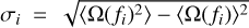where ${\sigma }_i=\sqrt{\langle \mathrm{\Omega }{\left(f_i\right)}^2\rangle -{\langle \mathrm{\Omega }\left(f_i\right)\rangle }^2}$. As shown in Fig. 3, the contribution from weak sources (dash-dotted yellow curve) is negligible in this approach. This is because for the computation of the correlations we considered 10 times more bins of the second harmonic frequency f₂ than in the computation based on the observed frequency, f, but we kept the number of strong sources in each bin the same. Consequently, the strong sources almost fully dominate the background and we can neglect the weak sources⁴.

Fig. 5 shows correlations between Ω(ƒ_i) in different frequency bins for various initial eccentricities in a SMBH model with p_BH = 1. The correlations depend on the amount of eccentricity present in the binary population, with the strongest correlations following a line of frequency ratio 2/3. This ratio dominates because the spectrum of moderately eccentric binaries tends to be dominated by the 2nd and the 3rd harmonics. When the 4th harmonic is included, then most of the correlations are expected to be found in the region between frequency ratios 3/4 and 1/2, highlighted by the turquoise band in Fig. 5. We found that the correlations can be negligible already for relatively large initial eccentricities 〈e〉_2nHz ≲ 0.5, while notable correlations required very high initial eccentricities 〈e〉_2nHz = 0.9. In such cases, the strongly correlated bins seen can appear away from the 1/2–3/4 ratio band due to the non-vanishing contribution from higher harmonics.

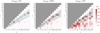Fig. 5 Correlations between frequency bins for spectra generated with 104 realisations, pBH = 1 and differing initial mean eccentricities at orbital frequency ƒb = 2 nHz. The correlations get stronger as eccentricity increases, with the strongest correlations found for frequency ratios 2/3 (along the blue dashed line) and most of the correlated bins are expected to lie between the ratios 3/4 and 1/2 (shaded blue area).

6 Environmental effects

In addition to GW emission, SMBH binaries may lose energy through dissipative environmental effects. The change in the binaries binding energy E is then $$\dot{E}=-{\dot{E}}_{\text{GW}}-{\dot{E}}_{\text{env}}.$$(37)

The impact of environmental effects is not fully known. Though it is generally expected that encounters with stars and drag due to circumbinary gas disks shorten binary inspiral times (Tang et al. 2017; Armitage & Natarajan 2002; Merritt 2013), some also argue that environmental effects can expand binary orbits (Muñoz et al. 2019). Following Ellis et al. (2024b), we introduced environmental effects via a phenomenological power-law ansatz.

The characteristic timescales for GW emission and environmental effect energy loss are t_GW = |E|/Ė_GW = 4τ and t_env = |E|/Ė_env, where τ is the coalescence time of the binary assuming only GW emission. Following Eq. (4), we see that $$t_{\text{GW}}=\frac{\left|E\right|}{{\dot{E}}_{\text{GW}}}=\frac{\left|E\right|}{{\dot{E}}_{\text{GW}}^cℱ(e)}=\frac{4{\tau }_c}{ℱ(e)},$$(38)

where τ_c = (5/256)(1 + z)(πƒ_r )^−8/3ℳ^−5/3 is the observed coalescence time of a circular binary, τ_c = lim_e→0 τ. By computing the time derivative of the binding energy E = − (π ƒ_r)^2/3 ℳ^5/3/2, the impact of environmental effects to the residence time of binaries at each logarithmic frequency can then be found to be $$\begin{array}{l}\frac{\text{d}t}{\text{d\hspace{0.17em}}\ln f_r}=\frac{2}{3}{\left(t_{\text{GW}}^{-1}+t_{\text{env}}^{-1}\right)}^{-1}\hfill \\ =\frac{2}{3}\frac{t_{\text{GW}}^c}{ℱ(e)}{\left[1+\frac{t_{\text{GW}}^c}{t_{\text{env}}}\frac{1}{ℱ(e)}\right]}^{-1},\hfill \end{array}$$(39)

giving $$\frac{\text{d}{E}_n}{\text{d\hspace{0.17em}}\ln f_r}={\frac{\text{d}{E}_n}{\text{d\hspace{0.17em}}\ln f_r}|}_{t_{\text{env\hspace{0.17em}}\to \infty }}{\left[1+\frac{t_{\text{GW}}^c}{t_{\text{env}}}\frac{1}{ℱ(e)}\right]}^{-1}.$$(40)

To leading order, the timescale of the environmental effects can be approximated with a power-law treatment $$\frac{t_{\text{env}}}{t_{\text{GW}}^c}={\left(\frac{f_r}{f_{\text{GW}}}\right)}^{\alpha },$$(41)

where ƒ_GW is the reference frequency above which GW emission becomes the dominant form of energy loss. We parametrize ƒ_GW as $$f_{\text{GW}}(ℳ,\eta ,z)=f_{\text{ref}}{\left(\frac{ℳ}{{10}^9{M}_{\odot }}\right)}^{-\beta }.$$(42)

The modified orbital evolution due to the introduction of environmental effects also has an effect on the evolution of eccentricity distributions as a function of orbital frequency, with Eq. (9) now becoming $$\frac{\text{d}e}{\text{d\hspace{0.17em}}\ln f_{\text{b}}}=-\frac{1}{288}\frac{\mathcal{G}(e)}{ℱ(e)}{\left[1+\frac{t_{\text{GW}}^c}{t_{\text{env}}}\frac{1}{ℱ(e)}\right]}^{-1}.$$(43)

Here we implicitly assumed that the environmental effects do not change the evolution of binary eccentricity, i.e., de/dt_r is still given by Eq. (6)⁵.

The evolution of the eccentricity distribution now depends on the masses of the binary components. Our numerical estimates suggested that environmental effects affected the eccentricity evolution of light-to-moderate binaries. As an explicit example, we considered a scenario with the environmental parameters fixed to the best-fit values obtained in Ellis et al. (2024c) and an initial eccentricity of 〈e〉_2nHz = 0.80. Independently of the binary mass, the mean eccentricity in the last bin was 〈e〉_{28 nHz} = 0.40 when no environmental effects were present. When environmental effects were included 〈e〉_28nHz = 0.41 for binaries with ℳ = 10¹⁰M_⊙, 〈e〉_{28 nHz} = 0.67 for binaries with ℳ = 10⁸M_⊙ and the mean eccentricity of light binaries, ℳ ≲ 10⁶M_⊙, remained practically constant at all bins indicating that orbital evolution is almost entirely dominated by environmental effects. It follows that, since light binaries exhibit no evolution of mean eccentricity as a function of orbital frequency, their contribution to the final spectrum is uniformly suppressed and becomes even less significant.

In both Eqs. (40) and (43), the environmental effect terms are scaled by a ℱ⁻¹(e) factor. Since ℱ(e) ≥ 1, environmental effects are suppressed for highly-eccentric binaries and, for most of the parameter space, the evolution of binaries is either eccentricity or environment-dominated.

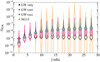Fig. 6 Best fits assuming energy loss by only GWs (black), energy loss by GWs and environmental effects (Ellis et al. 2024b) (pink) and energy loss by GWs from eccentric binaries (green) compared to the NG15 data (yellow).

7 Fit to the PTA data

We analysed the model against the NG15 data using the likelihood $$l\left({\mathit{\theta }}_f\right)\propto {\displaystyle \underset{i}{\prod \text{}}}{{\displaystyle \int }}^{\text{}}\text{dΩ}{P}_{\text{data}}\left(\text{Ω}\mid f_i\right)P\left(\text{Ω}\mid f_i,{\mathit{\theta }}_f\right),$$(44)

where the product is over the NG15 frequency bins, P_data(Ω|ƒ_i) are the probability distribution functions of the Hellings-Down- correlated free spectrum fit (Agazie et al. 2023a) (i.e., the NG15 violins shown in Fig. 6) and θ_ƒ denotes the model parameters. The full model presented in this paper, including both environmental effects and eccentricity, contains 5 free parameters: θ_ƒ = {p_BH, 〈e〉_2nHz,α, β, ƒ_ref}. Because of the large parameter space and increasingly complex integral for P⁽¹⁾(Ω| ƒ), a full fit of the model to the NG15 data was computationally unfeasible. In the following, we performed fits without environmental effects and with fixed values of α, β and ƒ_ref. To compare models we introduced the likelihood ratio $${\ell }_{\max }=\frac{{\max }_{{\mathit{\theta }}_f}l\left({\mathit{\theta }}_f\mid H_1\right)}{{\max }_{{\mathit{\theta }}_f}l\left({\mathit{\theta }}_f\mid H_2\right)}.$$(45)

where H₁ and H₂ label the models.

We performed a scan of the parameter space for the model containing only eccentricity effects, t_env ≫ t_Gw, with θ_ƒ = {p_BH, 〈e〉_{2 nHz}}. The maximal likelihood analysis yielded best- fit values of p_BH = 0.60 and 〈e〉_{2 nHz} = 0.83 (corresponding to the power-law index γ_2nHz = 3.9). The 1σ, 2σ and 3σ confidence levels of the two-dimensional likelihood are shown in Fig. 7 by the coloured regions. The fit prefers values of the SMBH merger efficiency, p_BH > 0.17 and the likelihood peaks sharply around an initial eccentricity of ≈0.83 due to fitting the low-frequency dip of the NG15 data. At low eccentricities, the contours bend towards the black square, indicating the best fit for circular GW driven binaries. This point is disfavoured by more than 3σ compared to the fit with eccentric binaries.

For the second scan, we fixed α = 8/3, β = 5/8 and ƒ_ref = 30 nHz. This choice of α and β corresponds to gas infall driven binary evolution (Begelman et al. 1980) and the choice of ƒ_ref gives a good fit to the NG15 data assuming circular binaries (Ellis et al. 2024c). Performing the likelihood analysis in θ_ƒ = {p_BH, 〈e〉_{2 nHz}} yielded the dashed contours seen in Fig. 7. The 1σ region now extends from highly eccentric binaries down to circular binaries. The highest likelihoods are still found at very high eccentricities and near-maximal values of p_BH. At high eccentricities, the environmental effects are rendered insignificant due to the suppression factor in Eq. (40) and confidence regions become increasingly similar to the scenario without environmental effects.

In Fig. 6, we show the best-fit spectra of the models with GW-driven circular binaries, circular binaries with environmental effects and GW-driven eccentric binaries. The parameter values are collected in Table 1. The resulting spectrum in the eccentricity model is similar to the spectrum generated by the environmental effects, but the violins are much narrower due to the higher p_BH needed. The likelihood ratios reported in Table 1 imply that the eccentricity model provides a slightly better fit than the circular binary model with environmental effects.

Fig. 7 Fit of the eccentric SMBH binary model (solid) and a model with fixed environmental parameters (ƒref = 30nHz, α = 8/3,β = 5/8) with added eccentricity (dashed). Note that the confidence levels are shown for each fit separately, with the ratio between the 1σ contours of the purely eccentric and environmental+eccentricity model being ≈5. The black circle denotes the best-fit point in the model including eccentricities, while the black square/star indicate the best-fit points for circular binaries with environmental effects omitted/included.

8 Conclusions

We presented a semi-analytic method for computing the stochastic gravitational wave background spectrum generated by a population of inspiraling eccentric supermassive black hole binaries expanding upon the work done in Ellis et al. (2024b, 2023, 2024c). Since eccentric binaries spend less time emitting GWs at each frequency, the resulting gravitational wave spectrum of SMBH binaries is generally suppressed depending on the amount of eccentricity present in the SMBH binary population. However, as GW emission tends to circularize orbits, binaries with smaller separations tend to be less eccentric, leading to stronger suppression in the low-frequency tail of the spectrum. We find that this suppression is near-degenerate with the effects of environmental interactions.

We found that the NANOGrav 15-year observations prefer very high initial eccentricities of around 〈e〉_{2 nHz} = 0.83 if the evolution of SMBH binaries in the PTA frequency range is driven purely by gravitational wave emission. When environmental effects are present, the mean eccentricity preferred by data is greatly reduced although non-vanishing eccentricities are still mildly preferred. Our main results are summarized in Fig. 7.

Although eccentricity and environmental effects tend to produce very similar spectral modulations, we found they can differ in a few key aspects: (i) The fit of the eccentricity model without environmental effects prefers smaller spectral fluctuations compared to the fit of circular binaries with environmental effects. (ii) As eccentric binaries do not emit monochromatically, they will generate correlations between different frequency bins that can be sizeable for relatively large (〈e〉_{2 nHz} ≳ 0.5) initial eccentricity and they cannot be mimicked by environmental effects. These effects provide a potential way to distinguish whether eccentricities or environmental interactions have the dominant effect on the spectral shape of the PTA GW signal.

Acknowledgments

This work was supported by the Estonian Research Council grants PRG803, PSG869, RVTT3 and RVTT7 and the Center of Excellence program TK202. The work of V.V. was partially supported by the European Union’s Horizon Europe research and innovation program under the Marie Skłodowska-Curie grant agreement No. 101065736.

References

All Tables

All Figures

	Fig. 1 Evolution of an eccentricity distribution set to be uniform at f = f0. The inset shows the evolution of the expectation value of e.
In the text

	Fig. 2 Function E defined in (21) that describes the modification of the mean GW spectrum caused by the binary eccentricities shown for power-law (solid) and delta function (dashed) initial eccentricity distributions and different values of mean eccentricity of the initial distribution fixed at f = f0.
In the text

Fig. 3 Distribution of the total GW abundance in the seventh NG15 frequency bin for the best-fit eccentricity model found in Sect. 7. The green (orange) curve shows the distribution obtained using the no-correlation (with correlations) method with 105 (104) realisations. The thick black dashed curve shows the analytical estimate of the long tail of the distribution of individual binaries. The dashed and dot-dashed curves show the contributions from strong and weak sources respectively.

In the text

	Fig. 4 Best-fit eccentricity spectrum found in Sect. 7 (violins) and the means of the first 5 harmonics (solid curves) contributing towards the mean of the spectrum (solid black curve).
In the text

Fig. 5 Correlations between frequency bins for spectra generated with 104 realisations, pBH = 1 and differing initial mean eccentricities at orbital frequency ƒb = 2 nHz. The correlations get stronger as eccentricity increases, with the strongest correlations found for frequency ratios 2/3 (along the blue dashed line) and most of the correlated bins are expected to lie between the ratios 3/4 and 1/2 (shaded blue area).

In the text

	Fig. 6 Best fits assuming energy loss by only GWs (black), energy loss by GWs and environmental effects (Ellis et al. 2024b) (pink) and energy loss by GWs from eccentric binaries (green) compared to the NG15 data (yellow).
In the text

Fig. 7 Fit of the eccentric SMBH binary model (solid) and a model with fixed environmental parameters (ƒref = 30nHz, α = 8/3,β = 5/8) with added eccentricity (dashed). Note that the confidence levels are shown for each fit separately, with the ratio between the 1σ contours of the purely eccentric and environmental+eccentricity model being ≈5. The black circle denotes the best-fit point in the model including eccentricities, while the black square/star indicate the best-fit points for circular binaries with environmental effects omitted/included.

In the text

References

- Agazie, G., Anumarlapudi, A., Archibald, A., et al. 2023a, ApJ, 951, L8 [NASA ADS] [CrossRef] [Google Scholar]
- Agazie, G., Anumarlapudi, A., Archibald, A., et al. 2023b, ApJ, 951, L9 [CrossRef] [Google Scholar]
- Antoniadis, J., Babak, S., Bak Nielsen, A.-S., et al. 2023a, A&A, 678, A48 [Google Scholar]
- Antoniadis, J., Babak, S., Bak Nielsen, A.-S., et al. 2023b, A&A, 678, A50 [CrossRef] [EDP Sciences] [Google Scholar]
- Antoniadis, J., Babak, S., Bak Nielsen, A.-S., et al. 2024, A&A, 685, A94 [NASA ADS] [CrossRef] [EDP Sciences] [Google Scholar]
- Armitage, P. J., & Natarajan, P. 2002, ApJ, 567, L9 [NASA ADS] [CrossRef] [Google Scholar]
- Begelman, M. C., Blandford, R. D., & Rees, M. J. 1980, Nature, 287, 307 [Google Scholar]
- Berczik, P., Merritt, D., Spurzem, R., & Bischof, H.-P. 2006, ApJ, 642, L21 [Google Scholar]
- Bi, Y.-C., Wu, Y.-M., Chen, Z.-C., & Huang, Q.-G. 2023, Sci. China Phys. Mech. Astron., 66, 120402 [NASA ADS] [CrossRef] [Google Scholar]
- Bond, J. R., Cole, S., Efstathiou, G., & Kaiser, N. 1991, ApJ, 379, 440 [NASA ADS] [CrossRef] [Google Scholar]
- Chen, S., Sesana, A., & Del Pozzo, W. 2017, MNRAS, 470, 1738 [CrossRef] [Google Scholar]
- D’Orazio, D. J., & Duffell, P. C. 2021, ApJ, 914, L21 [CrossRef] [Google Scholar]
- Dotti, M., Colpi, M., Haardt, F., & Mayer, L. 2007, MNRAS, 379, 956 [NASA ADS] [CrossRef] [Google Scholar]
- Eisenstein, D. J., & Hu, W. 1998, ApJ, 496, 605 [Google Scholar]
- Ellis, J., Fairbairn, M., Hütsi, G., et al. 2023, A&A, 676, A38 [NASA ADS] [CrossRef] [EDP Sciences] [Google Scholar]
- Ellis, J., Fairbairn, M., Franciolini, G., et al. 2024a, Phys. Rev. D, 109, 023522 [NASA ADS] [CrossRef] [Google Scholar]
- Ellis, J., Fairbairn, M., Hütsi, G., et al. 2024b, Phys. Rev. D, 109, L021302 [NASA ADS] [CrossRef] [Google Scholar]
- Ellis, J., Fairbairn, M., Hütsi, G., et al. 2024c, arXiv e-prints [arXiv:2403.19650] [Google Scholar]
- Enoki, M. & Nagashima, M. 2007, Prog. Theor. Phys., 117, 241 [CrossRef] [Google Scholar]
- Fastidio, F., Gualandris, A., Sesana, A., Bortolas, E., & Dehnen, W. 2024, MNRAS, accepted [arXiv:2406.02710] [Google Scholar]
- Girelli, G., Pozzetti, L., Bolzonella, M., et al. 2020, A&A, 634, A135 [NASA ADS] [CrossRef] [EDP Sciences] [Google Scholar]
- Gualandris, A., Khan, F. M., Bortolas, E., et al. 2022, MNRAS, 511, 4753 [NASA ADS] [CrossRef] [Google Scholar]
- Hellings, R. w., & Downs, G. s. 1983, ApJ, 265, L39 [NASA ADS] [CrossRef] [Google Scholar]
- Huerta, E. A., McWilliams, S. T., Gair, J. R., & Taylor, S. R. 2015, Phys. Rev. D, 92, 063010 [NASA ADS] [CrossRef] [Google Scholar]
- Jeans, J. H. 1919, MNRAS, 79, 408 [NASA ADS] [CrossRef] [Google Scholar]
- Kelley, L. Z., Blecha, L., Hernquist, L., Sesana, A., & Taylor, S. R. 2017, MNRAS, 471, 4508 [NASA ADS] [CrossRef] [Google Scholar]
- Lacey, C., & Cole, S. 1993, MNRAS, 262, 627 [NASA ADS] [CrossRef] [Google Scholar]
- Merritt, D. 2013, Class. Quant. Grav., 30, 244005 [NASA ADS] [CrossRef] [Google Scholar]
- Miranda, R., Muñoz, D. J., & Lai, D. 2017, MNRAS, 466, 1170 [NASA ADS] [CrossRef] [Google Scholar]
- Muñoz, D. J., Miranda, R., & Lai, D. 2019, ApJ, 871, 84 [CrossRef] [Google Scholar]
- Nasim, I., Gualandris, A., Read, J., et al. 2020, MNRAS, 497, 739 [Google Scholar]
- Peters, P. C., & Mathews, J. 1963, Phys. Rev., 131, 435 [Google Scholar]
- Phinney, E. S. 2001, arXiv e-prints [arXiv:astro-ph/0108028] [Google Scholar]
- Planck Collaboration VI. 2020, A&A, 641, A6 [NASA ADS] [CrossRef] [EDP Sciences] [Google Scholar]
- Press, W. H., & Schechter, P. 1974, ApJ, 187, 425 [Google Scholar]
- Rawlings, A., Mannerkoski, M., Johansson, P. H., & Naab, T. 2023, MNRAS, 526, 2688 [NASA ADS] [CrossRef] [Google Scholar]
- Reardon, D. J., Zic, A., Shannon, R., et al. 2023a, ApJ, 951, L6 [NASA ADS] [CrossRef] [Google Scholar]
- Reardon, D. J., Zic, A., Shannon, R., et al. 2023b, ApJ, 951, L7 [NASA ADS] [CrossRef] [Google Scholar]
- Sesana, A. 2013, Class. Quant. Grav., 30, 224014 [NASA ADS] [CrossRef] [Google Scholar]
- Tang, Y., MacFadyen, A., & Haiman, Z. 2017, MNRAS, 469, 4258 [Google Scholar]
- Vasiliev, E., Antonini, F., & Merritt, D. 2015, ApJ, 810, 49 [Google Scholar]
- Xu, H., Chen, S., Guo, Y., et al. 2023, Res. Astron. Astrophys., 23, 075024 [CrossRef] [Google Scholar]
- Zic, A., Reardon, D. J., Kapur, A., et al. 2023, PASA, 40, e049 [NASA ADS] [CrossRef] [Google Scholar]
- Zrake, J., Tiede, C., MacFadyen, A., & Haiman, Z. 2021, ApJ, 909, L13 [NASA ADS] [CrossRef] [Google Scholar]
Geometric units c = G = 1 are used throughout the paper.
We computed the variance of smoothed mass fluctuations following Eisenstein & Hu (1998) and used the values of the cosmological parameters inferred from the CMB observations (Planck Collaboration VI 2020).
The factor of (2/n)2/3 arises from changing orbital frequencies from fb = fr/n to fb = fr/2 in Eq. (19).
Correlations between the frequency bins of the weak source background can be described by a multivariate Gaussian
![Mathematical equation: $\eqalign{ & P\left( {{\Omega _{\rm{W}}}\left( {{f_1}} \right),{\Omega _{\rm{W}}}\left( {{f_2}} \right), \ldots ,{\Omega _{\rm{W}}}\left( {{f_j}} \right)} \right) \cr & \,\,\,\,\,\,\,\,\,\,\, \approx {{\exp \left[ { - {{\left( {{{\bf{\Omega }}_{\rm{W}}} - \left\langle {{{\bf{\Omega }}_{\rm{W}}}} \right\rangle } \right)}^T}{{\bf{\Sigma }}^{ - 1}}({{\bf{\Omega }}_{\rm{W}}} - \langle {{\bf{\Omega }}_{\rm{W}}})\rangle } \right]} \over {\sqrt {{{(2\pi )}^j}|{\bf{\Sigma }}|} }}, \cr} $](/articles/aa/full_html/2024/11/aa51345-24/aa51345-24-eq56.png) (36)
(36)
where j is the number of bins, Σ is the covariance matrix and 〈ΩW〉 is the vector of mean ΩW in each bin. The covariance matrix of the multivariate normal distribution is then Σ¡j ∈ σiσjρ¡j where  .
.
A similar approach is adopted in Chen et al. (2017, Eq. (31)), where eccentricity evolution below a threshold frequency was turned off. Instead of a sharp cutoff, Eq. (43) adopts a more gradual suppression of the eccentricity evolution.
All Tables
Log-likelihood differences and the posterior means and standard deviations for the considered parametrizations.