| Issue |
A&A
Volume 676, August 2023
|
|
|---|---|---|
| Article Number | A115 | |
| Number of page(s) | 10 | |
| Section | Cosmology (including clusters of galaxies) | |
| DOI | https://doi.org/10.1051/0004-6361/202345911 | |
| Published online | 18 August 2023 | |
Unraveling the formation histories of the first supermassive black holes with the Square Kilometre Array’s pulsar timing array
1
Département de Physique Théorique, Université de Genève, 24 quai Ernest-Ansermet, 1211 Genève 4, Switzerland
e-mail: This email address is being protected from spambots. You need JavaScript enabled to view it.
2
Astronomy department, Harvard University, 60 Garden Street, Cambridge, MA 02138, USA
e-mail: This email address is being protected from spambots. You need JavaScript enabled to view it.
Received:
13
January
2023
Accepted:
28
May
2023
Abstract
Galaxy mergers at high redshifts trigger activity of their central supermassive black holes, eventually also leading to their coalescence as well as a potential source of low-frequency gravitational waves detectable by the Square Kilometre Array’s pulsar timing array (SKA PTA). Two key parameters related to the fueling of black holes are the Eddington ratio of quasar accretion, ηEdd, and the radiative efficiency of the accretion process, ϵ (which affects the so-called active lifetime of the quasar, tQSO). Here, we forecast the regime of detectability of gravitational wave events with SKA PTA. We find the associated binaries to have orbital periods of the order of weeks to years, observable via relativistic Doppler velocity boosting and/or optical variability of their light curves. Combining the SKA regime of detectability with the latest observational constraints on high-redshift black hole mass and luminosity functions, as well as theoretically motivated prescriptions for the merger rates of dark matter halos, we forecast the number of active counterparts of SKA PTA events expected as a function of primary black hole mass at z ≳ 6. We find that the quasar counterpart of the most massive black holes will be uniquely localizable within the SKA PTA error ellipse at z ≳ 6. We also forecast the number of expected counterparts as a function of the quasars’ Eddington ratios and active lifetimes. Our results show that SKA PTA detections can place robust constraints on the seeding and growth mechanisms of the first supermassive black holes.
Key words: galaxies: high-redshift / quasars: supermassive black holes / gravitational waves
© The Authors 2023
 Open Access article, published by EDP Sciences, under the terms of the Creative Commons Attribution License (https://creativecommons.org/licenses/by/4.0), which permits unrestricted use, distribution, and reproduction in any medium, provided the original work is properly cited.
This article is published in open access under the Subscribe to Open model. This email address is being protected from spambots. You need JavaScript enabled to view it. to support open access publication.
1. Introduction
The seeding and growth of the first supermassive black holes in the Universe represent an outstanding question in contemporary astrophysics (Rees 1984; Turner 1991; Barkana & Loeb 2001). There currently exists an observational sample of 213 quasars1 at z > 6 from current surveys (for the latest collection and a “live” catalog, see, e.g., Flesch 2021). The masses of the supermassive black holes associated with the observed quasars follow a broad distribution (Fig. 1) between 108 M⊙ < MBH < 1010 M⊙, with most observed to be in a rapidly accreting phase having Eddington ratios close to unity (Fan et al. 2006; Wu et al. 2015; Kim & Im 2019; Millon et al. 2022; Venemans et al. 2016, 2017; Willott et al. 2015; Trakhtenbrot et al. 2017; Bañados et al. 2018; Feruglio et al. 2018; Mortlock et al. 2011; De Rosa et al. 2014). For a reasonable range of seed values, the maximum mass of a black hole at any redshift is predicted to be 1010 M⊙ (Haiman & Loeb 2001; Natarajan & Treister 2009; Inayoshi & Haiman 2016; King 2016), which is consistent with the value established for the most massive black hole at z > 6 discovered so far (∼1.2 × 10¹⁰ M⊙; Wu et al. 2015). When combined with the inferred lifetimes of quasars (Eilers et al. 2020, 2021; Khrykin et al. 2021; Volonteri 2010, 2012), this leads to the question of how such massive systems grew over a relatively short period in the history of the Universe (for a review, see Inayoshi et al. 2020).
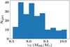 |
Fig. 1. Distribution of estimated black hole masses in observed z > 6 quasars. Masses are derived from bolometric luminosities (when available), assuming Eddington ratios from Nobuta et al. (2012). These are also consistent with mass estimates derived independently in the literature. |
In addition to the black hole mass, two key physical parameters that determine the black hole seeding and growth mechanisms are the bolometric luminosity, Lbol, of the associated quasar (usually expressed in units of the Eddington luminosity, LEdd = 1.3 × 1038(MBH/M⊙)L⊙, as ηEdd = Lbol/LEdd) and the radiative efficiency of accretion of material on to the black hole, ϵ, which is believed to power nuclear activity and is related (Pacucci & Loeb 2022) to the active lifetime of the quasar, tQSO. The combination of ηEdd and ϵ is constrained by the Salpeter time-scale (tS; Salpeter 1964) for black hole growth, which can be expressed as tS = 0.45(ϵ/1 − ϵ)(Lbol/LEdd)−1 Gyr. The mass of the black hole grows exponentially according to MBH = Mseedexp(tQSO/tS) – starting from a seed mass, Mseed, which could have different possible origins that range from remnants of Pop III stars (Madau & Rees 2001), primordial black holes from the early Universe (Carr & Hawking 1974), or “heavy” seeds formed from direct collapse of gas clouds (Haehnelt & Rees 1993; Bromm & Loeb 2003; Lodato & Natarajan 2006, 2007; Agarwal et al. 2016; Pacucci et al. 2017; Natarajan et al. 2017; Bonoli et al. 2014).
In the hierarchical structure formation scenario, galaxy mergers are expected to be frequent at z ≳ 6, leading to the inevitable formation of binary supermassive black holes (SMBHs). There is, however, a considerable level of uncertainty with respect to our understanding of the evolution of such systems (e.g., Begelman et al. 1980; Armitage & Natarajan 2002; Milosavljević & Merritt 2003; Kulkarni & Loeb 2012), especially in terms of their lifetimes and coalescence timescales. The latter is especially important in view of observational signatures, such as the gravitational wave emission that is expected to accompany the final stages of coalescence (Peters 1964; Loeb 2010).
Pulsar timing arrays are aimed at detecting a gravitational wave background at low frequencies by monitoring the spatially correlated fluctuations induced by the waves on the times of arrival (ToA) of radio pulses from millisecond pulsars. A key astrophysical source of such a stochastic background is that generated by a cosmic population of SMBH binaries (e.g., Sesana et al. 2004; Burke-Spolaor et al. 2019; Maiorano et al. 2021; Rajagopal & Romani 1995; Rosado et al. 2016; Wen et al. 2011; Bonetti et al. 2018; Feng et al. 2020), which emit gravitational waves with frequencies of the order of a few nHz, once the separation reaches sub-pc scales2.
The Square Kilometre Array (SKA) will revolutionize gravitational wave astronomy with pulsar timing (Stappers et al. 2018; Kramer 2004; Janssen et al. 2015), thanks to its much larger collecting area and improved sensitivity to frequencies of the order of the reciprocal of the observing time, namely, nHz for observing timescales of a few years. A pulsar timing array (PTA) with the SKA has been predicted to have the capacity to discover more than 14 000 canonical and 6000 millisecond pulsars within the first five to eight years of operation (Smits et al. 2009; Taylor et al. 2016; Cordes et al. 2004; Rosado et al. 2015). It also has the potential to bring down the precision on timing the residuals (computed from the phase difference between the observed ToA and the predicted ToA based on model parameters) to 1–10 ns (Liu et al. 2011; Spallicci 2013). Sensitive to frequencies between 1 nHz and 100 nHz, the SKA PTA will significantly boost (Kramer 2004; Janssen et al. 2015) the existing efforts from the International PTA collaboration (IPTA; Verbiest et al. 2016) to detect low-frequency gravitational waves, complementing the regime probed by the LIGO, Advanced Virgo and KAGRA (Hz), and LISA (mHz) facilities.
In this paper, we outline the prospects for detecting SMBH mergers at redshifts z ≳ 6 from their gravitational wave signal measured by the SKA PTA. In so doing, we provide fully data-driven expressions for the proportion of active quasars among black holes at high redshifts, as well as the fraction of binary SMBHs. The SMBH binaries’ contribution to the background, expected to be the brightest in the PTA band, can be robustly isolated within a few years of integration (Pol et al. 2021; Kaiser et al. 2022). We find that SKA PTA should be sensitive to SMBHs with primary black hole masses of MBH ≳ 109 M⊙, mass ratios greater than qmin = 0.25 (for MBH ∼ 109 M⊙) and qmin = 0.005 (for MBH ∼ 1010 M⊙) and separations of a = 0.5 − 50 mpc, fairly independently of redshift. Assuming that the black hole mergers proceed rapidly to coalescence, we forecast the expected number of detections and their electromagnetic counterparts – both quasars (Kocsis et al. 2006; Casey-Clyde et al. 2022) and galaxies (Haiman et al. 2009) detectable by current and future facilities. We explore the implications of our findings for placing constraints on the parameters ηEdd and tQSO that are related to the growth mechanisms of black holes. In so doing, we provide fully data-driven expressions for the proportion of active quasars among black holes at high redshifts, as well as the fraction of binary SMBHs as a function of observationally determined parameters.
The paper is organized as follows. In Sect. 2, we develop the formalism connecting the observed strain and frequency of SKA PTA measurements to the properties of high redshift SMBHs. Using theoretically motivated prescriptions for the merger rates of dark matter haloes with empirically derived constraints on their black hole masses, we forecast the number of binary SMBHs detectable by SKA PTA via their gravitational wave emission. In Sect. 3, we outline prospects for detecting the electromagnetic counterparts of these sources, including both galaxies (Sect. 3.1) and QSOs (Sect. 3.2), including predictions for the number of active QSO counterparts expected as a function of black hole properties at z > 6. We summarize our findings in Sect. 4.
2. Gravitational wave constraints on supermassive black holes
The expected sensitivity of SKA PTA as a function of the observed frequency is shown by the blue curve in Fig. 2, derived from the estimates of Garcia-Bellido et al. (2021). The cited estimates are based upon a nominal sensitivity level of 10−16 − 10−17 at the reference frequency of 1 yr−1. This curve assumes 50 pulsars timed every two weeks for 20 years with a root-mean-square error in each timing residual of 30 ns from Moore et al. (2015). Typically, the three observables: strain, h, frequency, fobs, and the gravitational wave decay timescale, tgw, obs, may be measurable in the PTA survey. For an SMBH binary of masses, M1 and M2 (assumed to be less than or equal to M1), with a separation of a, and located at redshift, z, the strain and observed frequency can be expressed as:
 (1)
(1)
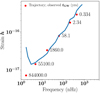 |
Fig. 2. Strain vs. observed frequency of SKA PTA (blue curve, from Garcia-Bellido et al. 2021). The red dots mark example points on the trajectory of a binary system at z ∼ 6.8 with masses of M1 = 1010 M⊙ and M2 ≈ 3 × 10⁷ M⊙ as a function of the gravitational wave decay timescale, tGW, measured in units of years in the observer’s frame of reference. |
In the above equations, ℳobs denotes the observed chirp mass, defined by ℳobs = (M1M2)3/5(1 + z)/(M1 + M2)1/5, and dL is the luminosity distance to redshift, z.
The above equations can be used along with the SKA sensitivity curve to forecast constraints on the separation and minimum mass ratio of the black holes. This is done by considering two fiducial primary BH masses, M1 = 109 and 1010 M⊙, assumed to be located at a range of redshifts between z ∼ 1 and z ∼ 10. We solved Eq. (1) to derive the lower limits on the mass ratio (q = M2/M1) for both cases, as a function of the separation, a, allowing the strain versus frequency curve to be translated into the q − a plane (as shown in Figs. 3 and 4).
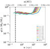 |
Fig. 3. Constraints on the q − a plane from the SKA sensitivity curve and assuming a primary black hole mass M1 = 109 M⊙ at various redshifts. The dashed line shows the innermost stable circular orbit (ISCO). |
A few comments on the qualitative behaviour of the curves in the q − a plane are in order. In Eq. (1) the relation  is implied, which can be approximated in the regime of M2 ≪ M1) as
  . Hence, for a given strain, h, and separation, a, we obtain M2 ∝ dL/(1 + z). For a fixed fobs, a is fixed up to a (1 + z) factor in the M2 ≪ M1 regime. The (1 + z) effect shows up as the linear shift in curves (at fixed q) as z is varied (the shift is by a factor of ∼5 from the highest to the lowest redshift). This leads to a very modest change (by a factor of order ∼3) in q as z varies from 1 to 10, as can be seen from Figs. 3 and 4. Thus, the range of secondary black hole masses constrainable by the SKA varies only mildly with a at all redshifts, with the minimum mass ratio qmin ∼ {0.25, 0.005} for M1 = {109, 1010} M⊙, respectively. The other important finding is that primary black hole masses lower than M1 ∼ 109 M⊙ are undetectable by the SKA at all redshifts of z ≳ 1. Across the range of redshifts, the most relevant for unravelling the growth history of black holes is the one closest to the highest redshift quasars, whose electromagnetic counterparts may allow for robust determinations of the source properties.
We now replot the constraints on the q − a plane obtained from the primary black hole assumed to be located at z ∼ 6.8, which is the redshift of the most luminous quasar detected so far. This is shown in Figs. 5 and 6. In each case, the observed orbital time period of the binary for the preferred mass ratio (q = 0.25 and q = 0.005, respectively) is indicated as a function of separation:
 (2)
(2)
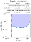 |
Fig. 5. Constraints on the q − a plane from the SKA sensitivity curve and assuming a primary black hole mass M1 = 109 M⊙ at z ∼ 6.8. The dashed line shows the innermost stable circular orbit (ISCO), while the shaded region indicates the regime of detectability of the binary SMBH with SKA PTA The top axes show the observed gravitational wave decay time and the orbital period of the binary and the velocity of the lower-mass black hole. The range of velocities in the regime of detectability is of the order of 0.06c − 0.2c, ensuring good prospects for prompt electromagnetic follow-ups via Doppler boosting of the light curves. |
Also shown is the observed gravitational wave emission (or binary decay) time:
 (3)
(3)
and the velocity of the lower-mass black hole (in units of c, assuming a circular orbit, e.g., D’Orazio et al. 2015b):
 (4)
(4)
and torbit, rest is derived from Eq. (2) by dividing by (1 + z).
We can calculate the number of binary black holes expected at z ∼ 6 as a function of mass ratio by using the formalism for the merger rate of dark matter halos per unit redshift (z) and halo mass fraction (ξ), as formulated by Fakhouri et al. (2010):
![Mathematical equation: $$ \begin{aligned} \frac{\mathrm{d} n_{\rm halo}}{\mathrm{d}z \mathrm{d}\xi }&= A \left(\frac{M_{\rm h}}{10^{12}\,M_{\odot }}\right)^{\alpha } \xi ^{\beta } \exp \left[\left(\frac{\xi }{\bar{\xi }}\right)^{\gamma _1}\right] (1+ z)^{\eta } ,\end{aligned} $$](/articles/aa/full_html/2023/08/aa45911-23/aa45911-23-eq7.gif) (5)
(5)
where Mh is the halo mass. In the above equation, the best-fitting parameters constructed from the halo merger trees have the values α = 0.133, β = −1.995, γ1 = 0.263, η = 0.0993, A = 0.0104, and  . Substituting the empirically constrained black hole-halo mass relation (e.g., Wyithe & Loeb 2002):
 (6)
(6)
in which log10ϵ0 = −5.02, γ = 4.53 (e.g., Padmanabhan & Loeb 2020), we derive:
![Mathematical equation: $$ \begin{aligned} \frac{\mathrm{d} N_{\rm BH,mrg}}{\mathrm{d}z \mathrm{d}q}&= A_1 f_{\rm bh} \left(\frac{M_{\rm h}}{10^{12}\,M_{\odot }} \right)^{\alpha } \nonumber \\&\quad \times q^{3/\gamma - 1 +3\beta /\gamma } (1+z)^{\eta } \exp \left[\left(\frac{q}{\bar{q}}\right)^{3\gamma _1/\gamma }\right] .\end{aligned} $$](/articles/aa/full_html/2023/08/aa45911-23/aa45911-23-eq10.gif) (7)
(7)
In the above expression, fbh denotes the fraction of dark matter haloes occupied by black holes, and q is the black hole mass ratio, related to ξ as q = ξγ/3,  and A1 = (3/γ)A. From this, we can define the number of binary black hole mergers expected per unit comoving volume as:
![Mathematical equation: $$ \begin{aligned} \frac{\mathrm{d} n_{\rm BHB}}{\mathrm{d}z \mathrm{d}q \mathrm{d} \log _{10} M_{\rm BH}}&= A_1 f_{\rm bh} \frac{3}{\gamma } \left(\frac{M_{\rm h}(M_{\rm BH})}{10^{12}\,M_{\odot }} \right)^{\alpha } \nonumber \\&\quad \times q^{3/\gamma - 1 +3\beta /\gamma } (1+z)^{\eta } \exp \left[\left(\frac{q}{\bar{q}}\right)^{3\gamma _1/\gamma }\right] \frac{\mathrm{d}n_{\rm h}}{\mathrm{d} \log _{10} M_{\rm h}} ,\end{aligned} $$](/articles/aa/full_html/2023/08/aa45911-23/aa45911-23-eq12.gif) (8)
(8)
in which the dnh/dlog10Mh term represents the dark matter halo mass function (taken to follow Sheth & Tormen 2002) and Mh(MBH) denotes the dark matter halo mass expressed as a function of black hole mass, obtained by inverting Eq. (6). The number density of gravitational wave events can now be found by multiplying the above expression by tgw(agr)(dz/dt), where tgw(agr) is the gravitational wave decay timescale in the rest frame of the binary; which, for the masses, M1 and M2 is given by Eq. (3) divided by (1 + z). It is evaluated at the scale agr – the radius at which emission of gravitational waves takes over as the dominant channel of coalescence – which is defined by:
 (9)
(9)
with
 (10)
(10)
and where we have:
 (11)
(11)
as the hardening scale of the binary (e.g., Merritt 2000; Kulkarni & Loeb 2012). In both of the above expressions, σ represents the one-dimensional velocity dispersion of the primary host galaxy, which is related to its black hole mass by (Tremaine et al. 2002):
 (12)
(12)
with γ as defined in Eq. (6). For each of the candidate primary black hole masses above, we can integrate the expression over the requisite q-range to find the total number of binary SMBHs, ϕBHB, gw(MBH, qmin), expected per unit of comoving volume. Assuming the binary merger proceeds to coalescence without delay (Fang & Yang 2023), we find:
 (13)
(13)
over the q-range, starting from the minimum value of q under consideration. In the case of the SKA, for example, qmin ∼ 0.25 when MBH = 109 M⊙ and qmin ∼ 0.005 when MBH = 1010 M⊙, fairly independently of the separation (as shown in Fig. 3).
From Eq. (13), we can obtain the total number of black hole binaries in a given redshift interval:
 (14)
(14)
where dV represents the comoving volume under consideration. All the above expressions are generic and valid for the whole range of redshift and primary black hole mass values. In particular, they can be used to compute the number of the number of binaries detectable by the SKA PTA around z ∼ 6.8 and over the interval 6 < z < 7.1, for both the primary black hole masses considered earlier along with their corresponding qmin values. This is indicated on the third column of Table 1. The quantities are also a function of the solid angle on the sky area probed by the survey (we quote results for the full sky in Table 1; the results for a partial sky coverage with solid angle Ω are obtained by multiplying the values by Ω/4π).
Expected numbers of black hole binaries detectable by the SKA PTA at the median redshift of z ∼ 6.8, along with their galaxy counterparts, detectable by LSST.
3. Electromagnetic counterparts
Once a gravitational wave event has been detected, a number of methods may be used to locate its electromagnetic counterpart, such as the frequency matching (Xin & Haiman 2021; Westernacher-Schneider et al. 2022) of the periodicity of the quasar optical lightcurves (Graham et al. 2015; Millon et al. 2022; Hayasaki & Loeb 2016; Charisi et al. 2016; Haiman 2017) or spectroscopic detection of Doppler shifts that modulate the observed flux (Bogdanović et al. 2011; D’Orazio & Di Stefano 2018; D’Orazio et al. 2013; D’Orazio et al. 2015a), which have already been used to identify candidate supermassive binaries such as OJ 287 (Valtonen et al. 2016). As we have discussed above, this is especially convenient for the binaries within the SKA PTA regime, since their observed orbital timescales are of the order of a few weeks to years, with Doppler velocities of a few hundredths to tenths of c (indicated on Figs. 5 and 6). For the remainder of the analysis, we therefore assume that the counterpart identification proceeds via one of the methods listed above.
It is forecasted that SKA PTA may be able to localize a region of area of about 70 deg2 in an optimistic scenario (Wang & Mohanty 2017). We now use this capability, together with the previous findings, to derive the expected number of electromagnetic counterparts (galaxies and quasars) as a function of the primary black hole mass and other parameters.
3.1. Galaxy counterparts with LSST
The LSST on the Rubin Observatory can be used to identify the galaxies hosting high-redshift black holes. To estimate the number of such counterparts, we use a procedure similar to that followed in Padmanabhan & Loeb (2020) for analogous counterparts of LISA gravitational wave detections. Given the large uncertainties in galaxy number counts at z ∼ 6 and beyond, we only quote approximate values here. We start with the connection between the g − r color and the galaxy stellar mass-to-light ratio, given by (Wei et al. 2020):
 (15)
(15)
with az = −0.731, bz = 1.128 for the z-band, which is assumed to hold out to the redshifts under consideration. We adopted a typical value of g − r = 1 for LSST galaxies (LSST Science Collaboration 2009). Using the above relation along with the black hole-galaxy bulge mass relation to determine the stellar mass, we connect the black hole masses to the observed Lz luminosities and absolute magnitudes to calculate the resultant z-band luminosity of the merged galaxy. We find that for a primary black hole mass of MBH = 1010 M⊙ at z ∼ 6.8, the apparent magnitude of the galaxy in the z-band is 25.6, which leads to a number density of ∼10−1.5 galaxies per square arcmin (Bouwens et al. 2006; LSST Science Collaboration 2009). This implies that in the SKA localization ellipse of 70 deg2, we expect about 8000 electromagnetic counterparts of such a system with LSST. A similar analysis for a 109 M⊙ black hole leads to a z-band magnitude of 27.8, which translates into 1 galaxy arcmin−2, or ∼2.5 × 10⁵ galaxies within the SKA localization ellipse. In both cases, if the candidate host galaxy from LSST is not uniquely identifiable and the quasar is not dormant, we would need to turn to possible quasar counterparts.
3.2. Quasar counterparts
We now summarize prospects for uniquely identifying the quasar counterpart (even though these are much less numerous) to the binary merger. To do this, we estimate the number of active quasars at this redshift based on existing survey constraints. We use the latest observational compilations of the quasar luminosity function at z ∼ 0 − 7 (Shen et al. 2020) that advocates for the modelling of the luminosity function as a single power law at the highest redshifts:
 (16)
(16)
This measures the number density of quasars, nQSO per unit logarithmic luminosity interval, with the best-fitting parameters: log ϕ* = −5.452, log (L*/L⊙) = 11.978, γ1 = 1.509.
Treated as a function of the host black hole mass, the above function can be re-expressed as the mass function of the active black holes hosting the quasars by introducing the Eddington ratio, ηEdd ≡ L/LEdd, as:
 (17)
(17)
where LEdd(MBH) = 1.3 × 1038(MBH/M⊙)L⊙ is the Eddington luminosity. If ηEdd is treated as a constant independent of MBH (an assumption we make for the remainder of the analysis) the second term goes to unity and the above relation is reduced to simply: ϕ(ηEddLEdd(MBH)).
We now compare this to the black hole mass function of all galaxies (i.e., irrespective of the activity of the quasar). This is computed from the best-fitting black hole mass-halo mass relation in Eq. (6):
 (18)
(18)
noting that |dlog10Mh/dlog10MBH| = 3/γ, with γ describing the slope of MBH − M relation developed in Eq. (6). For the redshifts under consideration, both observations and theoretical arguments (Ricarte & Natarajan 2018) suggest that the occupation fraction fBH ≈ 1, namely, each halo is expected to host a black hole. This leads to the blue curve shown in Fig. 7, which is also consistent with observational estimates from galaxy luminosity functions (Gallo & Sesana 2019). The quasar luminosity function is shown by the orange line in Fig. 7, with the shaded area enclosing the allowed range of Eddington ratios 0.1 ≤ η ≤ 1, as suggested by observations of quasars above z ∼ 5.8 (Onoue et al. 2019; Lusso et al. 2023).
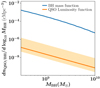 |
Fig. 7. Mass function of active black holes at z ∼ 6.8 computed from the quasar luminosity function (orange), compared to the empirically derived mass function of all black holes at this redshift (blue). The solid orange line represents an Eddington ratio of ηEdd = 0.5 and the shaded region covers the range 0.1 ≤ ηEdd ≤ 1, which is motivated by observations at z ≃ 6. |
The ratio of Eqs. (17) and (18) defines the active fraction of black holes (e.g., Shankar et al. 2013) as a function of their mass:
 (19)
(19)
This value is of the order of 10−4 − 10−5 depending on the assumed mass and Eddington ratio of the black holes. It is provided in the second column of Table 2 for the two masses of the black holes under present consideration and at η = 0.5.
Active quasar fraction as a function of primary black hole mass at a median redshift of z ∼ 6.8 (second column), and total number of quasar counterparts over a redshift interval 6 < z < 7.1 (third column) expected inside the SKA localization ellipse, assuming a logarithmic mass interval of dlog10MBH = 0.1 around its central value.
We can then calculate the number of active quasar counterparts as a function of the black hole separation (or, equivalently, the observed frequency of the gravitational wave event) by combining the quasar luminosity function with the detectable region in Figs. 5 and 6. This is done by computing the following quantity:
 (20)
(20)
where factive and dNBHB, gw are defined in Eqs. (19) and (14), respectively. Figures 8 and 9 show this quantity per unit logarithmic black hole mass interval at z ∼ 6.8, for both the masses of the primary black hole under consideration, as a function of the black hole separation, a (which determines qmin, according to Figs. 5 and 6). In both plots, the comoving volume is taken to be that enclosed between z ∼ 6 and z ∼ 7.1 with a full-sky areal coverage. The near-constant nature of dNQSO/dlog10MBH (with separation) is a consequence of qmin being nearly independent of a (as seen in previous figures). We note, however, that the number of active quasars expected is strongly dependent on their mean Eddington ratio – this is shown by plotting dNQSO/dlog10MBH as a function of ηEdd at a fiducial separation of a = 10 mpc in Fig. 10, for both values of MBH under consideration.
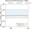 |
Fig. 8. Expected number of active quasars at z ∼ 6.8 over the whole sky as a function of separation, with the primary black hole mass MBH = 109 M⊙. The observed frequency corresponding to the separation is shown on the top axis. |
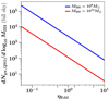 |
Fig. 10. Expected number of active quasar counterparts of SMBH binary mergers with MBH = 109, 1010 M⊙ at z ∼ 6.8 over the whole sky, as a function of the Eddington ratio. The separation in both cases is fixed to a = 10 mpc. |
The preceding analysis thus enables us to connect the number of high-redshift gravitational wave counterparts detected to an important property of the quasar, namely its accretion efficiency. We can now combine these findings with observations of z > 6 quasars in the literature for which mass and Eddington ratio estimates already exist. We use the compilation in Kim & Im (2019), which lists the derived rest-UV and FIR properties of redshift z ≳ 6 quasars. In each case, we calculate the number of expected counterparts within the whole sky area if the system were in a binary. This is tabulated in Table 3 and shown in Fig. 11, which also provides a three-dimensional representation of the results in the previous figure (Fig. 10) and is obtained by gridded interpolation over both the mass and Eddington ratio ranges. The derived i-band magnitudes of the quasars are also shown in Table 3, which can be estimated from the black hole masses and Eddington ratios (Haiman et al. 2009) by adopting a typical quasar spectral energy distribution:
![Mathematical equation: $$ \begin{aligned} m_i = 24 + 2.5 \log \left[\left(\frac{\eta _{\rm Edd}}{0.3}\right) \left(\frac{M_{\rm BH}}{3 \times 10^6\,M_{\odot }}\right)^{-1} \left(\frac{d_{\rm L}(z)}{d_{\rm L}(z = 2)}\right)^2\right] .\end{aligned} $$](/articles/aa/full_html/2023/08/aa45911-23/aa45911-23-eq25.gif) (21)
(21)
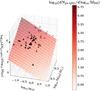 |
Fig. 11. Predicted number of quasar counterparts (in the full sky) for black holes at z ≳ 6, as a joint function of their masses and Eddington ratios. Black holes with known masses and Eddington ratios from the literature (Kim & Im 2019) are indicated by the black triangles superimposed on the figure. |
Predicted number of quasar counterparts and their i-band luminosities for black holes in the literature for which masses and Eddington ratio estimates exist, assuming the system to be in a binary.
A possible source of error in the magnitudes above may arise from the correction to dL induced by weak lensing of the GWs through the large-scale inhomogeneities along their path (Hirata et al. 2010). Assuming this correction to be given by the fitting form introduced in that work, it is expected to lead to about a 10–20% error in the inferred magnitude3. Another contribution to the uncertainty stems from the redshift determination of the source, which we assume to be negligible for the present purposes, as it has been determined by an independent high-resolution measurement (such as the UV/FIR surveys used for the results given in Table 3).
The above arguments can also be reversed to place constraints on the active lifetime of quasars at these redshifts. This is done by not assuming an observationally determined quasar luminosity function as above, but instead, defining the expected active fraction in terms of the mean age of the quasars as:
 (22)
(22)
where tH is the Hubble time at the redshift under consideration. Using this for factive in Eq. (20), we plot the number of expected quasar counterparts as a function of the quasar age (in units of the Hubble time) in Fig. 12 (with qmin assumed to be {0.25, 0.005} for the primary black hole mass MBH = {109, 1010} M⊙, respectively).
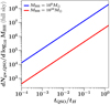 |
Fig. 12. Expected number of active quasar counterparts with MBH = 109, 1010 M⊙ at z ∼ 6.8 over the whole sky, as a function of the mean quasar age (expressed in terms of the Hubble time tH). |
The above results can be converted into the number of active quasar counterparts within a sky area, as a function of the active lifetime of the quasar. This is shown for an area within the SKA localization ellipse of 70 deg2 in the third column of Table 2. It is found that the number of active quasar counterparts of 109 M⊙ black holes (in a logarithmic mass interval of dlog10MBH = 0.1) within the SKA localization ellipse is Ngw, QSO = 7 − 45, and that for 1010 M⊙ black holes is ≲1 (Ngw, QSO = 0.1 − 1.2) for Eddington ratios in the range ηEdd = {0.1, 1}. This (as well as the findings of Table 3) indicate that the quasar counterparts of the most massive black holes at z ≳ 6 can be uniquely identified within the SKA localization ellipse.
4. Discussion
We have investigated the ability of SKA PTA to locate and identify SMBH binaries at z ≳ 6. We find that SKA PTA should be sensitive to black hole binaries with primary masses MBH ≳ 109 M⊙ at all redshifts. The minimum mass ratio constrainable by the SKA varies from ∼0.005 to 0.25, as MBH goes from 109 M⊙ to 1010 M⊙, fairly independently of separation. At z > 6, the regime of SKA PTA detectability covers binary separations of about ∼1 − 50 mpc, depending on the mass of the primary black hole. Binaries with such separations are expected to be close to final coalescence (Begelman et al. 1980; Graham et al. 2015) with their orbital timescales of the order of a few weeks to years.
For the values of the black hole masses and separations considered here, the gravitational wave decay timescale at the radius, agr, is of the order of 100 Myr, consistently with the results of simulations and analytical models (Tiede et al. 2020; Loeb 2007; Nasim et al. 2020; Bogdanović et al. 2022). We have assumed, following previous work (Padmanabhan & Loeb 2020) that the mergers rapidly proceed to coalescence. For small mass ratio mergers, it has been postulated that the dynamical friction timescale could be larger than the Hubble time (Callegari et al. 2011), leading to the so-called “final parsec problem” (Yu 2002; Milosavljević & Merritt 2001). From observations of smaller-mass black hole binaries (Fishbach & Kalogera 2021) at lower redshifts, this delay has been estimated as a function of parameters, such as the progenitor mass and metallicity, finding most binaries to have low delay times of < 500 Myr. This value is likely to be further reduced as the masses of the black holes become higher. There is also observational evidence from X-shaped radio sources (Dennett-Thorpe et al. 2002) favoring efficient binary coalescence (Merritt & Ekers 2002) that can, in turn, result from a number of processes, such as non-spherical galaxy shapes leading to filled loss cones, or gas-rich environments (Haiman et al. 2009; Armitage & Natarajan 2002; Colpi 2014). We leave a more detailed consideration of these effects to future work.
Using empirically motivated constraints on the occupation of black holes in dark matter halos, we find that the number of gravitational wave sources detectable by SKA PTA is about 105 − 106 at z ≳ 6. With their orbital velocities approaching 0.2c, a host of techniques including relativistic Doppler boosting leading to periodic variability in the optical light curves can be used to identify the electromagnetic counterparts of detected gravitational wave events.
Using currently available constraints on the black hole mass-circular velocity relation at high redshifts, combined with the latest observations of the quasar luminosity function at z > 6, we predicted the expected number of active quasar counterparts to SKA PTA detections, finding that the electromagnetic counterparts of the most massive black holes at z ∼ 6 should be uniquely identifiable in the SKA localization ellipse. In so doing, we also developed data-driven estimates for the number of active quasar counterparts to the PTA events, as a function of the quasar’s Eddington luminosity and active lifetime – two parameters that are directly related to the black hole growth mechanism (Farina et al. 2022). This allowed us to derive the expected numbers of quasar counterparts of known black holes at z ≳ 6 if the system were to be in a binary. Our results imply that identifying the counterparts of PTA events with the SKA will offer the possibility to place robust constraints on the seeding and growth mechanisms of high-z SMBHs.
While the term “quasar” has traditionally been used to describe radio-loud quasi-stellar objects, we use the terms “QSOs” and “quasars” interchangeably throughout this work, irrespective of their radio properties.
More exotic sources include cosmic strings (Siemens et al. 2007; Blanco-Pillado et al. 2018; Damour & Vilenkin 2001), phase transitions (Caprini 2010; Kobakhidze et al. 2017) or a primordial GW background in the early Universe (Grishchuk 2005; Lasky et al. 2016).
While the said fitting form is calibrated until z ∼ 3, for the purposes of this discussion, we assume it to be valid out to z ∼ 6.
Acknowledgments
HP’s research is supported by the Swiss National Science Foundation via Ambizione Grant PZ00P2_179934. The work of AL is supported in part by the Black Hole Initiative, which is funded by grants from the John Templeton Foundation and the Gordon and Betty Moore Foundation. We thank the referee for a helpful report.
References
- Agarwal, B., Smith, B., Glover, S., Natarajan, P., & Khochfar, S. 2016, MNRAS, 459, 4209 [NASA ADS] [CrossRef] [Google Scholar]
- Armitage, P. J., & Natarajan, P. 2002, ApJ, 567, L9 [NASA ADS] [CrossRef] [Google Scholar]
- Bañados, E., Venemans, B. P., Mazzucchelli, C., et al. 2018, Nature, 553, 473 [Google Scholar]
- Barkana, R., & Loeb, A. 2001, Phys. Rep., 349, 125 [NASA ADS] [CrossRef] [Google Scholar]
- Begelman, M. C., Blandford, R. D., & Rees, M. J. 1980, Nature, 287, 307 [Google Scholar]
- Blanco-Pillado, J. J., Olum, K. D., & Siemens, X. 2018, Phys. Lett. B, 778, 392 [NASA ADS] [CrossRef] [Google Scholar]
- Bogdanović, T., Bode, T., Haas, R., Laguna, P., & Shoemaker, D. 2011, Class. Quant. Grav., 28, 094020 [CrossRef] [Google Scholar]
- Bogdanović, T., Miller, M. C., & Blecha, L. 2022, Liv. Rev. Relat., 25, 3 [Google Scholar]
- Bonetti, M., Sesana, A., Barausse, E., & Haardt, F. 2018, MNRAS, 477, 2599 [NASA ADS] [CrossRef] [Google Scholar]
- Bonoli, S., Mayer, L., & Callegari, S. 2014, MNRAS, 437, 1576 [NASA ADS] [CrossRef] [Google Scholar]
- Bouwens, R. J., Illingworth, G. D., Blakeslee, J. P., & Franx, M. 2006, ApJ, 653, 53 [NASA ADS] [CrossRef] [Google Scholar]
- Bromm, V., & Loeb, A. 2003, ApJ, 596, 34 [Google Scholar]
- Burke-Spolaor, S., Taylor, S. R., Charisi, M., et al. 2019, A&ARv, 27, 5 [Google Scholar]
- Callegari, S., Kazantzidis, S., Mayer, L., et al. 2011, ApJ, 729, 85 [NASA ADS] [CrossRef] [Google Scholar]
- Caprini, C. 2010, ArXiv e-prints [arXiv:1005.5291] [Google Scholar]
- Carr, B. J., & Hawking, S. W. 1974, MNRAS, 168, 399 [NASA ADS] [CrossRef] [Google Scholar]
- Casey-Clyde, J. A., Mingarelli, C. M. F., Greene, J. E., et al. 2022, ApJ, 924, 93 [NASA ADS] [CrossRef] [Google Scholar]
- Charisi, M., Bartos, I., Haiman, Z., et al. 2016, MNRAS, 463, 2145 [Google Scholar]
- Colpi, M. 2014, Space Sci. Rev., 183, 189 [Google Scholar]
- Cordes, J., Kramer, M., Lazio, T., et al. 2004, New Astron. Rev., 48, 1413 [CrossRef] [Google Scholar]
- Damour, T., & Vilenkin, A. 2001, Phys. Rev. D, 64, 064008 [NASA ADS] [CrossRef] [Google Scholar]
- Dennett-Thorpe, J., Scheuer, P. A. G., Laing, R. A., et al. 2002, MNRAS, 330, 609 [NASA ADS] [CrossRef] [Google Scholar]
- De Rosa, G., Venemans, B. P., Decarli, R., et al. 2014, ApJ, 790, 145 [Google Scholar]
- D’Orazio, D. J., & Di Stefano, R. 2018, MNRAS, 474, 2975 [CrossRef] [Google Scholar]
- D’Orazio, D. J., Haiman, Z., & MacFadyen, A. 2013, MNRAS, 436, 2997 [Google Scholar]
- D’Orazio, D. J., Haiman, Z., Duffell, P., Farris, B. D., & MacFadyen, A. I. 2015a, MNRAS, 452, 2540 [CrossRef] [Google Scholar]
- D’Orazio, D. J., Haiman, Z., & Schiminovich, D. 2015b, Nature, 525, 351 [Google Scholar]
- Eilers, A.-C., Hennawi, J. F., Decarli, R., et al. 2020, ApJ, 900, 37 [Google Scholar]
- Eilers, A.-C., Hennawi, J. F., Davies, F. B., & Simcoe, R. A. 2021, ApJ, 917, 38 [NASA ADS] [CrossRef] [Google Scholar]
- Fakhouri, O., Ma, C.-P., & Boylan-Kolchin, M. 2010, MNRAS, 406, 2267 [Google Scholar]
- Fan, X., Strauss, M. A., Richards, G. T., et al. 2006, AJ, 131, 1203 [NASA ADS] [CrossRef] [Google Scholar]
- Fang, Y., & Yang, H. 2023, MNRAS, 523, 5120 [NASA ADS] [CrossRef] [Google Scholar]
- Farina, E. P., Schindler, J.-T., Walter, F., et al. 2022, ApJ, 941, 106 [NASA ADS] [CrossRef] [Google Scholar]
- Feng, Y., Li, D., Zheng, Z., & Tsai, C.-W. 2020, Phys. Rev. D, 102, 023014 [NASA ADS] [CrossRef] [Google Scholar]
- Feruglio, C., Fiore, F., Carniani, S., et al. 2018, A&A, 619, A39 [NASA ADS] [CrossRef] [EDP Sciences] [Google Scholar]
- Fishbach, M., & Kalogera, V. 2021, ApJ, 914, L30 [CrossRef] [Google Scholar]
- Flesch, E. W. 2021, ArXiv e-prints [arXiv:2105.12985] [Google Scholar]
- Gallo, E., & Sesana, A. 2019, ApJ, 883, L18 [NASA ADS] [CrossRef] [Google Scholar]
- Garcia-Bellido, J., Murayama, H., & White, G. 2021, J. Cosmol. Astropart. Phys., 2021, 023 [CrossRef] [Google Scholar]
- Graham, M. J., Djorgovski, S. G., Stern, D., et al. 2015, Nature, 518, 74 [Google Scholar]
- Grishchuk, L. P. 2005, Physics-Uspekhi, 48, 1235 [NASA ADS] [CrossRef] [Google Scholar]
- Haehnelt, M. G., & Rees, M. J. 1993, MNRAS, 263, 168 [Google Scholar]
- Haiman, Z. 2017, Phys. Rev. D, 96, 023004 [NASA ADS] [CrossRef] [Google Scholar]
- Haiman, Z., & Loeb, A. 2001, ApJ, 552, 459 [NASA ADS] [CrossRef] [Google Scholar]
- Haiman, Z., Kocsis, B., & Menou, K. 2009, ApJ, 700, 1952 [CrossRef] [Google Scholar]
- Hayasaki, K., & Loeb, A. 2016, Sci. Rep., 6, 35629 [NASA ADS] [CrossRef] [Google Scholar]
- Hirata, C. M., Holz, D. E., & Cutler, C. 2010, Phys. Rev. D, 81, 124046 [NASA ADS] [CrossRef] [Google Scholar]
- Inayoshi, K., & Haiman, Z. 2016, ApJ, 828, 110 [CrossRef] [Google Scholar]
- Inayoshi, K., Visbal, E., & Haiman, Z. 2020, ARA&A, 58, 27 [NASA ADS] [CrossRef] [Google Scholar]
- Janssen, G., Hobbs, G., McLaughlin, M., et al. 2015, Advancing Astrophysics with the Square Kilometre Array (AASKA14), 37 [Google Scholar]
- Kaiser, A. R., Pol, N. S., McLaughlin, M. A., et al. 2022, ApJ, 938, 115 [NASA ADS] [CrossRef] [Google Scholar]
- Khrykin, I. S., Hennawi, J. F., Worseck, G., & Davies, F. B. 2021, MNRAS, 505, 649 [CrossRef] [Google Scholar]
- Kim, Y., & Im, M. 2019, ApJ, 879, 117 [NASA ADS] [CrossRef] [Google Scholar]
- King, A. 2016, MNRAS, 456, L109 [CrossRef] [Google Scholar]
- Kobakhidze, A., Lagger, C., Manning, A., & Yue, J. 2017, Eur. Phys. J. C, 77, 570 [NASA ADS] [CrossRef] [Google Scholar]
- Kocsis, B., Frei, Z., Haiman, Z., & Menou, K. 2006, ApJ, 637, 27 [NASA ADS] [CrossRef] [Google Scholar]
- Kramer, M. 2004, New Astron. Rev., 48, 1413 [CrossRef] [Google Scholar]
- Kulkarni, G., & Loeb, A. 2012, MNRAS, 422, 1306 [NASA ADS] [CrossRef] [Google Scholar]
- Lasky, P. D., Mingarelli, C. M. F., Smith, T. L., et al. 2016, Phys. Rev. X, 6, 011035 [NASA ADS] [Google Scholar]
- Liu, K., Verbiest, J. P. W., Kramer, M., et al. 2011, MNRAS, 417, 2916 [Google Scholar]
- Lodato, G., & Natarajan, P. 2006, MNRAS, 371, 1813 [NASA ADS] [CrossRef] [Google Scholar]
- Lodato, G., & Natarajan, P. 2007, MNRAS, 377, L64 [NASA ADS] [Google Scholar]
- Loeb, A. 2007, Phys. Rev. Lett., 99, 041103 [NASA ADS] [CrossRef] [Google Scholar]
- Loeb, A. 2010, Phys. Rev. D, 81, 047503 [NASA ADS] [CrossRef] [Google Scholar]
- LSST Science Collaboration (Abell, P. A., et al.) 2009, ArXiv e-prints [arXiv:0912.0201] [Google Scholar]
- Lusso, E., Valiante, R., & Vito, F. 2023, in Handbook of X-ray and Gamma-ray Astrophysics, eds. C. Bambi & A. Santangelo (Springer Living Reference Work), 122 [Google Scholar]
- Madau, P., & Rees, M. J. 2001, ApJ, 551, L27 [Google Scholar]
- Maiorano, M., De Paolis, F., & Nucita, A. A. 2021, Symmetry, 13, 2418 [NASA ADS] [CrossRef] [Google Scholar]
- Merritt, D. 2000, ASP Conf. Ser., 197, 221 [NASA ADS] [Google Scholar]
- Merritt, D., & Ekers, R. D. 2002, Science, 297, 1310 [NASA ADS] [CrossRef] [Google Scholar]
- Millon, M., Dalang, C., Lemon, C., et al. 2022, A&A, 668, A77 [NASA ADS] [CrossRef] [EDP Sciences] [Google Scholar]
- Milosavljević, M., & Merritt, D. 2001, ApJ, 563, 34 [Google Scholar]
- Milosavljević, M., & Merritt, D. 2003, AIP Conf. Ser., 686, 201 [CrossRef] [Google Scholar]
- Moore, C. J., Cole, R. H., & Berry, C. P. L. 2015, Class. Quant. Grav., 32, 015014 [NASA ADS] [CrossRef] [Google Scholar]
- Mortlock, D. J., Warren, S. J., Venemans, B. P., et al. 2011, Nature, 474, 616 [Google Scholar]
- Nasim, I., Gualandris, A., Read, J., et al. 2020, MNRAS, 497, 739 [Google Scholar]
- Natarajan, P., & Treister, E. 2009, MNRAS, 393, 838 [NASA ADS] [CrossRef] [Google Scholar]
- Natarajan, P., Pacucci, F., Ferrara, A., et al. 2017, ApJ, 838, 117 [NASA ADS] [CrossRef] [Google Scholar]
- Nobuta, K., Akiyama, M., Ueda, Y., et al. 2012, ApJ, 761, 143 [NASA ADS] [CrossRef] [Google Scholar]
- Onoue, M., Kashikawa, N., Matsuoka, Y., et al. 2019, ApJ, 880, 77 [Google Scholar]
- Pacucci, F., & Loeb, A. 2022, MNRAS, 509, 1885 [Google Scholar]
- Pacucci, F., Natarajan, P., Volonteri, M., Cappelluti, N., & Urry, C. M. 2017, ApJ, 850, L42 [NASA ADS] [CrossRef] [Google Scholar]
- Padmanabhan, H., & Loeb, A. 2020, J. Cosmol. Astropart. Phys., 2020, 055 [CrossRef] [Google Scholar]
- Peters, P. C. 1964, Phys. Rev., 136, 1224 [Google Scholar]
- Pol, N. S., Taylor, S. R., Kelley, L. Z., et al. 2021, ApJ, 911, L34 [NASA ADS] [CrossRef] [Google Scholar]
- Rajagopal, M., & Romani, R. W. 1995, ApJ, 446, 543 [NASA ADS] [CrossRef] [Google Scholar]
- Rees, M. J. 1984, ARA&A, 22, 471 [Google Scholar]
- Ricarte, A., & Natarajan, P. 2018, MNRAS, 481, 3278 [NASA ADS] [CrossRef] [Google Scholar]
- Rosado, P. A., Sesana, A., & Gair, J. 2015, MNRAS, 451, 2417 [NASA ADS] [CrossRef] [Google Scholar]
- Rosado, P. A., Lasky, P. D., Thrane, E., et al. 2016, Phys. Rev. Lett., 116, 101102 [NASA ADS] [CrossRef] [Google Scholar]
- Salpeter, E. E. 1964, ApJ, 140, 796 [NASA ADS] [CrossRef] [Google Scholar]
- Sesana, A., Haardt, F., Madau, P., & Volonteri, M. 2004, ApJ, 611, 623 [NASA ADS] [CrossRef] [Google Scholar]
- Shankar, F., Weinberg, D. H., & Miralda-Escudé, J. 2013, MNRAS, 428, 421 [NASA ADS] [CrossRef] [Google Scholar]
- Shen, X., Hopkins, P. F., Faucher-Giguère, C.-A., et al. 2020, MNRAS, 495, 3252 [Google Scholar]
- Sheth, R. K., & Tormen, G. 2002, MNRAS, 329, 61 [Google Scholar]
- Siemens, X., Mandic, V., & Creighton, J. 2007, Phys. Rev. Lett., 98, 111101 [NASA ADS] [CrossRef] [Google Scholar]
- Smits, R., Kramer, M., Stappers, B., et al. 2009, A&A, 493, 1161 [NASA ADS] [CrossRef] [EDP Sciences] [Google Scholar]
- Spallicci, A. D. A. M. 2013, ApJ, 764, 187 [NASA ADS] [CrossRef] [Google Scholar]
- Stappers, B. W., Keane, E. F., Kramer, M., Possenti, A., & Stairs, I. H. 2018, Phil. Trans. R. Soc. London Ser. A, 376, 20170293 [Google Scholar]
- Taylor, S. R., Vallisneri, M., Ellis, J. A., et al. 2016, ApJ, 819, L6 [NASA ADS] [CrossRef] [Google Scholar]
- Tiede, C., Zrake, J., MacFadyen, A., & Haiman, Z. 2020, ApJ, 900, 43 [NASA ADS] [CrossRef] [Google Scholar]
- Trakhtenbrot, B., Lira, P., Netzer, H., et al. 2017, Front. Astron. Space Sci., 4 [Google Scholar]
- Tremaine, S., Gebhardt, K., Bender, R., et al. 2002, ApJ, 574, 740 [NASA ADS] [CrossRef] [Google Scholar]
- Turner, E. L. 1991, AJ, 101, 5 [NASA ADS] [CrossRef] [Google Scholar]
- Valtonen, M. J., Zola, S., Ciprini, S., et al. 2016, ApJ, 819, L37 [NASA ADS] [CrossRef] [Google Scholar]
- Venemans, B. P., Walter, F., Zschaechner, L., et al. 2016, ApJ, 816, 37 [Google Scholar]
- Venemans, B. P., Walter, F., Decarli, R., et al. 2017, ApJ, 851, L8 [NASA ADS] [CrossRef] [Google Scholar]
- Verbiest, J. P. W., Lentati, L., Hobbs, G., et al. 2016, MNRAS, 458, 1267 [Google Scholar]
- Volonteri, M. 2010, A&ARv, 18, 279 [Google Scholar]
- Volonteri, M. 2012, Science, 337, 544 [NASA ADS] [CrossRef] [Google Scholar]
- Wang, Y., & Mohanty, S. D. 2017, Phys. Rev. Lett., 118, 151104 [NASA ADS] [CrossRef] [Google Scholar]
- Wei, D., Cheng, C., Zheng, Z., & Hong, W. 2020, AJ, 159, 138 [CrossRef] [Google Scholar]
- Wen, Z. L., Jenet, F. A., Yardley, D., Hobbs, G. B., & Manchester, R. N. 2011, ApJ, 730, 29 [NASA ADS] [CrossRef] [Google Scholar]
- Westernacher-Schneider, J. R., Zrake, J., MacFadyen, A., & Haiman, Z. 2022, Phys. Rev. D, 106, 103010 [NASA ADS] [CrossRef] [Google Scholar]
- Willott, C. J., Carilli, C. L., Wagg, J., & Wang, R. 2015, ApJ, 807, 180 [NASA ADS] [CrossRef] [Google Scholar]
- Wu, X.-B., Wang, F., Fan, X., et al. 2015, Nature, 518, 512 [Google Scholar]
- Wyithe, J. S. B., & Loeb, A. 2002, ApJ, 581, 886 [NASA ADS] [CrossRef] [Google Scholar]
- Xin, C., & Haiman, Z. 2021, MNRAS, 506, 2408 [NASA ADS] [CrossRef] [Google Scholar]
- Yu, Q. 2002, MNRAS, 331, 935 [Google Scholar]
All Tables
Expected numbers of black hole binaries detectable by the SKA PTA at the median redshift of z ∼ 6.8, along with their galaxy counterparts, detectable by LSST.
Active quasar fraction as a function of primary black hole mass at a median redshift of z ∼ 6.8 (second column), and total number of quasar counterparts over a redshift interval 6 < z < 7.1 (third column) expected inside the SKA localization ellipse, assuming a logarithmic mass interval of dlog10MBH = 0.1 around its central value.
Predicted number of quasar counterparts and their i-band luminosities for black holes in the literature for which masses and Eddington ratio estimates exist, assuming the system to be in a binary.
All Figures
|
Fig. 1. Distribution of estimated black hole masses in observed z > 6 quasars. Masses are derived from bolometric luminosities (when available), assuming Eddington ratios from Nobuta et al. (2012). These are also consistent with mass estimates derived independently in the literature. |
| In the text | |
|
Fig. 2. Strain vs. observed frequency of SKA PTA (blue curve, from Garcia-Bellido et al. 2021). The red dots mark example points on the trajectory of a binary system at z ∼ 6.8 with masses of M1 = 1010 M⊙ and M2 ≈ 3 × 10⁷ M⊙ as a function of the gravitational wave decay timescale, tGW, measured in units of years in the observer’s frame of reference. |
| In the text | |
|
Fig. 3. Constraints on the q − a plane from the SKA sensitivity curve and assuming a primary black hole mass M1 = 109 M⊙ at various redshifts. The dashed line shows the innermost stable circular orbit (ISCO). |
| In the text | |
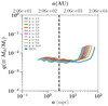 |
Fig. 4. Same as Fig. 3, but for the primary black hole mass, M1 = 1010 M⊙. |
| In the text | |
|
Fig. 5. Constraints on the q − a plane from the SKA sensitivity curve and assuming a primary black hole mass M1 = 109 M⊙ at z ∼ 6.8. The dashed line shows the innermost stable circular orbit (ISCO), while the shaded region indicates the regime of detectability of the binary SMBH with SKA PTA The top axes show the observed gravitational wave decay time and the orbital period of the binary and the velocity of the lower-mass black hole. The range of velocities in the regime of detectability is of the order of 0.06c − 0.2c, ensuring good prospects for prompt electromagnetic follow-ups via Doppler boosting of the light curves. |
| In the text | |
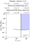 |
Fig. 6. Same as Fig. 5, for a primary black hole of mass of M1 = 1010 M⊙ at z ∼ 6.8. |
| In the text | |
|
Fig. 7. Mass function of active black holes at z ∼ 6.8 computed from the quasar luminosity function (orange), compared to the empirically derived mass function of all black holes at this redshift (blue). The solid orange line represents an Eddington ratio of ηEdd = 0.5 and the shaded region covers the range 0.1 ≤ ηEdd ≤ 1, which is motivated by observations at z ≃ 6. |
| In the text | |
|
Fig. 8. Expected number of active quasars at z ∼ 6.8 over the whole sky as a function of separation, with the primary black hole mass MBH = 109 M⊙. The observed frequency corresponding to the separation is shown on the top axis. |
| In the text | |
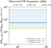 |
Fig. 9. Same as Fig. 8, for a primary black hole of the mass MBH = 1010 M⊙. |
| In the text | |
|
Fig. 10. Expected number of active quasar counterparts of SMBH binary mergers with MBH = 109, 1010 M⊙ at z ∼ 6.8 over the whole sky, as a function of the Eddington ratio. The separation in both cases is fixed to a = 10 mpc. |
| In the text | |
|
Fig. 11. Predicted number of quasar counterparts (in the full sky) for black holes at z ≳ 6, as a joint function of their masses and Eddington ratios. Black holes with known masses and Eddington ratios from the literature (Kim & Im 2019) are indicated by the black triangles superimposed on the figure. |
| In the text | |
|
Fig. 12. Expected number of active quasar counterparts with MBH = 109, 1010 M⊙ at z ∼ 6.8 over the whole sky, as a function of the mean quasar age (expressed in terms of the Hubble time tH). |
| In the text | |
Current usage metrics show cumulative count of Article Views (full-text article views including HTML views, PDF and ePub downloads, according to the available data) and Abstracts Views on Vision4Press platform.
Data correspond to usage on the plateform after 2015. The current usage metrics is available 48-96 hours after online publication and is updated daily on week days.
Initial download of the metrics may take a while.