| Issue |
A&A
Volume 663, July 2022
|
|
|---|---|---|
| Article Number | A153 | |
| Number of page(s) | 26 | |
| Section | Extragalactic astronomy | |
| DOI | https://doi.org/10.1051/0004-6361/202039750 | |
| Published online | 27 July 2022 | |
What is the origin of the stacked radio emission in radio-undetected quasars?
Insights from a radio-infrared image stacking analysis
1
Leiden Observatory, Leiden University, PO Box 9513 Leiden 2300 RA, The Netherlands
e-mail: This email address is being protected from spambots. You need JavaScript enabled to view it.
2
Astrophysics and Cosmology Research Unit, School of Mathematics, Statistics and Computer Science, University of KwaZulu-Natal, Durban 4041, South Africa
Received:
23
October
2020
Accepted:
30
November
2021
Abstract
Radio emission in the brightest radio quasars can be attributed to processes inherent to active galactic nuclei (AGN) powered by super massive black holes (SMBHs), while the physical origins of the radio fluxes in quasars without radio detections have not been established with full certainly. Deep radio surveys carried out with the Low Frequency ARray (LOFAR) are at least one order of magnitude more sensitive for objects with typical synchrotron spectra than previous wide-area high-frequency surveys ( > 1.0 GHz). With the enhanced sensitivity that LOFAR offers, we investigate the radio-infrared continuum of LOFAR radio-detected quasars (RDQs) and LOFAR radio-undetected quasars (RUQs) in the 9.3 deg2 NOAO Deep Wide-field survey (NDWFS) of the Boötes field; RUQs are quasars that are individually undetected at a level of ≥5σ in the LOFAR observations. To probe the nature of the radio and infrared emission, where direct detection is not possible due to the flux density limits, we used a median image stacking procedure. This was done in the radio frequencies of 150 MHz, 325 MHz, 1.4 GHz and 3.0 GHz, and in nine infrared bands between 8 and 500 μm. The stacking analysis allows us to probe the radio-luminosity for quasars that are up to one order of magnitude fainter than the ones detected directly. The radio and infrared photometry allow us to derive the median spectral energy distributions of RDQs and RUQs in four contiguous redshift bins between 0 < z < 6.15. The infrared photometry is used to derive the infrared star-formation rate (SFR) through SED fitting, and is compared with two independent radio-based star-formation (SF) tracers using the far-infrared radio correlation (FIRC) of star-forming galaxies. We find a good agreement between our radio and infrared SFR measurements and the predictions of the FIRC. Moreover, we use the FIRC predictions to establish the level of the contribution due to SMBH accretion to the total radio-luminosity. We show that SMBH accretion can account for ∼5−41% of the total radio-luminosity in median RUQs, while for median RDQs the contribution is ∼50−84%. This implies that vigorous SF activity is coeval with SMBH growth in our median stacked quasars. We find that median RDQs have higher SFRs that agree well with those of massive star-forming main sequence galaxies, while median RUQs present lower SFRs than RDQs. Furthermore, the behavior of the radio-loudness parameter (R = log10(Lrad/LAGN)) is investigated. For quasars with R ≥ −4.5, the radio-emission is consistent with being dominated by SMBH accretion, while for low radio luminosity quasars with R < −4.5 the relative contribution of SF to the radio fluxes increases as the SMBH component becomes weaker. We also find signatures of SF suppression due to negative AGN feedback in the brightest median RDQs at 150 MHz. Finally, taking advantage of our broad spectral coverage, we studied the radio spectra of median RDQs and RUQs. The spectral indices of RUQs and RDQs do not evolve significantly with redshift, but they become flatter towards lower frequencies.
Key words: quasars: general / quasars: supermassive black holes / radio continuum: galaxies / radio continuum: general
© ESO 2022
1. Introduction
Even though more than five decades have passed since the discovery of the first radio quasar by Schmidt (1963), the physical processes responsible for the radio emission in quasars are not fully understood. The radio emission in the brightest radio quasars, known as radio-loud quasars (RLQs), is associated with the accretion onto supermassive black holes (SMBHs). The accretion energy output often manifests as large-scale structures (radio jets and lobes). The origins of the weaker radio emission in the fainter radio quasars, called radio-quiet quasars (RQQs), are still uncertain. It has been suggested that the radio activity in RQQs is produced by a starburst. It is thought that the starburst radio-emission has a synchrotronic component produced by electrons accelerated by supernovae remnants, and a thermal free-free component arising from the ionization of hydrogen clouds (HII regions) by hot massive stars (Sopp & Alexander 1991; Terlevich & Boyle 1993). Conversely, it had been proposed that the radio emission in RQQs is caused by small-scale radio jets with a kinetic power that is significantly lower ( ∼ 1000) than those of RLQs (Miller et al. 1993). This scenario is supported by high-resolution observations of RQQs, where the brightness temperatures and jet-like structure of the radio emission suggest that the radio emission in RQQs has a non-thermal origin (Blundell et al. 1996; Ulvestad et al. 2005; Leipski et al. 2006; Herrera Ruiz et al. 2016). Finally, in recent years the possibility that the radio emission in RQQs is driven by magnetically heated accretion disk coronae (Laor & Behar 2008; Laor et al. 2019) and winds from active galactic nuclei (AGN) (Zakamska & Greene 2014; Zakamska et al. 2016; Hwang et al. 2018) has been explored.
The stacking technique combines the signal of many individual sources that have been previously identified in other wavelength observations, some of these sources may be below the noise level (and therefore have gone undetected) in a particular survey. The co-addition brings down the statistical noise, enabling statistical flux measurements of sources below the original detection threshold. Radio image stacking has previously been carried out to study quasars that remain silent in flux density limited surveys due to their low radio power. For example, White et al. (2007) analyzed the stacked FIRST 1.4 GHz radio images of ∼41 000 RQQs positions from the SDSS DR3 survey (Schneider et al. 2005) with 0 < z < 5, which resulted in a median flux density of 110 μJy. Wals et al. (2005) co-added FIRST images of 8000 RQQs of the 2QZ survey (Croom et al. 2004), and found median fluxes of 20−40 μJy. Hwang et al. (2018) found similar flux values by stacking VLA maps of red quasars at 1.4 GHz and 6.0 GHz. White et al. (2015) using a stacking analysis of photometrically and spectroscopically selected quasars with 0 < z < 3.1 in the VISTA Deep Extragalactic Observations (VIDEO, Jarvis et al. 2013) survey found that the radio emission of the quasars in their sample is likely caused by accretion activity. Finally, Perger et al. (2019) found a 1.4 GHz flux density of 52 μJy for 2229 RQQs with 4.0 < z < 7.5 using FIRST radio maps.
An important point to consider in the study of the radio emission of RQQs is the observed frequency. Most of the radio stacking analyses of RQQs have been carried out using high-frequency observations ( > 1.0 GHz). With new low-frequency radio interferometer arrays such as the Low Frequency Array (LOFAR; van Haarlem et al. 2013), we are able to investigate the radio emission of RQQs at very low-frequencies exploring a new parameter space. A number of quasar studies using LOFAR observations have been done in the last few years. For instance, Gürkan et al. (2019) found that the radio emission at 150 MHz in low-luminosity quasars is consistent with being dominated by star formation (SF). Morabito et al. (2019) studied the low-frequency radio properties of broad absorption line quasars. Retana-Montenegro & Röttgering (2018) investigated the selection of high-z quasars using LOFAR observations. Retana-Montenegro & Röttgering (2020) investigated the optical luminosity function of LOFAR radio-selected quasars (RSQs) at 1.4 < z < 5.0 in the NDWFS-Boötes field using deep LOFAR observations of the NDWFS-Boötes field (Retana-Montenegro et al. 2018). They found that RSQs show an evolution that is very similar to the exhibited by faint quasars (M1450 ≤ −22), and that RSQs may compose up to ∼20% of the whole faint quasar population.
Another point of intense study in quasars is to understand the physical origin of the difference between RLQs and RQQs. For this purpose, the radio-loudness parameter, defined as the ratio of radio to optical quantities (fluxes or luminosities), was introduced to classify quasars as radio-loud or radio-quiet (e.g., Kellermann et al. 1989; Ivezić et al. 2002). Across the literature, there is no clear consensus on the radio-loudness limit for classifying quasars. Moreover, the calculation of the ratio depends on the radio and optical bands available, and these bands tend to vary between the studies. This has led to discrepancies between the radio-loudness studies: some authors found that radio-loudness distribution for optical-selected quasars is bimodal (Miller et al. 1990; Jiang et al. 2007; White et al. 2007), while others have confirmed a very broad range for the radio-loudness parameter, and question its bimodal nature (Cirasuolo et al. 2003; Singal et al. 2011; Baloković et al. 2012). In particular, recent LOFAR studies have found that the radio properties of quasars show a continuous distribution rather than a bimodal distribution (Gürkan et al. 2019; Fawcett et al. 2020).
The study of the radio emission in quasars is particularly important for understanding the role of AGN feedback in suppressing or, alternatively, enhancing of SF. The hosts of luminous quasars (LX > 1044 erg s−1) at z > 1 are known to be sites of intense SF (Harris et al. 2016; Pitchford et al. 2016; Dong & Wu 2016; Duras et al. 2017), however, these studies contain an important number of non-detections and are restricted only to objects with the highest star formation rates (SFRs). On the other hand, the results provided by studies of moderate luminosity AGN (Lbol ∼ 1043 − 1044 erg s−1) provide no clear evidence for the AGN influence on the SF of the host galaxy (e.g., Rovilos et al. 2012; Stanley et al. 2015; Azadi et al. 2017). Recent deep observations with ALMA and SCUBA have found that AGN hosts have SFRs lower than those predicted by the SF main sequence (Noeske et al. 2007; Elbaz et al. 2011; Whitaker et al. 2012; Schreiber et al. 2015). This might be an indication for the suppression of SF due to AGN feedback, namely, quenching. The investigation of the properties of radio-detected quasars could provide useful insights of the relationships between SMBHs and the SF on their host galaxies.
In this paper, we use radio and infrared observations of the NDWFS-Boötes field to investigate the origins of the radio emission in LOFAR radio-detected quasars (RDQs) and LOFAR radio-undetected quasars (RUQs). RUQs are defined as quasars that are individually undetected at ≥5σ on the LOFAR map. The NDWFS-Boötes field has a wealth of multi-wavelength datasets with infrared coverage provided by Spitzer, WISE, and Herschel observations along with GMRT, WSRT, and VLA radio imaging at 325 MHz (Coppejans et al. 2015), 1.4 GHz (de Vries et al. 2002), and 3.0 GHz (Lacy et al. 2020), respectively. This is complemented with deep LOFAR observations at 150 MHz (Retana-Montenegro et al. 2018). The key part of our work is that we are using radio maps at low- and high- frequencies that are deep enough to obtain a statistical measurement of the flux densities of RUQs using a stacking analysis. This work will help to address the following questions regarding the radio emission in quasars: (1) is the radio-emission of quasars powered by SF or SMBH accretion?; (2) how similar are the radio spectra indices of RDQs and RUQs?; (3) what is the behaviour of the radio-loudness parameter at low radio luminosities?; (4) can we find signatures of AGN feedback with our data?
This paper is organized as follows. In Sect. 2, we present the data used in this work. In Sect. 3, we introduce our spectroscopic quasar sample, and we discuss our stacking analysis in Sect. 4.1. Section 5 presents the results of our stacking analysis. In Sect. 6, we discuss our findings. Finally, we summarize our conclusions in Sect. 7. Through this paper, we use a Λ cosmology with the matter density Ωm = 0.30, and the cosmological constant ΩΛ = 0.70, the Hubble constant H0 = 70 km s−1 Mpc−1. We assume a definition of the form Sν ∝ ν−α, where Sν is the source flux, ν the observing frequency, and α the spectral index. To estimate the radio luminosities, we adopted a radio spectral index of α = 0.7. The optical luminosities were calculated using a power-law continuum index of ϵopt = 0.5. All the magnitudes are expressed in the AB magnitude system (Oke & Gunn 1983) and are corrected for Galactic extinction using the prescription by Schlafly & Finkbeiner (2011).
2. Data
In this section, we introduce the NDWFS-Boötes datasets that will be utilized in our analysis. A summary of the radio and infrared data used in this work is provided in Table 1.
Summary of the radio and infrared data used in this work.
2.1. Optical data
The NOAO Deep Wide-field survey (NDWFS) is a deep imaging survey in the northern sky (Jannuzi & Dey 1999). A region of 9.3 deg2 towards the Boötes constellation, the Boötes field, was originally observed in the BW, R, and I optical bands, and subsequently imaging in the Uspec (Bian et al. 2013) and ZSubaru bands was obtained. We use the I-band matched photometry catalog presented by Brown et al. (2007). The 5σ limiting AB magnitudes for the optical filters are Uspec = 25.2, Bw = 25.4, R = 25.0, I = 24.9, and ZSubaru = 24.1, respectively. Additionally, the Boötes field has also targeted as part of the observations of the 3π survey performed with the 1.8 m Pan-STARRS1 telescope (Hodapp et al. 2004). The 3π survey (Chambers et al. 2016) observed for almost four years the sky north of −30° declination, reaching 5σ limiting magnitudes in the gPS, rPS, iPS, zPS, yPS bands of 23.3, 23.2, 23.1, 22.3, 21.3, respectively.
2.2. Radio
The NDWFS-Boötes field has been surveyed with various radio-telescopes (e.g., VLA, WSRT, LOFAR) providing an excellent coverage at low- and high- frequencies. The 150 MHz LOFAR observations have been described in Retana-Montenegro et al. (2018). These observations reach a central rms noise of 55 μJy beam−1 with an angular resolution of 3.98″ × 6.45″. The NDWFS-Boötes region was also observed with the VLA in the P-band (VLA-PB) with a central frequency of ∼325 MHz (Coppejans et al. 2015). The VLA-PB mosaic has an angular resolution 5.6″ × 5.1″ with a rms noise of 0.2 mJy beam−1. The NDWFS-Boötes region was also observed with the VLA at 3000 MHz, as part of the VLA Sky Survey (VLASS; Lacy et al. 2020). These observations correspond only to one of the three planned VLASS epochs to be observed. The VLASS mosaic has a resolution of 2.5″ with a sensitivity of 140 μJy beam−1. We also use the 1400 MHz WSRT observations of the NDWFS-Boötes presented by de Vries et al. (2002). The WSRT maps cover approximately 7.0 deg2 of the NDWFS-Boötes field, and have a sensitivity of 28 μJy beam−1 with an angular resolution of 13″ × 27″. Due to the smaller size of the WSRT map, we limit our stacking analysis only to quasars that are located within the footprint of the WSRT-Boötes observations. The footprints of the different radio surveys are shown in Fig. 1.
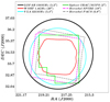 |
Fig. 1. Footprints of the various surveys of the NDWFS-Boötes field used in this work. The beam size for each instrument is also indicated. The 3.0 GHz VLASS observations overlap with the LOFAR region. The analysis in this work is limited to the region with WSRT coverage. |
2.3. Mid-infrared and far-infrared data
The mid-infrared Spitzer Infrared Array Camera (IRAC; Fazio et al. 2004) imaging used in this paper comes from the publicly available images1 from the Spitzer Deep, Wide-field Survey (SDWFS; Ashby et al. 2009) of the NDWFS-Boötes field. The IRAC channels have a field of view of ∼5° and a spatial resolution of 2″. Additionally, we employ Spitzer Multiband Imaging Photometer (MIPS; Rieke et al. 2004) imaging at 24 and 70 μm. At MIPS-24 μm, the resolution is about 6″, and at MIPS-70 μm is about 20″. We retrieved the MIPS data from the Spitzer Heritage Archive2 (Program ID: 50148), and the individual pointings were reduced and mosaiced using the MOPEX package (Makovoz et al. 2006) following a standard calibration (e.g., Sanders et al. 2007). The IRAC-8 μm band reaches a 5σ sensitivity of 30 μJy, while the MIPS data reach depths (1σ) of 51 μJy and 5 mJy, at 24 and 70 μm, respectively. To cover the gap between the IRAC-8 μm and MIPS-24 μm filters, we added to our analysis the WISE-W3 band (Wright et al. 2010) with a central wavelength of λc = 12 μm. We downloaded the WISE-W3 images that cover the WSRT-Boötes region from the IRSA archive3 and created a mosaic using the Montage4 package.
Our far-infrared photometry comes from the Level 6 Herschel Multi-tiered Extragalactic Survey5 (HerMES Oliver et al. 2012). in the NDWFS-Boötes field. HerMES has a 5σ sensitivity of about 25.8, 21.2 and 30.8 mJy at 250, 350 and 500 μm, respectively with the Spectral and Photometric Imaging Receiver (SPIRE; Griffin et al. 2010). The Photodetector Array Camera and Spectrometer (PACS; Poglitsch et al. 2010) has a 5σ sensitivity of 49.9 and 95.1 mJy at 100 and 160 μm. SPIRE provides images having angular resolution ∼18″, 25″ and 37″ at 250, 350 and 500 μm, respectively. The angular resolution of PACS is 6.8″ and 11″ at 100 and 160 μm, respectively. The footprints of the HerMES SPIRE/PACS observations are shown in Fig. 1. We used the HerMES xID24 catalogs, which provide SPIRE and PACS photometry for objects whose positions are taken from catalogs extracted from MIPS-24 μm maps as described by Roseboom et al. (2010).
The far-infrared maps available for NDWFS-Boötes field are shallower in comparison with other extragalactic fields such as COSMOS and GOODs (Oliver et al. 2012). In the 250 μm band, 59% (25%) of the RDQs (RUQs) are detected at ≥3σ, while 92% (78%) are detected with a 2σ significance. To avoid overly complicating the analysis, we set the detection threshold in the SPIRE-250 μm band to 2σ, and classify these quasars as SPIRE-250 μm detected in Sects. 5 and 6, respectively. This threshold allow us to maximize the number of quasars with FIR detections, while simultaneously keeping the number of likely non-detections low.
3. Quasar sample
The starting point to create our sample is the Milliquas catalog from Flesch (2015). This catalog contains all the known NDWFS-Boötes spectroscopic quasars from the literature (e.g., Kochanek et al. 2012; Pâris et al. 2018; Yao et al. 2019). We remark that this catalog is not uniform as it is composed of various surveys with different selection criteria. The majority of quasars in the NDWFS-Boötes sample are type-1, thus, for this reason we use only type-1 spectroscopic quasars in our analysis. We restrict the sample to quasars with positions falling into the WSRT-Boötes footprint. To establish whether a quasar is detected in the radio or not, we use the 150 MHz LOFAR catalog by Retana-Montenegro et al. (2018). We cross-matched both catalogs using a matching radius of 2″, and found that 235 of 1574 quasars are detected at 5σ significance by LOFAR, while 1339 quasars are not detected in the LOFAR maps. From this point, we call the LOFAR detected quasars as radio-detected quasars (RDQs), while LOFAR undetected quasars are denoted as radio-undetected quasars (RUQs). These quasars are not detected individually at ≥5σ in the LOFAR map. We also crossmatch the Milliquas catalog with the WSRT, and VLA 325 Mhz/3.0 GHz catalogs using a matching radius of 15″, 2″, and 1″, respectively. Figure 2 shows the histograms of the quasars detected by each radio telescope. It is clear that the number of quasars detected by LOFAR is significantly larger in comparison with the other radio-telescopes. A total of 21 quasars are detected by WSRT and the VLA, but not by LOFAR. These quasars might not be detected by LOFAR due to having an inverted radio spectra. We omitted the radio flux histogram for these quasars due to their low numbers, but we consider their WSRT/VLA radio fluxes for all our calculations in the rest of the paper. These quasars are undetected by LOFAR, but detected by the other radio-telescopes, therefore according to our requirement, those with a LOFAR 5σ detection are classified as RUQs. The maximum-value normalized I-band magnitude distribution of the quasar samples is presented in Fig. 3. The absolute magnitude and radio luminosity are displayed in Figs. 4 and 5, respectively. The absolute magnitudes at rest-frame 1450 Å, M1450, and K-corrections are calculated following the procedure described by Retana-Montenegro & Röttgering (2020). This is done using the R, I, or ZSubaru band magnitudes depending on the spectroscopic redshift. Figure 6 shows the normalized absolute magnitude M1450 distribution of the quasar samples. The RDQs are slightly brighter than RUQs with a median absolute magnitude of M1450 = −23.0, while RUQs present a median absolute magnitude of M1450 = −22.69.
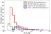 |
Fig. 2. Total flux S150 MHz distributions of LOFAR radio-detected quasars. |
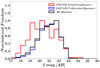 |
Fig. 3. Maximum-value normalized I-band distributions of LOFAR radio-detected quasars (RDQs, red) and LOFAR radio-undetected quasars (RUQs, blue). Also, the total combined redshift distribution of RDQs and RUQs (black) is plotted. |
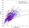 |
Fig. 4. Absolute magnitude at rest-frame 1450 Å, M1450, versus redshift for the LOFAR radio-detected quasars (red) and LOFAR radio-undetected quasars (blue) samples. The dashed line denotes the magnitude limit iPS = 23.0. This limit is calculated assuming a quasar continuum described by a power-law with slope α = −0.5, and with no emission line contribution or Lyα forest blanketing. |
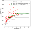 |
Fig. 5. Rest-frame radio luminosity density at 150 MHz versus redshift for LOFAR radio-detected quasars (red) in our sample. The green (LOFAR radio-detected quasars) and gray squares (LOFAR radio-undetected quasars) are the radio luminosities obtained from the stacking analysis in Sect. 4.1. The dashed line denotes the 5σ flux limit (275 μJy) of the NDWFS-Boötes observations presented by Retana-Montenegro et al. (2018). The stacking analysis allows us to probe the radio-luminosity for quasars that are up to one order of magnitude fainter than the ones detected individually. |
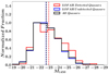 |
Fig. 6. Normalized absolute magnitude M1450 distributions of LOFAR radio-detected quasars (RDQs, red) and LOFAR radio-undetected quasars (RUQs, blue). Also, the combined redshift distribution of RDQs and RUQs (black) is plotted. The median M1450 values of the samples are indicated by the dashed lines. |
4. Methods
4.1. Stacking analysis
The stacking technique permits the extraction of the signal of sources below the detection threshold of a particular survey. We divided our quasar samples into four redshift bins. This allows to have a reasonable number of sources in each bin to achieve a high signal-to-noise ratio (S/N). From the original mosaics, we extracted 50 × 50 pixel cutouts around each quasar position, we also extracted the noise maps. All the cutouts in the redshift bin are grouped together to form a pixel cube. The size of the stacked maps is 50 × 50 pixels. This is ten times larger than the beam size of the radio map with the lowest angular resolution (WSRT). The next step is to collapse each pixel cube into a single image by combining the cutouts together. The two most common ways to do this is either to compute the mean or the median flux of all the cutouts in a given pixel cube. The main advantage of the median is that it is more robust against outliers and it is not sensitive to bright off-center sources (White et al. 2007; Garn & Alexander 2009).
We compute the median using a noise weighted average:
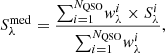 (1)
(1)
where NQSO is the number of quasars within a redshift bin and grouped into a pixel cube,  is the pixel flux density in the cutout i at a wavelength λ, and
  is the noise flux density in the same pixel. The fluxes for the different stacked maps are calculated as follows. The flux densities in the IRAC-3.6 μm, WISE-W3, MIPS-24 μm, MIPS-70 μm, PACS-100 μm, and PACS-160 μm maps are estimated using aperture photometry using radii of 2.5″, 8.5″, 22″, 30″, 5.6″, and 11.2″; respectively. The sky background is determined using inner and outer radii between 30″ and 60″. For the SPIRE maps, we fit a 2D Gaussian in addition to a constant background to the stack map and we considered the peak flux as the flux density estimate.
The density fluxes in the stacked radio maps are estimated using the relations by Condon et al. (1998). We applied a scaling factor of 12 percent to the 150 MHz LOFAR fluxes to make them consistent with the Scaife & Heald (2012) (hereafter, SH12) flux scale (Retana-Montenegro et al. 2018). The 1.4 GHz WSRT flux scale is consistent with the SH12 scale (Williams et al. 2016), while the 325 MHz VLA scale is multiplied by a factor of 0.91 to make it consistent with the SH12 scale (Calistro-Rivera et al. 2017). To investigate the consistency of the VLASS fluxes with the SH12 scale, we compute the spectral indices of VLASS sources with S/N ≥ 15 with their counterparts from the WSRT, VLA and LOFAR catalogs. We find that the mean ratio between the predicted and uncorrected VLASS fluxes is 0.91. This correction factor is used to put the VLASS fluxes to the SH12 flux scale . The 1σ errors on the median stacked fluxes are estimated using a bootstrap approach for each redshift bin. For this purpose, the sources within the redshift bin are randomly resampled (with replacement). The stacking procedure is repeated 100 times for each filter. The standard deviation of the distribution of median stacked fluxes obtained in the 100 trials is the 1σ error of the stacked flux in the corresponding filter.
Snapshot surveys with sparse UV coverage could result in a dirty beam with high sidelobes (Becker et al. 1995; Condon et al. 1998). These could be difficult to clean and could cause an underestimation of the real sources in the restored image (Condon et al. 1998). Our radio observations have good UV coverage thanks to the high integration times, thus, they are unlikely to be affected by a snapshot bias. The median stacked fluxes are not corrected for any CLEAN or snapshot bias. However, to account for any potential bias in our radio fluxes we added a 10% uncertainty in quadrature to the flux uncertainties obtained using bootstrapping. Tables 2 and 3 list the median stacked radio fluxes and noise values, respectively, for the quasar samples. The radio luminosities derived from these fluxes are shown in Fig. 5. The stacking procedure allows to detect the radio emission of RUQs that are roughly an order of magnitude less luminous than RDQs at all redshifts. The infrared fluxes are presented in Appendix B.
Radio fluxes of the median LOFAR radio-detected quasars (RDQs) and LOFAR radio-undetected quasars (RUQs) stacked according to redshift between 150 MHz and 3.0 GHz.
Noise levels (1σ) of the median radio images stacked according to redshift of LOFAR radio-detected quasars (RDQs) and LOFAR radio-undetected quasars (RUQs).
The median stacked infrared and radio images of RUQs are shown in Figs. A.1–A.3, respectively. The RUQs are detected in the majority of the filters, except in the PACS and VLASS bands where they are not detected in some redshift bins. This is somehow expected as the PACS and VLASS are relatively shallower in comparison with the other infrared and radio bands, respectively (see Sect. 2). Figures A.4–A.6 display the median infrared and radio stacked images of RDQs, respectively. In some high-z bins with a low number of RDQs stacked, the results from the median stacking are consistent with zero in the PACS and VLASS images.
4.2. Potential systematics
We verify that there is no potential bias in the median stacked fluxes by performing a null test. This test consists in stacking randomly re-positioned pairs (Zhang et al. 2013; Viero et al. 2015; Hall et al. 2019). A total of 1000 null tests are performed for each redshift bin with a number of random positions equal to the number of quasars in the bin. The stacking procedure remains identical as when the real quasar positions are used. As expected, the results of the null tests fluctuate around zero in both the infrared and radio maps. Finally, these random stacks centered around zero indicates that the contribution to our stacked fluxes of source confusion due to the blending of faint sources is negligible (Stanley et al. 2017).
Another point to consider for the radio stacking is how uniformly was the quasar sample constructed. White et al. (2007) pointed out how factors such as the SDSS quasar selection algorithm (Richards et al. 2001), or the dependency of radio and optical luminosity could affect the interpretations of the stacking analysis. Similarly, Hodge et al. (2008) found evidence for a selection bias towards bright radio sources in their stacking analysis of SDSS luminous red galaxies.
Our spectroscopic quasar sample is not uniformly constructed since it is a compilation of the observations made by way of various surveys (Cool et al. 2006; McGreer et al. 2006; Glikman et al. 2011; Kochanek et al. 2012; Pâris et al. 2018); with each survey having its own unique strategies to build its own sample. Figure 7 shows the median 150 MHz flux densities of RUQs as a function of redshift. The median 150 MHz fluxes present a trend similar to that found by White et al. (2007) in their stacking analysis of SDSS-FIRST quasars. However, we are using redshift bins broader in comparison with White et al. (2007). This yields radio fluxes that have a better agreement within the error bars except for the z ≤ 1.0 bin. Another possibility is considering only RUQs with M1450 ≤ −23.0 with △z = 1.0, where it is expected that the median fluxes are less affected by selection effects. However, it yields a result similar to what is obtained with the full RUQs sample. A possible solution could be to limit our quasar sample only to one survey with an uniform selection function, but this in return would reduce the S/N of the stacked sources, particularly for RUQs. This poorer S/N would makes our study of the RDQs and RUQs more difficult as a function of redshift and luminosity, along with its potential to investigate the origins of their radio-emission. For these reasons, we decided to use all the known spectroscopic quasars located in the WSRT-Boötes region in our stacking analysis. However, we did keep in mind that selection effects could affect (to some extent) these trends in our analysis.
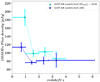 |
Fig. 7. Median-stacked 150 MHz flux densities versus redshift for all LOFAR radio-undetected quasars (RUQs) in our sample, and for RUQs with M1450 ≤ −23.0. The samples follow similar trends, indicating that selection effects could be present in both samples. |
4.3. Spectral energy distribution fitting
The observed quasar SED between mid-infrared and radio wavelengths can be fitted using three main components: AGN and SF heated thermal dust emission, and synchrotron emission. The AGN and SF heated thermal dust emission are represented as the combination of two terms (Casey 2012): a simple power-law with a low-frequency exponential cut-off that represents the AGN heated dust, and a single temperature modified blackbody (BB) that corresponds to the far-infrared emission from SF heated dust:
 (2)
(2)
where α is the power-law slope, NAGN and NBB are the normalization constants of the AGN and BB terms, λc is the fixed rest-frame cut-off wavelength, β is the emissivity index, and T is the characteristic temperature of the quasar host galaxy. The cut-off wavelength, and the emissivity are fixed to the values of λc = 45 μm and β = 2.5, respectively (Falkendal et al. 2019).
The synchrotron emission is fitted with a single power-law,
 (3)
(3)
where α is the synchrotron power-law slope, and Nsync is the normalization constant of the synchrotron term. This power-law is a simple model that can be used to determine the maximum contribution from the synchrotron emission to the radio and sub-mm frequencies.
We use Levenberg–Marquardt (LM) χ2 minimization to find the best-fitting parameters for the quasar SED model. The fitting is done using the Python implementation of the LM algorithm LmFit6. Figures 8 and 9 present the median SEDs of RUQs and RDQs, respectively in the four redshift bins, along with the best-fit SEDs and their different components. For all the SEDs, it is easy to recognize the emission associated with the hotter dust heated by the AGN, and dust heated thermally by SF, as well the synchrotron component. We also consider the possibility that the far-infrared flux densities are contaminated by synchrotron emission that is not associated with star formation. By extrapolating the fitted synchrotron power-law, we subtracted the synchrotron contribution to the far-infrared fluxes. The fitted far-infrared fluxes are fitted again to the Casey (2012) model. We verify that our results do not change significantly by using the far-infrared fluxes without subtracting the synchrotron contribution. The values of the best-fit parameters are presented in Table 4. The uncertainties are reported on the best-fit parameters correspond to 1σ errors.
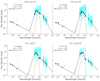 |
Fig. 8. Rest-frame spectral energy distributions (SEDs) for median LOFAR radio-undetected quasars stacked according to redshift. Black points plot the observed flux densities with downward-pointing fuchsia arrows indicating 5σ upper limits. The solid blue line shows the combined best-fit SED model, while the purple, green and orange lines show the synchrotron, black-body, and AGN best-fit components, respectively. The maroon squares indicate the predicted fluxes according to the fitted SED model. The cyan points denote the fluxes of the quasars used in the stacking. Some quasars have WSRT and VLA detections, but remain undetected in LOFAR, thus are classified as RUQS. See Sect. 3 for more details. |
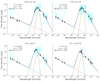 |
Fig. 9. Rest-frame spectral energy distributions (SEDs) for median LOFAR radio-detected quasars stacked according to redshift. Black points plot the observed flux densities with downward-pointing fuchsia arrows indicating 5σ upper limits. The solid blue line shows the combined best-fit SED model, while the purple, green and orange lines show the synchrotron, black-body, and AGN best-fit components, respectively. The maroon squares indicate the predicted fluxes according to the fitted SED model. The cyan points denote the fluxes of the quasars used in the stacking. |
SED model fitting results.
The total infrared luminosity of the SF (LSF) and AGN (LAGN) components are derived by integrating by separate each component of Eq. (2). The integration is done between the rest-frame wavelengths 8.0 μm and λc = 1000 μm:
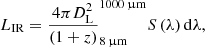 (4)
(4)
where z is the quasar redshift and DL is the luminosity distance. The total infrared luminosity, LIR, is estimated by combining the results of the SF and AGN components. Errors in the IR luminosity components are derived from the range of values obtained from SED fits which differ from the best fit by  The SF rate (SFR) of the quasars host galaxies is determined using the relation by Kennicutt (1998) assuming a Salpeter initial mass function:
![Mathematical equation: $$ \begin{aligned} \mathrm{SFR}\,\left[M_{\odot }\,\mathrm{yr} ^{-1}\right]={\displaystyle \frac{L_{\mathrm{IR} }}{5.8\times 10^{8}}}, \end{aligned} $$](/articles/aa/full_html/2022/07/aa39750-20/aa39750-20-eq32.gif) (5)
(5)
where LIR is in units of solar luminosities, L⊙. The infrared luminosities and SFR estimates are listed in Table 4.
We also fit the radio-infrared photometry of the individual quasars to Eqs. (2) and (4). For quasars that are undetected in the radio and infrared bands, we determined the upper limits using forced photometry measurements at their optical positions in the infrared and radio maps. We calculate the upper limits in the radio maps considering apertures that are slightly smaller to the corresponding beam sizes (see Sect. 2) to prevent these measurements to be affected by imaging artifacts. These fluxes are used as upper 5σ limits in the SED fitting.
5. Results
5.1. Far-infrared radio correlation
The far-infrared radio correlation (FIRC) is an indicator that is regularly used to investigate the levels of SF and AGN activity in galaxies (Helou et al. 1985; Condon 1992; Yun et al. 2001; Bell 2003). Particularly, the FIRC of normal star-forming galaxies, namely, those without significant AGN activity, is a tight relation with a scatter of less 0.3 dex over five orders of magnitudes in luminosity (Yun et al. 2001). This is thought to be the result of the infrared and radio emission being related to the rate of massive star formation (Condon 1992).
The FIRC is parametrized using the dimensionless parameter, qFIR, that is defined as (Helou et al. 1985; Yun et al. 2001):
 (6)
(6)
where LIR is the rest-frame infrared luminosity from 8.0 μm to 1000 μm, and LRadio is the radio luminosity at a certain frequency.
In Fig. 10, we plot the median infrared and radio luminosities along with upper limits on the luminosities for the individual quasars that are undetected by LOFAR, WSRT, and SPIRE at 250 μm. Also we compare our results with the FIRC results obtained by Calistro-Rivera et al. (2017) for star-forming galaxies at 150 MHz and 1.4 GHz in the NDWFS-Boötes field. We define a quasar to be SF-dominated if the quasar is within a factor of ±2 of the expected value predicted by the FIRC. In both panels of Fig. 10, the most striking result is that median RUQs that are stacked according to redshift closely follow the FIRC as it is expected for normal star-forming galaxies. We did not observe any redshift trend for median quasars. In the right panel, the median RDQ in the lowest redshift bin is located closer to the FIRC prediction with their radio-emission likely to have a significant contribution of SF, while the remaining three redshift bins are located far to the right side of the FIRC. The significant excess exhibit in their radio luminosities emission is greater than the levels expected from SF activity alone and most likely can be associated with AGN activity. Therefore, the radio fluxes of the mean RDQs in the three highest redshift bins could be considered as AGN-dominated. The upper limits on the infrared and radio luminosities of the individual RUQs are insufficient to determine individually how closely each one of these objects follow the FIRC. In Fig. 10 (right panel), there are a few quasars that that are undetected by LOFAR, but are detected by WSRT at 1.4 GHz (purple and blue circles). We classify these quasars as RUQs due to being undetected by LOFAR at 150 MHz (see Sect. 3), but they show radio-excess (i.e., radio emission associated with radio jets). Finally, in both panels the individual RDQs also present radio-excess at 1.4 GHz which suggests that their radio fluxes are AGN-dominated. This is consistent with the results obtained in Sect. 6.2, where it is found that the fraction of RDQs that is AGN-dominated at 150 MHz (1.4 GHZ) is 67% (85%).
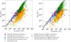 |
Fig. 10. Comparison between infrared luminosity, LIR, and radio luminosity at 150 MHz and 1400 MHz. Left: LIR versus the radio luminosity at 150 MHz. LIR and L150 MHz are in units of solar luminosity. Measurements for median LOFAR radio-undetected quasars (RUQs, fuchsia and cyan squares), median LOFAR radio-detected quasars (RDQs, red and turquoise stars), RDQs detected by SPIRE at 250 μm (maroon stars), RUQs detected by SPIRE at 250 μm (yellow circles), and RUQs undetected by SPIRE at 250 μm (green circles) are shown. Upper limits are indicated by arrows in either LIR or L150 MHz. For median quasars, the increasing symbol size indicates an the increment in redshift or M1450 absolute luminosity. The dashed line is the far-infrared radio correlation (FIRC) at L150 MHz derived by Calistro-Rivera et al. (2017). The gray shaded region indicates the spread of the FIRC scaled by a factor of ±2. The text indicates the median redshift of the first and last redshift bins of the stacking according to redshift. Right: Same as the right panel, but for the radio luminosity at 1400 MHz, L1400 MHz. Measurements for RUQs detected by WSRT, but undetected by SPIRE at 250 μm (purple circles); and RUQs detected by both SPIRE and WSRT at 250 μm and 1400 MHz (blue circles), respectively are also displayed. |
We also examined the behavior of the infrared and radio luminosities as a function of the 1450 Å absolute magnitude. For this purpose, we stacked our sample following the steps explained in Sects. 4.1 and 4.3, namely, as a function of 1450 Å absolute magnitude. We use bins of size △M1450 = −1.0 for RUQs, and △M1450 = −2.0 for RDQs to account for the smaller size of the RDQs sample. In all flux-limited samples, the luminosities are correlated with redshift, which is driven by the apparent lack of bright low-z sources, and faint sources at higher redshifts due to the detection limits. Thus, we keep in mind that there is a possibility that the faintest bins are affected by some incompleteness. Figure 10 shows that median RDQs ad RUQs stacked according to their M1450 luminosity follow similar trends to those found in the stacking according to their redshift. In the same plot, we find that the main difference is that the radio-emission of median RDQs in the faintest M1450 bin is clearly AGN-dominated. In contrast with the results of the lowest z-bin where the radio-emission is probably SF-dominated. We did not find any M1450 trend for median quasars.
5.2. Star formation rates and stellar masses
In this section, we compare the SFRs derived using the infrared luminosity LIR (see Sect. 4.3) and the radio luminosities at 150 MHz and 1.4 GHz to investigate the origins of the radio-emission in RUQs. Both SFR estimates are derived independently. The SFR estimate derived from radio observations, SFRRadio, is obtained assuming that the synchrotron emission produced in the host galaxies of RUQs is associated with supernova remnants with short cooling times. Thus, the radio emission can be considered as a measure of the instantaneous SFR in the host galaxy (Condon 1992). From the 1.4 GHz radio luminosity, L1.4 GHz, this is carried out using the following relation (Yun et al. 2001):
![Mathematical equation: $$ \begin{aligned} \mathrm{SFR} _{\mathrm{Radio} }\,\left[M_{\odot }\,\mathrm{yr} ^{-1}\right]=5.9\times 10^{-22}\times {\displaystyle L_{1.4\,\mathrm{GHz}}}. \end{aligned} $$](/articles/aa/full_html/2022/07/aa39750-20/aa39750-20-eq34.gif) (7)
(7)
The SFR from the 150 MHz radio luminosity, L150 MHz, is calculated using the relations presented by Calistro-Rivera et al. (2017). These relations were derived using early LOFAR radio-continuum observation of the NDWFS-Boötes field (Williams et al. 2016) for a sample of spectroscopic galaxies between 0 ≤ z ≤ 3.5.
In Fig. 11, we compare the SFRs derived from the infrared and radio luminosities. We also plot the FIRC correlation for star-forming galaxies (from Calistro-Rivera et al. 2017) to establish whether or not SF could account for the radio-emission in RUQs. In agreement with our results of the Sect. 5.1, we find that the data points of the median RUQs stacked according to their redshift lie along the FIRC at 150 MHz. However, the data point at z = 0.7 (see text in right panel. Fig. 10) shows a slightly larger scatter than the rest of the other data points at 1.4 GHz. However, these results suggest that the SFRs of the median RUQs agree with the predictions of the FIRC. Their radio-emission could be explained by star-forming processes assuming that the FIRC is a valid indicator to determine the origins of the radio-emission in RUQs (see discussion in Sect. 6.2). The situation for the RUQs with upper limits on 250 μm and radio bands is more difficult to assess on a per-source basis. The upper limits only indicate that these sources could be located close to the FIRC but their exact location in the SFRRadio − SFRIR plane is uncertain without deeper observations. The majority of RUQs detected by WSRT (purple circles), but not by LOFAR show values that exceed the predictions of the FIRC, thus, their radio-emission is above that expected from star formation alone suggesting that it is AGN-dominated. At 150 MHz, the median RUQs stacked using M1450 present a trend that is similar to that found when the stacking is done according to redshift with values following the FIRC predictions. At 1.4 GHz, the M1450 -stacked RUQs have SFR1.4GHz values larger than the FIRC predictions. However, these values are still consistent with being dominated by SF. In summary, the trends found for the SFRs are similar to those found in Sect. 5.1 with the comparison between the infrared and radio luminosities.
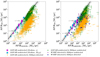 |
Fig. 11. Comparison between star-formation rates (SFRs) derived using infrared and radio data. Left: SFR derived from the infrared luminosity, SFRIR, versus the SFR derived from the radio luminosity at 150 MHz. SFRIR and SFR150 MHz are in units of solar mass per year. The measurements for median LOFAR radio-undetected quasars (RUQs) (fuchsia and cyan squares), RUQs detected by SPIRE at 250 μm (yellow circles), and RUQs undetected by SPIRE at 250 μm (green circles) are showed. Upper limits are indicated by arrows in either SFRIR or SFR150 MHz. For median quasars, the increasing symbol size indicates an increment in the redshift or M1450 absolute luminosity. The dashed line is the far-infrared radio correlation (FIRC) at L150 MHz derived by Calistro-Rivera et al. (2017). The gray shaded region indicates the spread of the FIRC scaled by a factor of ±2. The text indicates the median redshift of the first and last redshift bins of the stacking according to redshift. Right: Same as the right panel, but for the SFR at 1400 MHz, SFR1400 MHz. The measurements for RUQs detected by WSRT, but undetected by SPIRE at 250 μm (purple circles); and RUQs detected by both SPIRE and WSRT at 250 μm and 1400 MHz (blue circles), respectively are also displayed. |
The distribution of the SFRs in our quasar sample derived using the infrared luminosity LIR is shown in Fig. 12. Only quasars detected by SPIRE at 250 μm at ≥2σ significance are plotted in order to have robust estimations of the SFRIR. The mean SFRIR of the RUQs with S250 μm detections is 149 M⊙ yr−1, while the corresponding SFRIR of RDQs is 196 M⊙ yr−1. These values are consistent with the median SFRsIR of the median quasars, which are 125 M⊙ yr−1 and 267 M⊙ yr−1 for RUQs and RDQs, respectively. It is clear that with SFRs of only a few hundred M⊙ yr−1, the SF processes occurring in the quasars in our sample is less vigorous in comparison with other far-infrared sources with very powerful ongoing starbursts such as sub-millimeter galaxies (Wardlow et al. 2011; Fu et al. 2013; Barger et al. 2014), and luminous optical quasars (Pitchford et al. 2016; Trakhtenbrot et al. 2017; Duras et al. 2017). These sources usually present SFRs at the level of thousands of M⊙ yr−1 at redshifts z > 2. These powerful starbursts are associated with the most massive and rarest galaxies at any redshift (Baldry et al. 2012; Ilbert et al. 2013) and, therefore, they have low spatial densities. Due to these low numbers their potential contribution to our median SFR measurements is negligible.
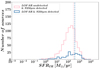 |
Fig. 12. Infrared star formation rate (SFR) distribution for the RDQs and RUQs derived from the infrared luminosity LIR with ≥2σ SPIRE-250 μm detections. The mean SFR of the samples are indicated by the dashed lines. The mean SFRs of our quasar samples are consistent with those of the main sequence star-forming galaxies. |
In Fig. 13, we display the SFRsIR derived from the infrared luminosities, as a function of redshift for RUQs and RDQs. For the sake of clarity, only objects with SPIRE 250 μm detections at ≥2σ are plotted. The larger symbols represent the measurements obtained from the stacking analysis. We see an increase in the median SFRIR of quasars with cosmic look-back time. At z ∼ 0.6, we find the median SFRIR of RDQs (RUDs) to be 
 , whereas at z ∼ 1.35 the increment is approximately seven (four) times greater, and in our high-z bins at z ∼ 2.16 and z ∼ 3.2 the SFRIR is thirty four (twenty five) times greater. These ranges of median SFRIR are wide, however, the trend of median SFRIR increasing with redshift in quasars is clear and consistent with previous studies (Seymour et al. 2011; Kalfountzou et al. 2014; Stanley et al. 2017). Finally, RDQs present higher SFRIR values than RUQs at all redshifts, except at the last z-bin where the SFRIR values between the two quasar samples are consistent taking into account the error bars.
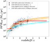 |
Fig. 13. Infrared star formation rate (SFRIR) of LOFAR radio-detected quasars (RDQs) and LOFAR radio-undetected quasars (RUQs) versus redshift. The filled stars and squares and associated vertical error bars show the median value in each bin. The horizontal error bars indicate the extend of the redshift bins used. The marron stars and cyan squares show the results for the RDQs and RUQs, respectively, with ≥ 2σ SPIRE-250 μm detections. The solid lines represent the predicted SFRs as a function of redshift derived for the median quasars using the star-formation main sequence (SFMS) relation by Schreiber et al. (2015). The cyan and orange shaded regions indicate the uncertainty intervals of the fitting provided by Schreiber et al. (2015). The vertical errror bars indicate the errors of the SFRIR estimates obtained using the SED fitting, while the horizontal errors indicate the size of the redshift intervals considered. There is a good agreement between the measured median SFRIR for RDQs and RUQs, and the SFMS predictions considering the width of the redshift bins employed and the intrinsic scatter of the SFMS relation. |
Studies of star-forming galaxies at a wide range of cosmic epochs have revealed a strong correlation called the SF main sequence (SFMS, hereafter) at fixed redshift between SFR and stellar mass (M*). This relationship has been shown to hold over four to five orders of magnitude in mass (Santini et al. 2009, 2017) and from z = 0 to z = 6 (Noeske et al. 2007; Daddi et al. 2007; Steinhardt et al. 2014; Speagle et al. 2014; Schreiber et al. 2015), with only a scatter of 0.25−0.35 dex at any redshift (Daddi et al. 2007; Whitaker et al. 2012). Using the SFMS formula derived by Schreiber et al. (2015), we find that the median stellar masses of the median RUQs and RDQs are M* ∼ 5 × 10¹⁰ M⊙ and M* ∼ 3 × 10¹¹ M⊙, respectively. The solid lines represent the SFRs as a function of redshift derived for the median quasars using the Schreiber et al. (2015) relation. There is a good agreement between the measured median SFRIR for RDQs and RUQs, and the SFMS predictions considering the width of the redshift bins employed and the intrinsic scatter of the SFMS correlation. The differences in the scatter between RDQs and RUQs could be explained considering that the former includes almost entirely quasars that might be located in massive galaxies due to the radio-selection being associated with massive systems (Retana-Montenegro & Röttgering 2017; Magliocchetti et al. 2020). The latter includes quasar host galaxies with a wide range of stellar masses. Thus, for galaxies hosting RUQs a larger scatter with respect SFMS could be expected due to the wide range of stellar masses included in the sample. We conclude the SFRsIR and stellar mass measurements of galaxies hosting RUQs and RDQs are broadly consistent with those of massive star-forming galaxies following the main sequence. Moreover, these estimates are in good agreement with previous works of main sequence galaxies at 0.2 < z < 2.5 (Rosario et al. 2013; Stanley et al. 2017; Schulze et al. 2019). Additionally, the stellar masses of the quasar host galaxies in our sample aligns well with those estimated for z < 0.8 quasars obtained using image decomposition in CFHT (Yue et al. 2018) and SDDS S82 deep imaging (Matsuoka et al. 2014; Bettoni et al. 2015). These authors found stellar masses larger than M* > 1010 M⊙ for the quasar host galaxies, but no distinction was made between radio-detected and radio-undetected objects.
5.3. Median star formation rate as a function of optical and radio luminosities
In this section, we examine the behaviour of the SFR as a function of the 1450 Å absolute magnitude and 150 MHz radio luminosities. For this purpose, we stacked our sample following the steps explained in Sects. 4.1 and 5.1 as a function of 1450 Å absolute magnitude and 150 MHz radio luminosity. We used bins of size ▵log L150 MHz = 1.0 for the radio luminosity, and we use the same bin sizes for M1450 that was employed in the previous section.
Figure 14 shows the distributions of 1450 Å absolute magnitudes, 150 MHz radio luminosities, and SFRsIR. Both panels shows a correlation between median optical and 150 MHz radio luminosites and SFR for quasars which extends over more than two orders of magnitude in SFRIR. The first thing that comes to mind are the similarities and differences between the behavior of the median RDQs and RUQs. The first similarity is that both median quasar samples present a positive trend of SFRIR as function of the 1450 Å absolute magnitude in which SFRIR increases with M1450. The main difference is that for M1450 ≥ −24.0 median RDQs (red stars) have higher SFRsIR in comparison with their radio-undetected counterparts (gray squares). For M1450 ≤ −24.5 median RDQ and RUQs present similar SFRIR values within their corresponding uncertainties. This agrees with previous results found by Kalfountzou et al. (2014) for RLQs and RQQs. These authors found that RLQs present higher SFRs than RQQs at low and medium optical luminosities but have comparable SFRs at high optical luminosities.
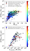 |
Fig. 14. Infrared star-formation rates (SFRsIR) versus absolute magnitude at 1450 Å, M1450, (top panel) and 150 MHz radio luminosity (bottom panel) for LOFAR radio-detected quasars (RDQs) and radio-undetected quasars (RUQs). Only RDQs (stars) and RUQs (squares) with ≥ 2σ SPIRE-250 μm detections are shown (see Sect. 2.3). For median quasars, the increasing symbol size indicates an increment in the redshift, M1450 absolute luminosity, or 150 MHz radio luminosity. The errors on the horizontal axis indicate the extend of the luminosity bins used. Vertical error bars are the 1σ uncertainties for the SFRsIR obtained from the SED fitting. The positive correlation between optical and radio luminosities suggest that there is a link between their SFR and AGN activity in median RDQs and RUQs, with indications of star formation being suppressed in the host galaxies of the most luminous radio quasars. |
Assuming that the far-infrared is a good proxy of SF, we conclude that these trends discussed before suggest that there is a link between their SFR and AGN activity in median RDQs and RUQs. Previous studies found a correlation between the far-infrared and accretion luminosities, supporting the idea that SF and AGN activity share the same reservoir of cold gas in the host galaxy (e.g., Serjeant & Hatziminaoglou 2009; Lutz et al. 2010; Bonfield et al. 2011). It is possible that the different efficiencies in which gas fuels SF and AGN processes or the heating of gas via feedback processes may explain the observed behaviors in the SFRIR − M1450 correlation. The existence of gas reservoirs similar to those of non-active galaxies has been confirmed in low-z (Shangguan et al. 2020) and high-z (Riechers et al. 2011; Fogasy et al. 2020; Badole et al. 2020) quasars. However, CO observations are required to determine better constraints for quasar sample.
In the bottom panel of Fig. 14, we show the distribution of median SFRsIR for RDQs as a function of 150 MHz radio luminosity. We also plot for reference the results for median RUQs (median stacked by redshift bins) and SPIRE-250 μm detections. We find again a rise in the SFRIR with increasing 150 MHz radio luminosity. Median RUQs are shifted to the left as expected due to being less luminous in the radio in comparison with the median RDQs. We see that median RDQs preset a flattening, or possible decline in SFRIR in the highest L150MHz bin. This decline roughly coincides with the spread of the individual detections. This contrasts with the top panel of Fig. 14 that shows no downturn in SFRIR at the highest M1450 values. This perhaps could indicate that SF is suppressed in host galaxies of luminous radio quasars due to the impact of radio-jets. Additionally, this is consistent with the trend found in the left panel of Fig. 10: the radio-emission of the most luminous RDQs exceeds the FIRC predictions and it is likely AGN-dominated (discussed in more detail in Sect. 6.3).
5.4. Redshift evolution of the radio spectral indices
We calculated the spectral index between adjacent frequency pairs at 150 MHz, 325 MHz, 1.4 GHz and 3.0 GHz. For quasars that are undetected, we derived an upper limit for the spectral index when the quasar is only detected in one (two) frequency (ies) in the pair. The spectral indices are calculated using the formula:
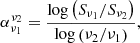 (8)
(8)
where  is the spectral index between the corresponding frequencies, Sνi denotes the flux density at frequency vi. In the cases of non-detections, we use forced photometry in the corresponding frequency (ies) as described in Sect. 4.3. The redshift evolution the spectral indices are presented in Figs. 15 and 16 for RDQs and RUQs, respectively. For RDQs, it can be seen that the results for median RDQs within errors are consisted with no evolution a function of redshift for the three spectral indices. The robustness of this result is verified by fitting a straight line to the data points. It is found that the slope of the straight line is close to zero, which rules out a redshift evolution for the spectral indices. This agrees with previous studies that found no evidence for the redshift evolution of the radio spectral indexes (Magnelli et al. 2015; Calistro-Rivera et al. 2017). The spectral indices of the RDQs detected show scatter around the values obtained from the stacking analysis, while the RDQs with upper limits are still consistent with these values although with a larger dispersion.
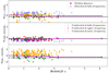 |
Fig. 15. Evolution of spectral indexes α3.0−1.4 (top), α1400−325 (middle), and α325−150 (bottom) as a function of redshift for LOFAR radio-detected quasars (RDQs). The purple circles represent the median RDQs; green circles are the RDQs detected at both frequencies; yellow or red circles indicated RDQs that are undetected in the upper or lower frequency, respectively; and blue circles are RDQs undetected at both frequencies. The horizontal dashed line indicates the canonical value of α = −0.7. |
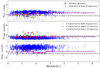 |
Fig. 16. Evolution of spectral indexes α3.0−1.4 (top), α1400−325 (middle), and α325−150 (bottom) as a function of redshift for LOFAR radio-undetected quasars (RUQs). The purple circles represent the median RUQs; green circles are the RUQs detected at both frequencies; yellow or red circles indicated RUQs that are undetected in the upper or lower frequency, respectively; and blue circles are RUQs undetected at both frequencies. The horizontal dashed line indicates the canonical value of α = −0.7. |
We also note that for median RDQs the mean for the spectral index between 325 MHz and 1.4 GHz,  , is steeper than the canonical value of α = −0.7 used in previous radio continuum studies with a value of
  . For comparison, our result is in good agreement with the published mean value by Sirothia et al. (2009) of
  , but it is steeper than the mean value reported of
  by Mauch et al. (2013) for all radio sources in their corresponding catalogs. For median RUQs, the mean spectral index is steeper with a value of
  . The spectral index between 1400 MHz and 3000 MHz,
  , for median RDQs has a value of
  , while for median RUQs the shallower flux density limit of the 3.0 GHz VLASS mosaic makes only possible to obtain an estimate with > 3σ significance in one redshift bin. For the remaining three redshift bins only upper limits are estimated. The mean spectral index of median RUQs is
  , calculated using the Kaplan-Meier estimator (e.g., Feigelson & Nelson 1985) to account for the upper limits. Our values are flatter in comparison to the mean value of
  found by Smolčić et al. (2017). We find that that the mean spectral index between 325 MHz and 150 MHz,
  , has a value of
  (−0.11 ± 0.03) for median RDQs (RUQs). In contrast, these values are flatter than those reported by Calistro-Rivera et al. (2017) of
  and
and  for AGN and star-forming galaxies, respectively. However, our results are consistent with the spectral flattening of radio sources towards low-frequencies previously observed in LOFAR (van Weeren et al. 2014; Mahony et al. 2016) and GMRT (Intema et al. 2011; Williams et al. 2013) observations.
6. Discussion
The stacking technique is an important tool in understanding the nature of radio emission in quasars, as basically all quasars emit in the radio when observed down to deep limits. In this work, we find evidence for concurrent AGN and star-forming activity in the host galaxies of median-stacked quasars with a positive correlation between SFRIR and optical and radio luminosities. These pieces of evidence suggest that the radio-emission in quasars is the result of a complex interplay between SF and SMBH accretion processes with each process having significant contributions to the quasar energy output. In this section, we discuss and interpret our findings.
6.1. No bimodality for the radio-loudness parameter
Here, we investigate the radio-loudness parameter using the results of our analysis stacking, and discuss the origins of the radio-emission in quasars with the lowest radio-loudness values. We define the radio-loudness parameter (R hereafter) for our quasar samples using the ratio of radio to infrared AGN luminosity:
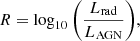 (9)
(9)
where Lrad is the radio luminosity at 150 MHz or 1.4 GHz, and LAGN is the infrared AGN luminosity estimated in Sect. 4.3. We decided to use the infrared AGN luminosity instead of an optically derived luminosity. This is done because the mid-infrared continuum of the majority of quasars arises from dust heated by the central AGN (Richards et al. 2006; Gallagher et al. 2007). This makes the mid-infrared luminosity robust against extinction effects.
In Sect. 5.1, we demonstrate that the SF could dominate the radio-emission of RUQs and a significant fraction of RDQs. As explained in Sects. 5.1 and 5.2, we define a quasar to be SF-dominated if the quasar is within a factor of ±2 of the expected value predicted by the FIRC. Figure 17 shows the ratio of LSF/Lrad as a function of R for our quasar samples. The FIRC is denoted by a solid line in both panels, and the shaded gray horizontal regions indicate the FIRC scaled by a factor of ±2. The dashed vertical lines indicates the thresholds of R = −4.5 (150 MHz) and R = −4.2 (1.4 GHz) utilize to classify quasars into radio-loud/radio-quiet (e.g., Klindt et al. 2019; Rosario et al. 2020). We see in both panels of Fig. 17 that median RUQs (stacked according to their redshift and M1450) and a significant fraction of RDQs have R values below the thresholds at 150 MHz and 1.4 GHz. These quasars would be classified as radio-quiet in previous works. Moreover, many of these quasars fall within the region delimited by ±2 FIRC factors suggesting that their radio emission dominated by SF, which is in agreement with the results obtained in Sect. 5.1. On the other hand, the radio fluxes of median RDQs (stacked according to their redshift and M1450) are AGN-dominated according to their location outside the predictions of the FIRC. However, some of them have R values below the classification thresholds. It is clear that there is a trend for RDQs with high R values (thus high radio-luminosities) to have their radio-emission dominated by SMBH accretion. This should not come as a surprise, based on their predominant FR-II-like (Fanaroff & Riley 1974) radio-morphologies. Representative examples of their radio-morphologies can be found in Retana-Montenegro & Röttgering (2020), Appendix A. On the other side, for low R values ≤ − 4.5, around 50% of the RDQs have faint and compact radio morphologies suggesting that AGN processes are not longer dominating the radio-emission as they do at higher R values. For these RDQs, the relative contribution to the radio emission due to SF increases as the AGN component becomes weaker towards lower R values. Finally, we also notice that WSRT RUQs (blue circles, right panel) show a similar trend to that of the LOFAR RDQs (maroon stars, left panel). For the majority of individual RUQs it is difficult to make an assessment as these are non-detections in the LOFAR, WSRT, and S250 μm bands and only upper limits can be estimated on their R and LSF/Lrad values. However, most likely these quasars follow a similar trend and occupy a comparable region to that of the median RUQs (stacked according to redshift and M1450).
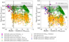 |
Fig. 17. Infrared star formation luminosity, LSF, versus radio-loudness, R, for the quasar samples. The measurements for median LOFAR radio-undetected quasars (RUQs, fuchsia squares), median LOFAR radio-undetected quasars (RDQs, red stars), RDQs (maroon stars) and RUQs detected by SPIRE at 250 μm (orange circles), and RUQs undetected by SPIRE and WSRT at 250 μm and 1.4 GHz (green circles), respectively. The measurements for RUQs detected by WSRT, but undetected by SPIRE at 250 μm (purple circles, right); and RUQs detected by both SPIRE and WSRT at 250 μm and 1.4 GHz (blue circles, right), respectively are also displayed. Upper limits in either LSF or L150 MHz are indicated by arrows. The solid line is the far-infrared radio correlation (FIRC) at 150 MHz and 1.4 GHz. The gray shaded region indicates the spread of the FIRC scaled by a factor of ±2. The dashed vertical lines (R = −4.5 at 150 MHz and R = −4.2 at 1.4 GHz) denote the threshold between radio-loud and radio-quiet quasars (see Sect. 6 for more details). The radio-emission of bright RDQs with R ≳ −4.5 is consistent with being dominated by SMBH accretion, while for lower radio luminosity quasars with R < −4.5 the relative contribution of SF to their radio fluxes becomes more important. |
Another important conclusion that can be inferred from Fig. 17 is the high fraction of RDQs with values of R ≤ −4.5 (R ≤ −4.2) is 55% (53%) at 150 MHz (1.4 GHz), respectively. Specifically, the fraction of SF-dominated RDQs at 150 MHz (1.4 GHz) with R ≲ −4.5 (R ≲ −4.2) is 28% (13%). The higher sensitivity of LOFAR for objects with typical synchrotron spectra makes possible to detect the radio emission of a significant number of these quasars. Figure 18 shows the distribution of the R parameter for the RDQs samples in our study. It can be seen that the distributions of all RDQs and SF-dominated RDQs with R ≤ −4.5 present no obvious bimodality, while the distribution of AGN-dominated RDQs with R > −4.5 exhibits two peaks. We fit these distributions to a single Gaussian and a two-component Gaussian mixture using Markov chain Monte Carlo. The odd ratio for the models is O12 ≳ 1.0, which suggests that neither model is favored by the data. This suggests that the distribution of the R parameter is not bimodal, and there is not a dichotomy as previously reported in the literature (e.g., Kellermann et al. 1989; Miller et al. 1990; White et al. 2007). Our result agrees with previous works where the R parameter exhibits a continuous distribution rather than a clear bimodality (e.g., Lacy et al. 2001; Gürkan et al. 2019; Fawcett et al. 2020).
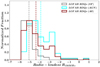 |
Fig. 18. Distributions of the radio-loudness parameter, R, derived using the 150 MHz radio luminosity for different LOFAR radio-detected quasar (RDQs) samples. The means of each distribution is indicated by the corresponding dashed line. |
6.2. Origins of the radio-emission in radio-undetected quasars: Dominant mechanism or complex interplay
The dominant mechanism responsible for the bulk of the radio-emission in RQQs is a matter of ongoing debate. Many recent studies had pointed towards synchrotron emission from SF processes as the mechanism source of radio emission in RQQs (see Padovani 2016 for a review). However, the presence of weak small-scale radio jets in RQQs points towards a non-thermal origin for their radio emission (Leipski et al. 2006; Herrera Ruiz et al. 2016). The comparison between the VLBI and lower-resolution VLA images indicate that around ∼25−50% of the radio emission in these quasars could originate from star-forming processes (Herrera Ruiz et al. 2016). Similar conclusions have been reached by other VLBI studies of RQQs and radio-quiet AGN (Ulvestad et al. 2005; Maini et al. 2016).
Various studies of RQQs have provided different hints on the origins of their radio-emission. For instance, White et al. (2017) analyzed a sample of SDSS 70 RQQs at z ∼ 1 and found that their RQQs showed an excess of radio emission compared to that expected from the FIRC, which cannot be explained by SF alone. These authors concluded that AGN processes could account for ∼80% of the total radio luminosity in over 90% of the RQQs included in their sample. A similar conclusion was reached by White et al. (2015) using the radio-stacking technique with 1.4 GHz VLA observations. Kimball et al. (2011) constructed the 6.0 GHz radio-luminosity function from a sample of SDSS quasars at 0.2 ≤ z ≤ 0.3. These authors concluded that quasars with L6.0 GHz ≤ 1022.5 WHz−1 are mainly driven by SF, while at L6.0 GHz > 1022.5 WHz−1 the luminosity is related to SMBH accretion. Moreover, the advent of deep radio surveys offers the possibility of performing studies that are complementary to the aforementioned works. For instance, Padovani et al. (2015) and Bonzini et al. (2015) found that significant numbers of radio-quiet AGN are powered mainly by star-forming processes using deep 1.4 GHz VLA observations of the E-CDFS region.
The analysis presented in Sects. 5 and 6.1 indicates that median RUQs does not show radio excess according to the FIRC. This suggests that radio emission in the RUQs included in our sample is to a certain amount powered by star formation in their host galaxies (e.g., Padovani et al. 2015; Alberts et al. 2020; Algera et al. 2020). On the other hand, the radio fluxes of the majority of RDQs in our sample show a radio excess which could be considered as evidence that supports radio activity related to radio-mode feedback (Hardcastle et al. 2007; Heckman & Best 2014). However, the remaining 33% of RDQs in our sample do not show an radio excess, possibly related to the weakening of the AGN component contributing to their radio emission towards lower R values.
We establish the level of contribution of AGN accretion and SF to the radio-emission of median quasars by calculating the radio luminosity associated with AGN accretion L150 MHz, acc:
 (10)
(10)
where L150MHz is the total radio luminosity, and L150MHz, SF is the radio luminosity connected to SF estimated using the FIRC. For the median RDQs stacked according to redshift, we find that the accretion-related radio luminosity accounts for 45.3−81.1% the total radio luminosity at 150 MHz. These percentages for median RDQs stacked according to M1450 and 150 MHz radio luminosity are 49.5−72.4% and 56.2−97.2%, respectively. We repeat the same calculation for median RUQs, but these quasars are SF-dominated and except for one have a negligible contribution from AGN accretion to their radio-fluxes, resulting in unphysical L150MHz, acc values according to the definition in Eq. (10). Instead we used the 1400 MHz radio luminosity to calculate the percentage of radio luminosity due to AGN accretion. The resulting estimate for the percentage of accretion-related 1400 MHz radio luminosity in median RUQs stacked according to redshift (M1450) is 5.4−41.6% (3.8−40.2%). Interestingly, our findings for RDQs are comparable to those of Herrera Ruiz et al. (2016) and White et al. (2017), who showed that AGN accretion can account ∼50−83% of the total radio-emission in their RQQs sample. Finally, we obtained similar percentages at 1400 MHz for RDQs to those found at 150 MHz.
The percentages found here are within what is expected from our results. Median RUQs exhibit lower percentages of accretion-related radio–emission in comparison with median RDQs, with some RUQs almost being dominated by SF according to the FIRC derived by Calistro-Rivera et al. (2017) at 150 MHz. Median RDQs present higher percentages of accretion-related radio–emission but still the contribution of SF to their total radio luminosity is non-negligible. From our results, it is clear that the radio luminosity in quasars is the result of a complex interplay between SF and SMBH accretion with each process having a non-negligible contribution.
Finally, an important point to be considered is the use of the FIRC to determine the main radio-emission mechanism in quasar samples. While, it has been shown that the FIRC holds for star-forming galaxies fainter than ≲150 μJy using both stacking (Garn & Alexander 2009) and individual detections (Mauch et al. 2020), this correlation could have an intrinsic bias as the influence of AGN on the SFRs could affect control samples of non-active star-forming galaxies (Scholtz et al. 2018). For instance, recent VLBI observations revealed unambiguous evidence for jet activity in the lensed RQQ HS 0810+2554 (Hartley et al. 2019). With a flux density of only 880 nJy at 1.65 GHz, this is the faintest radio quasar observed until now. Moreover, it was found that the host galaxy of this lensed quasar follows the FIRC as it does not display the radio-excess typically associated with AGN activity (Stanley et al. 2017). These findings suggest that radio jet production is able to coexist alongside star-forming activity in the faintest radio quasars despite their host galaxies follows the FIRC. This makes clear that the FIRC must be used with caution to determine the main radio emission mechanism in RUQs. The question of what is the contribution of radio-jets to the energy output of RUQs could be only answered satisfactorily with future high-resolution radio observations.
6.3. Positive and negative AGN feedback
We find in Sects. 5.2 and 5.3 (see Figs. 13 and 14) that the median host galaxies of RDQs are associated with higher SFRsIR than median RUQs. Excluding the highest M1450 and z bins where less sources are found, which produces larger error bars for the SFRIR estimates, the SFRsIR of median RDQs are at least larger by a factor of 2 than those of median RUQs. These results demonstrate that vigorous SF activity is coeval with the growth of the SMBHs residing in the nuclei of the RLQs host galaxies. This agrees with previous works that found evidence for high SFRs in radio AGN (e.g., Seymour et al. 2011; Podigachoski et al. 2015; Magliocchetti et al. 2014, 2016, 2020). Moreover, bright RDQs have been associated with higher SFRs in comparison to their radio-quiet counterparts (e.g., Kalfountzou et al. 2014, 2017). The enhancement in the star formation in radio AGN could be explained considering the formation of bow shocks caused by radio jets that compress the interstellar medium in the host galaxy. This compression results in higher gas clumping leading to an increased SF efficiency (Klamer et al. 2004; van Breugel et al. 2004; Gaibler et al. 2012; Ishibashi & Fabian 2012). Observational studies support the existence of jet-induced star formation (positive feedback) in the local universe (Minkowski’s object; Croft et al. 2006; Centaurus A; Mould et al. 2000; Salomé et al. 2017), at intermediate redshift (PKS2250-41; Inskip et al. 2008) and high redshift (4C 41.17; Dey et al. 1997). While our results suggests that jet-induced SF could be taking place in our RDQs sample, it is important to remark that the conditions under which radio jets would enhance the SF are not completely understood yet.
Another critical aspect to understand AGN feedback in RUQs and RDQs are the differences between their host galaxies. Particularly, radio AGN such as radio-galaxies and bright RDQs are known to populate overdense regions (Venemans et al. 2007; Falder et al. 2010; Retana-Montenegro & Röttgering 2017) and are usually associated with massive galaxies (Falkendal et al. 2019; Best et al. 2005). In Sect. 5.2, we show how the SFRsIR of the median-stacked quasars in our sample follow the SFMS predictions with median stellar masses of M* ∼ 3 × 10¹¹ M⊙ and M* ∼ 5 × 10¹⁰ M⊙ for RDQs and RUQs, respectively. The former have the higher stellar masses comparable to those of the most massive galaxies (Caputi et al. 2011; Labbé et al. 2005), while the latter have lower stellar masses consistent with the mass scale associated with quasar hosts (Rosario et al. 2013; Matsuoka et al. 2014). Additionally, this difference is in line with what has been found by previous studies of the host galaxies of radio sources (e.g., Smolčić 2009; Best & Heckman 2012; Delvecchio et al. 2017). Finally, as can be seen in Fig. 13, the star-forming properties of the median RDQs hosts are similar to those of the general population of massive normal (i.e., non-quasar) galaxies at comparable redshifts. This indicates that there is no quenching of star formation in the median RDQs hosts with median stacking carried out according to redshift and M1450 in all the redshift bins considered.
The apparent lack of signature for negative AGN feedback (considering only M1450 and redshift stacking) is puzzling. The most luminous quasars, such as the RDQs in our sample, should be effective in ionizing the interstellar medium in their hosts and hence impact their star formation, namely, according to Menci et al. (2008); Zubovas & King (2012); Hopkins et al. (2016). Therefore, luminous quasars should be expected to have the clearest signatures of AGN feedback. This implies that a significant fraction of them should be on their way to being quenched or be already quenched. However, the outcome is different as can be seen in the bottom panel of Fig. 14 and right panel of Fig. 19 when the median stacking is done using the 150 MHz radio luminosity, L150MHz, instead of redshift and M1450. We find that the median hosts of RLQs with L150MHz ≳ 8 × 1026 W Hz−1 present a flattening, or possible decline in SF at the highest L150MHz bin. This implies that the SFRsIR of the most radio luminous RDQs are lower than those of RDQs with lower radio luminosities. Similar signatures of negative AGN feedback have been found previously (Kalfountzou et al. 2014, 2017). Moreover, the most luminous median RDQ at 150 MHz exhibits the highest level of accretion-dominated radio emission with 97.2% as found in Sect. 6.2. This high level of AGN-dominated radio emission along with the relative lower SFRIR provides evidence supporting negative AGN feedback taking place in the most luminous RDQs in our sample.
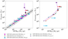 |
Fig. 19. Comparison between the infrared star-formation rates, SFRsIR, and the total and accretion radio luminosities at 150 MHz. Left: SFRsIR of the median quasar samples versus their total radio luminosities at 150 MHz. Error bars on the x-axis indicate 1σ errors on the SFRsIR, while y-axis error bars for LOFAR quasars stacked according to their radio luminosity denotes the bin size used. The dashed line is the far-infrared radio correlation (FIRC) at L150 MHz derived by Calistro-Rivera et al. (2017). The gray shaded region indicates the spread of the FIRC scaled by a factor of ±2. Right: SFRIR versus the radio luminosity associated with AGN accretion, L150MHz, acc. The radio luminosity connected to AGN accretion is calculated by subtracting the contribution of SF to the total radio luminosity estimated using the FIRC. Negative AGN feedback could be taken place in the hosts of RDQs with the highest 150 MHz radio luminosities due to their radio-emission being dominated by AGN accretion, and the relative lower SFRIR. |
While jet-induced star formation could be taking place in the host galaxies of some RDQs as mentioned earlier, it has also been suggested that radio jets could be associated with negative AGN feedback. This either by suppressing gas cooling or by expelling gas from the host galaxy, hence quenching SF in host galaxies. Evidence of gas being expelled by an AGN outflow has been observed in bright radio-galaxies (e.g., Nesvadba et al. 2006). Additionally, Kalfountzou et al. (2017) proposed a model with a jet power threshold that controls radio-jet feedback, where sources with low and intermediate jet powers present SF enhancement, while sources with the highest jet powers above the threshold at which radio-jet feedback changes from positive to negative suppressing SF. Although this model could explain our results for RDQs with L150MHz ≳ 8 × 1026 W Hz−1, other factors such as merger history and environment might influence star formation in the host galaxies of these RDQs.
Finally, it is important to acknowledge that despite the fact that median stacking enables statistical fluxes of undetected sources, it also leads to the lost of information about individual detections. This in the context of the implication that based on AGN feedback, only median trends could be recovered in some cases (i.e., RUQs), while trend outliers where positive or negative AGN feedback could take place have a limited weight in the trends obtained through stacking. Future studies will utilize deeper infrared and radio continuum observations to study a number of open questions regarding AGN feedback without the need to rely on stacking.
7. Conclusions
In this work, we construct the infrared-radio median spectral energy distributions for LOFAR RDQs and RUQs in the NDWFS-Boötes field. To obtain the infrared and radio photometry, we used a stacking analysis of Spitzer, WISE, Herschel, VLA, WSRT, and LOFAR maps. The stacking analysis allows us to probe the radio-emission for quasars that are up to one order of magnitude fainter than the ones detected individually. These results help us to address the questions posed in Sect. 1. We arrive at the following conclusions:
-
The radio-emission of RUQs is consistent to be linked to SF processes, while the radio activity in RDQs is likely associated with accretion onto SMBHs. This is supported by the radio-excess showed by median RDQs with respect to the predictions of the FIRC, while RUQs follow tightly this correlation.
-
The observed behaviour of the radio-loudness parameter, R, is as follows: for bright RDQs with R ≳ −4.5 the radio-emission is consistent with being dominated by SMBH accretion, while for lower-radio luminosity quasars with R < −4.5 the relative contribution of SF to their radio fluxes increases as the SMBH component becomes weaker.
-
For median RDQs, the SMBH accretion can account for ∼50−84% of the total 150 MHz radio luminosity, while for median RUQs the contribution is ∼5−41%. This strongly suggests that vigorous SF activity is coeval with the growth of the SMBHs residing in the nuclei of quasar host galaxies.
-
There is no evidence for the suppression of SF in the host galaxies of median RDQs stacked according to redshift and M1450 (not considering the highest M1450 and z bins where less sources are found). However, when the 150 MHz radio luminosity is considered for the stacking, the highest radio luminosity median RDQs have lower SFRs than median the RDQs with lower radio luminosities. In particular, for the brightest median RDQs at 150 MHz the accretion-related radio luminosity accounts for 97.2% of the total 150 MHz radio luminosity, and has a relative lower SFRIR. This suggests that it is likely that negative AGN feedback has taken place in the hosts of RDQs with the highest 150 MHz radio luminosities in our sample.
-
The spectral indices of median quasars (undetected and detected by LOFAR) do not evolve significantly with redshift, but become flatter towards lower frequencies. Overall, the spectral curvature of RUQs is similar to that of RDQs.
Finally, our results highlight the importance of using deep low- and high- frequency radio surveys to study the properties of RDQs and RUQs, and particularly the radio properties of quasars that generally remain radio silent and hidden in shallow flux-density-limited surveys.
Acknowledgments
ERM acknowledges financial support from NWO Top project, No. 614.001.006. We thank the anonymous referee for the helpful comments that improved this work. LOFAR, the Low Frequency Array designed and constructed by ASTRON, has facilities in several countries, that are owned by various parties (each with their own funding sources), and that are collectively operated by the International LOFAR Telescope (ILT) foundation under a joint scientific policy. The Open University is incorporated by Royal Charter (RC 000391), an exempt charity in England & Wales and a charity registered in Scotland (SC 038302). The Open University is authorized and regulated by the Financial Conduct Authority. Herschel is an ESA space observatory with science instruments provided by European-led Principal Investigator consortia and with important participation from NASA. Herschel/SPIRE has been developed by a consortium of institutes led by Cardiff University (UK) and including Univ. Lethbridge (Canada); NAOC (China); CEA, LAM (France); IFSI, Univ. Padua (Italy); IAC (Spain); Stockholm Observatory (Sweden); Imperial College London, RAL, UCL-MSSL, UKATC, Univ. Sussex (UK); and Caltech, JPL, NHSC, Univ. Colorado (USA). This development has been supported by national funding agencies: CSA (Canada); NAOC (China); CEA, CNES, CNRS (France); ASI (Italy); MCINN (Spain); SNSB (Sweden); STFC, UKSA (UK); and NASA (USA). HIPE is a joint development (are joint developments) by the Herschel Science Ground Segment Consortium, consisting of ESA, the NASA Herschel Science Center, and the HIFI, PACS and SPIRE consortia. This research has made use of data from HerMES project (https://hedam.lam.fr/HerMES/index/survey). HerMES is a Herschel Key Programme utilising Guaranteed Time from the SPIRE instrument team, ESAC scientists and a mission scientist. The HerMES data was accessed through the Herschel Database in Marseille (HeDaM - http://hedam.lam.fr) operated by CeSAM and hosted by the Laboratoire d’Astrophysique de Marseille. The National Radio Astronomy Observatory is a facility of the National Science Foundation operated under cooperative agreement by Associated Universities, Inc. CIRADA is funded by a grant from the Canada Foundation for Innovation 2017 Innovation Fund (Project 35999), as well as by the Provinces of Ontario, British Columbia, Alberta, Manitoba and Quebec. This publication makes use of data products from the Wide-field Infrared Survey Explorer, which is a joint project of the University of California, Los Angeles, and the Jet Propulsion Laboratory/California Institute of Technology, funded by the National Aeronautics and Space Administration.
References
- Alberts, S., Rujopakarn, W., Rieke, G. H., Jagannathan, P., & Nyland, K. 2020, ApJ, 901, 168 [NASA ADS] [CrossRef] [Google Scholar]
- Algera, H. S. B., van der Vlugt, D., Hodge, J. A., et al. 2020, ApJ, 903, 139 [Google Scholar]
- Ashby, M. L. N., Stern, D., Brodwin, M., et al. 2009, ApJ, 701, 428 [Google Scholar]
- Azadi, M., Coil, A. L., Aird, J., et al. 2017, ApJ, 835, 27 [NASA ADS] [CrossRef] [Google Scholar]
- Badole, S., Jackson, N., Hartley, P., et al. 2020, MNRAS, 496, 138 [NASA ADS] [CrossRef] [Google Scholar]
- Baldry, I. K., Driver, S. P., Loveday, J., et al. 2012, MNRAS, 421, 621 [NASA ADS] [Google Scholar]
- Baloković, M., Smolčić, V., Ivezić, Ž., et al. 2012, ApJ, 759, 30 [CrossRef] [Google Scholar]
- Barger, A. J., Cowie, L. L., Chen, C. C., et al. 2014, ApJ, 784, 9 [NASA ADS] [CrossRef] [Google Scholar]
- Becker, R. H., White, R. L., & Helfand, D. J. 1995, ApJ, 450, 559 [Google Scholar]
- Bell, E. F. 2003, ApJ, 586, 794 [Google Scholar]
- Best, P. N., & Heckman, T. M. 2012, MNRAS, 421, 1569 [NASA ADS] [CrossRef] [Google Scholar]
- Best, P. N., Kauffmann, G., Heckman, T. M., et al. 2005, MNRAS, 362, 25 [Google Scholar]
- Bettoni, D., Falomo, R., Kotilainen, J. K., Karhunen, K., & Uslenghi, M. 2015, MNRAS, 454, 4103 [NASA ADS] [CrossRef] [Google Scholar]
- Bian, F., Fan, X., Jiang, L., et al. 2013, ApJ, 774, 28 [Google Scholar]
- Blundell, K. M., Beasley, A. J., Lacy, M., & Garrington, S. T. 1996, ApJ, 468, L91 [NASA ADS] [CrossRef] [Google Scholar]
- Bonfield, D. G., Jarvis, M. J., Hardcastle, M. J., et al. 2011, MNRAS, 416, 13 [NASA ADS] [Google Scholar]
- Bonzini, M., Mainieri, V., Padovani, P., et al. 2015, MNRAS, 453, 1079 [Google Scholar]
- Brown, M. J. I., Dey, A., Jannuzi, B. T., et al. 2007, ApJ, 654, 858 [Google Scholar]
- Calistro-Rivera, G., Williams, W. L., Hardcastle, M. J., et al. 2017, MNRAS, 469, 3468 [Google Scholar]
- Caputi, K. I., Cirasuolo, M., Dunlop, J. S., et al. 2011, MNRAS, 413, 162 [NASA ADS] [CrossRef] [Google Scholar]
- Casey, C. M. 2012, MNRAS, 425, 3094 [Google Scholar]
- Chambers, K. C., Magnier, E. A., Metcalfe, N., et al. 2016, ArXiv e-prints [arXiv:1612.05560] [Google Scholar]
- Cirasuolo, M., Magliocchetti, M., Celotti, A., & Danese, L. 2003, MNRAS, 341, 993 [NASA ADS] [CrossRef] [Google Scholar]
- Condon, J. J. 1992, ARA&A, 30, 575 [Google Scholar]
- Condon, J. J., Cotton, W. D., Greisen, E. W., et al. 1998, AJ, 115, 1693 [Google Scholar]
- Cool, R. J., Kochanek, C. S., Eisenstein, D. J., et al. 2006, AJ, 132, 823 [NASA ADS] [CrossRef] [Google Scholar]
- Coppejans, R., Cseh, D., Williams, W. L., van Velzen, S., & Falcke, H. 2015, MNRAS, 450, 1477 [Google Scholar]
- Croft, S., van Breugel, W., de Vries, W., et al. 2006, ApJ, 647, 1040 [NASA ADS] [CrossRef] [Google Scholar]
- Croom, S. M., Smith, R. J., Boyle, B. J., et al. 2004, MNRAS, 349, 1397 [NASA ADS] [CrossRef] [Google Scholar]
- Daddi, E., Dickinson, M., Morrison, G., et al. 2007, ApJ, 670, 156 [NASA ADS] [CrossRef] [Google Scholar]
- de Vries, W. H., Morganti, R., Röttgering, H. J. A., et al. 2002, AJ, 123, 1784 [Google Scholar]
- Delvecchio, I., Smolčić, V., Zamorani, G., et al. 2017, A&A, 602, A3 [NASA ADS] [CrossRef] [EDP Sciences] [Google Scholar]
- Dey, A., van Breugel, W., Vacca, W. D., & Antonucci, R. 1997, ApJ, 490, 698 [NASA ADS] [CrossRef] [Google Scholar]
- Dong, X. Y., & Wu, X.-B. 2016, ApJ, 824, 70 [NASA ADS] [CrossRef] [Google Scholar]
- Duras, F., Bongiorno, A., Piconcelli, E., et al. 2017, A&A, 604, A67 [NASA ADS] [CrossRef] [EDP Sciences] [Google Scholar]
- Elbaz, D., Dickinson, M., Hwang, H. S., et al. 2011, A&A, 533, A119 [NASA ADS] [CrossRef] [EDP Sciences] [Google Scholar]
- Falder, J. T., Stevens, J. A., Jarvis, M. J., et al. 2010, MNRAS, 405, 347 [NASA ADS] [Google Scholar]
- Falkendal, T., De Breuck, C., Lehnert, M. D., et al. 2019, A&A, 621, A27 [NASA ADS] [CrossRef] [EDP Sciences] [Google Scholar]
- Fanaroff, B. L., & Riley, J. M. 1974, MNRAS, 167, 31P [Google Scholar]
- Fawcett, V. A., Alexander, D. M., Rosario, D. J., et al. 2020, MNRAS, 494, 4802 [Google Scholar]
- Fazio, G. G., Hora, J. L., Allen, L. E., et al. 2004, ApJS, 154, 10 [Google Scholar]
- Feigelson, E. D., & Nelson, P. I. 1985, ApJ, 293, 192 [NASA ADS] [CrossRef] [Google Scholar]
- Flesch, E. W. 2015, PASA, 32 [CrossRef] [Google Scholar]
- Fogasy, J., Knudsen, K. K., Drouart, G., Lagos, C. D. P., & Fan, L. 2020, MNRAS, 493, 3744 [NASA ADS] [CrossRef] [Google Scholar]
- Fu, H., Cooray, A., Feruglio, C., et al. 2013, Nature, 498, 338 [CrossRef] [Google Scholar]
- Gaibler, V., Khochfar, S., Krause, M., & Silk, J. 2012, MNRAS, 425, 438 [NASA ADS] [CrossRef] [Google Scholar]
- Gallagher, S. C., Richards, G. T., Lacy, M., et al. 2007, ApJ, 661, 30 [NASA ADS] [CrossRef] [Google Scholar]
- Garn, T., & Alexander, P. 2009, MNRAS, 394, 105 [NASA ADS] [CrossRef] [Google Scholar]
- Glikman, E., Djorgovski, S. G., Stern, D., et al. 2011, ApJ, 728, L26 [NASA ADS] [CrossRef] [Google Scholar]
- Griffin, M. J., Abergel, A., Abreu, A., et al. 2010, A&A, 518, L3 [EDP Sciences] [Google Scholar]
- Gürkan, G., Hardcastle, M. J., Best, P. N., et al. 2019, A&A, 622, A11 [NASA ADS] [CrossRef] [EDP Sciences] [Google Scholar]
- Hall, K. R., Zakamska, N. L., Addison, G. E., et al. 2019, MNRAS, 490, 2315 [NASA ADS] [CrossRef] [Google Scholar]
- Hardcastle, M. J., Evans, D. A., & Croston, J. H. 2007, MNRAS, 376, 1849 [NASA ADS] [CrossRef] [Google Scholar]
- Harris, K., Farrah, D., Schulz, B., et al. 2016, MNRAS, 457, 4179 [NASA ADS] [CrossRef] [Google Scholar]
- Hartley, P., Jackson, N., Sluse, D., Stacey, H. R., & Vives-Arias, H. 2019, MNRAS, 485, 3009 [Google Scholar]
- Heckman, T. M., & Best, P. N. 2014, ARA&A, 52, 589 [Google Scholar]
- Helou, G., Soifer, B. T., & Rowan-Robinson, M. 1985, ApJ, 298, L7 [Google Scholar]
- Herrera Ruiz, N., Middelberg, E., Norris, R. P., & Maini, A. 2016, A&A, 589, L2 [NASA ADS] [CrossRef] [EDP Sciences] [Google Scholar]
- Hodapp, K. W., Siegmund, W. A., Kaiser, N., et al. 2004, in Groundbased Telescopes, eds. J. Oschmann, & M. Jacobus, SPIE Conf. Ser., 5489, 667 [NASA ADS] [CrossRef] [Google Scholar]
- Hodge, J. A., Becker, R. H., White, R. L., & de Vries, W. H. 2008, AJ, 136, 1097 [Google Scholar]
- Hopkins, P. F., Torrey, P., Faucher-Giguère, C.-A., Quataert, E., & Murray, N. 2016, MNRAS, 458, 816 [NASA ADS] [CrossRef] [Google Scholar]
- Hwang, H. C., Zakamska, N. L., Alexandroff, R. M., et al. 2018, MNRAS, 477, 830 [CrossRef] [Google Scholar]
- Ilbert, O., McCracken, H. J., Le Fèvre, O., et al. 2013, A&A, 556, A55 [NASA ADS] [CrossRef] [EDP Sciences] [Google Scholar]
- Inskip, K. J., Villar-Martín, M., Tadhunter, C. N., et al. 2008, MNRAS, 386, 1797 [NASA ADS] [CrossRef] [Google Scholar]
- Intema, H. T., van Weeren, R. J., Röttgering, H. J. A., & Lal, D. V. 2011, A&A, 535, A38 [NASA ADS] [CrossRef] [EDP Sciences] [Google Scholar]
- Ishibashi, W., & Fabian, A. C. 2012, MNRAS, 427, 2998 [NASA ADS] [CrossRef] [Google Scholar]
- Ivezić, Ž., Menou, K., Knapp, G. R., et al. 2002, AJ, 124, 2364 [CrossRef] [Google Scholar]
- Jannuzi, B. T., & Dey, A. 1999, in Photometric Redshifts and the Detection of High Redshift Galaxies, eds. R. Weymann, L. Storrie-Lombardi, M. Sawicki, & R. Brunner, Astron. Soc. Pacific Conf. Ser., 191, 111 [Google Scholar]
- Jarvis, M. J., Bonfield, D. G., Bruce, V. A., et al. 2013, MNRAS, 428, 1281 [Google Scholar]
- Jiang, L., Fan, X., Ivezić, Ž., et al. 2007, ApJ, 656, 680 [Google Scholar]
- Kalfountzou, E., Stevens, J. A., Jarvis, M. J., et al. 2014, MNRAS, 442, 1181 [NASA ADS] [CrossRef] [Google Scholar]
- Kalfountzou, E., Stevens, J. A., Jarvis, M. J., et al. 2017, MNRAS, 471, 28 [NASA ADS] [CrossRef] [Google Scholar]
- Kellermann, K. I., Sramek, R., Schmidt, M., Shaffer, D. B., & Green, R. 1989, AJ, 98, 1195 [Google Scholar]
- Kennicutt, R. C., Jr 1998, ApJ, 498, 541 [Google Scholar]
- Kimball, A. E., Ivezić, Ž., Wiita, P. J., & Schneider, D. P. 2011, AJ, 141, 182 [NASA ADS] [CrossRef] [Google Scholar]
- Klamer, I. J., Ekers, R. D., Sadler, E. M., & Hunstead, R. W. 2004, ApJ, 612, L97 [NASA ADS] [CrossRef] [Google Scholar]
- Klindt, L., Alexander, D. M., Rosario, D. J., Lusso, E., & Fotopoulou, S. 2019, MNRAS, 488, 3109 [Google Scholar]
- Kochanek, C. S., Eisenstein, D. J., Cool, R. J., et al. 2012, ApJS, 200, 8 [Google Scholar]
- Labbé, I., Huang, J., Franx, M., et al. 2005, ApJ, 624, L81 [Google Scholar]
- Lacy, M., Laurent-Muehleisen, S. A., Ridgway, S. E., Becker, R. H., & White, R. L. 2001, ApJ, 551, L17 [NASA ADS] [CrossRef] [Google Scholar]
- Lacy, M., Baum, S. A., Chandler, C. J., et al. 2020, PASP, 132 [Google Scholar]
- Laor, A., & Behar, E. 2008, MNRAS, 390, 847 [NASA ADS] [CrossRef] [Google Scholar]
- Laor, A., Baldi, R. D., & Behar, E. 2019, MNRAS, 482, 5513 [NASA ADS] [CrossRef] [Google Scholar]
- Leipski, C., Falcke, H., Bennert, N., & Hüttemeister, S. 2006, A&A, 455, 161 [NASA ADS] [CrossRef] [EDP Sciences] [Google Scholar]
- Lutz, D., Mainieri, V., Rafferty, D., et al. 2010, ApJ, 712, 1287 [NASA ADS] [CrossRef] [Google Scholar]
- Magliocchetti, M., Lutz, D., Rosario, D., et al. 2014, MNRAS, 442, 682 [NASA ADS] [CrossRef] [Google Scholar]
- Magliocchetti, M., Lutz, D., Santini, P., et al. 2016, MNRAS, 456, 431 [NASA ADS] [CrossRef] [Google Scholar]
- Magliocchetti, M., Pentericci, L., Cirasuolo, M., et al. 2020, MNRAS, 493, 3838 [Google Scholar]
- Magnelli, B., Ivison, R. J., Lutz, D., et al. 2015, A&A, 573, A45 [NASA ADS] [CrossRef] [EDP Sciences] [Google Scholar]
- Mahony, E. K., Morganti, R., Prandoni, I., et al. 2016, MNRAS, 463, 2997 [Google Scholar]
- Maini, A., Prandoni, I., Norris, R. P., Giovannini, G., & Spitler, L. R. 2016, A&A, 589, L3 [NASA ADS] [CrossRef] [EDP Sciences] [Google Scholar]
- Makovoz, D., Roby, T., Khan, I., & Booth, H. 2006, in SPIE Conf. Ser., eds. H. Lewis, & A. Bridger, 6274, 62740C [NASA ADS] [Google Scholar]
- Matsuoka, Y., Strauss, M. A., Price, T. N., III, & DiDonato, M. S. 2014, ApJ, 780, 162 [Google Scholar]
- Mauch, T., Klöckner, H.-R., Rawlings, S., et al. 2013, MNRAS, 435, 650 [Google Scholar]
- Mauch, T., Cotton, W. D., Condon, J. J., et al. 2020, ApJ, 888, 61 [Google Scholar]
- McGreer, I. D., Becker, R. H., Helfand, D. J., & White, R. L. 2006, ApJ, 652, 157 [Google Scholar]
- Menci, N., Fiore, F., Puccetti, S., & Cavaliere, A. 2008, ApJ, 686, 219 [NASA ADS] [CrossRef] [Google Scholar]
- Miller, L., Peacock, J. A., & Mead, A. R. G. 1990, MNRAS, 244, 207 [NASA ADS] [Google Scholar]
- Miller, P., Rawlings, S., & Saunders, R. 1993, MNRAS, 263, 425 [NASA ADS] [Google Scholar]
- Morabito, L. K., Matthews, J. H., Best, P. N., et al. 2019, A&A, 622, A15 [NASA ADS] [CrossRef] [EDP Sciences] [Google Scholar]
- Mould, J. R., Ridgewell, A., Gallagher, J. S., III, et al. 2000, ApJ, 536, 266 [NASA ADS] [CrossRef] [Google Scholar]
- Nesvadba, N. P. H., Lehnert, M. D., Eisenhauer, F., et al. 2006, ApJ, 650, 693 [NASA ADS] [CrossRef] [Google Scholar]
- Noeske, K. G., Weiner, B. J., Faber, S. M., et al. 2007, ApJ, 660, L43 [CrossRef] [Google Scholar]
- Oke, J. B., & Gunn, J. E. 1983, ApJ, 266, 713 [NASA ADS] [CrossRef] [Google Scholar]
- Oliver, S. J., Bock, J., Altieri, B., et al. 2012, MNRAS, 424, 1614 [NASA ADS] [CrossRef] [Google Scholar]
- Padovani, P. 2016, A&ARv, 24, 13 [Google Scholar]
- Padovani, P., Bonzini, M., Kellermann, K. I., et al. 2015, MNRAS, 452, 1263 [Google Scholar]
- Pâris, I., Petitjean, P., Aubourg, É., et al. 2018, A&A, 613, A51 [Google Scholar]
- Perger, K., Frey, S., Gabányi, K. É., & Tóth, L. V. 2019, MNRAS, 490, 2542 [NASA ADS] [CrossRef] [Google Scholar]
- Pitchford, L. K., Hatziminaoglou, E., Feltre, A., et al. 2016, MNRAS, 462, 4067 [NASA ADS] [CrossRef] [Google Scholar]
- Podigachoski, P., Barthel, P. D., Haas, M., et al. 2015, A&A, 575, A80 [NASA ADS] [CrossRef] [EDP Sciences] [Google Scholar]
- Poglitsch, A., Waelkens, C., Geis, N., et al. 2010, A&A, 518, L2 [NASA ADS] [CrossRef] [EDP Sciences] [Google Scholar]
- Retana-Montenegro, E., & Röttgering, H. 2018, Front. Astron. Space Sci., 5, 5 [NASA ADS] [CrossRef] [Google Scholar]
- Retana-Montenegro, E., & Röttgering, H. J. A. 2017, A&A, 600, A97 [NASA ADS] [CrossRef] [EDP Sciences] [Google Scholar]
- Retana-Montenegro, E., & Röttgering, H. 2020, A&A, 636, A12 [NASA ADS] [CrossRef] [EDP Sciences] [Google Scholar]
- Retana-Montenegro, E., Röttgering, H. J. A., Shimwell, T. W., et al. 2018, A&A, 620, A74 [NASA ADS] [CrossRef] [EDP Sciences] [Google Scholar]
- Richards, G. T., Fan, X., Schneider, D. P., et al. 2001, AJ, 121, 2308 [NASA ADS] [CrossRef] [Google Scholar]
- Richards, G. T., Lacy, M., Storrie-Lombardi, L. J., et al. 2006, ApJS, 166, 470 [Google Scholar]
- Riechers, D. A., Carilli, C. L., Maddalena, R. J., et al. 2011, ApJ, 739, L32 [CrossRef] [Google Scholar]
- Rieke, G. H., Young, E. T., Engelbracht, C. W., et al. 2004, ApJS, 154, 25 [Google Scholar]
- Rosario, D. J., Trakhtenbrot, B., Lutz, D., et al. 2013, A&A, 560, A72 [NASA ADS] [CrossRef] [EDP Sciences] [Google Scholar]
- Rosario, D. J., Fawcett, V. A., Klindt, L., et al. 2020, MNRAS, 494, 3061 [Google Scholar]
- Roseboom, I. G., Oliver, S. J., Kunz, M., et al. 2010, MNRAS, 409, 48 [Google Scholar]
- Rovilos, E., Comastri, A., Gilli, R., et al. 2012, A&A, 546, A58 [NASA ADS] [CrossRef] [EDP Sciences] [Google Scholar]
- Salomé, Q., Salomé, P., Miville-Deschênes, M. A., Combes, F., & Hamer, S. 2017, A&A, 608, A98 [NASA ADS] [CrossRef] [EDP Sciences] [Google Scholar]
- Sanders, D. B., Salvato, M., Aussel, H., et al. 2007, ApJS, 172, 86 [Google Scholar]
- Santini, P., Fontana, A., Grazian, A., et al. 2009, A&A, 504, 751 [NASA ADS] [CrossRef] [EDP Sciences] [Google Scholar]
- Santini, P., Fontana, A., Castellano, M., et al. 2017, ApJ, 847, 76 [NASA ADS] [CrossRef] [Google Scholar]
- Scaife, A. M. M., & Heald, G. H. 2012, MNRAS, 423, L30 [Google Scholar]
- Schlafly, E. F., & Finkbeiner, D. P. 2011, ApJ, 737, 103 [Google Scholar]
- Schmidt, M. 1963, Nature, 197, 1040 [Google Scholar]
- Schneider, D. P., Hall, P. B., Richards, G. T., et al. 2005, AJ, 130, 367 [NASA ADS] [CrossRef] [Google Scholar]
- Scholtz, J., Alexander, D. M., Harrison, C. M., et al. 2018, MNRAS, 475, 1288 [NASA ADS] [CrossRef] [Google Scholar]
- Schreiber, C., Pannella, M., Elbaz, D., et al. 2015, A&A, 575, A74 [NASA ADS] [CrossRef] [EDP Sciences] [Google Scholar]
- Schulze, A., Silverman, J. D., Daddi, E., et al. 2019, MNRAS, 488, 1180 [NASA ADS] [CrossRef] [Google Scholar]
- Serjeant, S., & Hatziminaoglou, E. 2009, MNRAS, 397, 265 [NASA ADS] [CrossRef] [Google Scholar]
- Seymour, N., Symeonidis, M., Page, M. J., et al. 2011, MNRAS, 413, 1777 [NASA ADS] [CrossRef] [Google Scholar]
- Shangguan, J., Ho, L. C., Bauer, F. E., Wang, R., & Treister, E. 2020, ApJS, 247, 15 [NASA ADS] [CrossRef] [Google Scholar]
- Singal, J., Petrosian, V., Lawrence, A., & Stawarz, L. 2011, ApJ, 743, 104 [NASA ADS] [CrossRef] [Google Scholar]
- Sirothia, S. K., Dennefeld, M., Saikia, D. J., et al. 2009, MNRAS, 395, 269 [Google Scholar]
- Smolčić, V. 2009, ApJ, 699, L43 [Google Scholar]
- Smolčić, V., Novak, M., Bondi, M., et al. 2017, A&A, 602, A1 [Google Scholar]
- Sopp, H. M., & Alexander, P. 1991, MNRAS, 251, 112 [NASA ADS] [CrossRef] [Google Scholar]
- Speagle, J. S., Steinhardt, C. L., Capak, P. L., & Silverman, J. D. 2014, ApJS, 214, 15 [Google Scholar]
- Stanley, F., Harrison, C. M., Alexander, D. M., et al. 2015, MNRAS, 453, 591 [Google Scholar]
- Stanley, F., Alexander, D. M., Harrison, C. M., et al. 2017, MNRAS, 472, 2221 [Google Scholar]
- Steinhardt, C. L., Speagle, J. S., Capak, P., et al. 2014, ApJ, 791, L25 [Google Scholar]
- Terlevich, R. J., & Boyle, B. J. 1993, MNRAS, 262, 491 [NASA ADS] [CrossRef] [Google Scholar]
- Trakhtenbrot, B., Lira, P., Netzer, H., et al. 2017, ApJ, 836, 8 [NASA ADS] [CrossRef] [Google Scholar]
- Ulvestad, J. S., Antonucci, R. R. J., & Barvainis, R. 2005, ApJ, 621, 123 [Google Scholar]
- van Breugel, W., Fragile, C., Anninos, P., & Murray, S. 2004, in Recycling Intergalactic and Interstellar Matter, eds. P.-A. Duc, J. Braine, & E. Brinks, IAU Symp., 217, 472 [NASA ADS] [Google Scholar]
- van Haarlem, M. P., Wise, M. W., Gunst, A. W., et al. 2013, A&A, 556, A2 [NASA ADS] [CrossRef] [EDP Sciences] [Google Scholar]
- van Weeren, R. J., Williams, W. L., Tasse, C., et al. 2014, ApJ, 793, 82 [Google Scholar]
- Venemans, B. P., Röttgering, H. J. A., Miley, G. K., et al. 2007, A&A, 461, 823 [NASA ADS] [CrossRef] [EDP Sciences] [Google Scholar]
- Viero, M. P., Moncelsi, L., Quadri, R. F., et al. 2015, ApJ, 809, L22 [NASA ADS] [CrossRef] [Google Scholar]
- Wals, M., Boyle, B. J., Croom, S. M., et al. 2005, MNRAS, 360, 453 [NASA ADS] [CrossRef] [Google Scholar]
- Wardlow, J. L., Smail, I., Coppin, K. E. K., et al. 2011, MNRAS, 415, 1479 [Google Scholar]
- Whitaker, K. E., van Dokkum, P. G., Brammer, G., & Franx, M. 2012, ApJ, 754, L29 [Google Scholar]
- White, R. L., Helfand, D. J., Becker, R. H., Glikman, E., & deVries, W. 2007, ApJ, 654, 99 [NASA ADS] [CrossRef] [Google Scholar]
- White, S. V., Jarvis, M. J., Häußler, B., & Maddox, N. 2015, MNRAS, 448, 2665 [Google Scholar]
- White, S. V., Jarvis, M. J., Kalfountzou, E., et al. 2017, MNRAS, 468, 217 [Google Scholar]
- Williams, W. L., Intema, H. T., & Röttgering, H. J. A. 2013, A&A, 549, A55 [NASA ADS] [CrossRef] [EDP Sciences] [Google Scholar]
- Williams, W. L., van Weeren, R. J., Röttgering, H. J. A., et al. 2016, MNRAS, 460, 2385 [Google Scholar]
- Wright, E. L., Eisenhardt, P. R. M., Mainzer, A. K., et al. 2010, AJ, 140, 1868 [Google Scholar]
- Yao, S., Wu, X.-B., Ai, Y. L., et al. 2019, ApJS, 240, 6 [NASA ADS] [CrossRef] [Google Scholar]
- Yue, M., Jiang, L., Shen, Y., et al. 2018, ApJ, 863, 21 [NASA ADS] [CrossRef] [Google Scholar]
- Yun, M. S., Reddy, N. A., & Condon, J. J. 2001, ApJ, 554, 803 [Google Scholar]
- Zakamska, N. L., & Greene, J. E. 2014, MNRAS, 442, 784 [Google Scholar]
- Zakamska, N. L., Lampayan, K., Petric, A., et al. 2016, MNRAS, 455, 4191 [Google Scholar]
- Zhang, Y., Dietrich, J. P., McKay, T. A., Sheldon, E. S., & Nguyen, A. T. Q. 2013, ApJ, 773, 115 [NASA ADS] [CrossRef] [Google Scholar]
- Zubovas, K., & King, A. 2012, ApJ, 745, L34 [Google Scholar]
Appendix A: Median-stacked infrared and radio maps of LOFAR radio-detected and LOFAR radio-undetected quasars
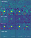 |
Fig. A.1. Central area of the median stacked infrared maps (IRAC, WISE, MIPS, and PACS) of LOFAR radio-undetected quasars. The number of quasars stacked in each is indicated in Table 3. The size of the maps is 80″ × 80. The corresponding synthesized beam size is indicated in the left corner. The color scale ranges from −3σL to 5σL , where σL is the local rms noise. |
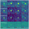 |
Fig. A.2. Central area of the median stacked infrared maps (PACS, and SPIRE) of LOFAR radio-undetected quasars. The number of quasars stacked in each is indicated in Table 3. The size of the maps is 125″ × 125″. The corresponding synthesized beam size is indicated in the left corner. The color scale varies from −3σL to 5σL , where σL is the local rms noise. |
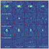 |
Fig. A.3. Central area of the median stacked radio maps of LOFAR radio-undetected quasars. The number of quasars stacked in each is indicated in Table 3. The size of the maps is 25″ × 25″, except the WSRT map which has a size of 80″ × 80″. The corresponding synthesized beam size is indicated in the left corner. The color scale varies from −5σL to 15σL , where σL is the local rms noise. The contours are drawn at [3, 4, 5, 10]×σL times the local rms noise level. |
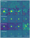 |
Fig. A.4. Central area of the median stacked infrared maps (IRAC, WISE, MIPS, and PACS) of LOFAR radio-detected quasars. The number of quasars stacked in each is indicated in Table 3. The size of the maps is 80″ × 80. The corresponding synthesized beam size is indicated in the left corner. The color scale ranges from −3σL to 5σL , where σL is the local rms noise. |
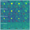 |
Fig. A.5. Central area of the median stacked infrared maps (PACS, SPIRE) of LOFAR radio-detected quasars. The number of quasars stacked in each is indicated in Table 3.. The size of the maps is 125″ × 125″. The corresponding synthesized beam size is indicated in the left corner. The color scale ranges from −3σL to 5σL , where σL is the local rms noise. |
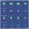 |
Fig. A.6. Central area of the median stacked radio maps of LOFAR radio-detected quasars. The number of quasars stacked in each is indicated in Table 3. The size of the maps is 25″ × 25″, except the WSRT map which has a size of 80″ × 80″. The corresponding synthesized beam size is indicated in the left corner. The color scale ranges from −5σL to 15σL , where σL is the local rms noise. |
Appendix B: Infrared photometry of median LOFAR radio-detected and LOFAR radio-undetected quasars stacked according to redshift
Infrared fluxes of the median LOFAR radio-detected quasars (RDQs) and LOFAR radio-undetected quasars (RUQs) stacked according to redshift between 8μm and 500μm. Values without error bars are upper limits estimated at the center of the median stacked images.
All Tables
Radio fluxes of the median LOFAR radio-detected quasars (RDQs) and LOFAR radio-undetected quasars (RUQs) stacked according to redshift between 150 MHz and 3.0 GHz.
Noise levels (1σ) of the median radio images stacked according to redshift of LOFAR radio-detected quasars (RDQs) and LOFAR radio-undetected quasars (RUQs).
Infrared fluxes of the median LOFAR radio-detected quasars (RDQs) and LOFAR radio-undetected quasars (RUQs) stacked according to redshift between 8μm and 500μm. Values without error bars are upper limits estimated at the center of the median stacked images.
All Figures
|
Fig. 1. Footprints of the various surveys of the NDWFS-Boötes field used in this work. The beam size for each instrument is also indicated. The 3.0 GHz VLASS observations overlap with the LOFAR region. The analysis in this work is limited to the region with WSRT coverage. |
| In the text | |
|
Fig. 2. Total flux S150 MHz distributions of LOFAR radio-detected quasars. |
| In the text | |
|
Fig. 3. Maximum-value normalized I-band distributions of LOFAR radio-detected quasars (RDQs, red) and LOFAR radio-undetected quasars (RUQs, blue). Also, the total combined redshift distribution of RDQs and RUQs (black) is plotted. |
| In the text | |
|
Fig. 4. Absolute magnitude at rest-frame 1450 Å, M1450, versus redshift for the LOFAR radio-detected quasars (red) and LOFAR radio-undetected quasars (blue) samples. The dashed line denotes the magnitude limit iPS = 23.0. This limit is calculated assuming a quasar continuum described by a power-law with slope α = −0.5, and with no emission line contribution or Lyα forest blanketing. |
| In the text | |
|
Fig. 5. Rest-frame radio luminosity density at 150 MHz versus redshift for LOFAR radio-detected quasars (red) in our sample. The green (LOFAR radio-detected quasars) and gray squares (LOFAR radio-undetected quasars) are the radio luminosities obtained from the stacking analysis in Sect. 4.1. The dashed line denotes the 5σ flux limit (275 μJy) of the NDWFS-Boötes observations presented by Retana-Montenegro et al. (2018). The stacking analysis allows us to probe the radio-luminosity for quasars that are up to one order of magnitude fainter than the ones detected individually. |
| In the text | |
|
Fig. 6. Normalized absolute magnitude M1450 distributions of LOFAR radio-detected quasars (RDQs, red) and LOFAR radio-undetected quasars (RUQs, blue). Also, the combined redshift distribution of RDQs and RUQs (black) is plotted. The median M1450 values of the samples are indicated by the dashed lines. |
| In the text | |
|
Fig. 7. Median-stacked 150 MHz flux densities versus redshift for all LOFAR radio-undetected quasars (RUQs) in our sample, and for RUQs with M1450 ≤ −23.0. The samples follow similar trends, indicating that selection effects could be present in both samples. |
| In the text | |
|
Fig. 8. Rest-frame spectral energy distributions (SEDs) for median LOFAR radio-undetected quasars stacked according to redshift. Black points plot the observed flux densities with downward-pointing fuchsia arrows indicating 5σ upper limits. The solid blue line shows the combined best-fit SED model, while the purple, green and orange lines show the synchrotron, black-body, and AGN best-fit components, respectively. The maroon squares indicate the predicted fluxes according to the fitted SED model. The cyan points denote the fluxes of the quasars used in the stacking. Some quasars have WSRT and VLA detections, but remain undetected in LOFAR, thus are classified as RUQS. See Sect. 3 for more details. |
| In the text | |
|
Fig. 9. Rest-frame spectral energy distributions (SEDs) for median LOFAR radio-detected quasars stacked according to redshift. Black points plot the observed flux densities with downward-pointing fuchsia arrows indicating 5σ upper limits. The solid blue line shows the combined best-fit SED model, while the purple, green and orange lines show the synchrotron, black-body, and AGN best-fit components, respectively. The maroon squares indicate the predicted fluxes according to the fitted SED model. The cyan points denote the fluxes of the quasars used in the stacking. |
| In the text | |
|
Fig. 10. Comparison between infrared luminosity, LIR, and radio luminosity at 150 MHz and 1400 MHz. Left: LIR versus the radio luminosity at 150 MHz. LIR and L150 MHz are in units of solar luminosity. Measurements for median LOFAR radio-undetected quasars (RUQs, fuchsia and cyan squares), median LOFAR radio-detected quasars (RDQs, red and turquoise stars), RDQs detected by SPIRE at 250 μm (maroon stars), RUQs detected by SPIRE at 250 μm (yellow circles), and RUQs undetected by SPIRE at 250 μm (green circles) are shown. Upper limits are indicated by arrows in either LIR or L150 MHz. For median quasars, the increasing symbol size indicates an the increment in redshift or M1450 absolute luminosity. The dashed line is the far-infrared radio correlation (FIRC) at L150 MHz derived by Calistro-Rivera et al. (2017). The gray shaded region indicates the spread of the FIRC scaled by a factor of ±2. The text indicates the median redshift of the first and last redshift bins of the stacking according to redshift. Right: Same as the right panel, but for the radio luminosity at 1400 MHz, L1400 MHz. Measurements for RUQs detected by WSRT, but undetected by SPIRE at 250 μm (purple circles); and RUQs detected by both SPIRE and WSRT at 250 μm and 1400 MHz (blue circles), respectively are also displayed. |
| In the text | |
|
Fig. 11. Comparison between star-formation rates (SFRs) derived using infrared and radio data. Left: SFR derived from the infrared luminosity, SFRIR, versus the SFR derived from the radio luminosity at 150 MHz. SFRIR and SFR150 MHz are in units of solar mass per year. The measurements for median LOFAR radio-undetected quasars (RUQs) (fuchsia and cyan squares), RUQs detected by SPIRE at 250 μm (yellow circles), and RUQs undetected by SPIRE at 250 μm (green circles) are showed. Upper limits are indicated by arrows in either SFRIR or SFR150 MHz. For median quasars, the increasing symbol size indicates an increment in the redshift or M1450 absolute luminosity. The dashed line is the far-infrared radio correlation (FIRC) at L150 MHz derived by Calistro-Rivera et al. (2017). The gray shaded region indicates the spread of the FIRC scaled by a factor of ±2. The text indicates the median redshift of the first and last redshift bins of the stacking according to redshift. Right: Same as the right panel, but for the SFR at 1400 MHz, SFR1400 MHz. The measurements for RUQs detected by WSRT, but undetected by SPIRE at 250 μm (purple circles); and RUQs detected by both SPIRE and WSRT at 250 μm and 1400 MHz (blue circles), respectively are also displayed. |
| In the text | |
|
Fig. 12. Infrared star formation rate (SFR) distribution for the RDQs and RUQs derived from the infrared luminosity LIR with ≥2σ SPIRE-250 μm detections. The mean SFR of the samples are indicated by the dashed lines. The mean SFRs of our quasar samples are consistent with those of the main sequence star-forming galaxies. |
| In the text | |
|
Fig. 13. Infrared star formation rate (SFRIR) of LOFAR radio-detected quasars (RDQs) and LOFAR radio-undetected quasars (RUQs) versus redshift. The filled stars and squares and associated vertical error bars show the median value in each bin. The horizontal error bars indicate the extend of the redshift bins used. The marron stars and cyan squares show the results for the RDQs and RUQs, respectively, with ≥ 2σ SPIRE-250 μm detections. The solid lines represent the predicted SFRs as a function of redshift derived for the median quasars using the star-formation main sequence (SFMS) relation by Schreiber et al. (2015). The cyan and orange shaded regions indicate the uncertainty intervals of the fitting provided by Schreiber et al. (2015). The vertical errror bars indicate the errors of the SFRIR estimates obtained using the SED fitting, while the horizontal errors indicate the size of the redshift intervals considered. There is a good agreement between the measured median SFRIR for RDQs and RUQs, and the SFMS predictions considering the width of the redshift bins employed and the intrinsic scatter of the SFMS relation. |
| In the text | |
|
Fig. 14. Infrared star-formation rates (SFRsIR) versus absolute magnitude at 1450 Å, M1450, (top panel) and 150 MHz radio luminosity (bottom panel) for LOFAR radio-detected quasars (RDQs) and radio-undetected quasars (RUQs). Only RDQs (stars) and RUQs (squares) with ≥ 2σ SPIRE-250 μm detections are shown (see Sect. 2.3). For median quasars, the increasing symbol size indicates an increment in the redshift, M1450 absolute luminosity, or 150 MHz radio luminosity. The errors on the horizontal axis indicate the extend of the luminosity bins used. Vertical error bars are the 1σ uncertainties for the SFRsIR obtained from the SED fitting. The positive correlation between optical and radio luminosities suggest that there is a link between their SFR and AGN activity in median RDQs and RUQs, with indications of star formation being suppressed in the host galaxies of the most luminous radio quasars. |
| In the text | |
|
Fig. 15. Evolution of spectral indexes α3.0−1.4 (top), α1400−325 (middle), and α325−150 (bottom) as a function of redshift for LOFAR radio-detected quasars (RDQs). The purple circles represent the median RDQs; green circles are the RDQs detected at both frequencies; yellow or red circles indicated RDQs that are undetected in the upper or lower frequency, respectively; and blue circles are RDQs undetected at both frequencies. The horizontal dashed line indicates the canonical value of α = −0.7. |
| In the text | |
|
Fig. 16. Evolution of spectral indexes α3.0−1.4 (top), α1400−325 (middle), and α325−150 (bottom) as a function of redshift for LOFAR radio-undetected quasars (RUQs). The purple circles represent the median RUQs; green circles are the RUQs detected at both frequencies; yellow or red circles indicated RUQs that are undetected in the upper or lower frequency, respectively; and blue circles are RUQs undetected at both frequencies. The horizontal dashed line indicates the canonical value of α = −0.7. |
| In the text | |
|
Fig. 17. Infrared star formation luminosity, LSF, versus radio-loudness, R, for the quasar samples. The measurements for median LOFAR radio-undetected quasars (RUQs, fuchsia squares), median LOFAR radio-undetected quasars (RDQs, red stars), RDQs (maroon stars) and RUQs detected by SPIRE at 250 μm (orange circles), and RUQs undetected by SPIRE and WSRT at 250 μm and 1.4 GHz (green circles), respectively. The measurements for RUQs detected by WSRT, but undetected by SPIRE at 250 μm (purple circles, right); and RUQs detected by both SPIRE and WSRT at 250 μm and 1.4 GHz (blue circles, right), respectively are also displayed. Upper limits in either LSF or L150 MHz are indicated by arrows. The solid line is the far-infrared radio correlation (FIRC) at 150 MHz and 1.4 GHz. The gray shaded region indicates the spread of the FIRC scaled by a factor of ±2. The dashed vertical lines (R = −4.5 at 150 MHz and R = −4.2 at 1.4 GHz) denote the threshold between radio-loud and radio-quiet quasars (see Sect. 6 for more details). The radio-emission of bright RDQs with R ≳ −4.5 is consistent with being dominated by SMBH accretion, while for lower radio luminosity quasars with R < −4.5 the relative contribution of SF to their radio fluxes becomes more important. |
| In the text | |
|
Fig. 18. Distributions of the radio-loudness parameter, R, derived using the 150 MHz radio luminosity for different LOFAR radio-detected quasar (RDQs) samples. The means of each distribution is indicated by the corresponding dashed line. |
| In the text | |
|
Fig. 19. Comparison between the infrared star-formation rates, SFRsIR, and the total and accretion radio luminosities at 150 MHz. Left: SFRsIR of the median quasar samples versus their total radio luminosities at 150 MHz. Error bars on the x-axis indicate 1σ errors on the SFRsIR, while y-axis error bars for LOFAR quasars stacked according to their radio luminosity denotes the bin size used. The dashed line is the far-infrared radio correlation (FIRC) at L150 MHz derived by Calistro-Rivera et al. (2017). The gray shaded region indicates the spread of the FIRC scaled by a factor of ±2. Right: SFRIR versus the radio luminosity associated with AGN accretion, L150MHz, acc. The radio luminosity connected to AGN accretion is calculated by subtracting the contribution of SF to the total radio luminosity estimated using the FIRC. Negative AGN feedback could be taken place in the hosts of RDQs with the highest 150 MHz radio luminosities due to their radio-emission being dominated by AGN accretion, and the relative lower SFRIR. |
| In the text | |
|
Fig. A.1. Central area of the median stacked infrared maps (IRAC, WISE, MIPS, and PACS) of LOFAR radio-undetected quasars. The number of quasars stacked in each is indicated in Table 3. The size of the maps is 80″ × 80. The corresponding synthesized beam size is indicated in the left corner. The color scale ranges from −3σL to 5σL , where σL is the local rms noise. |
| In the text | |
|
Fig. A.2. Central area of the median stacked infrared maps (PACS, and SPIRE) of LOFAR radio-undetected quasars. The number of quasars stacked in each is indicated in Table 3. The size of the maps is 125″ × 125″. The corresponding synthesized beam size is indicated in the left corner. The color scale varies from −3σL to 5σL , where σL is the local rms noise. |
| In the text | |
|
Fig. A.3. Central area of the median stacked radio maps of LOFAR radio-undetected quasars. The number of quasars stacked in each is indicated in Table 3. The size of the maps is 25″ × 25″, except the WSRT map which has a size of 80″ × 80″. The corresponding synthesized beam size is indicated in the left corner. The color scale varies from −5σL to 15σL , where σL is the local rms noise. The contours are drawn at [3, 4, 5, 10]×σL times the local rms noise level. |
| In the text | |
|
Fig. A.4. Central area of the median stacked infrared maps (IRAC, WISE, MIPS, and PACS) of LOFAR radio-detected quasars. The number of quasars stacked in each is indicated in Table 3. The size of the maps is 80″ × 80. The corresponding synthesized beam size is indicated in the left corner. The color scale ranges from −3σL to 5σL , where σL is the local rms noise. |
| In the text | |
|
Fig. A.5. Central area of the median stacked infrared maps (PACS, SPIRE) of LOFAR radio-detected quasars. The number of quasars stacked in each is indicated in Table 3.. The size of the maps is 125″ × 125″. The corresponding synthesized beam size is indicated in the left corner. The color scale ranges from −3σL to 5σL , where σL is the local rms noise. |
| In the text | |
|
Fig. A.6. Central area of the median stacked radio maps of LOFAR radio-detected quasars. The number of quasars stacked in each is indicated in Table 3. The size of the maps is 25″ × 25″, except the WSRT map which has a size of 80″ × 80″. The corresponding synthesized beam size is indicated in the left corner. The color scale ranges from −5σL to 15σL , where σL is the local rms noise. |
| In the text | |
Current usage metrics show cumulative count of Article Views (full-text article views including HTML views, PDF and ePub downloads, according to the available data) and Abstracts Views on Vision4Press platform.
Data correspond to usage on the plateform after 2015. The current usage metrics is available 48-96 hours after online publication and is updated daily on week days.
Initial download of the metrics may take a while.