| Issue |
A&A
Volume 668, December 2022
|
|
|---|---|---|
| Article Number | A54 | |
| Number of page(s) | 19 | |
| Section | Extragalactic astronomy | |
| DOI | https://doi.org/10.1051/0004-6361/202244072 | |
| Published online | 01 December 2022 | |
Probing the megaparsec-scale environment of hyperluminous infrared galaxies at 2 < z < 4
1
Kapteyn Astronomical Institute, University of Groningen, Postbus 800, 9700 AV Groningen, The Netherlands
e-mail: This email address is being protected from spambots. You need JavaScript enabled to view it.
2
SRON Netherlands Institute for Space Research, Landleven 12, 9747 AD Groningen, The Netherlands
3
Imperial College London, Blackett Laboratory, Prince Consort Road, London SW7 2AZ, UK
4
Department of Physics and Astronomy, University of Hawai’i, 2505 Correa Road, Honolulu, HI 96822, USA
5
Institute for Astronomy, 2680 Woodlawn Drive, University of Hawai’i, Honolulu, HI 96822, USA
6
Department of Space and Astronautical Science, Graduate University for Advanced Studies, SOKENDAI, Shonankokusaimura, Hayama, Miura District, Kanagawa 240-0193, Japan
7
Institute of Space and Astronautical Science, Japan Aerospace Exploration Agency, 3-1-1 Yoshinodai, Chuo-ku, Sagamihara, Kanagawa 252-5210, Japan
Received:
20
May
2022
Accepted:
2
September
2022
Abstract
Context. Protoclusters are progenitors of galaxy clusters and they serve as an important key in studies of how halo mass and stellar mass assemble in the early universe. Finding the signposts of such overdense regions, such as bright dusty star-forming galaxies (DSFG), is a popular method for identifying protocluster candidates.
Aims. Hyperluminous infrared galaxies (HLIRGs) are ultramassive and show extreme levels of dusty star formation and black hole accretion that are expected to reside in overdense regions with massive halos. We study the megaparsec-scale environment of the largest HLIRG sample to date (526 HLIRGs over 26 deg2) and we investigate whether they are, in fact, predominantly located in overdense regions.
Methods. We first explored the surface density of Herschel 250 μm sources around HLIRGs and made comparisons with the corresponding values around random positions. Then, we compared the spatial distribution of neighbors around HLIRGs with their counterparts around randomly selected galaxies using a deep IRAC-selected catalog with good-quality photometric redshifts. We also used a redshift-matched quasar sample and submillimeter galaxy (SMG) sample to validate our method, as previous clustering studies have measured the host halo masses of these populations. Finally, we adopted a friends of friends (FoF) algorithm to look for (proto)clusters hosting HLIRGs.
Results. We find that HLIRGs tend to have more bright star-forming neighbors (with 250 μm flux density > 10 mJy) within a 100″ projected radius (∼0.8 Mpc at 2 < z < 4), as compared to a random galaxy at a 3.7σ significance. In our 3D analysis, we find relatively weak excess of IRAC-selected sources within 3 Mpc around HLIRGs compared with random galaxy neighbors, mainly influenced by photometric redshift uncertainty and survey depth. We find a more significant difference (at a 4.7σ significance) in the number of Low Frequency Array (LOFAR)-detected neighbors in the deepest ELAIS-N1 (EN1) field. Furthermore, HLIRGs at 3 < z < 4 show stronger excess compared to HLIRGs at 2 < z < 3 (0.13 ± 0.04 and 0.14 ± 0.01 neighbors around HLIRGs and random positions at 2 < z < 3, respectively, and 0.08 ± 0.04 and 0.05 ± 0.01 neighbors around HLIRGs and random positions at 3 < z < 4, respectively), which is consistent with cosmic downsizing. Finally, we present a list of 30 of the most promising protocluster candidates selected for future follow-up observations.
Key words: galaxies: clusters: general / galaxies: groups: general / galaxies: high-redshift
© F. Gao et al. 2022
 Open Access article, published by EDP Sciences, under the terms of the Creative Commons Attribution License (https://creativecommons.org/licenses/by/4.0), which permits unrestricted use, distribution, and reproduction in any medium, provided the original work is properly cited.
This article is published in open access under the Subscribe-to-Open model. This email address is being protected from spambots. You need JavaScript enabled to view it. to support open access publication.
1. Introduction
In the local Universe, the morphology-density relation has been well established: Galaxies that reside in dense regions such as clusters are more likely to be massive ellipticals and have lower star formation rates (SFR), while galaxies in less crowded regions are more likely to be less massive spirals with ongoing star formation (Dressler 1980; Lewis et al. 2002; Gómez et al. 2003; Kauffmann et al. 2004; Thomas et al. 2005; Peng et al. 2010; Cappellari et al. 2011; Scoville et al. 2013). Numerous studies have also revealed that massive early-type galaxies formed most of their stellar mass in the early universe (galaxy downsizing, e.g., Cowie et al. 1996; Thomas et al. 2005; De Lucia et al. 2006; Cimatti et al. 2008; Pérez-González et al. 2008; Ilbert et al. 2010). Therefore, overdense regions at the present day such as galaxy clusters that host massive early-type galaxies must have had rapid star-formation activity at higher redshifts, when clusters are less virialized (often referred as protoclusters; Overzier 2016). For example, Elbaz et al. (2007) used data from the Great Observatories Origins Deep Survey (GOODS) and demonstrated that SFR increases as galaxy density increases at z ∼ 1, contrary to what have been found for local galaxies. By studying galaxy members in a Spitzer-selected cluster at z = 1.62, Tran et al. (2010) found that the fraction of star-forming galaxies (SFGs) triples from the lowest to the highest density regions. A recent work by Lemaux et al. (2022), which studied 6730 spectroscopically confirmed SFGs at 2 < z < 5 found a positive trend between average SFR and local environment.
Protoclusters are progenitors of today’s most massive structures. They play an important role in answering many key questions, such as how halo and stellar mass assemble across cosmic time, how environment affects the evolution of massive galaxies, and so on. To study the nature of protoclusters, we first need an efficient method to find them. However, identifying protoclusters is more challenging than identifying their descendant clusters, which can be found by searching for overdensity of red massive galaxies or hot intracluster medium (ICM) through the Sunyaev–Zel’Dovich effect. In contrast, the lack of red massive galaxies and mature ICM make it difficult to trace protoclusters (see review Overzier 2016, and references therein).
By definition, protoclusters can be selected by tracing overdensity of galaxies in a small region (on the scale corresponding to the expected size of massive halos scale of several Mpc), which would ideally be spectroscopically confirmed. However, good-quality photometric redshifts have also been used (e.g., Capak et al. 2011; Chiang et al. 2014; Franck & McGaugh 2016; Lemaux et al. 2018). An alternative method is to trace the surface overdensity of galaxies that occupy a narrow redshift slice. For example, Lee et al. (2014) reported a large-scale structure containing three protoclusters at z = 3.78 in the Boötes field by searching for an overdensity of Lyman α emitter (LAE) candidates. In their work, a deep imaging survey revealed 65 LAEs within a comoving volume of 72 × 72 × 25 Mpc3. These protoclusters may evolve into clusters with a total stellar mass of a few times of 1014 M⊙ to 1015 M⊙ at the present day. Toshikawa et al. (2018) selected 179 protocluster candidates at z ∼ 4 by tracing surface overdensity of Lyman break galaxies (LBGs), based on data from the Hyper SuprimeCam Subaru strategic program (HSC-SSP) covering a wide area of 121 deg2. These methods provide a simple and direct way to identify potential protoclusters, thus contributing to a population census of protoclusters. However, they usually require a large-area sky survey to conduct a systematic search for overdense regions due to their rarity. Moreover, as redshift increases, protoclusters occupying a given volume will cover a larger sky area, making it more challenging to find them in a survey with limited sky coverage. In addition, selections based on overdensities of LAEs or LBGs may not be able to uncover overdensities of dusty star-forming galaxies which dominate the star-forming population at high redshifts (e.g., see Casey et al. 2014, for a review) due to severe obscuration in the optical bands. Owing to these difficulties, identification of protoclusters at high redshifts is so far largely dependent on serendipitous findings, by targeting signposts which are expected to reside in dense regions. Popular signposts include radio-loud galaxies (e.g., Pentericci et al. 2000; Kurk et al. 2001; Hayashi et al. 2012; Shimakawa et al. 2014), enormous Lyman α nebulae (e.g., Arrigoni Battaia et al. 2018; Cai et al. 2018; Li et al. 2021; Nowotka et al. 2022) and quasars (e.g., Steidel et al. 2005; Balmaverde et al. 2017; García-Vergara et al. 2022).
Given the fact that larger SFR is observed in denser region at high redshifts and the predominant role of dusty star-formation activity at high redshifts, it is widely adopted in the search for protoclusters either through overdensities of dusty star-forming galaxies (DSFGs) or using bright DSFGs as a signpost. DSFG can be selected as bright far-infrared (FIR) or submillimeter detections. Their star formation activity is obscured by dust which absorbs UV/optical photons and re-emits them in the longer wavelength range. One efficient method to find overdensity of DSFGs is using large FIR/submillimeter surveys covering a wide area such as surveys with Planck and Herschel. The total flux density within the beam of a low-resolution instrument is usually a combination of multiple sources located within the same beam. Follow-up high-resolution imaging can help confirm the overdense nature for regions with exceedingly large flux densities (e.g., Negrello et al. 2005). For example, by observing Planck pre-selected protocluster candidates through Herschel, a number of protoclusters have been confirmed (e.g., Clements et al. 2014; Flores-Cacho et al. 2016; Greenslade et al. 2018; Martinache et al. 2018). A famous protocluster selected in this way is SPT2349-56 at z = 4.3 which was first found in the 2500 deg2 South Pole Telescope (SPT) submillimeter survey. Follow-up Atacama Large Millimeter/submillimeter Array (ALMA) observations reveal that this protocluster consists of at least 14 gaseous galaxies in a region of 130 kpc diameter, and it is very likely to eventually grow into one of the most massive structures in the local Universe (Miller et al. 2018; Hill et al. 2020). This method of targeting bright sources detected in low-resolution single dish surveys can be very effective at pinpointing the most intense star-forming cores of protoclusters, which may be evolutionarily connected to the brightest cluster galaxies (BCGs) in the local Universe (e.g., Rotermund et al. 2021).
The success of tracing protoclusters through DSFGs naturally leads us to ask whether the most extreme DSFG reside in the densest regions and trace the most massive protoclusters. Hyperluminous infrared galaxies (HLIRGs) are extremely luminous in the infrared (IR) band (rest-frame 8–1000 μm), reaching total IR luminosity LIR > 1013 L⊙ (Rowan-Robinson 2000). This huge amount of IR luminosity implies a SFR of a few thousand M⊙ yr−1. In addition, effects coming from active galactic nuclei (AGN) can also contribute significantly to their extreme IR luminosity. Such HLIRGs are expected to reside in overdense environment as they are extreme DSFGs and show vigorous black hole accretion. Therefore, they are good targets to search for protoclusters at higher redshifts. To date, there are only a few studies focused on the environment of HLIRGs due to their rarity. Farrah et al. (2004) studied six HLIRGs selected using data from the Infrared Astronomical Satellite (IRAS) at 0.44 < z < 1.55 and evaluated their environment through the amplitude of the spatial cross-correlation function, based on a quantitative measurement presented in Longair & Seldner (1979). They found a larger average clustering level of their HLIRG sample compared with local IR luminous galaxies. Jones et al. (2014) selected ten hot dust-obscured galaxies (hot DOGs) that are detected in WISE 12 or 22 μm but undetected in 3.4 and 4.6 μm, six of which are HLIRGs. They found a factor of ∼3 overdensity of SMGs around these hot DOGs compared with blank-field submillimeter surveys. Assef et al. (2015) counted galaxies having red IRAC colors within 1′ of 90 HLIRGs selected from WISE. They found that the number of red IRAC sources is significantly higher than those around random pointings.
Following the largest HLIRG sample constructed in Wang et al. (2021b), and further studied in Gao et al. (2021), in this work we investigate whether they reside in dense regions, as expected. The structure of this paper is as follows. We describe our data in Sect. 2. We first introduce our HLIRG sample, then describe the deblended Herschel 250 μm catalogs and the deep IRAC-selected photometric redshift catalogs used to search for HLIRG neighbors. We also include a quasar sample and a SMG sample for cross-checks. We study the number of HLIRG neighbors within different projected separations as well as spatial volumes and compare with that around randomly chosen sources in Sect. 3. In addition, we discuss the influence due to photometric redshift uncertainty and survey depth. We also adopt a friends of friends (FoF) algorithm to search for overdense regions that are associated with HLIRGs. We summarize our findings and provide a list of 30 most promising protocluster candidates for future observations in Sect. 5. Throughout this paper, we assume a flat ΛCDM Universe with ΩM = 0.286 and H0 = 69.3 km s−1 Mpc−1 (Nine-year Wilkinson Microwave Anisotropy Probe (WMAP) results; Hinshaw et al. 2013). Unless otherwise stated, we adopt a Salpeter (1955) initial mass function (IMF). For magnitudes, we use a standard AB magnitude system.
2. Data and methods
In this section, we introduce the various samples used in this work. We first describe our HLIRG sample in Sect. 2.1, which are described in Wang et al. (2021b) and further studied in Gao et al. (2021). In order to search for neighbors of HLIRGs and study their distributions, we need deep source catalogs that trace the galaxy density field. Source catalogs without redshift information can help find neighbors within certain projected separations and source catalogs containing redshift information can assist in seeking neighbors within certain spatial volumes. We first introduce the deblended Herschel source catalogs (in Sect. 2.2) that we used to search for SFGs around HLIRGs within different projected separations. We then describe the deep IRAC-selected source catalogs and their good-quality photometric redshifts in Sect. 2.3 (referred as deep photo-z catalogs hereafter) to find HLIRG neighbors that reside within different spatial volumes. We characterize the overdense nature of HLIRG environment by comparing the distributions of HLIRG neighbors with that of random galaxy neighbors. In order to validate our method, we make use of a quasar sample and an SMG sample that include estimates of host dark matter halo mass through clustering studies. We briefly summarize our samples in Sect. 2.6.
2.1. HLIRG sample
Our HLIRG sample was first identified in Wang et al. (2021b), based on a parent sample of IR luminous galaxies selected from the Herschel blind source catalogs. These blind Herschel source catalogs were then cross-matched with the Low Frequency Array (LOFAR) 150 MHz source catalog – specifically, the LOFAR Two-metre Sky Survey (LoTSS) Deep Fields First data release (Duncan et al. 2021; Kondapally et al. 2021; Sabater et al. 2021; Tasse et al. 2021) in three deep fields, Boötes, ELAIS-N1 (EN1), and Lockman-Hole (LH). The cross-matching between Herschel and LOFAR catalogs is secure thanks to the well-known tight correlation between the far-IR and radio (FIRC; e.g., Calistro Rivera et al. 2017; Wang et al. 2019). The angular resolution (∼6″), positional accuracy (0.2″), and the superb sensitivity (average 71 μJy beam−1) of LOFAR imaging is helpful in associating the multi-wavelength counterparts of these radio sources. Only 2–3% of LOFAR sources do not have multi-wavelength counterparts in these three fields (see Kondapally et al. 2021). The extraction of multi-wavelength photometry in the LOFAR deep fields and the process of cross-matching between the LOFAR radio sources and their multi-wavelength counterparts are fully described in Kondapally et al. (2021). As our blind Herschel sources have already been matched to the LOFAR radio sources, it is then straightforward to find their multi-wavelength counterparts.
We selected Herschel blind sources with 250 μm fluxes above 45, 35, and 40 mJy in Boötes, EN1, and LH, respectively. At these flux density cuts > 90% Herschel sources are matched with LOFAR sources. The majority of Herschel sources are matched with only one LOFAR source (the unique sample) and around 16% are matched with at least two LOFAR sources (the multiple sample). We deblended the Herschel 250, 350, and 500 μm flux densities for the multiple sample using XID+, a probabilistic de-blender tool (Hurley et al. 2017) and taking advantage of the aforementioned FIRC to calculate flux density priors. For further details, we refer the reader to Wang et al. (2021b).
In Wang et al. (2021b), we used the spectral energy distribution (SED) fitting code named Code Investigating GALaxy Emission (CIGALE Burgarella et al. 2005; Noll et al. 2009) to obtain physical properties of these IR luminous galaxies, including the total IR luminosity. We then further analyzed the HLIRGs (69, 198, and 259 HLIRGs in Boötes, EN1, and LH, respectively) in Gao et al. (2021), adopting two different SED fitting codes CIGALE and CYprus Models for Galaxies and their NUclear Spectral (CYGNUS; Efstathiou & Rowan-Robinson 1995, 2003; Efstathiou et al. 2000, 2013) and various AGN models (Efstathiou & Rowan-Robinson 1995; Fritz et al. 2006; Fritz et al. 2006; Stalevski et al. 2012), to explore in detail how their physical properties depend on model assumptions. The distributions of stellar mass estimates, SFR estimates and AGN luminosity estimates as a function of redshift is shown in Fig. 1. We find that HLIRGs are extremely massive (with a median stellar mass of 1012 M⊙) and have a co-moving volume density higher than what is expected from previous studies of the global stellar mass functions. They also undergo active star-forming activities with a median SFR of 103.3 M⊙ yr−1. Moreover, many HLIRGs are associated with vigorous AGN activity. There are 30 − 50% HLIRGs that have AGN fraction > 0.3 depending on which SED fitting code and AGN model used.
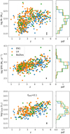 |
Fig. 1. Distributions of stellar mass (upper), SFR (middle) and AGN luminosity (bottom; only for HLIRGs with AGN fraction > 0.1) as a function of redshift for all HLIRGs. The normalized histograms are also inserted. The median uncertainty is indicated in the right bottom corner of each panel. |
2.2. Deblended Herschel 250 μm source catalogs
To explore whether HLIRGs reside in dense environments such as protoclusters with intense ongoing star formation activity, we need deep SFG catalogs. The Herschel Extragalactic Legacy Project (HELP; Shirley et al. 2019) is a large program which combines and homogenises a wide range of multi-wavelength surveys in fields observed by Herschel. HELP presents a catalog of around 170 million sources covering 1270 deg2 selected in the optical-near IR (NIR) wavelength range.
We used the deblended Herschel 250 μm source catalogs (DMU26) from HELP to search for star-forming neighbors around HLIRGs. The blind Herschel source catalogs we used to build the parent sample of IR luminous galaxies are selected by finding peaks in the matched filtered (MF) maps (Chapin et al. 2011) and thus limited to bright sources. Therefore, they are not suitable as tracers of the general SFG population. In contrast, the deblended catalogs are generated by deblending the Herschel maps based on positions of known sources in the 24 μm maps with higher resolution. They are therefore deeper than the blind Herschel source catalogs and thus better for studying the environment of HLIRGs. We use the deblended 250 μm source catalogs to search for DSFGs around HLIRGs within different projected separations and compare with those around random positions. In order to remove less reliable detections of low significance, we applied a flux density cut of 10 mJy, resulting in 42 406, 42 694, and 41 651 sources in Boötes, EN1, and LH respectively.
2.3. Deep photo-z source catalog
In order to find neighbors of HLIRGs within a certain spatial volume and characterize their environment in 3D, we need deep source catalogs that contain good-quality redshift information. SED fitting to the multi-wavelength photometry can help determine galaxy properties such as stellar mass for these sources.
We use deep source catalogs in the three deep fields compiled in Kondapally et al. (2021) to search for neighbors around our HLIRG sample. The authors generated deep source catalogs for the LH and EN1 fields and combined existing catalogs for the Boötes field. Source detection was carried out using SExtractor (Bertin & Arnouts 1996) and multi-wavelength photometry is measured first through forced, matched aperture then corrected to total fluxes using aperture corrections across all 20 and 16 bands for the EN1 and LH fields, respectively.
Photometric redshifts of the deep source catalogs were determined in Duncan et al. (2021), adopting a hybrid method that combines template fitting and machine learning. They achieve a good agreement when comparing with spectroscopic redshifts, with a 1.6–2% scatter from spectroscopic redshifts for galaxies and a 1.5–1.8% of outlier fractions (defined as |Δz|/(1 + spec − z) > 0.15).
We first applied quality flags in the three source catalogs to eliminate unreliable and duplicate sources. As explained in Kondapally et al. (2021), the FLAG_CLEAN flag indicates regions masked by bright stars and FLAG_OVERLAP flag indicates multiwavelength coverage in multiple surveys. For Boötes, an additional flag FLAG_DEEP represents duplicate sources in the I-band catalog of Brown et al. (2008). We then require the signal-to-noise ratio (S/N) in the Spitzer IRAC 3.6 μm band to be above 3σ to further reduce spurious sources, reaching a limiting magnitude of 23.63. Since our HLIRGs are all at high redshifts beyond z = 1, 3.6 μm is close to rest-frame NIR band whose emission comes mostly from evolved stellar populations. Hence, the 3.6 μm emission provides a good indicator of stellar mass (e.g., Kauffmann & Charlot 1998; Cole et al. 2001) and it suffers less dust obscuration. After applying the quality flags and S/N cuts, the total number of galaxies above z = 1 reduces to 331 032, 275 672, and 369 729 sources in the Boötes, EN1, and LH fields, respectively.
2.4. Quasar sample
Quasars are among the brightest galaxies that are powered by accretion onto their central super massive black holes (Salpeter 1964; Lynden-Bell 1969). Since the advent of large sky surveys such as the Sloan Digital Sky Survey (SDSS; York et al. 2000) and the 2dF Quasi-Stellar Object (QSO) redshift survey (2QZ; Croom et al. 2004), it has long been established that quasar clustering becomes stronger as redshift increases (Porciani et al. 2004; Croom et al. 2005; Myers et al. 2006; Shen et al. 2007). They are expected to be hosted by dark matter halos with characteristic halo masses around a few times of 1012 M⊙ with little to no dependence on quasar luminosity (Croom et al. 2005; Myers et al. 2007; Shen et al. 2007; Ross et al. 2009; White et al. 2012; Eftekharzadeh et al. 2015; Wang et al. 2015). According to the well studied relationship between stellar mass and halo mass (SMHM relationship; Guo et al. 2010; Moster et al. 2010; Behroozi et al. 2013, 2019; Wang et al. 2013; Rodríguez-Puebla et al. 2015), halos around a few times 1012 M⊙ host galaxies with stellar masses around a few times of 1010 M⊙ over a wide range of redshifts.
We used the latest SDSS sixteenth quasar catalog (Lyke et al. 2020), which consists of the largest number of spectroscopically confirmed quasars to date, with 750 414 quasars over 7500 deg2, reaching a 99.8% completeness with a contamination fraction of 0.3–1.3%. We chose to make use of this quasar catalog for several reasons. First, estimates of the host dark matter halo mass for quasar already exists thanks to extensive clustering analyses. Comparing the neighbors around HLIRGs with those around quasars can give us an indication of the environment of HLIRGs relative to the quasars. Moreover, these quasars partly overlap with our HLIRG sample in the redshift distributions as later described in Sect. 2.6. In summary, the brightness of quasars, good understanding of their host halo environment, and the overlapping redshift range allow them to make up a good sample that can serve as a cross-check.
2.5. Submillimeter galaxy sample
Submillimeter galaxies (SMGs) are rapidly star-forming galaxies at high redshifts. Their rest-frame FIR emission from obscured star-forming activity shifts towards longer wavelengths and make them detectable in the (sub)millimeter band. Overall, HLIRGs and SMGs are broadly similar in terms of their power source (i.e., dusty star formation, and AGN activity in some cases), although SMGs typically have an IR luminosity more comparable to ultraluminous IR galaxies (ULIRGs), reaching a few times of 1012 L⊙ (e.g., Chapman et al. 2005; Magnelli et al. 2012; Swinbank et al. 2014). In addition, SMGs in general are biased towards colder dust temperatures compared to Herschel-selected galaxies with similar IR luminosities (e.g., Swinbank et al. 2014; da Cunha et al. 2015).
Clustering measurements of SMGs report a strong clustering and typical host halos with Mhalo ∼ 1012 − 1013 M⊙ (Blain et al. 2004; Hickox et al. 2012; Chen et al. 2016; Wilkinson et al. 2017; Stach et al. 2021). Such halos host galaxies with stellar masses a few times of 1010 M⊙, based on the aforementioned SMHM relationship at 2 < z < 4, where the distribution of SMG peaks. Bright SMGs can be used as a signpost to trace high-redshift protocluster candidates and several studies have successfully found SMGs that reside in protoclusters (e.g., Smail et al. 2003; Daddi et al. 2009; Riechers et al. 2014; Cheng et al. 2019; Wang et al. 2021a). In our work, we also select a SMG sample to compare their neighbors with random galaxy neighbors. Similar to the quasar sample described in Sect. 2.4, by comparing HLIRG neighbors with SMG neighbors, we can find out whether HLIRGs reside in similar or more massive halos. Moreover, SMGs typically have a broadly similar redshift range (as later described in Sect. 2.6) and number distribution as HLIRGs, since they both trace dusty star-forming activity in the early universe.
The SMG sample we use is taken from Geach et al. (2017), which contains ∼3000 SMGs above 3.5σ at 850 μm over ∼5 deg2, as part of the James Clerk Maxwell Telescope (JCMT) SCUBA-2 Cosmology Legacy Survey (S2CLS). This survey reached an average 1σ depth of 1.2 mJy beam−1, close to the SCUBA-2 confusion limit of 0.8 mJy beam−1. The catalog covers six fields in total, but only the Lockman-Hole North (LH-N) field falls into the regions we study in this paper. We cross-match the 850 μm source catalog with LOFAR radio-optical cross-identified catalog in the LH field, in order to associate SMG sources with their multi-wavelength counterparts. In contrast to the quasar sample, the SMG sample suffers from small sample size and only has photometric redshifts. Therefore, when comparing both SMG neighbors and quasar neighbors with random galaxy neighbors, we can also have an idea of the influence due to small number statistics and photometric redshift uncertainty, given the fact that both samples have been well studied through clustering analyses and the quasar sample is larger and has spectroscopic redshifts. The effect from photometric redshift uncertainty is further discussed in Sect. 4.2.
2.6. Summary
Our HLIRG sample is selected from the blind Herschel catalogs. To find star-forming galaxies around HLIRGs, we took advantage of the HELP 250 μm deblended source catalogs. We also use a deep IRAC-selected source catalog with good-quality photometric redshifts in order to study the 3D environment of the HLIRGs within different spatial volumes. We also included a quasar sample (at 2 < z < 3) and a SMG sample (only in the LH field) as cross-checks.
We first restricted all samples to a limited sky area within the coverage of the deblended Herschel 250 μm source catalogs and the deep photo-z catalogs, in order to avoid searching for neighbors outside of the sky coverage. In Fig. 2, the sky areas covered by the deep photo-z catalogues are illustrated using 1000 random sources over the redshift range 2 < z < 3 for clarity. We confined all samples to be located in the central part of the regions shown by the black boxes. The sky coverage of the deblended Herschel 250 μm source catalogs is almost the same as that covered by the deep photo-z catalogs, therefore, we adopted the same limited zones. The sky area and the total number of each sample in the three fields are listed in Table 1.
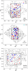 |
Fig. 2. Sky distributions of the various samples used in this study. Black dots are 1000 randomly selected sources from the deep IRAC-selected photo-z catalogs at 2 < z < 3 for clarity. We require all samples to be located inside the central black boxes in order to avoid searching for neighbors outside of the sky area coverage. HLIRGs at 2 < z < 3, redshift-matched quasars and SMGs (only in the LH field) are plotted as red circles, blue squares, and cyan squares respectively. |
Statistics of the HLIRGs, quasars, SMGs, the deblended 250 μm sources, and deep IRAC-selected photo-z catalogs in the three fields.
When exploring the star-forming neighbors of HLIRGs, we studied all HLIRGs in the limited zones and compared the number of their neighbors with the number of random galaxy neighbors. To characterize the 3D environment of HLIRG neighbors, we compared the distribution of HLIRG neighbors from the deep photo-z catalogs with the distribution of redshift-matched random galaxy neighbors. We also studied the distribution of redshift-matched quasar neighbors and SMG neighbors as cross-checks. After restriction in position according to the sky coverage of the deep photo-z catalogs, the redshift distributions of HLIRGs, quasars and SMGs are shown in Fig. 3. Our HLIRG sample lies mostly in 2 < z < 5 and quasar samples are abundant below z < 3. In spite of a small number, SMGs occupy roughly the same redshift range as HLIRGs. Based on the size of each sample, we restricted our analysis to HLIRGs at 2 < z < 4, quasars at 2 < z < 3, and SMGs at 2 < z < 4. To obtain a redshift-matched comparison, we split our HLIRG sample into 10 redshift bins with 0.2 interval over 2 < z < 4. For each redshift bin, we randomly selected the same number of quasars as the number of HLIRGs. The number of the selected SMGs is half of the number of HLIRGs, due to their small sample size. The numbers of each sample in each redshift bin are listed in Table 2.
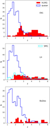 |
Fig. 3. Redshift distribution of our HLIRG (red), quasar (blue) and SMG (cyan) samples in the three deep fields after location restriction. Most HLIRGs are locacted at z > 2. SMGs have a broadly similar redshift distribution as HLIRGs, while quasars only partly overlap with the HLIRGs at 2 < z < 3. Due to small number statistics, we only study HLIRGs at 2 < z < 4 and we use quasars at 2 < z < 3 for a cross-check. |
Number of HLIRGs, redshift-matched quasars, and SMGs summed over the three fields.
3. Results
3.1. 2D surface distribution of 250 μm deblended star-formation galaxies around HLIRGs
High-redshift protoclusters are expected to be overdense regions with vigorous ongoing star formation activity. Therefore, it is reasonable to target overdensities of highly star-forming galaxies in order to identify protocluster candidates. This can be achieved by using high-resolution millimeter and submillimeter surveys to search for any overdensity of DSFGs around protocluster candidates, which can be preselected as sources with exceedingly large flux density in low-resolution surveys. For example, Planck Collaboration XXXIX (2016) presented a total of 2151 high-redshift sources whose flux density at 545 GHz are above 500 mJy and colors indicate z > 2. Optical to submillimeter observations reveal that only a small fraction are strong gravitational lensed sources and the vast majority of them (∼97%) are located in overdense regions of DSFGs. In order to further investigate the nature of these potential protoclusters, follow-up observations have been carried out. For example, SCUBA-2 observations at 850 μm (MacKenzie et al. 2017; Cheng et al. 2019, 2020) found a significant overdensity of 850 μm sources compared with blank-field distributions and a rapid ongoing star formation activity. Another example is observing unresolved bright sources detected by SPT1, a single-dish submillimeter telescope with a beam size of one arcminute (Carlstrom et al. 2011), through interferometric facilities such as ALMA (e.g, Chapman et al. 2020; Wang et al. 2021a).
We searched for deblended 250 μm sources surrounding our HLIRGs within different projected separations and compared with those of surrounding random galaxies. The ones that have more star-forming neighbors than random positions are likely to be potential protoclusters and can be used as targets for future observations to distinguish real protocluster members from chance projections. We first studied the total number of HLIRGs in the central confined region and counted the number of their neighbors within 100″. We visually inspect them and remove a few HLIRGs due to their closeness to the boundary, respectively, resulting in 27, 77, and 74 HLIRGs in Boötes, EN1, and LH respectively. We randomly select the same number of random galaxies and count their neighbors within 100″. These random galaxies are required to be located at least 200″ away from any HLIRG, to make sure that there is no overlap between HLIRG environments and random environments. We ran random selections 100 times and calculated the average distribution of the number of their neighbors. We find that HLIRGs have a median value of 13.0 ± 5.0 neighbors, while random galaxies have a median value of 11.4 ± 0.5 neighbors (calculated as the mean value and the standard deviation of median number of neighbors from 100 realizations). HLIRGs reside in an overdense environment at a 3.2σ significance level. As radius increases, the difference in environment between HLIRGs and random positions becomes weaker (with 2.9σ significance level within 200″) or may even disappear (within 400″).
To reduce contaminants from low-redshift sources, we adopted the Herschel color cut which requires S350 μm/S250 μm > 0.7 and S500 μm/S350 μm > 0.6 to effectively select sources at 1.5 < z < 3 (see Planck Collaboration XXXIX 2016). The numbers of HLIRGs occupying this redshift range are 16, 39, and 45 in Boötes, EN1 and LH, respectively; these are reduced to 16, 34, and 40 after visual inspection to remove objects near the boundary. In the upper panel of Fig. 4, we present the number distributions of star-forming neighbors around each HLIRGs within 100″ (∼1 Mpc at 1.5 < z < 3), 200″ and 400″, respectively. The black symbols and errorbars are the median values and 16th and 84th percentiles calculated from 100 realizations that select the same number of random galaxies and count their neighbors. We also require no overlap between HLIRG neighbors and random neighbors by requiring that random galaxies be locate at least two times the search radius away from every HLIRG. The cumulative distribution function (CDF) of the number of HLIRG neighbors and random neighbors are shown in the lower panel of Fig. 4. We observe a clear difference in the number of star-forming neighbors within 100″, as HLIRGs at 1.5 < z < 3 tend to have more neighbors, with a median value of 4.0 ± 2.3, compared with a median value of 2.9 ± 0.3 for random positions (calculated as the mean value and the standard deviation of median number of neighbors from 100 realizations). This difference implies that HLIRGs reside in overdense regions at a 3.7σ significance level. This difference becomes weaker as the search radius increases, reduced to 2.7 and 1.6σ for 200″ and 400″, respectively. We also adopted an IRAC color cut which requires m3.6 μm, AB − m4.5 μm, AB > −0.1 to select sources at z > 1.3 (Papovich 2008). A similar discrepancy in the number of star-forming neighbors to what has been found using the Herschel color cut also supports our expectations with regard to the overdense nature of HLIRG environments.
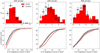 |
Fig. 4. Comparing the number of neighbors around HLIRGs to that around random positions. Upper panel: number distributions of deblended 250 μm galaxies around HLIRGs within 100, 200, and 400″, respectively. The black symbols and error bars are the median value and 16th/84th percentiles calculated from 100 realizations of random galaxies. Bottom: cumulative distribution function (CDF) of the number of HLIRG neighbors and random neighbors. HLIRGs on average have more 250 μm neighbors than random positions. This difference becomes weaker as radius increases, reducing from 3.7σ within 100″ to 2.7σ within 200″, and 1.6σ within 400″, respectively. |
3.2. Spatial distribution of IRAC-selected sources around HLIRGs
To probe the small-scale environment of HLIRGs in 3D, we searched for their neighbors using the deep IRAC-selected photo-z catalogs. In this section, we present our search for neighbors around HLIRGs and calculate the co-moving volume density of these neighbors as a function of stellar masses. We also study the neighbors around quasars and SMGs to validate our method and to explore how they compare with HLIRG neighbors.
We adopted three fixed radii: 3 Mpc, 6 Mpc, and 10 Mpc (typical scale of protoclusters, see e.g., Cai et al. 2016) to find nearby galaxies. Following Wang et al. (2021b) and Gao et al. (2021), we used CIGALE to estimate stellar mass for the deep photo-z source catalogs. We use a delayed-τ plus a starburst star formation history (SFH) and Bruzual & Charlot (2003) single stellar populations (SSPs), with a Salpeter (1955) IMF and solar metallicity. We adopted a double power-law dust attenuation law based on Charlot & Fall (2000) and dust emission models from Draine et al. (2014). We used the Fritz et al. (2006) AGN models but include fewer parameters for simplicity. We refer to Gao et al. (2021) for a detailed description of the parameter space.
Figure 5 shows the distribution of stellar mass estimates of HLIRG neighbors as well as redshift-matched quasar neighbors and random galaxy neighbors. Figure 6 shows the same distribution but only for HLIRGs in LH and redshift-matched SMGs. Dashed lines represent the stellar mass completeness limit calculated using the method described in Pozzetti et al. (2010). Briefly, we calculate the limiting stellar mass Mlimit for each galaxy which is the value a galaxy will have if its apparent 3.6 μm magnitude equals to the limiting magnitude of the entire catalog. Then, we select the 20% of the faintest galaxies in each redshift bin and assign the completeness limit as the Mlimit value below which 90% of these faint galaxies lie. The stellar masses completeness limit derived in this way is 1010.2 M⊙ and 1010.5 M⊙ in 2 < z < 3 and 3 < z < 4, respectively.
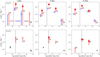 |
Fig. 5. Distribution of HLIRG neighbors (red empty circles), quasar neighbors (blue squares), and random galaxies neighbors (black stars) as a function of stellar mass. The red solid circles represent the subset of HLIRGs which are the most promising protocluster candidates (see Sect. 5). Three columns represent neighbors found within 3 Mpc, 6 Mpc, and 10 Mpc respectively. Two rows display results in two redshift bins. The dashed lines are stellar mass completeness limits in each redshift bins. We combine Poisson error, photometric redshift uncertainty, and standard deviation in the three fields for the HLIRG neighbors. We only consider sampling uncertainty for quasar neighbors and random neighbors. We find no excess in quasar neighbors at 2 < z < 3 and a weak excess in HLIRG neighbors at 3 < z < 4 compared with random neighbors. This excess disappear as searching radius increases. For the most promising protocluster candidates, we observe an enhanced excess signal. |
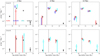 |
Fig. 6. Distribution of HLIRG neighbors (red empty circles), quasar neighbors (blue squares), SMG neighbors (cyan squares) and random galaxies neighbors (black stars) as a function of stellar mass in the LH filed. We only include Poisson error for the SMG neighbors. We also find weak excess in the SMG neighbors and this excess disappears as the search radius increases. |
In Figs. 5 and 6, the three columns represent neighbors found within different radius as indicated at the top. The two rows display two redshift bins as indicated in the upper-left corner. For the uncertainty of the HLIRGs neighbors, we combine the Poisson error, standard deviation in three fields (for Fig. 5 only) and uncertainty from photometric redshifts in quadrature. The latter comes from the standard deviation from 100 realizations. In every realization, the photometric redshift of each HLIRG is randomly determined from a Gaussian distribution, with a mean value of its photometric redshift z-photo and a standard deviation of (1+zphoto)× 0.15 (typical boundaries used for counting outliers in photometric redshift fitting, see Sect. 2.3). The data points and lower and upper boundaries for the quasar neighbors and random neighbors are median values and 16th and 84th percentiles, respectively, of 100 realizations. In each realization we randomly selected redshift-matched quasars and random positions to take uncertainty due to sampling into account. We do not consider Poisson error, standard deviation in three fields or uncertainty from photometric redshifts, because of uncertainty due to random sampling that is dominant. For the uncertainty of SMG neighbors, we only consider Poisson errors due to their small sample size.
As Figs. 5 and 6 show, there is a weak excess of HLIRG neighbors at 3 < z < 4 compared with random positions. This excess of HLIRG neighbors become weaker as the searching radius increases, implying that large-scale environment of HLIRGs is no different from random positions. The environment of quasars and SMGs within different scales is similar or marginally denser than random positions. We attribute the lack of strong excess when compared with random positions to the selection criterion of the deep photo-z catalogs we use. As explained in Sects. 2.4 and 2.5, quasars are typically hosted in dark matter halos around a few times 1012 M⊙, while SMGs are typically hosted in slightly more massive halos with masses around 1013 M⊙. Such halos will host galaxies with stellar masses a few time of 1010 M⊙. The completeness limits of our deep photo-z catalogs reach 1010.2 M⊙ and 1010.5 M⊙ in 2 < z < 3 and 3 < z < 4 respectively after applying a 3σ cut at 3.6 μm. It is expected that the environments of SMGs and quasars are similar to the environment of these massive random positions. We further discuss the influence of survey depth in Sect. 4.1. We note, additionally, that there are some studies pointing out that quasars are not good beacons of overdense structures (e.g., Trainor & Steidel 2012; Fanidakis et al. 2013; Bañados et al. 2013; Uchiyama et al. 2018).
In order to test whether the stellar mass estimates are reliable, we carried out several SED fitting runs with different models and parameters. For example, we tried different SFHs, including double power-laws and delayed-τ models without a later burst, and dust attenuation models with different slopes. We find these changes do not introduce significant systematic difference to the stellar mass estimates. We also adopted a machine learning random forest (RF) method to estimate stellar mass (described in Appendix A). When comparing HLIRG neighbors with random galaxy neighbors as a distribution of RF derived stellar mass, we find a similar picture to the one presented in Figs. 5 and 6.
3.3. Search for clusters using a FoF algorithm
In this section, we take advantage of the method used in Huang et al. (2021), whereby 88 cluster candidates were discovered, consisting of 4390 member galaxies at z < 1.1 in the 5.4 deg2 AKARI North Ecliptic Pole (NEP) field, based on photometric redshifts. The authors calculated the local density for each galaxy through the angular separation to the 10th nearest neighbour (Santos et al. 2021), then adopted a FoF algorithm to overdense galaxies in order to determine cluster members. The FoF algorithm is improved in that it considers neighbour number as a criterion for grouping friends, so that the chain-shaped linking is avoided. Also, using redshift-dependent linking length makes the FOF algorithm valid at higher redshift.
We make use of this method to find (proto)cluster candidates in deep IRAC-selected photo-z catalogs after both quality flag cuts and 3.6 μm detection significance cuts are applied (see Sect. 2.3) to reduce spurious sources which could influence the search for overdense regions. The normalized median absolute deviations (NMADs) of photometric redshift uncertainty are 0.022, 0.029, and 0.046 for Boötes, EN1, and LH fields, respectively. There are 73 974, 61 281, and 72 639 overdensities selected as having local density greater than 2 in the three fields, respectively. Then we applied the FoF algorithm on the overdensities. The projected linking length is determined by fitting the distances to the tenth neighbour for all galaxies. Having at least 10 friends within the linking length is required to continue making new friends. Clusters are selected as having more than 30 members. We find 52, 49, and 57 clusters above z > 1 in Boötes, EN1, and LH fields, respectively, with 1, 2, and 1 of them hosting HLIRGs, respectively.
The majority of our HLIRG sample are not associated with (proto)cluster candidates identified by the FoF algorithm. One explanation could be attributed to the missing overdense regions traced by the IRAC-selected photo-z catalogs. Dust-obscured overdense regions (i.e, 250 μm bright overdense regions in Sect. 3.1) may have low S/N ratios or be totally missed in the photo-z catalogs. For example, Kubo et al. (2019) found that at z ∼ 3.8, protoclusters may host obscured AGNs missed by optical selection. Therefore, the potential overdense environment which host HLIRGs cannot be identified by the FoF algorithm. Another explanation could be that HLIRGs reside in various environments and only a small fraction of them are hosted by protoclusters. We discuss this further in Sect. 4.3.
4. Discussion
4.1. Effect of survey depth
We do not find a strong excess in the quasar neighbors and SMG neighbour compared to random neighbors. The main explanation is the similar halo mass range that host quasars, SMGs, and random galaxies within our deep photo-z catalogs. In contrast, our HLIRGs are ultra-massive and, thus, they are expected to reside in dark matter halos with masses in a range of a few times of 1013 M⊙ to 1014 M⊙ at 2 < z < 3, where most of our HLIRG lie. Such extremely massive halos are expected to host a large number of member galaxies. However, we only observe a relatively weak excess in HLIRG spatial neighbors as compared to random neighbors.
We attribute this lack of excess to the fact that some HLIRG neighbors are not detected due to the limited survey depth. We selected the deep photo-z catalogs requiring 3-σ detection in the 3.6 μm band, which is sensitive to emission from evolved stars. Some star-forming neighbors of HLIRGs may be too dusty to be selected. Therefore, they are faint and of low significance in the 3.6 μm band, resulting in a non-detection in the deep photo-z catalogs. In Fig. 7, we display the normalized probabilistic distribution of 3.6 μm magnitudes for all sources in the deep photo-z catalogs, as well as neighbors of HLIRGs, quasars, and SMGs (only in the LH field). We find that HLIRG neighbors and SMG neighbors typically have fainter 3.6 μm magnitudes. It is highly possible that some neighbors are too faint in the 3.6 μm bands and are not included in our deep photo-z catalogs after applying a 3σ significance cut. We may need deeper catalogs in order to find these fainter neighbors and study the environment of HLIRGs. We anticipate that with deeper catalogs, more HLIRG neighbors will be revealed relative to the random neighbors, leading to a stronger excess signal in the HLIRG environments when making comparisons with random positions.
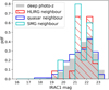 |
Fig. 7. Normalized 3.6 μm magnitudes distribution of the deep IRAC-selected photo-z catalogs (black), HLIRG neighbors (red hatched), quasar neighbors (blue) and SMG neighbors (cyan; only in the LH field) within 3 Mpc. We find that HLIRG neighbors are predominantly faint in the 3.6 μm band. |
We also explored the effect due to survey depth by seeking LOFAR-detected neighbors around HLIRGs. The sensitivity of LOFAR radio survey varies in different fields, reaching 32, 20, and 22 μJy beam−1 in Boötes, EN1, and LH fields respectively. We search for LOFAR-detected neighbors within 100″ around 64 and 198 HLIRGs in Boötes and EN1, respectively, as these two fields differ the most: after requiring a 3σ cut in the S/N of the 150 MHz detections and confining all sources to the central 14 and 24 deg2, respectively, the minimum 150 MHz flux densities are 0.16 and 0.07 mJy, respectively. We keep most of HLIRGs in the Boötes field and all HLIRGs in the EN1 field as LOFAR observations cover a large sky area. In each field, we follow the same procedure described in Sect. 3.1, searching for neighbors around HLIRGs and counting neighbors around random positions. The distribution of the number of LOFAR-detected neighbors around HLIRGs in two fields are shown in Fig. 8.
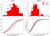 |
Fig. 8. Number distribution of LOFAR-detected neighbors around HLIRGs within 100″ compared with that around random positions in Boötes and EN1 fields, respectively. The minimum 150 MHz flux densities are 0.15 and 0.07 mJy, respectively. We find a more significant difference (4.7σ in comparison with 1.9σ) between HLIRG neighbors and random neighbors in the EN1 field, which is the deepest LOFAR field. |
As Fig. 8 shows, the difference in the abundance between HLIRG neighbors and random neighbors is larger in the EN1 field, at a 4.7σ significance level, compared to 1.9σ significance level in the Boötes field. When requiring the same depth of LOFAR detections with 150 MHz flux density > 0.5 mJy, this discrepancy in different fields disappears, reaching 1.0σ and 0.9σ significance levels, respectively. We hypothesize that deeper surveys can play an important role in studying small-scale environments, as they can include fainter and less massive galaxies which trace more typical environments with lower host halo mass values. The excess signal may become more significant when comparing HLIRG environments with these less massive environments.
4.2. The need for spectroscopic follow-ups
Another potential reason for the relatively weak excess of spatial HLIRG neighbors compared with random neighbors is due to photometric redshift uncertainty. At a given sky position, a HLIRG at 2 < z < 4 will move into a new location that is 70 − 150 Mpc away – this is beyond the scale of its host halo when its redshift is shifted with a small value of 0.1. Also, the true neighbors of HLIRGs residing in the same overdense structure could be moved outside of the searching radius due to photometric redshift uncertainty.
It is challenging to obtain spectroscopic redshifts for HLIRGs due to severe dust obscuration. So far, we have managed to obtain spectroscopic redshifts for a few HLIRGs. First, there are 28 HLIRGs (6, 8, and 14 in Boötes, EN1, and LH, respectively) that have spectroscopic redshifts that have been compiled in the deep source catalogs (Duncan et al. 2021). Second, two HLIRGs, LH_16049 and LH_23905 are observed by Northern Extended Millimeter Array (NOEMA) and their spectroscopic redshifts are consistent with photometric redshifts. LH_16049 has a zphot of 2.47 and a zspec of 2.464. LH_23905 has a zphot of 2.66 and a zspec of 2.558 (private communications with Sharon Chelsea and Axel Weiss). These two HLIRGs also demonstrate the good quality of photometric redshifts. We also obtained SUBARU observations for an extreme starburst candidate EN1_19770. The details of the observation campaign and data processing are described in the Appendix B. We retrieve a spectroscopic redshift of 3.74, which is in good agreement with the photometric redshift estimate of 3.91 in Duncan et al. (2021).
4.3. Considering whether HLIRGs are good tracers of protoclusters
We find that HLIRGs in general have more bright Herschel sources (with 250 μm flux density above 10 mJy) within 100″ than random positions at a 3.7σ significance level. However, when seeking 3D neighbors with IRAC-selected photo-z catalog, we only find relatively weak excess compared to random positions. Apart from the influence due to survey depth and photometric redshift uncertainty, another potential explanation could be attributed to HLIRG themselves. We wonder whether HLIRGs can be used as good tracers of overdense regions such as protoclusters.
From Fig. 4, we can see that around 68–87% of our HLIRGs (11 of 16, 23 of 34, and 35 of 40 in Boötes, EN1, and LH fields, respectively) have more Herschel-detected neighbors within 100″ than the median number of neighbors of random positions, while the remaining 13–32% have fewer Herschel-detected neighbors. We selected 30 HLIRGs as the most promising protocluster candidates based on the number of Herschel neighbors and FOF algorithm (see Sect. 5) and we plot the stellar mass distribution of their neighbors as red solid circles in Fig. 5. We observe a slightly enhanced excess compared to the stellar mass distribution of neighbors of all HLIRGs. We conclude that only some HLIRGs are more likely than others to reside in overdense regions, both in 2D and 3D environments. We note here that this conclusion is reached under the above-mentioned limitations of survey depth and photometric redshift uncertainty. HLIRGs that show overdensity features under such limitations can be used as the most promising candidates to identify protoclusters in follow-up observations given that spectroscopic campaigns are time-consuming (see next section). However, the possibility that HLIRGs showing no signs of overdensity in the current study may actually reside in overdense regions cannot be ruled out completely.
Miller et al. (2015) investigated a sample of mock SMGs from the Bolshoi cosmological simulation (Riebe et al. 2013; Klypin et al. 2011; Rodríguez-Puebla et al. 2016) and found that SMGs are incomplete tracers of the most-massive structures as the most majority of the most-massive structures do not host SMGs. Since the enhanced starbursting mode is short-lived, SMGs can only be observed during a relatively short period. Their rarity results in some of the most-massive structures hosting no SMGs. Moreover, due to the cosmic downsizing, the most-massive structures are expected to cease star-formation activity at an earlier epoch. Miller et al. (2015) also found that dark matter halos at z < 2.5 are less likely than their high-redshift counterparts to host SMGs. This is broadly consistent with our findings that HLIRGs at 3 < z < 4 show a relatively stronger excess than HLIRGs at 2 < z < 3, when compared with random positions.
Observationally, Chapman et al. (2015) carried out observational campaign for one of the most luminous SMGs HS1700.850.1 at z = 2.82 and concluded that it resides in relatively voids. Laporte et al. (2015) studied the environment around an extreme luminous IR galaxy HFLS3 at z = 6.34 and found no evidence for an overdensity of bright sources2. Similarly, Trainor & Steidel (2012) studied a sample of 15 most luminous QSOs at z ∼ 2.7. They found that these extremely luminous QSOs reside in host halos with masses similar to their less luminous counterparts. We cannot rule out the possibility that extreme luminous SMGs, HLIRGs, or QSOs are merely rare events and that they may not necessarily trace the most massive structures.
Overall, HLIRGs maybe a more incomplete tracers as they are rarer and more extreme than typical SMGs. This is supported by the (proto)clusters found using the FoF algorithm. Of all (proto)clusters candidates identified, > 96% of them do not host one of our HLIRGs. Nonetheless, the reason why some HLIRGs do not show an overdense nature of megaparsec-scale environment is beyond the scope of this paper. Our work aims to study the environment of the largest HLIRG sample and select the most promising protocluster candidates that would benefit further research.
5. Conclusions
In this work, we probe the megaparsec-scale environment of the largest sample of HLIRGs in three fields, in order to investigate whether they generally trace overdense regions as expected. We first searched for Herschel-detected star-forming neighbors around HLIRGs and made comparisons between them and random positions. We applied a Herschel color cut to reduce chance projections. We find that on average HLIRGs do indeed have more bright (with 250 μm flux density > 10 mJy) star-forming neighbors at a 3.7σ significance level with a median value of 4.0 ± 2.3 in their close vicinity (100″), while the median number of random neighbors is 2.9 ± 0.3.
We then searched for neighbors in 3D around HLIRGs using deep IRAC-selected photo-z catalogs. We include a quasar sample and a SMG sample as cross-checks because clustering analyses of these two samples have indicated that host dark matter halo masses are expected to be around around a few times of 1012 M⊙ and 1013 M⊙, respectively. They also (partly) overlap in redshifts with the HLIRGs. We study the comoving volume density of HLIRGs neighbors as a function of stellar mass, which we compare with that of random neighbors. We find the environment of quasars and SMGs is similar or marginally denser than the environment of random positions, mainly due to the fact that random galaxies in the IRAC-selected photo-z catalogs reside in similar massive halos based on their stellar mass estimates.
We only find relatively weak excess of HLIRG 3D neighbors compared with random neighbors. This is due to a number of factors such as the influence of survey depth, photometric redshift uncertainty which dilutes the excess signal, small number statistics, and so on. The IRAC-selected photo-z catalogs may not be able to uncover all HLIRG neighbors as they are predominantly faint at 3.6 μm. We investigate the influence due to survey depth by seeking LOFAR-detected neighbors. In the deepest EN1 field, HLIRGs have more LOFAR-detected neighbors at a 4.7σ significance level; while in the shallowest Boötes field, the excess signal is reduced to 1.9σ significance level. After applying a higher flux density cut in both fields, the significance levels drop to 1.0σ and 0.9σ, respectively, which is in agreement with our expectation. In terms of the influence of photometric redshift uncertainty, a small displacement (0.1 at 2 < z < 4) in redshift will result in a change of tens to hundreds of Mpc in location where is far away from host halos and thus no neighbors may be found. We expect that with spectroscopic redshifts, we would be able to observe a much stronger excess of massive neighbors around our HLIRGs, compared with random positions. So far, we have managed to assemble 31 spectroscopic redshifts for our HLIRG sample from literature and new optical and submillimeter observations. We also find that HLIRGs at 3 < z < 4 show stronger excess, when compared with random positions, than HLIRGs at 2 < z < 3; this is suggestive of cosmic downsizing, as the most massive halos may halt star-forming activity at 2 < z < 3 and, hence, they cannot be traced by extreme SFR.
Finally, we present a list of 30 HLIRGs in Table 3 that are ranked by the degree of overdensity in its megaparsec-scale environment. We also display the cumulative distribution of the 250 μm flux densities of their neighbors within 100″, as well as the overdensity parameters measured at different radius in Fig. C.1. We take into account factors such as the quality of their spectroscopic redshifts, the number of Herschel detected neighbors, whether or not they are associated with protocluster candidates found in the FoF algorithm and so on. Two candidates are close to the protocluster candidates identified in Greenslade et al. (2018). The authors cross-matched Herschel catalogs to Planck compact sources and selected candidates that have at least 3σ overdensities in either 250, 350, or 500 μm sources.
List of 30 HLIRGs that have been selected as the most promising signposts of potential protoclusters.
Unlike previous studies based on bright unresolved sources detected in Planck or SPT survey that have been pre-selected as protocluster candidates, our work first selects the most extreme dusty star-forming galaxies based on Herschel blind survey and we then go on to investigate their environment. We find, on average, that HLIRG have more star-forming neighbors in their close vicinity. Those having more bright neighbors are very likely to be hosted in extreme massive halos and may thus potentially reside in overdense environments, such as protoclusters. By targeting the most promising protocluster candidates with follow-up observations, we can spectroscopically confirm them and study their physical properties such as the host halo mass, total SFR, gas mass, gas depletion time, and star-formation efficiency to probe the evolution path of massive halos in an early universe.
Due to the smaller beam size of SPT (1′ compared to 3′ of Planck), SPT-detected bright sources are mostly lensed galaxies.
HFLS3 is at much higher redshift than our HLIRG sample. Both Chapman et al. (2015) and Laporte et al. (2015) searched for overdensity of LBGs which may not be a good tracer of dusty overdensities at high redshifts.
Acknowledgments
We thank Scott Trager for his help with the Subaru FOCAS spectrum analysis for the HLIRG EN1_19770. We thank Matthieu Bethermin and Giulia Rodighiero for their enlightening comments and suggestions.
References
- Arrigoni Battaia, F., Chen, C.-C., Fumagalli, M., et al. 2018, A&A, 620, A202 [NASA ADS] [CrossRef] [EDP Sciences] [Google Scholar]
- Assef, R. J., Eisenhardt, P. R. M., Stern, D., et al. 2015, ApJ, 804, 27 [Google Scholar]
- Bañados, E., Venemans, B., Walter, F., et al. 2013, ApJ, 773, 178 [CrossRef] [Google Scholar]
- Balmaverde, B., Gilli, R., Mignoli, M., et al. 2017, A&A, 606, A23 [NASA ADS] [CrossRef] [EDP Sciences] [Google Scholar]
- Behroozi, P. S., Wechsler, R. H., & Conroy, C. 2013, ApJ, 770, 57 [NASA ADS] [CrossRef] [Google Scholar]
- Behroozi, P., Wechsler, R. H., Hearin, A. P., & Conroy, C. 2019, MNRAS, 488, 3143 [NASA ADS] [CrossRef] [Google Scholar]
- Bertin, E., & Arnouts, S. 1996, A&AS, 117, 393 [NASA ADS] [CrossRef] [EDP Sciences] [Google Scholar]
- Blain, A. W., Chapman, S. C., Smail, I., & Ivison, R. 2004, ApJ, 611, 725 [NASA ADS] [CrossRef] [Google Scholar]
- Brown, M. J. I., Zheng, Z., White, M., et al. 2008, ApJ, 682, 937 [Google Scholar]
- Bruzual, G., & Charlot, S. 2003, MNRAS, 344, 1000 [NASA ADS] [CrossRef] [Google Scholar]
- Burgarella, D., Buat, V., & Iglesias-Páramo, J. 2005, MNRAS, 360, 1413 [NASA ADS] [CrossRef] [Google Scholar]
- Cai, Z., Fan, X., Peirani, S., et al. 2016, ApJ, 833, 135 [NASA ADS] [CrossRef] [Google Scholar]
- Cai, Z., Hamden, E., Matuszewski, M., et al. 2018, ApJ, 861, L3 [NASA ADS] [CrossRef] [Google Scholar]
- Calistro Rivera, G., Williams, W. L., Hardcastle, M. J., et al. 2017, MNRAS, 469, 3468 [Google Scholar]
- Capak, P. L., Riechers, D., Scoville, N. Z., et al. 2011, Nature, 470, 233 [Google Scholar]
- Cappellari, M., Emsellem, E., Krajnović, D., et al. 2011, MNRAS, 416, 1680 [Google Scholar]
- Carlstrom, J. E., Ade, P. A. R., Aird, K. A., et al. 2011, PASP, 123, 568 [CrossRef] [Google Scholar]
- Casey, C. M., Narayanan, D., & Cooray, A. 2014, Phys. Rep., 541, 45 [Google Scholar]
- Chabrier, G. 2003, PASP, 115, 763 [Google Scholar]
- Chapin, E. L., Chapman, S. C., Coppin, K. E., et al. 2011, MNRAS, 411, 505 [Google Scholar]
- Chapman, S. C., Blain, A. W., Smail, I., & Ivison, R. J. 2005, ApJ, 622, 772 [NASA ADS] [CrossRef] [Google Scholar]
- Chapman, S. C., Bertoldi, F., Smail, I., et al. 2015, MNRAS, 453, 951 [NASA ADS] [CrossRef] [Google Scholar]
- Chapman, S. C., Aravena, M. A., Ashby, M. L. N., et al. 2020, A massive protocluster at z = 7 selected by the South Pole Telescope, HST Proposal [Google Scholar]
- Charlot, S., & Fall, S. M. 2000, ApJ, 539, 718 [Google Scholar]
- Chen, C.-C., Smail, I., Ivison, R. J., et al. 2016, ApJ, 820, 82 [NASA ADS] [CrossRef] [Google Scholar]
- Cheng, T., Clements, D. L., Greenslade, J., et al. 2019, MNRAS, 490, 3840 [NASA ADS] [CrossRef] [Google Scholar]
- Cheng, T., Clements, D. L., Greenslade, J., et al. 2020, MNRAS, 494, 5985 [NASA ADS] [CrossRef] [Google Scholar]
- Chiang, Y.-K., Overzier, R., & Gebhardt, K. 2014, ApJ, 782, L3 [NASA ADS] [CrossRef] [Google Scholar]
- Cimatti, A., Cassata, P., Pozzetti, L., et al. 2008, A&A, 482, 21 [NASA ADS] [CrossRef] [EDP Sciences] [Google Scholar]
- Clements, D. L., Braglia, F. G., Hyde, A. K., et al. 2014, MNRAS, 439, 1193 [NASA ADS] [CrossRef] [Google Scholar]
- Cole, S., Norberg, P., Baugh, C. M., et al. 2001, MNRAS, 326, 255 [NASA ADS] [CrossRef] [Google Scholar]
- Cowie, L. L., Songaila, A., Hu, E. M., & Cohen, J. G. 1996, AJ, 112, 839 [Google Scholar]
- Croom, S. M., Smith, R. J., Boyle, B. J., et al. 2004, MNRAS, 349, 1397 [NASA ADS] [CrossRef] [Google Scholar]
- Croom, S. M., Boyle, B. J., Shanks, T., et al. 2005, MNRAS, 356, 415 [NASA ADS] [CrossRef] [Google Scholar]
- da Cunha, E., Walter, F., Smail, I. R., et al. 2015, ApJ, 806, 110 [Google Scholar]
- Daddi, E., Dannerbauer, H., Stern, D., et al. 2009, ApJ, 694, 1517 [Google Scholar]
- De Lucia, G., Springel, V., White, S. D. M., Croton, D., & Kauffmann, G. 2006, MNRAS, 366, 499 [NASA ADS] [CrossRef] [Google Scholar]
- Draine, B. T., Aniano, G., Krause, O., et al. 2014, ApJ, 780, 172 [Google Scholar]
- Dressler, A. 1980, ApJ, 236, 351 [Google Scholar]
- Duncan, K. J., Kondapally, R., Brown, M. J. I., et al. 2021, A&A, 648, A4 [EDP Sciences] [Google Scholar]
- Efstathiou, A., & Rowan-Robinson, M. 1995, MNRAS, 273, 649 [Google Scholar]
- Efstathiou, A., & Rowan-Robinson, M. 2003, MNRAS, 343, 322 [Google Scholar]
- Efstathiou, A., Rowan-Robinson, M., & Siebenmorgen, R. 2000, MNRAS, 313, 734 [Google Scholar]
- Efstathiou, A., Christopher, N., Verma, A., & Siebenmorgen, R. 2013, MNRAS, 436, 1873 [NASA ADS] [CrossRef] [Google Scholar]
- Eftekharzadeh, S., Myers, A. D., White, M., et al. 2015, MNRAS, 453, 2779 [Google Scholar]
- Elbaz, D., Daddi, E., Le Borgne, D., et al. 2007, A&A, 468, 33 [NASA ADS] [CrossRef] [EDP Sciences] [Google Scholar]
- Fanidakis, N., Macciò, A. V., Baugh, C. M., Lacey, C. G., & Frenk, C. S. 2013, MNRAS, 436, 315 [NASA ADS] [CrossRef] [Google Scholar]
- Farrah, D., Geach, J., Fox, M., et al. 2004, MNRAS, 349, 518 [NASA ADS] [CrossRef] [Google Scholar]
- Flores-Cacho, I., Pierini, D., Soucail, G., et al. 2016, A&A, 585, A54 [NASA ADS] [CrossRef] [EDP Sciences] [Google Scholar]
- Franck, J. R., & McGaugh, S. S. 2016, ApJ, 833, 15 [NASA ADS] [CrossRef] [Google Scholar]
- Fritz, J., Franceschini, A., & Hatziminaoglou, E. 2006, MNRAS, 366, 767 [Google Scholar]
- Gao, F., Wang, L., Efstathiou, A., et al. 2021, A&A, 654, A117 [NASA ADS] [CrossRef] [EDP Sciences] [Google Scholar]
- García-Vergara, C., Rybak, M., Hodge, J., et al. 2022, ApJ, 927, 65 [CrossRef] [Google Scholar]
- Geach, J. E., Dunlop, J. S., Halpern, M., et al. 2017, MNRAS, 465, 1789 [Google Scholar]
- Gómez, P. L., Nichol, R. C., Miller, C. J., et al. 2003, ApJ, 584, 210 [Google Scholar]
- Greenslade, J., Clements, D. L., Cheng, T., et al. 2018, MNRAS, 476, 3336 [NASA ADS] [CrossRef] [Google Scholar]
- Guo, Q., White, S., Li, C., & Boylan-Kolchin, M. 2010, MNRAS, 404, 1111 [NASA ADS] [Google Scholar]
- Hayashi, M., Kodama, T., Tadaki, K.-I., Koyama, Y., & Tanaka, I. 2012, ApJ, 757, 15 [NASA ADS] [CrossRef] [Google Scholar]
- Hickox, R. C., Wardlow, J. L., Smail, I., et al. 2012, MNRAS, 421, 284 [NASA ADS] [Google Scholar]
- Hill, R., Chapman, S., Scott, D., et al. 2020, MNRAS, 495, 3124 [NASA ADS] [CrossRef] [Google Scholar]
- Hinshaw, G., Larson, D., Komatsu, E., et al. 2013, ApJS, 208, 19 [Google Scholar]
- Huang, T.-C., Matsuhara, H., Goto, T., et al. 2021, MNRAS, 506, 6063 [NASA ADS] [CrossRef] [Google Scholar]
- Hurley, P. D., Oliver, S., Betancourt, M., et al. 2017, MNRAS, 464, 885 [Google Scholar]
- Ilbert, O., Salvato, M., Le Floc’h, E., et al. 2010, ApJ, 709, 644 [Google Scholar]
- Jones, S. F., Blain, A. W., Stern, D., et al. 2014, MNRAS, 443, 146 [Google Scholar]
- Kauffmann, G., & Charlot, S. 1998, MNRAS, 297, L23 [NASA ADS] [CrossRef] [Google Scholar]
- Kauffmann, G., White, S. D. M., Heckman, T. M., et al. 2004, MNRAS, 353, 713 [Google Scholar]
- Klypin, A. A., Trujillo-Gomez, S., & Primack, J. 2011, ApJ, 740, 102 [NASA ADS] [CrossRef] [Google Scholar]
- Kondapally, R., Best, P. N., Hardcastle, M. J., et al. 2021, A&A, 648, A3 [EDP Sciences] [Google Scholar]
- Kubo, M., Toshikawa, J., Kashikawa, N., et al. 2019, ApJ, 887, 214 [NASA ADS] [CrossRef] [Google Scholar]
- Kurk, J. D., Pentericci, L., Röttgering, H. J. A., & Miley, G. K. 2001, Ap&SS, 277, 543 [NASA ADS] [CrossRef] [Google Scholar]
- Laigle, C., McCracken, H. J., Ilbert, O., et al. 2016, ApJS, 224, 24 [Google Scholar]
- Laporte, N., Pérez-Fournon, I., Calanog, J. A., et al. 2015, ApJ, 810, 130 [NASA ADS] [CrossRef] [Google Scholar]
- Lee, K.-S., Dey, A., Hong, S., et al. 2014, ApJ, 796, 126 [Google Scholar]
- Lemaux, B. C., Le Fèvre, O., Cucciati, O., et al. 2018, A&A, 615, A77 [NASA ADS] [CrossRef] [EDP Sciences] [Google Scholar]
- Lemaux, B. C., Cucciati, O., Le Fèvre, O., et al. 2022, A&A, 662, A33 [NASA ADS] [CrossRef] [EDP Sciences] [Google Scholar]
- Lewis, I., Balogh, M., De Propris, R., et al. 2002, MNRAS, 334, 673 [NASA ADS] [CrossRef] [Google Scholar]
- Li, Q., Wang, R., Dannerbauer, H., et al. 2021, ApJ, 922, 236 [NASA ADS] [CrossRef] [Google Scholar]
- Longair, M. S., & Seldner, M. 1979, MNRAS, 189, 433 [NASA ADS] [CrossRef] [Google Scholar]
- Lyke, B. W., Higley, A. N., McLane, J. N., et al. 2020, ApJS, 250, 8 [NASA ADS] [CrossRef] [Google Scholar]
- Lynden-Bell, D. 1969, Nature, 223, 690 [NASA ADS] [CrossRef] [Google Scholar]
- MacKenzie, T. P., Scott, D., Bianconi, M., et al. 2017, MNRAS, 468, 4006 [NASA ADS] [CrossRef] [Google Scholar]
- Magnelli, B., Lutz, D., Santini, P., et al. 2012, A&A, 539, A155 [NASA ADS] [CrossRef] [EDP Sciences] [Google Scholar]
- Martinache, C., Rettura, A., Dole, H., et al. 2018, A&A, 620, A198 [NASA ADS] [CrossRef] [EDP Sciences] [Google Scholar]
- Miller, T. B., Hayward, C. C., Chapman, S. C., & Behroozi, P. S. 2015, MNRAS, 452, 878 [NASA ADS] [CrossRef] [Google Scholar]
- Miller, T. B., Chapman, S. C., Aravena, M., et al. 2018, Nature, 556, 469 [CrossRef] [Google Scholar]
- Moster, B. P., Somerville, R. S., Maulbetsch, C., et al. 2010, ApJ, 710, 903 [Google Scholar]
- Myers, A. D., Brunner, R. J., Richards, G. T., et al. 2006, ApJ, 638, 622 [NASA ADS] [CrossRef] [Google Scholar]
- Myers, A. D., Brunner, R. J., Nichol, R. C., et al. 2007, ApJ, 658, 85 [NASA ADS] [CrossRef] [Google Scholar]
- Negrello, M., González-Nuevo, J., Magliocchetti, M., et al. 2005, MNRAS, 358, 869 [CrossRef] [Google Scholar]
- Noll, S., Burgarella, D., Giovannoli, E., et al. 2009, A&A, 507, 1793 [NASA ADS] [CrossRef] [EDP Sciences] [Google Scholar]
- Nowotka, M., Chen, C.-C., Battaia, F. A., et al. 2022, A&A, 658, A77 [NASA ADS] [CrossRef] [EDP Sciences] [Google Scholar]
- Overzier, R. A. 2016, A&ARv, 24, 14 [Google Scholar]
- Papovich, C. 2008, ApJ, 676, 206 [NASA ADS] [CrossRef] [Google Scholar]
- Peng, Y.-J., Lilly, S. J., Kovač, K., et al. 2010, ApJ, 721, 193 [Google Scholar]
- Pentericci, L., Kurk, J. D., Röttgering, H. J. A., et al. 2000, A&A, 361, L25 [NASA ADS] [Google Scholar]
- Pérez-González, P. G., Rieke, G. H., Villar, V., et al. 2008, ApJ, 675, 234 [Google Scholar]
- Planck Collaboration XXXIX. 2016, A&A, 596, A100 [NASA ADS] [CrossRef] [EDP Sciences] [Google Scholar]
- Porciani, C., Magliocchetti, M., & Norberg, P. 2004, MNRAS, 355, 1010 [NASA ADS] [CrossRef] [Google Scholar]
- Pozzetti, L., Bolzonella, M., Zucca, E., et al. 2010, A&A, 523, A13 [NASA ADS] [CrossRef] [EDP Sciences] [Google Scholar]
- Riebe, K., Partl, A. M., Enke, H., et al. 2013, Astron. Nachr., 334, 691 [NASA ADS] [CrossRef] [Google Scholar]
- Riechers, D. A., Carilli, C. L., Capak, P. L., et al. 2014, ApJ, 796, 84 [Google Scholar]
- Rodríguez-Puebla, A., Avila-Reese, V., Yang, X., et al. 2015, ApJ, 799, 130 [Google Scholar]
- Rodríguez-Puebla, A., Behroozi, P., Primack, J., et al. 2016, MNRAS, 462, 893 [CrossRef] [Google Scholar]
- Ross, N. P., Shen, Y., Strauss, M. A., et al. 2009, ApJ, 697, 1634 [NASA ADS] [CrossRef] [Google Scholar]
- Rotermund, K. M., Chapman, S. C., Phadke, K. A., et al. 2021, MNRAS, 502, 1797 [NASA ADS] [CrossRef] [Google Scholar]
- Rowan-Robinson, M. 2000, MNRAS, 316, 885 [Google Scholar]
- Sabater, J., Best, P. N., Tasse, C., et al. 2021, A&A, 648, A2 [EDP Sciences] [Google Scholar]
- Salpeter, E. E. 1955, ApJ, 121, 161 [Google Scholar]
- Salpeter, E. E. 1964, ApJ, 140, 796 [NASA ADS] [CrossRef] [Google Scholar]
- Santos, D. J. D., Goto, T., Kim, S. J., et al. 2021, MNRAS, 507, 3070 [NASA ADS] [CrossRef] [Google Scholar]
- Scoville, N., Arnouts, S., Aussel, H., et al. 2013, ApJS, 206, 3 [Google Scholar]
- Shen, Y., Strauss, M. A., Oguri, M., et al. 2007, AJ, 133, 2222 [NASA ADS] [CrossRef] [Google Scholar]
- Shimakawa, R., Kodama, T., Tadaki, K. I., et al. 2014, MNRAS, 441, L1 [NASA ADS] [CrossRef] [Google Scholar]
- Shirley, R., Roehlly, Y., Hurley, P. D., et al. 2019, MNRAS, 490, 634 [Google Scholar]
- Smail, I., Ivison, R. J., Gilbank, D. G., et al. 2003, ApJ, 583, 551 [NASA ADS] [CrossRef] [Google Scholar]
- Stach, S. M., Smail, I., Amvrosiadis, A., et al. 2021, MNRAS, 504, 172 [NASA ADS] [CrossRef] [Google Scholar]
- Stalevski, M., Fritz, J., Baes, M., Nakos, T., & Popović, L. Č. 2012, MNRAS, 420, 2756 [Google Scholar]
- Steidel, C. C., Adelberger, K. L., Shapley, A. E., et al. 2005, ApJ, 626, 44 [NASA ADS] [CrossRef] [Google Scholar]
- Swinbank, A. M., Simpson, J. M., Smail, I., et al. 2014, MNRAS, 438, 1267 [Google Scholar]
- Tasse, C., Shimwell, T., Hardcastle, M. J., et al. 2021, A&A, 648, A1 [EDP Sciences] [Google Scholar]
- Thomas, D., Maraston, C., Bender, R., & Mendes de Oliveira, C. 2005, ApJ, 621, 673 [Google Scholar]
- Toshikawa, J., Uchiyama, H., Kashikawa, N., et al. 2018, PASJ, 70, S12 [NASA ADS] [CrossRef] [Google Scholar]
- Trainor, R. F., & Steidel, C. C. 2012, ApJ, 752, 39 [NASA ADS] [CrossRef] [Google Scholar]
- Tran, K.-V. H., Papovich, C., Saintonge, A., et al. 2010, ApJ, 719, L126 [CrossRef] [Google Scholar]
- Uchiyama, H., Toshikawa, J., Kashikawa, N., et al. 2018, PASJ, 70, S32 [NASA ADS] [CrossRef] [Google Scholar]
- Wang, G. C. P., Hill, R., Chapman, S. C., et al. 2021b, MNRAS, 508, 3754 [NASA ADS] [CrossRef] [Google Scholar]
- Wang, L., Farrah, D., Oliver, S. J., et al. 2013, MNRAS, 431, 648 [Google Scholar]
- Wang, L., Viero, M., Ross, N. P., et al. 2015, MNRAS, 449, 4476 [NASA ADS] [CrossRef] [Google Scholar]
- Wang, L., Gao, F., Duncan, K. J., et al. 2019, A&A, 631, A109 [NASA ADS] [CrossRef] [EDP Sciences] [Google Scholar]
- Wang, L., Gao, F., Best, P. N., et al. 2021a, A&A, 648, A8 [NASA ADS] [CrossRef] [EDP Sciences] [Google Scholar]
- White, M., Myers, A. D., Ross, N. P., et al. 2012, MNRAS, 424, 933 [NASA ADS] [CrossRef] [Google Scholar]
- Wilkinson, A., Almaini, O., Chen, C.-C., et al. 2017, MNRAS, 464, 1380 [NASA ADS] [CrossRef] [Google Scholar]
- York, D. G., Adelman, J., Anderson, J. E. Jr, et al. 2000, AJ, 120, 1579 [Google Scholar]
Appendix A: Estimate stellar mass using random forest
To explore if there is any dependence on the method by which stellar masses are estimated, we repeat the analysis on the distribution of stellar mass of neighbors with an alternative method to derive stellar masses for the IRAC-selected sources. We adopted the random forest (RF) method to derive stellar mass estimates in EN1 and trained a RF estimator with COSMOS2015 data (Laigle et al. 2016). We used the RandomForestRegressor included in Python package scikit-learn to fit the decision trees in the random forest, which creates a regression model that can be applied to the EN1 field data. We first selected the COSMOS2015 galaxies to have > 3 − σ detection in Spitzer IRAC1 band at 3.6 μm, which is the same criterion we use to reduce spurious sources in Section 2.2. Galaxies with stellar masses below 107.5 M⊙ are discarded as they may provide us with erroneously low values. We divided the COSMOS2015 data into three redshift-matched sub-samples: train, test, and validation, containing 180 931, 54 240, and 488 281 galaxies, respectively. We use seven overlapping bands between COSMOS2015 catalog and EN1 source catalog (u band data from Canada-France Hawaii Telescope; i, r, z, and y from SUBARU; 3.6 μm and 4.5 μm from Spitzer), together with the photometric redshift information, as the features for the regression model.
We use different combinations of values for the parameters max_depth (maximum depth of the three), max_features (number of features to be consider for the best split), and n_extimators (number of trees in the forest), inside RandomForestRegressor to select the best parameters in order to train the data. We start with a random search to narrow down the range and then we use the grid search to select the best parameters. We found that the best values for the RandomForestRegressor were max_depth = 31, max_features = log2(n_features), and n_extimators = 300. This led to an accuracy of ∼ 99.08% and average error of ∼ 0.084 dex for the stellar mass in both the test and validation samples. With the trained regression model, we estimate the stellar masses for 275,672 galaxies in the EN1 field (see Section 2.2). We compare them with our stellar mass estimates using CIGALE SED fitting code, finding a mean difference and standard deviation of 0.41 ± 0.27 dex. However, COSMOS2015 adopted the Chabrier (2003) IMF while we use the Salpeter (1955) IMF in this paper. Considering this difference, the mean difference reduces to ∼0.18 dex. We also compare the RF stellar masses of HLIRG neighbors with that of random galaxy neighbors and only find weak excess as discussed in Section 3.2. Thus, we conclude that the lack of significant excess of HLIRG neighbors. compared to random galaxy neighbors is not due to the method used to derive stellar masses.
Appendix B: Spectroscopic follow-up observation of the HLIRG EN1_19770
The follow-up observation of EN1_19770 was carried out on June 20th of 2021 on the Subaru 8m Telescope using the Faint Object Camera and Spectrograph (FOCAS) instrument in clear sky conditions under long slit mode, the B300 grism, and a 0.5" slit. Two 900 second integrations were taken along with associated acquisition and calibration observations. We reduced the FOCAS observations for EN1_19770, a galaxy near the field of view of galaxy LEDA 2514599. We followed the cookbook v1.0.3 of the instrument, where we performed the different steps from the raw images using IRAF version 2.16 and the FOCASRED package. First, we subtracted the offset of the images (i.e., bias) from the read-out process of the charge-coupled device (CCD). Second, we corrected the intrinsic performance of the CCDs by diving the images with the flat field taken before the observations. For this step, we used the flatnorm task to normalize the spectrum using an specified region of the average detector image. Then, we corrected the distortion pattern on the FOCAS data using the distcalib task. We calibrated the wavelength using the night sky lines for the object and the emission light from a ThAr lamp for the standard star (HZ44). We performed the sky-subtraction using the background task in IRAF by fitting the sky region close to the two galaxies located in the same slit (EN1_19770 and LEDA 2514599). We calibrated the flux with HZ44 to them combine the different exposures to remove the cosmic rays. Finally, we made a subsequent correction based on interstellar extinction and heliocentric velocity and we extracted the final 1D spectrum, as shown in Figure B.1. We derived a spectroscopic redshift of z = 3.74, based on the detection of Si IV and Si II absorption lines as shown in the figure. This source has a photometric redshift of 3.91 with a minimum value 3.82 in Duncan et al. (2021). Thus, the photometric redshift estimate agrees well with the derived spectroscopic redshift.
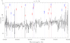 |
Fig. B.1. Optical spectrum for EN1_19770. We retrieve a spectroscopic redshift of 3.74 based on the detection of Si IV and Si II absorption lines. |
Appendix C: Overdensity of the most promising protocluster candidates
In the left panel of each subfigure in Figure C.1, we present the 250 μm flux density distribution of neighbors within 100″ of the most promising protocluster candidates. The median value and uncertainty are drawn from 100 realizations. In the right panel of each subfigure, we plot the overdensity parameter calculates as  where NHLIRG is the number of neighbors aroud HLIRGs within difference radius and Nrandom is the mean number of neighbors around random positions drawn from 100 random selections. Values above zero indicate an overdensity.
 |
Fig. C.1. Measurements for a list of 30 the most promising HLIRGs that reside in overdense regions. Left: Cumulative 250 μm flux density distribution of HLIRG neighbors within 100″ compared with random neighbors. Right: Overdensity parameters measured within different radius. |
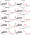 |
Fig. C.1. continued. |
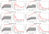 |
Fig. C.1. continued. |
All Tables
Statistics of the HLIRGs, quasars, SMGs, the deblended 250 μm sources, and deep IRAC-selected photo-z catalogs in the three fields.
Number of HLIRGs, redshift-matched quasars, and SMGs summed over the three fields.
List of 30 HLIRGs that have been selected as the most promising signposts of potential protoclusters.
All Figures
|
Fig. 1. Distributions of stellar mass (upper), SFR (middle) and AGN luminosity (bottom; only for HLIRGs with AGN fraction > 0.1) as a function of redshift for all HLIRGs. The normalized histograms are also inserted. The median uncertainty is indicated in the right bottom corner of each panel. |
| In the text | |
|
Fig. 2. Sky distributions of the various samples used in this study. Black dots are 1000 randomly selected sources from the deep IRAC-selected photo-z catalogs at 2 < z < 3 for clarity. We require all samples to be located inside the central black boxes in order to avoid searching for neighbors outside of the sky area coverage. HLIRGs at 2 < z < 3, redshift-matched quasars and SMGs (only in the LH field) are plotted as red circles, blue squares, and cyan squares respectively. |
| In the text | |
|
Fig. 3. Redshift distribution of our HLIRG (red), quasar (blue) and SMG (cyan) samples in the three deep fields after location restriction. Most HLIRGs are locacted at z > 2. SMGs have a broadly similar redshift distribution as HLIRGs, while quasars only partly overlap with the HLIRGs at 2 < z < 3. Due to small number statistics, we only study HLIRGs at 2 < z < 4 and we use quasars at 2 < z < 3 for a cross-check. |
| In the text | |
|
Fig. 4. Comparing the number of neighbors around HLIRGs to that around random positions. Upper panel: number distributions of deblended 250 μm galaxies around HLIRGs within 100, 200, and 400″, respectively. The black symbols and error bars are the median value and 16th/84th percentiles calculated from 100 realizations of random galaxies. Bottom: cumulative distribution function (CDF) of the number of HLIRG neighbors and random neighbors. HLIRGs on average have more 250 μm neighbors than random positions. This difference becomes weaker as radius increases, reducing from 3.7σ within 100″ to 2.7σ within 200″, and 1.6σ within 400″, respectively. |
| In the text | |
|
Fig. 5. Distribution of HLIRG neighbors (red empty circles), quasar neighbors (blue squares), and random galaxies neighbors (black stars) as a function of stellar mass. The red solid circles represent the subset of HLIRGs which are the most promising protocluster candidates (see Sect. 5). Three columns represent neighbors found within 3 Mpc, 6 Mpc, and 10 Mpc respectively. Two rows display results in two redshift bins. The dashed lines are stellar mass completeness limits in each redshift bins. We combine Poisson error, photometric redshift uncertainty, and standard deviation in the three fields for the HLIRG neighbors. We only consider sampling uncertainty for quasar neighbors and random neighbors. We find no excess in quasar neighbors at 2 < z < 3 and a weak excess in HLIRG neighbors at 3 < z < 4 compared with random neighbors. This excess disappear as searching radius increases. For the most promising protocluster candidates, we observe an enhanced excess signal. |
| In the text | |
|
Fig. 6. Distribution of HLIRG neighbors (red empty circles), quasar neighbors (blue squares), SMG neighbors (cyan squares) and random galaxies neighbors (black stars) as a function of stellar mass in the LH filed. We only include Poisson error for the SMG neighbors. We also find weak excess in the SMG neighbors and this excess disappears as the search radius increases. |
| In the text | |
|
Fig. 7. Normalized 3.6 μm magnitudes distribution of the deep IRAC-selected photo-z catalogs (black), HLIRG neighbors (red hatched), quasar neighbors (blue) and SMG neighbors (cyan; only in the LH field) within 3 Mpc. We find that HLIRG neighbors are predominantly faint in the 3.6 μm band. |
| In the text | |
|
Fig. 8. Number distribution of LOFAR-detected neighbors around HLIRGs within 100″ compared with that around random positions in Boötes and EN1 fields, respectively. The minimum 150 MHz flux densities are 0.15 and 0.07 mJy, respectively. We find a more significant difference (4.7σ in comparison with 1.9σ) between HLIRG neighbors and random neighbors in the EN1 field, which is the deepest LOFAR field. |
| In the text | |
|
Fig. B.1. Optical spectrum for EN1_19770. We retrieve a spectroscopic redshift of 3.74 based on the detection of Si IV and Si II absorption lines. |
| In the text | |
|
Fig. C.1. Measurements for a list of 30 the most promising HLIRGs that reside in overdense regions. Left: Cumulative 250 μm flux density distribution of HLIRG neighbors within 100″ compared with random neighbors. Right: Overdensity parameters measured within different radius. |
| In the text | |
|
Fig. C.1. continued. |
| In the text | |
|
Fig. C.1. continued. |
| In the text | |
Current usage metrics show cumulative count of Article Views (full-text article views including HTML views, PDF and ePub downloads, according to the available data) and Abstracts Views on Vision4Press platform.
Data correspond to usage on the plateform after 2015. The current usage metrics is available 48-96 hours after online publication and is updated daily on week days.
Initial download of the metrics may take a while.