| Issue |
A&A
Volume 661, May 2022
|
|
|---|---|---|
| Article Number | A149 | |
| Number of page(s) | 13 | |
| Section | The Sun and the Heliosphere | |
| DOI | https://doi.org/10.1051/0004-6361/202243234 | |
| Published online | 24 May 2022 | |
Nanoflare distributions over solar cycle 24 based on SDO/AIA differential emission measure observations
1
Institute of Physics, University of Graz, Universitätsplatz 5, 8010 Graz, Austria
e-mail: This email address is being protected from spambots. You need JavaScript enabled to view it.
2
Kanzelhöhe Observatory for Solar and Environmental Research, University of Graz, Kanzelhöhe 19, 9521 Treffen, Austria
Received:
1
February
2022
Accepted:
1
March
2022
Abstract
Aims. Nanoflares in quiet-Sun regions during solar cycle 24 are studied with the best available plasma diagnostics to derive their energy distribution and contribution to coronal heating during different levels of solar activity.
Methods. Extreme ultraviolet filters of the Atmospheric Imaging Assembly (AIA) onboard the Solar Dynamics Observatory (SDO) were used. We analyzed 30 AIA/SDO image series between 2011 and 2018, each covering a 400″ × 400″ quiet-Sun field-of-view of over two hours with a 12-s cadence. Differential emission measure (DEM) analysis was used to derive the emission measure (EM) and temperature evolution for each pixel. We detected nanoflares as EM enhancements using a threshold-based algorithm and derived their thermal energy from the DEM observations.
Results. Nanoflare energy distributions follow power laws that show slight variations in steepness (α = 2.02–2.47), but no correlation to the solar activity level. The combined nanoflare distribution of all data sets covers five orders of magnitude in event energies (1024 − 1029 erg) with a power-law index α = 2.28 ± 0.03. The derived mean energy flux of (3.7 ± 1.6)×104 erg cm−2 s−1 is one order of magnitude smaller than the coronal heating requirement. We found no correlation between the derived energy flux and solar activity. Analysis of the spatial distribution reveals clusters of high energy flux (up to 3 × 10⁵ erg cm−2 s−1) surrounded by extended regions with lower activity. Comparisons with magnetograms from the Helioseismic and Magnetic Imager demonstrate that high-activity clusters are preferentially located in the magnetic network and above regions of enhanced magnetic flux density.
Conclusions. The steep power-law slope (α > 2) suggests that the total energy in the flare energy distribution is dominated by the smallest events, that is to say nanoflares. We demonstrate that in the quiet-Sun, the nanoflare distributions and their contribution to coronal heating does not vary over the solar cycle.
Key words: Sun: activity / Sun: corona / Sun: UV radiation
© ESO 2022
1. Introduction
The temperature of the solar corona of several million Kelvin is one of the most challenging mysteries of solar physics. Ever since the discovery of the forbidden lines of highly ionized iron atoms in the coronal spectrum by Grotrian (1939) and Edlén (1943), many studies have been carried out to solve the resulting coronal heating problem. The multimillion Kelvin coronal temperature results in heat losses of at least 3 × 10⁵ erg cm−2 s−1 (Withbroe & Noyes 1977), which must be continuously balanced by energy input to prevent cooling and collapsing of the corona. However, the heat flux from the lower atmospheric layers cannot provide the required energy because the temperatures there are much lower. Consequently, some processes have to convert a nonthermal energy source into thermal energy in order to maintain the coronal plasma at stable million-Kelvin temperatures. Several models have been developed and extensively tested, and they provide us with at least part of the explanation. They can basically be assigned into two groups, which explain coronal heating either by various types of magnetized waves that are initiated by photospheric plasma motions, propagating upward into the corona and dissipating their energy there, or by small-scale magnetic reconnection events dubbed nanoflares (e.g., reviews by Klimchuk 2006; Parnell & De Moortel 2012).
Nanoflares were foreseen by Parker (1988) and could provide a solution to the coronal heating problem if they occur at a sufficiently high rate. They are the result of photospheric granular and supergranular motions that move the base of field lines in a random-walk-like manner and result in field lines that are twisted and wrapped around each other (Parker 1983). Current sheets form at the interface of misaligned flux tubes and build up free energy, which is then spontaneously released by magnetic reconnection and partially converted into thermal energy. Self-organized criticality models can explain this process of accumulation until a critical state followed by a subsequent release (Lu & Hamilton 1991). Here, regions of all sizes can be on the verge of stability and produce reconnection avalanches which are observed as flares over many orders of magnitude in event energy.
It has been shown that the occurrence frequency (dN/dE) of solar flares generally follows a power-law distribution (e.g., Dennis 1985; Crosby et al. 1993; Veronig et al. 2002; Hannah et al. 2008), which is in line with the scale invariance expected from self-organized criticality models. The power law can be expressed as a function of flare energy (E), a power-law index (α), and a normalization factor (A):
 (1)
(1)
Integration over the whole energy range (from Emin to Emax) of flares gives the total energy released:
![Mathematical equation: $$ \begin{aligned} W(E_{\min } \le E \le E_{\max }) = \int _{E_{\min }}^{E_{\max }} \frac{\mathrm{d}N}{\mathrm{d}E} E \mathrm{d}E = \frac{A}{2-\alpha } \left[E_{\max }^{-\alpha +2}-E_{\min }^{-\alpha +2}\right]. \end{aligned} $$](/articles/aa/full_html/2022/05/aa43234-22/aa43234-22-eq2.gif) (2)
(2)
Hudson (1991) first pointed out that the relative contribution of small and large flares to the total energy in such a power-law distribution critically depends on the power-law index α. In the case α > 2, the lower energy range of the frequency distribution dominates the total energy input, making it possible for nanoflares to provide sufficient energy for coronal heating. Observations of regular flares have shown that they cannot provide enough energy and that their power-law index is less than 2 (Crosby et al. 1993). In order to explain coronal heating through magnetic reconnection, the nanoflare distribution may have to become steeper than the common power law observed for large flares (Lu & Hamilton 1991). However, it has to be noted that the relative contribution alone cannot be used to determine whether the sum of all events provides enough energy.
Nanoflares are the smallest flare-like energy releases on the Sun. While regular flares and microflares occur only in active regions (e.g., Stoiser et al. 2007; Hannah et al. 2011; Fletcher et al. 2011), nanoflares also occur in quiet-Sun regions (e.g., Krucker & Benz 1998; Parnell & Jupp 2000) and they are thus a possible means to serve for the heating of the quiet (non-AR) corona. Several studies have attempted to determine the frequency distribution of nanoflares and their contribution to coronal heating. In early observational studies on nanoflares, the nanoflare energies were determined from estimates of the emission measure and temperature, which were calculated using the spectral line ratio method applied to two extreme ultraviolet (EUV) filters. Data were used either from the EUV Imaging Telescope (EIT; Delaboudinière et al. 1995) onboard the Solar and Heliospheric Observatory (SOHO) or the Transition Region and Coronal Explorer (TRACE; Handy et al. 1999). These studies on nanoflares (Krucker & Benz 1998; Parnell & Jupp 2000; Aschwanden et al. 2000; Benz & Krucker 2002; Aschwanden & Parnell 2002) enabled power laws in the range of 1.8–2.7 to be found which allowed for no definitive conclusion on whether small or large flares contribute more energy to coronal heating. The instruments used also only allow a rudimentary event energy calculation because of the limited temperature coverage of the imaged wavelengths. In a more recent study, Joulin et al. (2016) used the Atmospheric Imaging Assembly (AIA) aboard the Solar Dynamics Observatory (SDO) because of its much better plasma diagnostics and they arrive at a power-law index of 1.65 and 1.73 for the thermal event energy with background removal for an active and quiet-Sun region, respectively. They were, however, limited to precalculated DEMs from Guennou et al. (2012) which lack full AIA temporal resolution.
The listed nanoflare studies used different instruments with different spatial and temporal resolution and diagnostic capabilities. They further used different event detection methods, energies were calculated as thermal energy or radiative and conductive losses, and they also varied in other assumptions. Lastly, they focused on regions of different solar activity, ranging from quiet-Sun regions to active regions, and they were done at different times during the solar cycle. While all studies provide us with important information about nanoflare distributions in different solar regions, they are hard to compare, and we cannot conclude on how observations of similar regions might change when done at different times during the solar cycle.
By observing nanoflares in quiet-Sun regions throughout different phases of the solar cycle with the same instrument and the same detection algorithm, we can investigate as to the systematic changes to the slope of the power law, the energy input into the corona, and other nanoflare parameters and check their correlation to the level of solar activity. Any changes obtained, whether they are actual variations of the observed nanoflares or variations induced by the instrument and image properties (e.g., count rate and contrast changing due to degradation), can aid the design of future studies and help one to compare them to previous studies.
Since its launch in 2010, AIA onboard SDO has captured full disk, high spatial resolution solar images with a high cadence at multiple EUV wavelengths. The available data, therefore, cover a significant portion of solar cycle 24. Filtergrams were recorded at six coronal EUV wavelengths with different temperature responses. This allowed us to derive detailed plasma diagnostics from these images using differential emission measure (DEM) analysis.
This paper is structured as follows. In Sect. 2 we describe the data sets and DEM analysis, the developed event detection algorithm, and the event energy calculation. The results of this analysis are presented in Sect. 3. We show the observed frequency distributions, event numbers, energy flux, spatial distribution, and event areas for all data sets and correlate them to the solar activity cycle. Furthermore, the combined frequency distribution and energy flux from all data sets are derived. Section 4 follows with a discussion of the obtained power laws and their implications for the contribution to coronal heating of the detected events. Finally, in Sect. 5 we present our conclusions on the applied methods and the results obtained.
2. Methods
2.1. Data
We used data from AIA (Lemen et al. 2012) onboard SDO (Pesnell et al. 2012) which has orbited the Earth in a geosynchronous orbit since 11 February 2010. The AIA instrument consists of four individual f/20 Cassegrain telescopes with 20 cm primary optics, active secondary mirrors, and a CCD sensor with 4096 × 4096 pixels, each corresponding to a spatial sampling of the solar disk with 0.6″. With this configuration, AIA produces full disk images of the Sun in multiple wavelengths with a 1.5″ spatial resolution at a standard operating cadence of 12 s in the EUV and 24 s in the UV (Lemen et al. 2012).
We used images taken in the six EUV channels (94, 131, 171, 193, 211, and 335 Å) that are centered on wavelengths corresponding to essential iron lines at various ionization stages (Fe XVIII, Fe VIII and Fe XXI, Fe IX, Fe XII and Fe XXIV, Fe XIV, and Fe XVI). These EUV wavelength channels are not only sensitive to the line’s peak formation temperatures (log T[K]: 6.8, 5.6 and 7.0, 5.8, 6.2 and 7.3, 6.3, and 6.4), but they show a much broader temperature response that makes the chosen EUV wavelengths sensitive to plasma temperatures in a range of at least 0.1–20 MK (Lemen et al. 2012; Boerner et al. 2012).
To obtain a uniform distribution of data sets over the solar cycle, we searched for suitable image series in February, April, August, and November of each year. All image series include an observation duration of 2 h with the full AIA cadence of 12 s and focus on the center of the solar disk to minimize influences from projection effects and to have similar observation conditions for all sets. To select the data sets, beginning on the first day of the selected month, image series with the desired duration and field-of-view (FOV) were selected based on the following criteria: No active regions or coronal holes could be in the considered FOV and no flares could occur during the two-hour observation period. The exclusion of active regions and coronal holes ensured that we only included regions of the quiet-Sun in the analysis. Excluding data with simultaneous flares (even outside the considered FOV) prevents the use of short-exposure AIA images, which would result in low counts in the quiet-Sun regions and consequently poor DEM performance. If no such image series could be found for the first day of the month, the search was continued on subsequent days until all criteria were fulfilled satisfactorily. Especially at times of high solar activity, meeting all criteria was challenging, and image series of the Sun that were as quiet as possible were chosen. The availability of suitable AIA data was limited to a period from February 2011 to May 2018. The limiting factor was poor DEM reconstruction in quiet-Sun regions at the later periods, which is most probably related to the strong degradation of some of the AIA filters. A compilation of the first images of each data set is shown in Fig. 1 for the 171, 193, and 335 Å AIA filters. Line-of-sight magnetograms from the Helioseismic and Magnetic Imager (HMI; Schou et al. 2012), onboard SDO, are included for the beginning of each observation series.
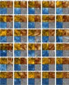 |
Fig. 1. Groups of the first AIA 171 Å, 193 Å, and 335 Å images for each of the 30 data sets plus the HMI line-of-sight magnetogram (saturated at ±15 G.) from the beginning of each observation series. All images focus on a 400″ × 400″ FOV around the center of the solar disk. The start of the observation time is displayed above each image group, and the complete data sets consist of all images taken during the two hours following the shown images. |
The selected image series were downloaded from the Joint Science Operations Center (JSOC) as full-resolution level 1 data using the available im_patch processing method, which allows images to be precropped to a tracked subimage surrounding the region of interest before downloading. We differentially rotated all acquired images of a data set to the time of the first image and then cropped them to the final dimensions of 400″ × 400″ around the center of the solar disk.
Before the DEM reconstruction, clusters of N × N pixels can be binned in the AIA maps to increase the signal-to-noise ratio. A bin factor N reduces the total number of pixels in an image by N2, increasing the DEM signal-to-noise ratio by about N, since the count rate increases by N2, while the Poisson error increases by only N. In addition, the number of pixels that deliver no DEM results or unphysical solutions (e.g., because of negative pixel values in some of the high-temperature filters) is significantly reduced. The combination of fewer unsuitable pixels and an improved signal-to-noise ratio leads, as a whole, to fewer missing solutions and more stable DEM results. A further advantage is a reduction in computation time by about N2.
However, a significant drawback is the loss of spatial resolution and consequently a possible reduction in sensitivity to events smaller than the dimensions of the binned pixel. While some binning appears necessary to obtain reliable and robust DEM results, it should be used cautiously, as detecting the smallest possible events is a critical aspect of nanoflare studies. As a compromise, we used the bin factor N = 4 for the analysis performed in this study. It strikes a good balance between reduction of the number of unusable DEM pixels on the one hand and the ability to still detect small events on the other hand. A bin factor of N = 4 results in a pixel resolution of 2.4″ for the AIA images.
As a measure of the solar activity level, we used the 13-month smoothed monthly mean sunspot number derived from the revised sunspot numbers V2.0 (Clette et al. 2014). From now on, we use the term international sunspot number (ISN) to refer to these 13-month smoothed data unless otherwise mentioned. The data were downloaded from the SILSO World Data Center (2010).
2.2. Differential emission measure analysis
We used the regularized inversion algorithm developed by Hannah & Kontar (2012) to perform the DEM analysis. Required inputs include a map structure of the six selected AIA EUV wavelength channels (94, 131, 171, 193, 211, and 335 Å), the edges of the desired temperature bins, and an AIA temperature response function. The map structures were created by using each 193 Å image in a data set as a reference and then adding the images of the other five wavelengths with the smallest time separation (typically a few seconds) from the reference image. We used a temperature range of 0.2 − 8 MK divided into 20 evenly spaced logarithmic temperature bins because we found that in this interval, the resulting solutions are well constrained by the AIA temperature sensitivity, and the range is wide enough for the quiet-Sun regions under study. To account for instrument degradation, we always applied the temperature response function for the starting time of the current data set.
Using this approach, we computed the DEM for each time step in each pixel and for all data sets. For each pixel, we then calculated the total emission measure (EM) of all temperature bins (ΔT)
 (3)
(3)
and the DEM-weighted average temperature ( ) (cf. Cheng et al. 2012; Vanninathan et al. 2015)
 (4)
(4)
for each time step.
2.3. Event detection algorithm
The detection algorithm searches for events in the derived EM time evolution of each pixel. Three user-specified parameters control crucial steps of the algorithm: the detection interval, the threshold factor, and the combination interval.
First, we compared each time step’s EM value against all previous and following values within a set interval. This detection interval is defined as the number of 12-s time steps that precede and follow the current time step. If the EM value of the current time step is higher than any other value in the interval, it is marked as a candidate event.
For each marked candidate event, the difference in the EM value relative to the minimum EM value since the last candidate event was calculated. The event was accepted if the EM change exceeded a specified threshold. This threshold was defined by multiplying a base threshold, which was calculated for each pixel individually by a global integer threshold factor. To calculate the base threshold, the standard deviation of variations in the EM evolution of each pixel from one time step to the next was used. First, the differences between successive time steps over the entire data set were calculated for each pixel. Then, the standard deviation of these differences was calculated, excluding the upper 10% of the absolute values. We did this to primarily capture EM variations caused by noise fluctuations and to exclude high values caused by actual events.
Since nanoflares can cover larger areas than a single binned AIA pixel, an algorithm had to be implemented to group detected events in neighboring pixels if they occured within a certain time interval. This interval was defined by the last parameter, the combination interval, which specifies the number of 12-s steps in each time direction in which events from adjacent pixels are combined into one event. Adjacent pixels could either include all of the surrounding eight pixels or just the ones in the x and y direction (a total of four). Previous nanoflare studies used both approaches, and there is no clear conclusion on which one should be preferred. Krucker & Benz (1998) only combined events from the nearest four neighbors with good results, and we also found this approach sufficient for combining events that cover more than one pixel. Searching a higher number of pixels for related events mainly increases random encounters and false combinations with little benefit to detecting large-scale events. Therefore, our algorithm only searches for related events in the x and y direction and omits the diagonals. We define the total area of an event as the number of pixels combined in this process.
2.4. Algorithm parameters
Poorly chosen parameters can favor or limit the detection of certain event energies and thus alter the event distribution, power-law index, and other derived nanoflare properties. However, it has already been shown that finding the perfect event definition is a very difficult task for which there is no clear solution (see Parnell 2004; Parnell & De Moortel 2012). Our experiments with different definitions and parameter settings during the development of the algorithms have shown similar variance in the final results. Thus, we do not attempt to provide a definitive answer as to the best event definition. Instead, our goal was to find reliable parameters that could be used for all data sets and provide comparable results. In addition, our event definition should be suitable for comparison with previous studies. For this aim, each parameter was tested within a reasonable range, and we then selected the most appropriate one for the final analysis.
For the event detection interval, we tested values of D = 1, 2, 3, and 4. We would like to note that D = 1 accepts only continuous, uninterrupted increases in the emission measure. During the rising phase, a single low data point splits an event into multiple segments. Furthermore, D = 2 solves this problem by allowing an event to continue after the interruption. In addition, D = 3 or 4 can provide even more visually appealing results, but they discriminate against smaller events. We have further used a detection interval of D = 2 that reduces unwanted splitting effects, but remains sensitive to the smallest events.
We tested threshold factors of F = 3, 5, 7, and 9 and found that an interval of F = 5–7 gives robust results. In particular, F = 3 results in the largest number of events found, many of which are noise, leading to numerous unwanted event combinations. With F = 5, the number of events detected decreases, as does the probability of incorrect combinations. With F = 7, the number of events decreases further, but it is still usable. At F = 9, only a small number of events remain due to the high energy threshold. In further analysis, we use F = 5 to exclude most of the noise, but count statistics still remain useful for the latter frequency analysis.
Lastly, we examined the effects of combination intervals C = 0, 1, 3, 5, 7, and 9. We found satisfactory results for values of C = 3–7. We note that C = 3 appears to be the lower acceptable limit for reliably combining larger events, while C = 5 results in even less fragmentation of large events into smaller ones and it provides more visually appealing results. Increasing this to C = 7 may be beneficial in combination with a high threshold factor (e.g., F = 7), but it generally produces results similar to C = 5. In studies using EIT data, good results have been obtained by either combining only pixels that peak simultaneously or by allowing combinations with the previous or subsequent time step. Benz & Krucker (2002) investigated the optimal time interval for combining events in studies with EIT data. They analyzed studies with intervals of ±1 to ±3 min between peaks and concluded that the optimal time interval is closer to ±1 min. Using the frequency of events found in Krucker & Benz (1998), they determined that the interval of ±3 min has a 45% chance of producing random encounters in the four adjacent pixels. This chance decreases to 15% when the interval is only ±1 min. Since our binned AIA data have a spatial resolution of 2.4″ compared to the 2.6″ of the EIT instrument, we can expect similar numbers. With an AIA image cadence of 12 s, we must use an interval of ±5 time steps to obtain the same interval of ±1 minute. This factor is what we use in the further analysis.
In summary, the selected parameter set has an event detection interval of D = 2, a threshold factor of F = 5, and an event combination interval of C = 5. For more details and illustrations of the different settings, we refer readers to the thesis of Purkhart (2021).
2.5. Event energies
We calculated the thermal energy input of the accepted EM enhancements as
 (5)
(5)
where kB is the Boltzmann constant, T is the temperature during the EM peak derived from the DEM profiles, ΔEM is the increase in emission measure in cm−5, A is the total area of the event, q is the filling factor, and h is the line-of-sight thickness of the event.
We chose a filling factor of q = 1 and estimated the line-of-sight thickness by the extent of the event as  , where A is the total event area as defined in Sect. 2.3. This definition assumes that all events are loops with a length equal to their width and has been found to give plausible results for studies comparing events over multiple energy ranges (Benz & Krucker 2002).
3. Results
3.1. Frequency distributions
Nanoflare frequency distributions were obtained by constructing a histogram from all event energies in a given data set. We divided the event energies into 50 logarithmic bins uniformly distributed over the energy range from 1023 to 1029 erg. The number of events in each group was normalized by the linear energy range covered by that bin, the two-hour observation time, and the area of the observed FOV. Figure 2 shows the created nanoflare frequency distributions for all 30 data sets. They are all characterized by a maximum event frequency at about 1024 erg (cutoff energy) with a sharp turn-over toward the lower energy range. We found that all frequency distributions closely follow a power law starting at the cutoff energy and continuing to at least 1027 erg, with some distributions extending to even higher energies up to 1029 erg.
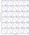 |
Fig. 2. Nanoflare frequency distribution for each data set over the years 2011–2018 during solar cycle 24. The start date and time of the corresponding data set are given on the top. Events were extracted with the detection interval set to D = 2, a threshold factor of F = 5, and a combination interval of C = 5. A linear fit (blue) without the use of the weights derived from the counting errors (red) was used to extract the power-law index (α) and its fitting error (σ). |
The measurement errors shown were derived by assuming a Poisson error statistic. Therefore, the error equals the square root of the number of events in that bin. We propagated this Poisson error through the normalization steps and the logarithmization of the histogram to obtain the displayed errors.
The power-law index α and its standard deviation σ were derived by a linear fit in log-log space starting at the energy bin with the maximum event frequency and including all nonzero frequencies of the higher energy bins. We omitted the indicated errors for the linear fit, resulting in a fit where each energy bin considered was treated with an equal weight. Therefore, a small number of large events could significantly affect the steepness of the fit and the resulting power-law index. However, we found that this method results in a linear fit that better reflects the overall slope of the frequency distributions. When Poison errors are used as weights (e.g., Joulin et al. 2016), the fit is almost entirely determined by the lower energy range since these bins contain the majority of counts. Errors from instrument noise, DEM reconstruction, threshold implementation, event combination, and energy calculation are not considered. For most of these errors, the effects on specific energy regions of the histogram are difficult to determine, but they should affect the distribution independently of the count statistics.
The individual data sets produce power-law indices in the range of 2.02–2.47 with the chosen fitting method. Figure 3 shows these derived power-law indices as a function of time and correlated to the ISN. We fit a linear function and calculated the Pearson correlation coefficient. The uncertainty range of the correlation coefficient was determined utilizing bootstrapping with 10 000 resamples. We find that the power-law index shows no significant correlation (r = 0.17 ± 0.18) to the ISN, that is to say no dependence on the solar activity level.
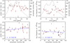 |
Fig. 3. Fitting parameters of the nanoflare frequency distributions as a function of time and correlated to the ISN. Top: power-law index α (left) and frequency at 1025 erg (right) as a function of time along with the 13-month smoothed monthly mean ISN. The fitting error for both parameters is shown as red vertical lines. Bottom: scatter plots of both fitting parameters against ISN. A linear function (blue) was fitted to the data, yielding the indicated Pearson correlation coefficient r together with the uncertainty range. |
We also show the same plots for the occurrence frequency at 1025 erg as determined by the fit. This frequency represents the second fitting parameter (A in Eq. (1)), but with the y-axis shifted to 1025 erg. This shift has the advantage that it reduces the projection of steepnesses (α) variations onto an axis that is far away and, therefore, it can be used as a better measure of the overall frequency of the observed distributions at a representative event energy. The frequency at this energy level shows a slight decrease during the years 2012 and 2013, but we found no correlation (r = −0.13 ± 0.15) to the ISN. Correlations of both parameters to the monthly mean ISN (i.e., without 13-month smoothing) were also calculated but yielded even lower coefficients of r = 0.10 ± 0.20 and r = −0.05 ± 0.15, respectively.
Since there is no dependence on the solar cycle phase, in addition to analyzing the data sets individually, we also combined them to obtain better statistics of the main nanoflare parameters in quiet-Sun regions during solar cycle 24. In Fig. 4 we present the event frequency distribution from this combined data set with a total observation time of 60 h. We used the same parameters as for the individual data sets to extract the events and fit a power law using a linear fit in log-log space without weights. The power-law fit shows good agreement with the whole frequency distribution and gives a power-law index of α = 2.28 ± 0.03. The detected events cover more than five orders of magnitude in energy and follow a close power-law distribution from 1024 to 1029 erg. The lower cutoff of the combined frequency distribution at 1024 erg is expected since all individual distributions also have their cutoff in this range with minimal variation. Individual distributions show a high energy cutoff of the continuous frequency distribution in the range of 1027–1028 erg, with only single, separated events found at even higher energies. These high energy events could have significant uncertainties since they may heavily depend on accurate event combinations between many pixels, which is one of the most challenging steps in the event detection algorithm. It is therefore promising for the developed method that the combined statistics of these large events extend the continuous part of the power-law slope up to 1028 erg, which is consistent in steepness with the lower energy part of the frequency distribution that has much better statistics.
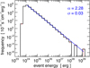 |
Fig. 4. Combined nanoflare energy distribution (black) derived from all data sets. A linear fit (blue) in log-log space without weights was used to extract the power-law index (α) and its fitting error (σ). |
Figure 5 shows the distribution of detected total event areas for the combined data sets, with the total event area being the sum of all pixels that were combined into one event. The distribution shows a clear maximum at an event size of 3.1 × 1016 cm2 (corresponding to one binned pixel, i.e., 4 × 4 original AIA pixels) and a continuous decrease in frequency for larger event sizes which follows a power law over more than three orders of magnitude to almost 1020 cm2 (corresponding to about 3000 binned pixels). For comparison, we note that this maximum area roughly corresponds to the upper range of the H-alpha subflare importance class. We fit a linear function to the distribution and derived a power-law index of α = 3.04 ± 0.09. Analysis of the individual data sets showed that they all follow a similar power-law distribution with power-law indices between 2.4 and 3.7 and no correlation (r = 0.14 ± 0.17) to the ISN.
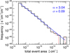 |
Fig. 5. Combined nanoflare area distribution (black) derived from all data sets. A linear fit (blue) in log-log space without weights was used to extract the power-law index (α) and its fitting error (σ). |
3.2. Energy flux and spatial distributions
The energy flux is defined as the derived thermal event energy per unit time and area and it is therefore given in units of erg cm−2 s−1. To calculate the mean energy flux of a specific data set, we first summed up the energy from all events observed in that data set and then divided the resulting total energy by the observation duration and the area of the observed FOV. This value can then be compared with the heat flux requirements needed for coronal heating in order to conclude whether the observed nanoflares provide sufficient thermal energy.
In Fig. 6 we show the observed mean energy flux for each data set and their evolution over the solar cycle and the scatter plots against the ISN. The observed mean energy flux mostly remains in the range of 2 × 10⁴ − 6 × 10⁴ erg cm−2 s−1. We found a significantly higher mean energy flux (about 1.1 × 10⁵ erg cm−2 s−1) in the data set from February 1, 2016. This results in a strong outlier that is not included in the plots. No significant correlation of the mean energy flux to the ISN was found with a correlation coefficient of r = −0.16 ± 0.14. However, a dip in the mean energy flux during the years 2012 and 2013 coincides with the decreased ISN during this period. This matches the decrease in event frequency at 1025 erg that was shown in Fig. 3 and is, therefore, likely a result of the slightly decreased overall frequency of the observed events in that time frame. From the combined energy distribution in Fig. 4, we derived a mean energy flux of (3.7 ± 1.6)×104 erg cm−2 s−1.
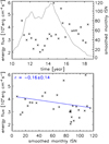 |
Fig. 6. Top: mean energy flux from nanoflares as a function of time along with the ISN. Bottom: scatter plot of mean energy flux against ISN. A linear function (blue) in log-log space was fitted to the data yielding the indicated Pearson correlation coefficient r. |
To examine the spatial distribution of the thermal energy flux in each data set, we also calculated the energy flux for each individual pixel by dividing the sum of all event energies detected in that pixel by the observation time and the area covered by just one single pixel. Figure 7 shows the obtained spatial distribution of energy flux for all data sets. We found that the energy flux is not evenly distributed across the FOV, but it forms clusters of high energy flux with extended regions of low energy flux in between.
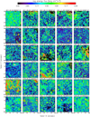 |
Fig. 7. Spatial distribution of the derived energy flux per pixel for all data sets. The beginning of each observation is annotated on top. |
In addition to smaller clusters, some data sets are also characterized by large-scale structures with high energy flux. For example, the February 1, 2016 data set, which was excluded from Fig. 6, shows extensive red bands of high energy flux (> 1.5 × 10⁵ erg cm−2 s−1) in the spatial distribution. In other regions, event observations are completely absent and therefore appear in black in the images shown. The most prominent example is found in the February 19, 2014 data set. Interestingly, most areas where no flux was detected are surrounded by areas of high energy flux. In addition, sharply outlined rectangular regions of reduced energy flux can be seen in the lower right quadrant of some of the later observations, which is most evident in the February 18, 2018 data set. The reasons for this effect remain unclear.
We plotted contours of pixels with an energy flux > 5 × 10⁴ erg cm−2 s−1 on top of HMI line-of-sight magnetograms in order to study the relationship between high energy flux regions with the underlying photospheric magnetic field. A selected image is shown in Fig. 8. We found that the areas with the highest energy flux tend to be located in the magnetic network, with a preference for boundary regions of enhanced, oppositely directed fields.
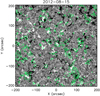 |
Fig. 8. HMI line-of-sight magnetogram with green contours marking nanoflare regions that exceed an energy flux per pixel of 5 × 10⁴ erg cm−2 s−1 over the 2-h observation time. Magnetogram is saturated at ±15 G. |
Figure 9 shows frequency distributions of the absolute magnetic flux density in pixels corresponding to different energy flux ranges. Information about the spatial distribution of the magnetic flux was extracted from the coregistered HMI line-of-sight magnetograms observed at the beginning of each data series. The figure presents the mean frequency distributions derived from the data of all data sets, excluding pixels with zero energy flux. Frequencies were derived by normalizing each bin by its absolute magnetic flux density range and the area covered by the included pixels. We found that low absolute magnetic flux densities are predominant independent of the chosen energy flux interval. However, regions with higher observed energy flux show significantly increased frequencies of regions with a higher absolute magnetic flux density. On the other hand, low energy flux regions show decreased frequencies for high absolute magnetic flux density regions compared to the overall flux density distribution. We found a mean absolute magnetic flux density of 3.1, 4.2, 5.3, 8.0, 14, and 28 G for the logarithmic energy flux intervals of < 3.83, 3.83–4.17, 4.17–4.50, 4.50–4.83, 4.83–5.17, and > 5.17 erg cm−2 s−1.
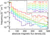 |
Fig. 9. Frequency distributions of absolute magnetic flux density in areas defined by different energy flux intervals. The whole distribution independent of the energy flux is shown as a dashed black line. |
Figure 10 shows the frequency distribution of the energy flux in all pixels from all data sets for different absolute magnetic flux density intervals of the coregistered HMI line-of-sight magnetogram. Frequencies were derived by normalizing each bin by its energy flux range and the area covered by the included pixels. We found that regions with a higher absolute magnetic flux density have increased frequencies for high energy flux regions and a reduced frequency for low energy flux regions, with a pivot point at about 3 × 10⁴ erg cm−2 s−1 for which we found about the same frequency independent of the chosen absolute magnetic flux density interval. We found a mean energy flux of 2.3, 3.3, 5.0, 5.7, 6.7, and 8.9 × 10⁴ erg cm−2 s−1 in the intervals of < 5, 5–25, 25–50, 50–100, 100–200, and > 200 G, respectively.
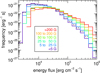 |
Fig. 10. Frequency distributions of energy flux in areas defined by different absolute magnetic flux density intervals. The whole energy flux distribution independent of the underlying magnetic flux density is shown as a dashed black line. |
In addition to the energy flux, we also examined the number of events per pixel for each data set. This allowed us to study the spatial distribution of nanoflares independent of their energy. We found that a large number of pixels (> 80%) have at least one event in all data sets, with some data sets showing activity in nearly 100% of pixels. However, the number of events is not evenly distributed, but it shows clusters of high activity that are very similar in appearance to the energy flux clusters. We also found square regions of reduced activity in the lower right corner of some data sets that match the previously discussed areas of reduced energy flux. They are characterized by a well-defined edge where the event count suddenly drops for unknown reasons. Therefore, the observed drop in energy flux is possibly due to fewer events in this area.
4. Discussion
4.1. Power law
The individual data sets from the years 2011 to 2018 produce power-law distributions that vary in steepness, with power-law indices in the range of α = 2.02–2.47. However, we found no significant correlation between the power-law index and the ISN (r = 0.17 ± 0.18). This observation is consistent with the avalanche model proposed by Lu & Hamilton (1991) and it matches the results of the frequency distributions of solar flares in hard X-rays (Crosby et al. 1993) and soft X-rays (Veronig et al. 2002).
We also did not find a correlation of the second fitting parameter (represented as the frequency at 1025 erg in Fig. 3) with the level of solar activity. These findings imply that in quiet-Sun regions, there is no change in the energy contribution by nanoflares to the coronal heating (and brightness) over the solar cycle. This is in contrast to active regions, where the contribution of regular flares changes in their occurrence frequency. As was shown in the analysis of GOES X-ray flares by Veronig et al. (2002), the overall frequency varies by more than an order of magnitude over the solar cycle, whereas, and also in this case, the shape of the distribution (α) remains constant.
We have consistently found a power-law distribution of α > 2 in all data sets, which suggests a dominance of lower energy events in the coronal heating process (Hudson 1991). This is also true for any of the other event detection parameter combinations we applied during the development of the presented method. However, they all rely on other fundamental assumptions that we did not vary. These include, in particular, the thermal energy calculation and filling factor, the scaling of the events’ line-of-sight depth relative to the detected area ( ), and the threshold calculation for the event detection.
Parnell (2004) did an extensive study where she investigated the effects of a broader range of assumptions on the observed frequency distribution. She concluded that the exact determination of frequency distributions by direct observations of nanoflares is not possible. From this investigation of 1200 differently tuned event detection and power-law extraction methods, all according to physically sensible assumptions, a wide range of frequency distributions (α = 1.5–2.6) was obtained. We note that similar considerations and caveats may apply to any nanoflare frequency studies, including the one presented here.
Figure 11 was adapted from Hannah et al. (2011) and it shows our combined nanoflare distribution together with solar nano- and microflare distributions derived by previous studies. Our distribution is very similar in steepness to the result from Benz & Krucker (2002) who found α = 2.3 ± 0.1 in their nanoflare studies using EIT data and considering the same height model as was used in this study. The spatial resolution of 2.6″ of the EIT instruments is also similar to the 2.4″ spatial resolution of the binned AIA pixels used in our study. A slightly less steep slope was found by Parnell & Jupp (2000) with a power-law index in the range of α = 2.0–2.1, using TRACE data and the same height model. Aschwanden et al. (2000) reported a smaller power-law index of α = 1.8 in their nanoflare study of TRACE data. Our results show an excellent fit to the suggested common power-law distribution of all studies, and they reach well into the microflare energy range studied by Shimizu (1995) and Hannah et al. (2008). However, we note that this comparison to microflares is somewhat deceptive as their frequency distributions are derived from soft X-ray observations with different biases and selection effects compared to the EUV nanoflares. Furthermore, microflares occur in active regions, and their occurrence rate is not independent of the solar cycle phase. We have chosen to include the microflare observations to better demonstrate the extensive energy range covered by our study and how the nanoflare energies relate to those of microflares, but we do not directly compare their power-law index and overall frequency. We refer readers to Hannah et al. (2011) for more detailed discussions on the caveats of combing the different (nano and micro) flare distributions.
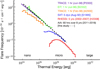 |
Fig. 11. Comparison of solar flare energy distributions derived by different studies. Shown are EUV nanoflares observed with either SOHO/EIT by Benz & Krucker (2002) or TRACE by Parnell & Jupp (2000) and Aschwanden et al. (2000). Microflares were observed with Yohkoh/SXT by Shimizu (1995) and with RHESSI by Hannah et al. (2008). The combined AIA nanoflare observations from this study is also included and indicated by the black dashed line. The figure was adapted from Hannah et al. (2011). |
What is specific about the present study is the much more extensive range of energies that is covered compared to any previous nanoflare study, spanning over five orders of magnitude. We assume that this is related to the setup of our study by (a) also being sensitive to small and short-lived events (high time cadence, multiband DEM analysis), (b) using different data sets distributed over different phases of the solar cycle, and (c) considering in the analysis in total a longer time series than previous nanoflare studies which makes it more likely to catch the less frequently occurring larger nanoflares as well. This is also seen in the frequency distributions of the individual data sets (Fig. 2), where all data sets reach to the lower energy cutoff of about 1024 erg, but not all data sets also show events > 1027 erg.
4.2. Energy flux and contribution to coronal heating
From the individual 30 data sets, we derived mean energy fluxes in the range of 2 × 10⁴–6 × 10⁴ erg cm−2 s−1 by averaging the total detected event energy of a data set over the two hour observation time and observed FOV. Our results show no significant correlation between the observed mean energy flux and the ISN. However, a slight tendency of higher energy flux in the second half of the multiyear observation period is visible, as well as a dip in energy flux in the years 2012 and 2013. For the combined distribution of all data sets, we derived a mean energy flux of (3.7 ± 1.6)×104 erg cm−2 s−1. This accounts for about 12% of the minimum heating rate of 3 × 10⁵ erg cm−2 s−1 required to heat the solar corona (Withbroe & Noyes 1977).
Krucker & Benz (1998) initially derived a thermal input of 7.1 × 10⁴ erg cm−2 s−1 in their nanoflare study, but later corrected these results with the more accurate event depth model ( ) also used in this study. They arrived at a corrected thermal energy input of about 2.2 × 10⁴ erg cm−2 s−1, which corresponds to about 7% of the minimum heating requirement. Parnell (2004) reported a thermal energy input of 2.9 × 10⁴ erg cm−2 s−1 (about 10%) for the matching height model. Thus, we found similar energy fluxes compared to these previous studies. The generally low values are an inherent problem of this type of nanoflare study and have already been discussed in detail in previous studies (e.g., Benz & Krucker 2002; Joulin et al. 2016).
Nevertheless, we can assume that the observed frequency distribution is the actual nanoflare frequency distribution and extrapolate how far the distribution would have to continue to even smaller event energies to account for 100% of the heating requirement. If we were to use the power-law index that was found for the combined data sets of α = 2.28, we would find that the distribution would have to extend down to about 5 × 10²⁰ erg, that is to say about 3.5 orders of magnitude lower than the cutoff energy in our study. This requirement moves toward higher energies if our frequency distribution underestimates either the thermal energy release per event (shift to the right) or the overall frequency (shift upward). Because of our steep slope (α > 2), an extension of the frequency distribution to larger events (above 1029 erg) only results in a negligible addition to the total energy flux.
However, calculation of the thermal energy input using the EM enhancement at the event peak (see Eq. (5)) underestimates the coronal energy input by the observed nanoflares since radiation and conduction losses already reduced the thermal energy during the event. As in nanoflares, the rise time is similar to the decay time; Benz & Krucker (2002) estimated that about half of the radiative losses occur before the event peak, which would lead to an underestimate of the thermal energy input by at least a factor of 2. Additional “unobserved” energy is needed for the expansion of chromospheric plasma, where the expansion energy exceeds the thermal energy by about a factor of 3 (Benz & Krucker 2002). The reconnection process also produces plasma motions and waves that are not observed. These considerations imply that the nanoflare energy may be up to an order of magnitude larger than the thermal energy derived at the EM peak, and they demonstrate that the above given estimate for the needed lower energy extent of the power-law distribution should only be considered a lower limit, with the actually required smallest events being at much higher energies.
4.3. Spatial distribution and magnetic characteristics of events
We analyzed the spatial distribution of events and energy flux in all data sets and found that they are not distributed homogeneously across the FOV. Instead, they form clusters with increased occurrence and extended areas of reduced activity in between.
We found that most pixels (at least 80%) are active in each data set for the used event detection parameter set. This is in contrast to Parnell & Jupp (2000), who found that only 16% (for 2σ events) of the pixels in their quiet-Sun observations contain at least one event. As the main reason, the authors give the short observation time of 15 min and note that Benz & Krucker (1999) found a significantly higher fraction of active pixels in their 42 min observations. Our high number of active pixels can presumably also be explained by the much longer observation time of 2 h per data set. Another factor could be the local threshold we set for each pixel instead of one global value. This increases the sensitivity for small events in dimmer pixels where we would otherwise not find any events.
The fraction of active pixels is also dependent on the used threshold factor. Raising the threshold factor to F = 7 brings the fraction of active pixels in all data sets down below 50% with a large portion of data sets only containing about 20% active pixels. The fraction of active pixels is further decreased to < 20% for all data sets at a threshold factor of F = 9. We conclude that the number of active pixels will approach a high fraction of the total observed pixels given a long enough observation time and a low enough threshold. However, the combined effect of both factors makes this fraction of active pixels hard to compare with different studies.
Comparisons with HMI line-of-sight magnetograms reveal that the high-activity clusters are mainly located in the magnetic network, preferentially in mixed flux regions of opposite polarities. We found that high energy flux regions show an increased frequency of absolute magnetic flux density in the coregistered HMI magnetograms compared to the overall frequency distribution. The frequency of pixels with an absolute magnetic flux density > 200 G increases by at least an order of magnitude in areas with an energy flux > 105.17 compared to the overall distribution. Furthermore, energy flux frequency distributions of different absolute magnetic flux density intervals show an increase in the frequency of high energy flux pixels in regions with a higher absolute magnetic flux density. In regions with an absolute magnetic flux density > 200 G, the occurrence frequency of pixels with an energy flux > 2 × 10⁵ erg cm−2 s−1 is increased by at least one order of magnitude compared to the overall energy flux distribution. This increase in frequency approaches nearly two orders of magnitude for pixels with an energy flux of 106 erg cm−2 s−1. At the same time, the frequency of lower magnetic flux density pixels is reduced in those same regions. The results from both the energy flux and the absolute magnetic flux density distributions show a strong correlation between our detected events and the underlying magnetic field. Together with the finding that they are preferentially located in mixed polarity regions, this makes it likely that the observed nanoflares are indeed magnetic reconnection events.
5. Conclusion
In this study, we investigated the frequency distributions of nanoflares and their characteristics in quiet-Sun regions throughout the years 2011–2018 to analyze their energy contribution to coronal heating and to study possible changes due to variations in solar activity. We used DEM analysis on the multiband EUV images from AIA, applying a threshold-based tunable event detection algorithm specifically developed for AIA data characteristics.
For all 30 data sets, we found nanoflare frequency distributions with continuous power-law slopes over multiple orders of magnitude in thermal event energy for all individual data sets. The frequency distributions calculated from the individual data sets reveal individual power-law indices in the range of α = 2.02–2.47. The parameters of the fitted power-law distributions reveal no correlation with the ISN, which indicates that the nanoflare contribution to the quiet-Sun coronal heating does not change over the solar cycle. The combined frequency distribution of all data sets, with a total observation time of 60 h at a 12-s temporal resolution, shows a power-law distribution over five orders of magnitude in thermal event energy (1024–1029 erg) with a power-law index of α = 2.28 ± 0.03, indicating that the heat input into the corona is dominated by the lower energy part of the distribution. The mean energy flux derived from the combined data set is (3.7 ± 1.6)×104 erg cm−2 s−1, which is about an order of magnitude smaller than the required coronal heat input. The observed frequency distribution would have to continue down to events with a thermal energy of about 5 × 10²⁰ erg in order to balance the total energy loss of the corona.
Regions with a large energy flux form clusters located preferentially at the boundaries of the magnetic network and show a strong correlation to the underlying absolute magnetic flux density. We found that regions with > 200 G have an increased frequency of pixels with an energy flux > 2 × 10⁵ erg cm−2 s−1 by at least one order of magnitude compared to the overall energy flux distribution. These findings suggest that the detected events are small-scale magnetic reconnection events.
Acknowledgments
AIA and HMI data are courtesy of NASA/SDO and the AIA and HMI science teams. S.P. and A.M.V. acknowledge the Austrian Science Fund (FWF): I4555-N.
References
- Aschwanden, M. J., & Parnell, C. E. 2002, ApJ, 572, 1048 [NASA ADS] [CrossRef] [Google Scholar]
- Aschwanden, M. J., Tarbell, T. D., Nightingale, R. W., et al. 2000, ApJ, 535, 1047 [Google Scholar]
- Benz, A. O., & Krucker, S. 1999, A&A, 341, 286 [NASA ADS] [Google Scholar]
- Benz, A. O., & Krucker, S. 2002, ApJ, 568, 413 [Google Scholar]
- Boerner, P., Edwards, C., Lemen, J., et al. 2012, Sol. Phys., 275, 41 [Google Scholar]
- Cheng, X., Zhang, J., Saar, S. H., & Ding, M. D. 2012, ApJ, 761, 62 [NASA ADS] [CrossRef] [Google Scholar]
- Clette, F., Svalgaard, L., Vaquero, J. M., & Cliver, E. W. 2014, Space Sci. Rev., 186, 35 [CrossRef] [Google Scholar]
- Crosby, N. B., Aschwanden, M. J., & Dennis, B. R. 1993, Sol. Phys., 143, 275 [NASA ADS] [CrossRef] [Google Scholar]
- Delaboudinière, J. P., Artzner, G. E., Brunaud, J., et al. 1995, Sol. Phys., 162, 291 [Google Scholar]
- Dennis, B. R. 1985, Sol. Phys., 100, 465 [NASA ADS] [CrossRef] [Google Scholar]
- Edlén, B. 1943, ZAp, 22, 30 [Google Scholar]
- Fletcher, L., Dennis, B. R., Hudson, H. S., et al. 2011, Space Sci. Rev., 159, 19 [Google Scholar]
- Grotrian, W. 1939, Naturwissenschaften, 27, 214 [NASA ADS] [CrossRef] [Google Scholar]
- Guennou, C., Auchère, F., Soubrié, E., et al. 2012, ApJS, 203, 26 [Google Scholar]
- Handy, B. N., Acton, L. W., Kankelborg, C. C., et al. 1999, Sol. Phys., 187, 229 [Google Scholar]
- Hannah, I. G., & Kontar, E. P. 2012, A&A, 539, A146 [NASA ADS] [CrossRef] [EDP Sciences] [Google Scholar]
- Hannah, I. G., Christe, S., Krucker, S., et al. 2008, ApJ, 677, 704 [NASA ADS] [CrossRef] [Google Scholar]
- Hannah, I. G., Hudson, H. S., Battaglia, M., et al. 2011, Space Sci. Rev., 159, 263 [NASA ADS] [CrossRef] [Google Scholar]
- Hudson, H. S. 1991, Sol. Phys., 133, 357 [Google Scholar]
- Joulin, V., Buchlin, E., Solomon, J., & Guennou, C. 2016, A&A, 591, A148 [NASA ADS] [CrossRef] [EDP Sciences] [Google Scholar]
- Klimchuk, J. A. 2006, Sol. Phys., 234, 41 [Google Scholar]
- Krucker, S., & Benz, A. O. 1998, ApJ, 501, L213 [Google Scholar]
- Lemen, J. R., Title, A. M., Akin, D. J., et al. 2012, Sol. Phys., 275, 17 [Google Scholar]
- Lu, E. T., & Hamilton, R. J. 1991, ApJ, 380, L89 [NASA ADS] [CrossRef] [Google Scholar]
- Parker, E. N. 1983, ApJ, 264, 635 [Google Scholar]
- Parker, E. N. 1988, ApJ, 330, 474 [Google Scholar]
- Parnell, C. E. 2004, in SOHO 15 Coronal Heating, eds. R. W. Walsh, J. Ireland, D. Danesy, & B. Fleck, ESA SP, 575, 227 [NASA ADS] [Google Scholar]
- Parnell, C. E., & De Moortel, I. 2012, Phil. Trans. R. Soc. London, Ser. A, 370, 3217 [Google Scholar]
- Parnell, C. E., & Jupp, P. E. 2000, ApJ, 529, 554 [Google Scholar]
- Pesnell, W. D., Thompson, B. J., & Chamberlin, P. C. 2012, Sol. Phys., 275, 3 [Google Scholar]
- Purkhart, S. 2021, Ph.D. Thesis, University of Graz, Austria [Google Scholar]
- Schou, J., Scherrer, P. H., Bush, R. I., et al. 2012, Sol. Phys., 275, 229 [Google Scholar]
- Shimizu, T. 1995, PASJ, 47, 251 [NASA ADS] [Google Scholar]
- SILSO World Data Center 2010, International Sunspot Number Monthly Bulletin and online catalogue [Google Scholar]
- Stoiser, S., Veronig, A. M., Aurass, H., & Hanslmeier, A. 2007, Sol. Phys., 246, 339 [NASA ADS] [CrossRef] [Google Scholar]
- Vanninathan, K., Veronig, A. M., Dissauer, K., et al. 2015, ApJ, 812, 173 [NASA ADS] [CrossRef] [Google Scholar]
- Veronig, A., Temmer, M., Hanslmeier, A., Otruba, W., & Messerotti, M. 2002, A&A, 382, 1070 [NASA ADS] [CrossRef] [EDP Sciences] [Google Scholar]
- Withbroe, G. L., & Noyes, R. W. 1977, ARA&A, 15, 363 [Google Scholar]
All Figures
|
Fig. 1. Groups of the first AIA 171 Å, 193 Å, and 335 Å images for each of the 30 data sets plus the HMI line-of-sight magnetogram (saturated at ±15 G.) from the beginning of each observation series. All images focus on a 400″ × 400″ FOV around the center of the solar disk. The start of the observation time is displayed above each image group, and the complete data sets consist of all images taken during the two hours following the shown images. |
| In the text | |
|
Fig. 2. Nanoflare frequency distribution for each data set over the years 2011–2018 during solar cycle 24. The start date and time of the corresponding data set are given on the top. Events were extracted with the detection interval set to D = 2, a threshold factor of F = 5, and a combination interval of C = 5. A linear fit (blue) without the use of the weights derived from the counting errors (red) was used to extract the power-law index (α) and its fitting error (σ). |
| In the text | |
|
Fig. 3. Fitting parameters of the nanoflare frequency distributions as a function of time and correlated to the ISN. Top: power-law index α (left) and frequency at 1025 erg (right) as a function of time along with the 13-month smoothed monthly mean ISN. The fitting error for both parameters is shown as red vertical lines. Bottom: scatter plots of both fitting parameters against ISN. A linear function (blue) was fitted to the data, yielding the indicated Pearson correlation coefficient r together with the uncertainty range. |
| In the text | |
|
Fig. 4. Combined nanoflare energy distribution (black) derived from all data sets. A linear fit (blue) in log-log space without weights was used to extract the power-law index (α) and its fitting error (σ). |
| In the text | |
|
Fig. 5. Combined nanoflare area distribution (black) derived from all data sets. A linear fit (blue) in log-log space without weights was used to extract the power-law index (α) and its fitting error (σ). |
| In the text | |
|
Fig. 6. Top: mean energy flux from nanoflares as a function of time along with the ISN. Bottom: scatter plot of mean energy flux against ISN. A linear function (blue) in log-log space was fitted to the data yielding the indicated Pearson correlation coefficient r. |
| In the text | |
|
Fig. 7. Spatial distribution of the derived energy flux per pixel for all data sets. The beginning of each observation is annotated on top. |
| In the text | |
|
Fig. 8. HMI line-of-sight magnetogram with green contours marking nanoflare regions that exceed an energy flux per pixel of 5 × 10⁴ erg cm−2 s−1 over the 2-h observation time. Magnetogram is saturated at ±15 G. |
| In the text | |
|
Fig. 9. Frequency distributions of absolute magnetic flux density in areas defined by different energy flux intervals. The whole distribution independent of the energy flux is shown as a dashed black line. |
| In the text | |
|
Fig. 10. Frequency distributions of energy flux in areas defined by different absolute magnetic flux density intervals. The whole energy flux distribution independent of the underlying magnetic flux density is shown as a dashed black line. |
| In the text | |
|
Fig. 11. Comparison of solar flare energy distributions derived by different studies. Shown are EUV nanoflares observed with either SOHO/EIT by Benz & Krucker (2002) or TRACE by Parnell & Jupp (2000) and Aschwanden et al. (2000). Microflares were observed with Yohkoh/SXT by Shimizu (1995) and with RHESSI by Hannah et al. (2008). The combined AIA nanoflare observations from this study is also included and indicated by the black dashed line. The figure was adapted from Hannah et al. (2011). |
| In the text | |
Current usage metrics show cumulative count of Article Views (full-text article views including HTML views, PDF and ePub downloads, according to the available data) and Abstracts Views on Vision4Press platform.
Data correspond to usage on the plateform after 2015. The current usage metrics is available 48-96 hours after online publication and is updated daily on week days.
Initial download of the metrics may take a while.