| Issue |
A&A
Volume 684, April 2024
|
|
|---|---|---|
| Article Number | A60 | |
| Number of page(s) | 10 | |
| Section | The Sun and the Heliosphere | |
| DOI | https://doi.org/10.1051/0004-6361/202348199 | |
| Published online | 04 April 2024 | |
Solar nanoflares in different spectral ranges
1
Samara National Research University, Samara 443086, Russia
2
Lebedev Physical Institute, Russian Academy of Sciences, Moscow 119991, Russia
e-mail: This email address is being protected from spambots. You need JavaScript enabled to view it.
3
Space Research Institute, Moscow 117997, Russia
4
Sternberg Astronomical Institute, Lomonosov Moscow State University, Moscow 119234, Russia
Received:
8
October 2023
Accepted:
23
January 2024
Abstract
Aims. The rates and other characteristics of solar nanoflares were measured for the same area of the Sun in different extreme-ultravioilet (EUV) channels to find how the main properties of nanoflares depend on the spectral range.
Methods. We used images of the quiet Sun obtained by the Atmospheric Imaging Assembly (AIA) on board the Solar Dynamics Observatory (SDO) in seven spectral channels, 94 Å, 131 Å, 171 Å, 193 Å, 211 Å, 304 Å, and 335 Å. We analyzed 300 images for each AIA/SDO channel covering one hour from 12:00 UT to 13:00 UT on 20 May 2019 with a 12 s cadence. We searched for nanoflares in two 360″×720″ fields of view above (N) and below (S) the Sun’s equator to measure nanoflare latitudinal distributions and their N–S asymmetry. To detect nanoflares, we used a threshold-based algorithm with 5σ threshold.
Results. The integral nanoflare rate measured in seven spectral ranges is 3.53 × 10⁻²¹ cm−1 s−1; the corresponding frequency is 215 events s−1 for the entire surface of the Sun. A search for nanoflares in any single AIA-channel leads to significant underestimation of their frequency and rate: 171 Å −34% of the total value; 193 Å −33%; 211 Å −24%; other channels – less than 16%. Most EUV nanoflares are single-pixel (∼78%) and mono-channel (∼86%) events. In channel 304 Å, multipixel events dominate over single-pixel events (68% vs. 32%). The average duration of nanoflares is in the range of (89 − 141)±(40 − 61) s depending on the spectral region with the mean value being 129 ± 59 s. The latitudinal distribution of nanoflares is approximately uniform in the range from 0° to 45° for all channels. We find a slight difference between the N and S hemispheres (up to 20% depending on channel), but we do not find it to be statistically significant.
Conclusions. We demonstrate that solar nanoflares can be found in all AIA EUV channels. The detection probability strongly depends on the spectral range and the channels can be approximately ranked as follows (from high to low probability): 171 Å, 193 Å, 211 Å, 131 Å, 304 Å, 335 Å, and 94 Å. The first three channels, 171, 193, and 211 Å, allow the detection of ∼78% of all the nanoflares. The remaining four add only 22%. Other characteristics of nanoflares, including duration and spatial distribution, weakly depend on spectral range.
Key words: Sun: corona / Sun: flares / Sun: UV radiation
© The Authors 2024
 Open Access article, published by EDP Sciences, under the terms of the Creative Commons Attribution License (https://creativecommons.org/licenses/by/4.0), which permits unrestricted use, distribution, and reproduction in any medium, provided the original work is properly cited.
This article is published in open access under the Subscribe to Open model. This email address is being protected from spambots. You need JavaScript enabled to view it. to support open access publication.
1. Introduction
Solar nanoflares are small-scale energy-release events located in the low layers of the solar atmosphere (Hudson 1991; Bogachev et al. 2020). The term “nanoflares” was originally coined by Parker (1988) in relation to energy content: nanoflares are smaller than microflares with energies ranging 1024 − 1027 erg per event. For decades, these events were considered as one of the possible mechanisms to explain the heating of the solar corona to the observed high temperatures (Parker 1983; Erdélyi & Ballai 2007; Priest et al. 2018; Aschwanden 2022). Analysis of solar radiation in the extreme ultraviolet (EUV) spectral range (∼10 − 100 nm) revealed that nanoflares can be easily found almost everywhere in the quiet corona. Usually, these events are observed as a short-term brightening that lasts from several tens of seconds to several minutes and covers one or a few pixels in solar EUV images (corresponding to a linear size of several hundred to several thousand km). Given this description, nanoflares are very similar to smaller copies of ordinary solar flares (Ulyanov et al. 2019a), which explains the term “flare” in their name. However, this does not mean that the physics related to nanoflares is the same as that of ordinary flares. The question of whether or not nanoflares are simply small-scale flares or are a distinct class of events still has no definitive answer.
In general, there are a variety of small-scale processes in the solar atmosphere, and not all of them can be classified as nanoflares. For this reason, the term brightening is often used for the description of this type of solar activity, in an effort to emphasize that we only detect small-scale brightness increases, but do not specify their nature. Contrary to this approach, in our study, we use the term nanoflare. This means that we consider only small-scale impulsive coronal events seen in EUV spectral ranges with a temperature of about 1 MK and with a duration of no more than a few minutes. We believe that these criteria define the ensemble of nanoflares quite well and at least allow us to isolate them from similar chromospheric phenomena, such as Ellerman bombs (Ortiz et al. 2020), and from X-ray bright points (Mondal et al. 2023), which usually have larger sizes and longer lifetimes.
Due to the small scale and low brightness of the nanoflare events, their detection requires not only high sensitivity of the instrument but also a reasonable selection of the spectral range for observations. Most studies of nanoflares to date were carried out in the 171 Å and 193/195 Å spectral ranges using the TRACE, SoHO/EIT, and SDO/AIA instruments (Parnell & Jupp 2000; Aschwanden et al. 2000; Aschwanden & Parnell 2002; Krucker & Benz 1998; Benz & Krucker 2002; Ulyanov et al. 2019b). Both channels (171 Å and 193/195 Å) have a maximum temperature sensitivity of near T ∼ 1 MK, which approximately corresponds to the temperature of the quiet solar corona. The fact that the temperature of nanoflares is close to the temperature of the surrounding plasma suggests that their increase in brightness is more associated with an increase in the emission measure than with an increase in temperature, although both effects clearly contribute.
It should be noted that in most studies of nanoflares, analyses are limited to the consideration of one or two channels. For this reason, we would like to draw attention to recent works by Purkhart & Veronig (2022) and Joulin et al. (2016). Here, the authors carried out multiwavelength studies of nanoflares based on measurements of their differential emission measure (DEM; for a comparison of the results from different DEM reconstruction algorithms see e.g., Massa et al. 2023). A brief comparison of the experimental results obtained using single-channel and multichannel techniques is given in Table 1. The event frequency shown in Table 1 is given in terms of the total surface of the Sun. For those articles where the frequency was not given by the authors (we mark the event frequency with an asterisk), we estimated it from the number of observed events, the area of the solar surface under study, and the observation time. The large spread in event frequency is due to many factors: different instrument sensitivities, different nanoflare detection thresholds, different physical conditions on the Sun, and so on.
Nanoflare observations.
Regarding multichannel nanoflare analyses, one cannot help but notice that the ability to study solar nanoflares has increased significantly thanks to SDO/AIA telescopes (Lemen et al. 2011) launched in 2010, which provide approximately simultaneous images of the Sun in seven EUV spectral ranges, six of which are related to the solar corona (94 Å, 131 Å, 171 Å, 193 Å, 211 Å, and 335 Å) and one is related to the transition region (304 Å). In the literature, the 304 Å channel is generally presented as a chromospheric channel, although it mainly registers the emission of He II with a characteristic temperature ∼5 × 10⁴ K. This emission is formed in the transition region between the chromosphere and the corona. For this reason, we associate channel 304 Å with the transition region. In addition to multiwavelength analyses (e.g., DEM reconstruction), the amount of available data also allows us to compare different spectral ranges and therefore to answer the question of which channel or group of channels is the most favorable for the detection and study of solar nanoflares. More generally, we would like to know how the main characteristics of solar nanoflares (frequency, duration, etc.) differ when observed in different spectral ranges. To answer the stated questions, we performed an independent search for solar nanoflares in the seven SDO/AIA channels listed above using the same method for all these spectral ranges. In doing so, we paid special attention to channels 94 Å and 335 Å, which correspond to higher plasma temperatures than the others (see Table 2 with the list of SDO/AIA channels and corresponding temperatures). These two channels are usually excluded from consideration because of the low signal-to-noise ratio, and we were interested in finding a way to obtain valid information for them. We also wanted to estimate the probability of finding a high-temperature component in nanoflares. We included the 304 Å channel (another spectral range that is rarely used in studies of nanoflares) to understand how many coronal nanoflares produce a pronounced response in the underlying solar transition region, where the main emission in the He II 304 Å line is formed.
Brief overview of the used AIA channels.
In addition, to increase the number of events, and consequently to increase the statistical validity of the results obtained, we separately studied nanoflares in the northern and southern hemispheres of the Sun. Through this approach, we were also able to test whether or not there is an asymmetry between the rate of nanoflares in the different hemispheres of the Sun.
Our paper is organized as follows. First, in Sect. 2, we discuss the data we used together with the methods used to process them. We also describe the algorithms used to search for nanoflares. Next, in Sect. 3, we outline the obtained results, and finally, in Sect. 4, we draw conclusions.
2. Data and methods
Our study is based on data obtained by the Atmospheric Imaging Assembly (AIA) instrument operating on board the Solar Dynamics Observatory (SDO). The AIA is a four-telescope array with sensitivity in extreme ultraviolet (EUV), UV, and visible spectral ranges. This instrument provides full-disk images of the Sun with a size of 4096 × 4096 pixels, a resolution of 0.6″ per pixel, and a cadence of 12 s. A significant advantage of AIA, which is especially important for our study, is the large number of spectral ranges it offers; that is, ten channels. For our purposes, we take into consideration only seven of these, namely those related to the EUV range. The list of these channels and their main characteristics are given in Table 2.
Among the listed EUV channels, the majority, six out of seven, belong to the solar corona. Channel 304 Å belongs to the transition region of the Sun, and therefore the brightenings visible in this channel cannot be directly attributed to nanoflare events. On the other hand, it is well known that ordinary solar flares, being coronal phenomena, also generate intense radiation from the chromosphere and the transition region of the Sun. We therefore included the 304 Å channel in our data set; not to study nanoflares, but as a source of information about the response of the solar transition region to impacts from nanoflares. Channels 131 Å and 193 Å as shown in Table 2 have high sensitivity not only in the temperature range ∼106 K, where the main radiation of nanoflares is formed, but also in the temperature range ∼107 K. However, we do not believe that plasma with such a high temperature can be formed in solar nanoflares, and we consider both of these channels to be related to the quiet corona within the framework of the present study. Channel 94 Å is believed to only produce a noticeable signal in solar flares and for this reason has a very low intensity in the quiet solar corona. We estimated the average signal in the channel to be 0.38 counts pix−1 s−1 in the quiet corona and 2.3 counts pix−1 s−1 in nanoflares. Another channel with a very low signal-to-noise ratio is 335 Å (0.32 counts pix−1 s−1 in the quiet corona and 2.34 counts pix−1 s−1 in nanoflares). In our study, we tried to take into account the mentioned features of the channels under consideration.
We used AIA data obtained on 20 May 2019 from 12:00 UT to 13:00 UT (duration – 1 h) during a period of low solar activity (solar minimum between cycles 24 and 25). At this time, there were no sunspots, active regions, or solar flares on the visible side of the Sun. From all other points of view, the time period was chosen arbitrarily and had no other features. As the AIA cadence is 12 s, the number of images in each channel is 300 (total number of images – 2100). The search for nanoflares was carried out in two rectangular frames, each with a size of 600 × 1200 pixels, which were located symmetrically relative to the solar equator in the northern and southern hemispheres (see Fig. 1). Angle B0 (heliographic latitude of the central point of the solar disk) on 20 May 2019 was only 2.15°. Taking this into account, we further neglect the difference between the apparent and real position of the solar equator and believe that the difference between them is insignificant. Each fragment covers a region that lies approximately in the range [0°, 49.4°] for the northern hemisphere and [0°, −49.4°] for the southern hemisphere along solar latitude and in the range of about ±11° (at the equator) along solar longitude.
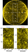 |
Fig. 1. Sun in the SDO/AIA 171 Å channel for 20 May 2019 11:59:59 UT. White rectangles denote the areas where nanoflares were searched. |
The surface area of each fragment is equal to
 (1)
(1)
where S⊙ is the total surface area of the Sun.
The procedure for searching for nanoflares was typical for this type of research and is based on the idea of searching for brightenings with an amplitude that exceeds the average “background” in a given pixel by more than 5σ, where σ is the standard deviation of the signal in this pixel during the observation time. Modifications of this method used by different authors differ from each other in the presence or absence of binning; in the method of background subtraction; in the threshold value for separating nanoflares from noise; and in the method of combining neighboring brightenings into one event. We did not use binning, and examined the original AIA images with a maximum spatial resolution of 0.6″ per pixel. Regarding the threshold value, for a data cube of 600 × 1200 × 300, the 5σ level gives
for one channel. For a 3σ threshold, the number of random events (noise events misinterpreted as nanoflares) would be ∼3 × 10⁵. Our estimation of the energy range of the nanoflares corresponding to the 5σ criterion used can be found in Sect. 4.
Let us now outline the methods of background subtraction and pixel clustering. In general, our procedure for AIA data processing and searching for nanoflares consists of the following steps:
-
First, all images were processed to AIA 1.5 level using the aiapy Python package (Barnes et al. 2020a). During this step, the differential rotation was compensated using the propagate_with_solar_surface method of the SunPy package (Barnes et al. 2020b)
-
All data were then transformed into data cubes I(x, y, n), where n = 1…300 is the image number, and x, y are pixel coordinates: x = 1…600, y = 1…1200.
-
Although the AIA images of level 1.5 are cleared of spike events (bright tracks from charged particles), we applied additional cleaning as we were still detecting the impact of this effect. For this purpose, we excluded from consideration all the pixels where the signal increased by more than 3σ in one step and then decreased by more than 3σ in the subsequent step. This simple filter effectively removes even extremely faint spikes and gives only one false registration per 600 × 1200 frame. The filter will also remove hypothetical nanoflares with a "lifetime" of less than 12 s (AIA cadence), but we believe that such a short lifetime is not typical for nanoflares exceeding the threshold 5σ.
-
The nanoflare search is based on the examination of the time profiles measured in each individual pixel: Ixy(t)=I(x, y, n = 1…300). An example of such a time profile is shown in Fig. 2. The signal in each pixel usually consists of a slowly changing substrate (background) and a rapidly changing component, the main cause of which is photon noise. To extract the slowly changing background, we used the median filter with a kernel of 25 points (300 s). The kernel size was chosen so as not to be sensitive to signal variations with a characteristic time of ∼100 s, which we consider as candidates for nanoflares. The time profile after background subtraction is shown in the bottom panel of Fig. 2. For this cleaned profile, we determined the standard deviation σ and then defined nanoflares as brightenings with an amplitude of greater than the 5σ threshold. At the beginning and the end of the nanoflare, we considered the two closest points located to the left and to the right of the maximum, which are lower than the 2 (±2) neighboring points.
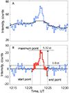 |
Fig. 2. Method used to search for nanoflares in the present study. A real nanoflare in channel 171 Å is used as an example. |
For clarity, we explain this approach in greater detail in the bottom panel of Fig. 2. Using this method, we found 157 712 one-pixel nanoflares, which were distributed between the AIA channels as shown in Table 3.
Another important step in identifying different events is clustering. A nanoflare can cover more than 1 pixel, which raises the question of how to combine single-pixel brightenings into one multipixel event. Clustering techniques vary from one study to another (see e.g., Purkhart & Veronig 2022; Benz & Krucker 2002; Krucker & Benz 1998), but often the author clusters using data from a single channel. A very important feature of our study is that we allow not only intra-channel, but also cross-channel combinations. In other words, we group an event not only by the spatial area it occupies but also by the channels in which it was seen. Briefly, our clustering method can be described as follows (see Fig. 3 for an example of the workings and results of this method):
Brightening number in different AIA channels.
-
Considering a single-pixel brightening in the 171 Å channel for example, we search for counterparts in all others AIA channels. If no matches are found, we consider this brightening to be a single-pixel nanoflare observed only in the 171 Å channel. If a match is found (e.g., in the channel 131 Å and then in the channel 211 Å), we consider all these brightenings as one multipixel nanoflare observed in three AIA channels: 171-131-211 Å. This chain search continues until no more matches can be found for any of the brightenings in the group.
-
Regarding matching criteria, different authors use different approaches. We used relatively weak conditions in this study: two brightenings form a pair if they are located in neighboring pixels (eight neighbors for each pixel) and overlap in time.
Taking into account the number of brightenings (157 712), the data volume (14 datacubes with a size of 600 × 1200 × 300 pixels), and assuming the average nanoflare duration to be 100 s, the random number generator predicted a 99.1% probability for single-pixel events and 0.9% probability for two-pixel events. The probability of multipixel events (three or more) for this data set was predicted to be less than 0.02%. The contribution of two-pixel and multipixel events was more than 20%. In the following section, we present the results of nanoflare clustering and the results of the analysis of this data set.
3. Results
3.1. Nanoflare clustering and rate
We note that the results in Table 3 contain two corrections to the number of nanoflares, namely for the 94 Å and 304 Å channels. We believe that such corrections are necessary in both cases for the following reasons. On the one hand, the 94 Å channel has a very low average signal (about 0.38 counts; see Table 2). On the other hand, it also has a very strong response to each photon: ∼2 DN phot−1 (Boerner et al. 2012). This means that every 2–3 photons detected in this channel can produce a signal above the 5σ threshold and subsequently can be interpreted as a nanoflare. The majority of these “nanoflares” are artifacts. Taking this into account, we excluded all single-pixel events in the 94 Å channel that do not have a match in other spectral ranges. Another reason for making corrections is the high-temperature sensitivity (∼107 K) of this channel, which makes it very different from the 335 Å channel. We do not believe a nanoflare can be formed as an isolated event and be visible in the 94 Å channel without matching any lower-temperature channel. Therefore, according to the reasons above, we removed 3833 brightenings from 4428 in the 94 Å channel, and then used only the corrected number, that is, 595.
Following similar reasoning, we made some corrections for the number of events observed in channel 304 Å. Specifically, we excluded from our data set all the events that are visible in the chromosphere and transition region and are absent in the solar corona. Unlike the previous case of channel 94 Å, we do not consider all these brightenings as artifacts. We only believe that an isolated brightening in the chromosphere cannot be classified as a nanoflare and belongs to another type of solar activity. In total, we detected 32 725 events in this channel. The corrected number of nanoflares is 18 547.
After the correction, the total number of single-pixel brightenings that can be associated with the nanoflares is reduced to 121 154. Further, after pixel clustering, the found 121 154 single-pixel brightenings can be combined into 40 645 nanoflares. When done in this way, ∼78% of these brightenings were single-pixel events, and the other ∼22% were multipixel events (two or more). The majority of the nanoflares, that is, ∼86%, were observed in only one AIA channel. The remaining ∼14% were multichannel events that were detected above the 5σ threshold in two or more spectral ranges. The results of this analysis for the entire data set and for each individual AIA channel are shown in Table 4.
Nanoflare clustering results.
For an individual channel, a “multipixel event” means that the nanoflare has two or more pixels in that particular channel. In general, most channels have similar proportions between single-type and multitype events. As an exception, we note that channels 94 Å and 304 Å show an unusually high number of multipixel events (50–70%), which may be the result of our reduction of the corresponding data sets. The opposite example is channel 335 Å, which on the contrary has a very small number of multipixel events (less than 5%). This may be a signature of a large number of artifacts due to the weak signal-to-noise ratio in this channel.
As the total number of heating events at any given location is an important property when modeling the role of nanoflares in heating the corona (see e.g., Klimchuk 2015), we plot the distribution of the total number of nanoflares in the domains under study (see Fig. 4). This number represents the sum of nanoflares visible both in one channel (single-channel event) and in several channels simultaneously (multi-channel event).
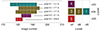 |
Fig. 3. Example of a multichannel (four channel) and multipixel (five pixels) event clustered from individual brightenings into a single nanoflare using the algorithm described in the main text. The left panel illustrates the overlap of brightenings in time. The right panel shows the pixel spatial distribution. The event is not typical and was chosen only to demonstrate the method (single-pixel and single-channel events dominate the nanoflares studied here). Brightening in different channels can also occur in the same pixel. |
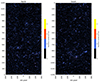 |
Fig. 4. Distribution of the total number of nanoflares in the northern and southern hemispheres. An event visible in several channels simultaneously (multichannel event) is considered as a unique event as well as an event visible only in one channel (single-channel event). |
Based on the data from Table 4, we calculated two parameters:
– The nanoflare rate [events cm−1 s−1],

where N is the number of nanoflares (second column in Table 4), S = 1.60 × 1021 cm2 is the area of the frame (one frame in the northern hemisphere and the second in the southern; see Eq. (1)), and Δt = 3600 s is the duration of observations.
– The nanoflare frequency [events s−1] relating to the entire Sun, including its invisible side:

where S⊙ = 6.09 × 1022 cm2 is the total surface area of the Sun.
The calculated rate and frequency for all the channels are shown in Table 5. The total rate and frequency of all nanoflares are not equal to the sum of the rates and frequencies in individual channels, respectively, because some flares are observed in several channels simultaneously. The percentage shows the proportion of all nanoflares observed in a particular channel. We discuss these results further when we outline our conclusions in Sect. 4.
Nanoflare features.
3.2. Latitudinal distribution of nanoflares and south–west asymmetry
As mentioned above, the search for nanoflares was conducted independently for each channel in the northern and southern hemispheres of the Sun (see Fig. 1). We made no distinction between the northern and southern data when we calculated the rate given in Table 5. Let us now compare the data from different hemispheres and study the dependence of the nanoflare rate on solar latitude.
To study the latitude dependence, we converted the pixel coordinates of nanoflares [x,y] into heliographic coordinates [ϕ,λ], where ϕ is the heliolatitude and λ is the heliolongitude:
where Rpix = 1580.6 is the radius of the Sun in pixels. The nanoflare rate, Pϕ at latitude ϕ was defined as the nanoflare number in interval [ϕ, ϕ + Δϕ] divided by the corresponding area of the Sun, ΔS:

where
Here Rcm = 6.96 × 1010 cm is the radius of the Sun in centimetres, and 300 is the half-width of the studied fragment of the Sun in pixels.
The resulting latitudinal distributions are shown in Fig. 5. We also compared the rate of nanoflares in the northern and southern hemispheres of the Sun and found no significant evidence of asymmetry (see Table 5). The difference in the total nanoflare number between the northern and southern hemispheres is only 4%. For individual channels, the difference can be up to 20%.
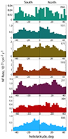 |
Fig. 5. Nanoflare latitudinal distributions. |
3.3. Multichannel study of nanoflares
According to the results shown in Table 5, there are no individual channels that correctly represent the full rate of nanoflares. The maximum individual rate is observed in channels 171 Å and 193 Å, but even there it is only equal to one-third of the full rate (34% and 33%, respectively). The obtained results provide a strong argument in favor of a multiwavelength search and analysis of nanoflares. Therefore, we next compared different channel combinations in terms of their performance for (a) nanoflare retrieval and (b) multiwavelength nanoflare analysis.
The ranking of channels in terms of the nanoflare search efficiency is shown in Table 6. The percentages mean that if we are looking for a nanoflare in these channels, it will be found above the 5σ threshold in at least one of them with the stated probability. A combination of three channels, namely, 171 Å, 193 Å, and 211 Å, makes it possible to detect about 80% of nanoflares. The remaining four channels will increase the nanoflare number only by 20%. Combinations of two channels make it possible to find 50–60% of nanoflares.
Nanoflare search success for different channel combinations.
The results of channels ranking in terms of their effectiveness for multiwavelength analysis are given in Table 7. Here, we considered all the cases where a nanoflare is observed in several (two or more) coronal channels. We excluded channel 304 Å, as it belongs to the transition region. A value of 20% for a pair 171-193, as an example, means that among all the cases when a nanoflare was observed in two channels, in 20% of cases it was this particular combination: 171 Å and 193 Å. For other cases, the ranking was performed similarly. In general, we see that the channels 131 Å, 171 Å, 193 Å, and 211 Å strongly dominate over the others, which is especially noticeable in the right column of Table 7 with the ranking for four-channel combinations. All two-channel and three-channel combinations within this set have approximately equal effectiveness, although the pair “171-193” and the triple set “171-193-211” slightly dominate over the other options.
Channel combination ranking for nanoflare multiwavelength analysis.
3.4. Duration of nanoflares in different spectral channels
The duration of nanoflares as measured using the method described in Sect. 2 (see also Fig. 2) is presented in Table 5. From this point of view, the channels can be ranked as follows: (1) 171 Å, 193 Å, 211 Å, and 304 Å with a duration of ∼(130 − 140)±(55 − 60) s; (2) 131 Å (∼110 ± 50 s), and (3) 94 Å, and 335 Å (∼90 ± (40 − 50) s). Taking into account the large dispersion of measurements, we can conclude that the duration of nanoflares weakly depends on the spectral range. If we still consider the difference to be significant, then we can notice that, in “high-temperature” channels (94 Å, 131 Å, and 335 Å), the nanoflares have a shorter duration than in the other channels. This is consistent with the idea that high-temperature plasma in flares (and nanoflares) has a shorter lifetime than plasma of lower temperature. However, this conclusion should be treated with caution because, in the spectrum of the quiet Sun, the main contribution to the channels 94 Å, 131 Å, and 335 Å comes from ions Fe X, Fe VIII, Mg VIII, and Al X with characteristic formation temperatures of log T ≤ 6.1 (O’Dwyer et al. 2010).
Figure 6 provides additional information on nanoflare lifetime distribution in so-called box-and-whisker form. The white lines mark the median value for each channel (50% of nanoflares are above this level, and the other 50% are below). The boundaries of the boxes show 25% and 75% levels (half of the nanoflares are inside the box), and the edges of the whiskers mark the [5%, 95%] range. Only 10% of nanoflares are outside these boundaries. In general, we see that the majority of nanoflares have a lifetime of less than 5 min in all spectral ranges.
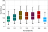 |
Fig. 6. Box-and-whisker plot for nanoflare duration in different spectral channels. The white line is a median value. Boundaries of the boxes are 25% and 75% levels. Whiskers are 5% and 95% levels. |
3.5. Estimation of energy
The thermal energy associated with one pixel can be estimated in the following way (Joulin et al. 2016):
 (2)
(2)
where kB is the Boltzmann constant, and ne, EM, and T are the electron number density, emission measure, and temperature in the considered pixel, respectively. In Eq. (2), V = Aph is the plasma volume, and Ap and h are the area and height of the plasma volume represented by the pixel. Also, q is the factor of volume filling by plasma. In our estimation, Ap ≈ 1.94 × 1015 cm2 and we assume that  and q = 1.
To estimate the energy, we use the dataset consisting of nanoflares found in 131 Å, 171 Å, 193 Å, and 211 Å channels without repetition (if a nanoflare was found in several channels simultaneously, we extract its parameters from one channel only with the priority: 171 Å, 193 Å, 211 Å, and 131 Å). We consider this channel set for several reasons. First of all, it covers the majority of the events found (there are 36 186 events in the dataset). Also, this approach neglects the events visible only in 304 Å as chromospheric events. Moreover, we do not use 094 Å and 335 Å because they are noisy and could have a negative impact on the results of the differential emission measure (DEM) inversion.
Next, we took 131 Å, 171 Å, 193 Å, and 211 Å intensity data to calculate DEM for the profiles of nanoflares in our dataset. To calculate DEM, we used the SITES (solar iterative temperature emission solver) algorithm (Morgan & Pickering 2019) with 31 temperature bins in the temperature range of 0.2–5 MK. The tolerance was set to 5% and the maximum number of iterations was 300. The DEMs found were used to calculate the pixel thermal energies using Eq. (2). These energies were summed if there were several pixels for a nanoflare. We found that the maximum thermal energies are in the range of ∼1023 − 1026 erg, while the difference between maximum and minimum thermal energy during flares falls into the ∼1022 − 1026 erg range.
In addition, we tried a different approach to calculate the thermal energies without any knowledge of h and q, but with the assumption of mean plasma temperature T0 and number density n0. If we assume that plasma consists of n temperature components with temperatures Ti and emissions EMi and all these components are of the same mean pressure ⟨p0⟩ (mechanical equilibrium), then we can rewrite Eq. (2) as:
 (3)
(3)
If assume T0 = 1 MK and n0 = 109 cm−3, then ⟨p0⟩=n0kBT0 = 0.138 dyn cm−2 and, in this case, the maximal thermal energy is in ∼1023 − 1027 erg and difference energy is in ∼1022 − 1026 erg range.
4. Conclusions
In this study, we investigated how the main characteristics of solar nanoflares (their rate, frequency, lifetime, etc.) depend on the spectral range where they are observed. For this purpose, we used quiet-Sun data obtained by SDO/AIA in seven EUV channels (94 Å, 131 Å, 171 Å, 193 Å, 211 Å, 304 Å, and 335 Å) during deep minimum solar activity on 20 May 2019 from 12:00 UT to 13:00 UT (300 images with a cadence of 12 s in each channel).
Using a threshold-based algorithm, we found about 121 000 brightenings above the 5σ threshold, which corresponds to 40 645 nanoflares in the maximum thermal energy range of ∼1023 − 1027 erg calculated using Eq. (3). Most nanoflares (86%) were detected in only one channel. Among the rest, 7% were double-channel events, 2.5% were three-channel events, 2% were four-channel events, 2% five-channel events, and 0.3% were six-channel events. For 0.06% of the nanoflares we observed (24 events), the 5σ threshold was exceeded in all seven spectral channels. In terms of nanoflare size, we obtained the following distribution: 77.7% single-pixel events, 9.7% double-pixel events, 2.9% three-pixel events, and 9.7% covered four or more pixels (half of these, ∼4.6%, covered ten or more pixels).
The integral rate of nanoflares measured in all the spectral ranges (a nanoflare is detected if it exceeds the 5σ threshold in at least one channel) was found to be 3.53 × 10⁻²¹ cm−2 s−1, which corresponds to the frequency of about 215 events s−1 for the entire surface of the Sun, including its invisible side.
Figure 7 shows the distribution of nanoflare frequencies for the different channels compared to the previous single-channel studies shown in Table 1. Due to differences in the instruments and techniques used for nanoflare detection, a direct comparison of the results is limited. However, the results obtained here are in clear agreement with the literature. Furthermore, our study also shows the effectiveness of nanoflare detection using previously unused channels. The probability of detecting a nanoflare depends significantly on the spectral range. The maximum probabilities are observed in the 171 Å (34%) and 193 Å (33%) AIA channels; followed by the 211 Å (24%) and 131 Å (16%) channels. In any case, no single channel can be used to more than one-third of all events. The combination of three channels, namely 171 Å, 193 Å, and 211 Å, allows the detection of ∼80% of all nanoflares. The rate and frequency of nanoflares is roughly independent of the helio-latitude with strong variations (±50%) around the average value. The asymmetry in nanoflare rate between the northern and southern hemispheres of the Sun did not exceed 4%, but could reach up to ∼20% in some channels. In any case, we do not consider this difference to be statistically important. The average duration of nanoflares was 129 ± 59 s. The nanoflares observed in “low-temperature” channels (171 Å, 193 Å, 211 Å) have, on average, longer lifetimes (∼130 s) than those observed in channels with higher temperature response: 131 Å (111 s), and 094 Å and 335 Å (∼90 s). The longest duration is observed in the transition region of the Sun (304 Å): 141 s. We wish to emphasize that, during our study, we excluded all brightenings in channel 304 Å that did not have a counterpart in the EUV coronal channels. This gives us confidence that all the events analyzed in the 304 Å line represent the low-temperature component of coronal nanoflares and do not belong to any type of chromospheric activity. The maximum lifetime of a nanoflare rarely exceeds 3–4 min. We find the probability of detecting a nanoflare with a longer duration to be less than 5% in all the spectral channels. We expect that our study will contribute to a better understanding of the nature of solar nanoflares as multitemperature phenomena and will be useful for interpreting the results of modern multiwavelength studies of small-scale solar activity.
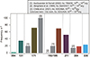 |
Fig. 7. Frequency of nanoflares in different spectral channels given in terms of the total surface of the Sun. |
Acknowledgments
The study was supported by the Russian Science Foundation under the project no. 22-22-00879.
References
- Aschwanden, M. J. 2022, ApJ, 934, L3 [NASA ADS] [CrossRef] [Google Scholar]
- Aschwanden, M. J., & Parnell, C. E. 2002, ApJ, 572, 1048 [NASA ADS] [CrossRef] [Google Scholar]
- Aschwanden, M. J., Tarbell, T. D., Nightingale, R. W., et al. 2000, ApJ, 535, 1047 [Google Scholar]
- Barnes, W., Cheung, M., Bobra, M., et al. 2020a, J. Open Source Softw., 5, 2801 [NASA ADS] [CrossRef] [Google Scholar]
- Barnes, W. T., Bobra, M. G., Christe, S. D., et al. 2020b, ApJ, 890, 68 [Google Scholar]
- Benz, A. O., & Krucker, S. 2002, ApJ, 568, 413 [Google Scholar]
- Berghmans, D., Clette, F., & Moses, D. 1998, A&A, 336, 1039 [NASA ADS] [Google Scholar]
- Boerner, P., Edwards, C., Lemen, J., et al. 2012, The Solar Dynamics Observatory, 41 [Google Scholar]
- Bogachev, S. A., Ulyanov, A. S., Kirichenko, A. S., Loboda, I. P., & Reva, A. A. 2020, Physics-Uspekhi, 63, 783 [NASA ADS] [CrossRef] [Google Scholar]
- Chitta, L. P., Peter, H., & Young, P. R. 2021, A&A, 647, A159 [NASA ADS] [CrossRef] [EDP Sciences] [Google Scholar]
- Erdélyi, R., & Ballai, I. 2007, Astron. Nachr., 328, 726 [CrossRef] [Google Scholar]
- Fludra, A. 2023, A&A, 674, A131 [NASA ADS] [CrossRef] [EDP Sciences] [Google Scholar]
- Hudson, H. 1991, Sol. Phys., 133, 357 [NASA ADS] [CrossRef] [Google Scholar]
- Joulin, V., Buchlin, E., Solomon, J., & Guennou, C. 2016, A&A, 591, A148 [NASA ADS] [CrossRef] [EDP Sciences] [Google Scholar]
- Klimchuk, J. A. 2015, Phil. Trans. Royal Soc. London Ser. A, 373, 20140256 [Google Scholar]
- Krucker, S., & Benz, A. O. 1998, ApJ, 501, L213 [Google Scholar]
- Lemen, J. R., Title, A. M., Akin, D. J., et al. 2011, Sol. Phys., 275, 17 [Google Scholar]
- Massa, P., Emslie, A. G., Hannah, I. G., & Kontar, E. P. 2023, A&A, 672, A120 [NASA ADS] [CrossRef] [EDP Sciences] [Google Scholar]
- Mondal, B., Klimchuk, J. A., Vadawale, S. V., et al. 2023, ApJ, 945, 37 [NASA ADS] [CrossRef] [Google Scholar]
- Morgan, H., & Pickering, J. 2019, Sol. Phys., 294, 135 [NASA ADS] [CrossRef] [Google Scholar]
- O’Dwyer, B., Del Zanna, G., Mason, H. E., Weber, M. A., & Tripathi, D. 2010, A&A, 521, A21 [Google Scholar]
- Ortiz, A., Hansteen, V. H., Nóbrega-Siverio, D., & Rouppe van der Voort, L. 2020, A&A, 633, A58 [NASA ADS] [CrossRef] [EDP Sciences] [Google Scholar]
- Parker, E. N. 1983, ApJ, 264, 642 [Google Scholar]
- Parker, E. N. 1988, ApJ, 330, 474 [Google Scholar]
- Parnell, C. E., & Jupp, P. E. 2000, ApJ, 529, 554 [Google Scholar]
- Priest, E., Chitta, L., & Syntelis, P. 2018, ApJ, 862, L24 [NASA ADS] [CrossRef] [Google Scholar]
- Purkhart, S., & Veronig, A. M. 2022, A&A, 661, A149 [NASA ADS] [CrossRef] [EDP Sciences] [Google Scholar]
- Ulyanov, A. S., Bogachev, S. A., Loboda, I. P., Reva, A. A., & Kirichenko, A. S. 2019a, Sol. Phys., 294, 1 [NASA ADS] [CrossRef] [Google Scholar]
- Ulyanov, A. S., Bogachev, S. A., Reva, A. A., Kirichenko, A. S., & Loboda, I. P. 2019b, Astron. Lett., 45, 248 [CrossRef] [Google Scholar]
- Vilangot Nhalil, N., Nelson, C. J., Mathioudakis, M., Doyle, J. G., & Ramsay, G. 2020, MNRAS, 499, 1385 [NASA ADS] [CrossRef] [Google Scholar]
All Tables
All Figures
|
Fig. 1. Sun in the SDO/AIA 171 Å channel for 20 May 2019 11:59:59 UT. White rectangles denote the areas where nanoflares were searched. |
| In the text | |
|
Fig. 2. Method used to search for nanoflares in the present study. A real nanoflare in channel 171 Å is used as an example. |
| In the text | |
|
Fig. 3. Example of a multichannel (four channel) and multipixel (five pixels) event clustered from individual brightenings into a single nanoflare using the algorithm described in the main text. The left panel illustrates the overlap of brightenings in time. The right panel shows the pixel spatial distribution. The event is not typical and was chosen only to demonstrate the method (single-pixel and single-channel events dominate the nanoflares studied here). Brightening in different channels can also occur in the same pixel. |
| In the text | |
|
Fig. 4. Distribution of the total number of nanoflares in the northern and southern hemispheres. An event visible in several channels simultaneously (multichannel event) is considered as a unique event as well as an event visible only in one channel (single-channel event). |
| In the text | |
|
Fig. 5. Nanoflare latitudinal distributions. |
| In the text | |
|
Fig. 6. Box-and-whisker plot for nanoflare duration in different spectral channels. The white line is a median value. Boundaries of the boxes are 25% and 75% levels. Whiskers are 5% and 95% levels. |
| In the text | |
|
Fig. 7. Frequency of nanoflares in different spectral channels given in terms of the total surface of the Sun. |
| In the text | |
Current usage metrics show cumulative count of Article Views (full-text article views including HTML views, PDF and ePub downloads, according to the available data) and Abstracts Views on Vision4Press platform.
Data correspond to usage on the plateform after 2015. The current usage metrics is available 48-96 hours after online publication and is updated daily on week days.
Initial download of the metrics may take a while.