| Issue |
A&A
Volume 674, June 2023
|
|
|---|---|---|
| Article Number | A131 | |
| Number of page(s) | 10 | |
| Section | The Sun and the Heliosphere | |
| DOI | https://doi.org/10.1051/0004-6361/202245306 | |
| Published online | 13 June 2023 | |
Statistical study of extreme-ultraviolet nanoflares in the quiet-Sun transition region
RAL Space, UKRI STFC Rutherford Appleton Laboratory, Didcot OX11 0QX, UK
e-mail: This email address is being protected from spambots. You need JavaScript enabled to view it.
Received:
27
October
2022
Accepted:
10
April
2023
Abstract
Aims. We carried out a large statistical study of ubiquitous small-scale extreme-ultraviolet (EUV) brightenings in the nanoflare energy range in the quiet-Sun transition region to derive their properties, estimate their contribution to the heating of the solar atmosphere, and compare their numbers to the coronal events published in the literature. This is the first study of this magnitude at temperatures of about 2 × 10⁵ K.
Methods. We applied a numerical method for detecting small-scale transient events in long 1D image time series. We used data recorded by the SOHO Coronal Diagnostic Spectrometer (CDS) in the transition region line O V 62.97 nm (220 000 K) and analysed 702 h of sit-and-stare time series obtained with a cadence of 15.6 s and 50 h with a cadence of 20.5 s in different quiet-Sun areas at a fixed slit position. These data span from 1996 to 2011. This analysis used a different method and a vastly larger number of data than the previous high-cadence CDS study of small events.
Results. We derive histograms of event durations, of the rise and decay time, of the peak intensity and thermal energy, and we obtain a continuous spectrum of their distributions for 117 000 events, spanning the nanoflare energy range with a linear spatial extent of 2−10 arcsec and with durations between 45 s and 40 min. The event peak intensity varied by a factor of 60. We demonstrated that all categories of small-scale events in the transition region are part of a continuum of activity. We obtain a total event rate of 460 s−1 on the entire surface of the Sun. This is more than four times greater than the coronal rate. The maximum value of the duration distribution occurs at 235 s, which is twice the duration of the coronal events. The decay time and rise time difference seen from the shortest to the longest events is symmetrical. We find two event populations: the power law of the smallest events that are confined to one pixel is far steeper for the peak count rates (index of −4.1) and thermal energy (index of −7) than the power law for combined larger events that extend over two or more pixels along the slit (thermal energy power-law index from −2.1 to −3.4).
Conclusions. The power law of the thermal energy of the smallest events, extrapolated to lower energies (picoflares), may provide a huge amount of energy for heating the entire transition region plasma at temperatures of about 220 000 K. An extrapolation of only the flatter power law of the larger events can also account for the entire observed emission.
Key words: Sun: UV radiation / Sun: transition region / Sun: corona / instrumentation: spectrographs / methods: observational / techniques: imaging spectroscopy
© The Authors 2023
 Open Access article, published by EDP Sciences, under the terms of the Creative Commons Attribution License (https://creativecommons.org/licenses/by/4.0), which permits unrestricted use, distribution, and reproduction in any medium, provided the original work is properly cited.
This article is published in open access under the Subscribe to Open model. This email address is being protected from spambots. You need JavaScript enabled to view it. to support open access publication.
1. Introduction
Understanding the processes that heat the quiet-Sun atmosphere remains one of the important questions in solar physics. One of the avenues that was observationally investigated since the advent of high-resolution extreme-ultraviolet (EUV) measurements is the global role of small, short-lived brightening events that are often referred to as nanoflares after Levine (1974) and Parker (1988), who introduced the nanoflare concept theoretically. By definition, the energy range of these events is approximately 1023 − 1026 erg. In assessing their contribution to the heating of the corona, many papers have extrapolated the behaviour of large flares, which show a power law of the peak flare intensity distribution (Crosby et al. 1993). The simple criterion introduced by Hudson (1991) states that the slope of the power law needs to be steeper than −2 for events with energies lower than that of nanoflares (below 1024 erg) to provide the required contribution to the coronal heating. The concept of the event energy distribution and calculations of its slope have been widely adopted in many studies of quiet-Sun nanoflares. The emphasis in the literature has been on coronal events. We therefore briefly summarise the main points from this area to compare them later when we discuss the main focus of this paper, which is the transition region.
Several authors (e.g. Krucker & Benz 1998, 2001; Berghmans et al. 1998; Aschwanden et al. 2000; Parnell & Jupp 2000) studied coronal small events in EUV time series from imaging telescopes on the SOHO and TRACE missions and concluded that the observed events in the nanoflare range do not have enough energy to explain the heating requirements of the quiet-Sun corona, 3 × 10⁵ erg cm−2 s−1 (Withbroe & Noyes 1977). Krucker & Benz (1998) and Parnell & Jupp (2000) investigated various scenarios of extending the power law to lower energies, and estimated that the heating events would need to extend to energies as low as 1019 − 1021 erg to provide the required energy. Events in this energy range (picoflares), if they exist, have such a small magnitude that they are drowned out by the statistical noise and are currently undetectable.
More recent observations by the Solar Dynamics Observatory (SDO) AIA instrument used a much faster image cadence than these early studies. Chitta et al. (2021) analysed 171 Å images with a cadence of 12 s from SDO/AIA in the quiet Sun and obtained the statistics of short-lived (100 s) EUV bursts at coronal temperatures. Purkhart & Veronig (2022) derived power-law energy distributions of nanoflares, also using AIA images with a cadence of 12 s. They obtained impressive statistics and an extension to higher energies up to 1029 erg. Qualitatively, the conclusions from the earlier studies have not changed.
After the launch of the Solar Orbiter mission (Müller et al. 2020), Berghmans et al. (2021) reported the detection of the smallest coronal events registered so far (called campfires) in Solar Orbiter EUI images at 17.4 nm and derived their first characteristics. This is now a flourishing area of research.
Another domain with a pronounced short-term variability in the EUV emission is the solar transition region in the temperature range between 30 000 K and 600 000 K. It is characterised by significant variability in the EUV spectral line intensities on short temporal and small spatial scales. The transition region, in particular at temperatures of about 220 000 K, is the focus of this paper.
Several categories of brightening events in the quiet-Sun transition region were discussed in the literature. We describe them below.
(1) Small, short-lived events with most frequently occurring durations between one and several minutes, sizes from 2″ × 4″, and energies in the nanoflare range (1024 − 1027 erg) were observed in the He II 30.4 nm images from SOHO/EIT. They are emitted at low transition region temperatures of approximately 5 × 10⁴ K (Berghmans et al. 1998). They were also detected by Harra et al. (2000), who analysed a two-hour time series of a spectral line of O V 62.9 nm emitted at 2.2 × 10⁵ K. This was recorded by the SOHO Coronal Diagnostic Spectrometer (CDS). These events are similar to the coronal brightenings mentioned earlier.
(2) Long-lived events called blinkers (Harrison 1997) are spatially extended and have been studied both individually and statistically (Bewsher et al. 2002). Their lifetime range is 400 − 2400 s, with a mean value of 960 s. The intensity enhancements are typically up to 80%, but can be higher occasionally.
For completeness, we mention a rare type of bright features in the transition region, called beacons. They were reported by Fludra et al. (2021) based on Solar Orbiter observations made with the SPICE instrument (SPICE Consortium 2020). Their intensities are 15−30 times higher than the average quiet-Sun intensity, with lifetimes longer than two hours. They appear to be connected to the coronal bright points. Due to their extreme brightness, rare occurrence, and long lifetimes, they lie at the extreme end of the event frequency distribution, beyond the range of events of interest to this paper.
Here, we detect the small-scale events on all temporal scales, but are mainly interested in those events listed in point (1) above that have similar sizes, energies, and behaviour as the coronal nanoflares summarised earlier. The importance of studying the brightening events in the transition region has been emphasised by Hansteen et al. (2015) and Guerreiro et al. (2015), who calculated 3D magnetohydrodynamic (MHD) models of the quiet-Sun corona and carried out statistical studies of the heating events. According to these models, the location of the heating events is in the low transition region at heights between 1.5 Mm and 3 Mm. This provides additional motivation for deriving more precise observational characteristics of high-cadence observations of the transition region lines for a future comparison with models.
The CDS (Harrison et al. 1995) on board SOHO can make a unique contribution to this study using the bright spectral line of O V 62.9 nm at a temperature of 220 000 K. Between 1996 and 2011, we obtained more than 700 h of the O V line time series in quiet-Sun areas, and we use them in this paper to provide a precise statistical determination of event characteristics such as their frequency, durations, rise and decay times, and thermal energy distribution.
This can fill the gap in the relatively scarce observations of the short-term variability at mid-transition region temperatures. That we use many more hours of SOHO/CDS time-series observations than heretofore published in the literature, with a very good temporal resolution of 15 s, will increase the accuracy of the measurements of the transition region variability and the characteristics of the brightening events. We also use a different detection method with a stringent detection threshold, which significantly affects the numbers of detected events and eliminates noise fluctuations.
Further motivation for the study of sit-and-stare spectrometer time series comes from the Solar Orbiter mission, which carries the EUV spectrometer SPICE (SPICE Consortium 2020; Fludra et al. 2021) on board. This instrument predominantly observes transition region lines. SPICE can use an even shorter cadence (5 s) of very bright spectral lines and has the potential to further increase our understanding of the small-scale brightenings and their nature. The results of this paper will provide guidance in defining the SPICE observing programme.
Section 2 describes the data, and Sect. 3 describes the method. The results are presented and discussed in Sects. 4 and 5.
2. Instrument and data
2.1. Observing studies
The CDS on board SOHO observes EUV spectra from the solar transition region and corona. The normal incidence spectrometer (NIS) of the CDS uses an intensified CCD camera, consisting of a microchannel plate coupled to a phosphor screen and a CCD. A typical data product of the NIS spectrometer are EUV spectra in two wavelength bands, 30.8−38.1 nm (NIS1) and 51.3−63.3 nm (NIS2). In this paper, we used a 4″ × 240″ slit and either a single or double binning of pixels along the slit, resulting in pixel sizes of 4″ × 1.68″ or 4″ × 3.36″, respectively. Occasionally, only the central half of the slit (120″) was used, and the different parameters: single- and double-binning, partial slit length, and different exposure times were later accounted for when the normalised statistics of the events were calculated.
Our main CDS observing study is called SAS250W, with double-binned pixels. During one observing sequence, the slit was pointed to a selected target in a quiet-Sun area, and a series of 250 exposures was made at the same spatial position, each with the same exposure time of 10 s. This constitutes one study that took about 65 min (after each 10 s exposure, there is a delay of 5.65 s before the next exposure is taken). This study unit was then repeated several times (between 3 and 14), creating a time series with a total duration between 3 and 15 h. These time series were scheduled on 76 dates throughout the mission until 2011, providing 702 h of observations. In all analysed datasets, CDS maintained a fixed pointing on the solar disk, such that all solar features moved across the field of view of the 4 arcsec slit due to solar rotation.
The second, auxiliary study is called NTBRMDI2, with a single-binning of pixels along the slit, and an exposure time of 15 s, resulting in a cadence of 20.5 s. The basic unit of this study was a series of 30 exposures, repeated several times (a range of 6−22). It was run mostly at the beginning of the SOHO mission, and a total of 50 h of observations from 1996 to 1997 were selected. We used it occasionally to illustrate the data or verify some of the results. Both studies record line profiles of the bright line of O V at 62.9 nm, emitted at a temperature of approximately 220 000 K.
Figure 1 shows an example of the distance-time image of a time series from the NTBRMDI2 study over five hours. We chose this study for illustration because it has the best spatial resolution. Large, bright structures that represent the network dominate visually. However, as we show below, the many smaller and fainter features form the peak of the intensity and energy histogram.
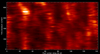 |
Fig. 1. Example image of the time series of the O V 62.7 nm line intensity along the slit from the NTBRMDI2 study. The pixel size along the slit is 1.68″ (single binning). The time step of each exposure number along the Y-axis is 20.5 s. The duration of this series is five hours. |
The images from the SAS250W series are similar, except that they have double-binned pixels along the slit (i.e. along the X-axis). The SAS250W data set is much larger, and we concentrate on its analysis in this paper.
Figure 2 shows examples of the temporal variation in intensity of the O V line in selected pixels from Fig. 1. The peaks in these light curves are the events that are detected and analysed in this paper.
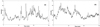 |
Fig. 2. Example light curves (i.e. intensity in units of [counts per exposure]) of the time series from Fig. 1. (a) Left panel: in pixel 70. (b) Right panel: in pixel 120. The intensity scale in panel (b) is half of the scale in panel (a). Each peak in these light curves constitutes an event. |
2.2. Calibration
The CDS/NIS spectrometer was calibrated on the ground and in flight (Lang et al. 2002). The data were processed using the CDS calibration routine vds_calib, which converts signal into counts per pixel per second, denoted as Ivds. We fit the observed O V line profiles with either Gaussians (for observations obtained prior to the loss of SOHO attitude control in June 1998) or broadened Gaussians after the SOHO recovery (Thompson 1999) to calculate the integrated line intensities.
During the SOHO mission, when the same positions on the CDS/NIS detector were repeatedly exposed to strong lines, the NIS microchannel plate experienced a burn-in effect, that is, it gradually lost sensitivity at these positions. This effect was monitored throughout the mission, and appropriate correction has been derived and is implemented in the standard CDS analysis software. The long-term NIS calibration was re-analysed and improved by Del Zanna & Andretta (2015). Their sensitivity correction was applied to the data before the event detection analysis. We further comment on this in Sect. 3.
3. Method
Several event detection methods were used in the literature (e.g. Berghmans et al. 1998; Harra et al. 2000; Parnell & Jupp 2000; Aschwanden et al. 2000). We selected the approach of Bewsher et al. (2002), which was originally designed for blinkers. It analyses the time history of each pixel separately (e.g. in Fig. 2) and gives a good degree of control over the detection parameters: event peak, event start and end time, and statistical detection threshold. Their prescription for a three-stage method was used by Haigh (2006) to write a code from first principles, optimised for long time series of 1D images along the spectrometer slit. This detection software was applied in this paper.
The event detection procedure is separated into three stages: detecting events in individual pixel light curves, grouping adjacent pixel events occurring at the same time, and, finally, determining the start and end of the total event. The grouping results in events with different lengths along the slit: one-pixel events, two-pixel events, and so on.
For an event peak to be statistically significant, the difference in its intensity above the background must be greater than nσ, where σ is the statistical error of the nearby background intensity. We assumed n = 3 here. As illustrated in Sect. 5, when the value of n is too low, the noise fluctuations are identified as real events, and this significantly increases the number of detected events.
The error σ was initially calculated from the formula given by Thompson (2000). Before applying it, we multiplied the intensity count rates Ivds [counts pixel−1 s−1] produced by the vds_calib routine by the exposure time to obtain the line counts/pixel, Ic. However, we realised that after applying the long-term burn-in correction, the number of detected events significantly increased with time, doubling the event rate in the SAS250W study by 2011. The reason was that while the burn-in correction restored the line intensities, it did not remove the increased noise in the intensities present in the data before the correction. We therefore introduced an additional empirical factor bc/2.3, where bc is the burn-in correction, and calculated  , which gives us a flat long-term event rate and removes the false events created by noise from 1999 onward.
4. Results
4.1. Event detection
Figure 3 shows an example of all events detected in the time series from Fig. 1. Each white box is one event. The box size along the X-axis is equal to the number of pixels in that event, that is, the event length. The size along the Y-axis is the event duration. We illustrate this with an example of the NTBRMDI2 series because it has the best spatial resolution of 1.68″ pixels. These patterns were derived for all 76 dates when the SAS250W study was run. The results are given below.
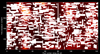 |
Fig. 3. Events detected in the time series from Fig. 1. The size of each box in the Y direction is from the event start time to the event end time. The size of each box in the X direction includes all pixels grouped as one event. See text for details. |
4.2. Event durations
The histogram of event durations from the SAS250W study is presented in Fig. 4. The distribution to the right of the peak decays exponentially. The lower curve represents one-pixel events.
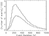 |
Fig. 4. Distribution of the event durations from the SAS250W study. The lower curve represents one-pixel events. The vertical scale has been divided by 1000. |
The distribution shows that the duration of most events exceeds 60 s and extends up to 2500 s (the timescale in the figure was truncated at 1000 s). The distribution peaks at 235 s and is quite flat within ±15 s. It then decays exponentially. The durations of one-pixel events also peak at 235 s.
We also compared the event rise time (the initial increase in intensity) and decay time (the following decrease in intensity) of the brightenings. Figure 5 shows that the distribution of the difference between the decay time and rise time is approximately symmetrical, especially between (−100, 100) s. It centres on a time offset of +15 s. Any model explaining the origin of these events would need to explain this property.
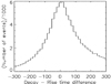 |
Fig. 5. Distribution of the difference between the decay and rise time of the events. Only a small offset of +15 s is present. The vertical scale has been divided by 1000. |
4.3. Event rate
We detected 117 000 events in 702 h of the SAS250W time series per slit area of 4″ × 240″. This gives an average event rate of 0.046 events per second per slit area.
Table 1 shows the event rate for one-pixel, two-pixel, and three-pixel events and their conversion to the event rate on the whole surface of the Sun,  . These conversions were calculated assuming that the event width in the direction perpendicular to the slit is the same as the event length along the slit. The global rate on the whole solar surface is therefore approximately 460 events s−1.
Event rates (s−1) for different event lengths (3.36″ pixels).
Comparing the birth rate of events in the transition region with the rate in the corona reported in papers cited in Sect. 1, we find four times more events in the transition region. This gives a quantitative comparison of the variability in the two domains on small spatial and temporal scales.
To illustrate that different event detection methods can give different results, we compared our rates with the rate obtained by Harra et al. (2000) in one NTBRMDI2 observation. They detected a total number of 1125 events during a 1 h 53 m series, giving an average of 0.16 events per second per 4″ × 240″ slit area. This is approximately three times more events than were detected by our method (we detected 340 events in the same time series).
This can be explained by different methods and detection criteria: We assumed a 3σ threshold above the local background, while Harra et al. (2000) assumed a 10% increase above the background. Since the histogram of the background, both in this particular series and in other series we analysed, peaks at a level of about 100 counts, this suggests that Harra et al. (2000) detected events approximately above 1σ threshold. This would explain the much greater number of events in their study.
In contrast, Berghmans et al. (1998) reported a total full-Sun event birth rate of 14.4 s−1 using a 3σ threshold in the He II 30.4 nm SOHO/EIT images. This rate is a factor 30 lower than what we obtained from the O V 62.9 nm line. The He II line is emitted at temperatures of about 50 000 K, while the O V line is emitted at about 220 000 K. Due to the difference in cadence (66 s for EIT, 15 s for CDS), EIT might be missing some of the shortest-duration events. However, it is generally thought that the transition region at about 200 000 K is the most dynamic region of the solar atmosphere. Therefore, the large difference between the number of the O V events in this paper and the He II events in Berghmans et al. (1998) may be a real property of the solar atmosphere.
4.4. Intensity distribution and thermal energy
Figure 6 shows the histogram of event peak intensities, Ieve (counts per event area per second). The top curve is a global distribution of all events, represented by a power law with a slope of −2.2. The lower curve is the distribution for one-pixel events. Its power law has an index of −4.1. This shows for the first time that one-pixel events have a different power-law index than larger events.
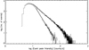 |
Fig. 6. Distribution of the peak event intensity from the 702-h SAS250W time series. The power law fit to the top curve has a slope of −2.2. Events confined to one pixel are overplotted below, with a slope of −4.1. |
The thermal energy, Eth [erg], of a brightening event observed inside the slit is given by
 (1)
(1)
where the event volume V = W × L × D, W = 4″ × 7.2 × 107 cm is the slit width, L [cm] is the event length along the slit, and D [cm] is the line-of-sight depth of the plasma involved in the brightening event. f is the filling factor, that is, the ratio of the actual volume occupied by the plasma to the assumed event volume V. kB is Boltzmann’s constant, and Te is the electron temperature of the plasma in Kelvin, taken at the peak of the emissivity function of the O V ion (220 000 K). Ne is the electron density.
The electron density Ne over volume V is typically estimated from the equation for the line intensity. First, we converted the event countrate Ieve from Fig. 6 into a calibrated intensity Inis in photons cm−2 s−1 ster−1, as would have been derived by the CDS calibration routine nis_calib,
 (2)
(2)
where the factor 2.5 × 10¹¹ is for the SAS250W study with 3.36″ pixels. For the NTBRMDI2 study, with 1.68″ long pixels, this factor is 5 × 10¹¹. Lpix is the event length in integer pixels (1, 2, 3 and so on) along the slit. Subsequently,
 (3)
(3)
where AO = 7.7 × 10⁻⁴ is the absolute coronal abundance of oxygen (Feldman 1992, see also Fludra & Schmelz 1999 for a discussion), and D is the assumed depth along the line of sight. The G(T) function [cm3 s−1] was obtained from the ADAS package (Summers et al. 2006). We assumed that the transition region plasma is not isothermal, but has a constant differential emission measure over the narrow temperature range spanning the shape of the G(T), between log(T) = 5.1 and 5.4. Then we approximated G(T) with its average over this temperature interval, Gave = 0.38G(Tmax), where Tmax = 220 000 K is the temperature at which G(T) reaches the maximum value.
Equation (3) gives us the product  . We discuss the value of f in Sect. 4.6. Assuming for the time being f = 1, we calculated the average electron density Nav over the full volume V.
The last quantity needed for this calculation is the line-of-sight depth, D. We tested three cases: (1) D is proportional to the length L of each brightening. (2) The second assumption was a constant depth equal to the length of the pixel (D = 3.36″ for the SAS250W study). (3) The third assumption was that the depth is inversely proportional to the event length, D ∝ 1/L. This may be counter-intuitive and possibly unphysical, but produced a thermal energy histogram without the dip between one-pixel events and ≥two-pixel events (Fig. 7c). Therefore, we included this option to illustrate how it affects the thermal energy.
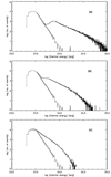 |
Fig. 7. Distribution of the event peak thermal energy for the SAS250W data set for a temperature of 220 000 K, assuming the depth D of the O V emission along the line of sight. (a) Equal to the event length along the slit (top panel). (b) Constant, equal to 3.36″ (middle panel). (c) Proportional to 1/length (bottom panel). The straight lines in all panels are power-law fits obtained separately for the population of one-pixel events (on the left) and the population of longer events with two or more pixels (on the right). The power index is given in Table 2. The energy along the X-axis is an upper limit derived with f = 1 (see Sects. 4.4 and 4.6 for a discussion). |
Figure 7 shows the histograms of thermal energy for these three cases in the range 1023 − 1025 erg. We note that because we assumed f = 1, this is an upper limit on thermal energy and is discussed further in Sect. 4.6.
The shape of the power law changes with different assumptions for the depth. In each panel, events with one-pixel length produce the first and largest peak, with a very steep slope of −7. Larger events produce the second peak with a power-law slope of between −2.16 and −3.4 (Table 2). This large difference between the power-law indices suggests that one-pixel events come from a separate population of events and might be created by a different mechanism than larger events.
Power-law index of thermal energy distributions.
We point out, however, that the duration distribution of one-pixel events (Fig. 4) follows a similar curve as that for all events. Therefore, one-pixel events are not limited to short durations.
4.5. Reduced pixel size: NTBRMDI2 study
In this section, we summarise results from the NTBRMDI2 study with single-binned pixels, 4″ × 1.68″. We denote these pixels with the letters sb (for single-binned), added after the number of pixels. Therefore, one-sb-pixel events arise from half of the pixel length of one-pixel events in the previously discussed SAS250W study. Figure 8 shows the intensity count rates and energy distributions obtained from 50 h of the NTBRMDI2 series. The distribution of one-sb-pixel events in Fig. 8 is shown on the far left, two-sb-pixel events form the next peak to the right, and the combined ≥two-sb-pixel events form the flatter power law on the far right. The first two curves combined, one-sb-pixel and two-sb-pixel, are equivalent to one-pixel events from Fig. 7.
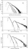 |
Fig. 8. Results from a 50-h series of the NTBRMDI2 study with single-binned pixels, 4″ × 1.68″. (a) Distribution of the peak event count rates per event area (top panel). (b) Distribution of the peak thermal energy, assuming the depth of the O V emission along the line of sight to be equal to the event length along the slit (middle panel). (c) Distribution of the thermal energy, assuming a constant depth along the line of sight, D = 1.68″. In all panels, the curve on the far left shows one-pixel events, the middle distribution is for two-pixel events, and the distribution on the far right shows ≥2-pixel events. The straight lines in all panels are power-law fits obtained separately for each event population. The energy along the X-axis in panels (b) and (c) is an upper limit derived with f = 1 (see Sects. 4.4 and 4.6 for a discussion). |
The total number of events in this series is 8764, which gives an average event rate of 0.048 events per slit area per second. There are 2996 one-sb-pixel events and 1790 two-sb-pixel events.
The statistical quality is lower because the observations lasted only for 50 h, as compared to 702 h in the SAS250W series, but it demonstrates that when the pixel size is reduced by half, 63% of count rates from the original one-pixel events move to the smaller one-sb-pixel events. The thermal energy of one-sb-pixel events has a power index of −5.7.
The middle and bottom panels b and c in Fig. 8 use different assumptions regarding the line-of-sight depth: proportional to the event length along the slit, and a constant depth of D = 1.68″, respectively. This is similar to the top and middle panels a and b of Fig. 7. In studies of coronal nanoflares, the first assumption is most common. It might also be correct for low-lying loops in the transition region, but for the emission arising from the footpoints of the high coronal loops, the second assumption seems more plausible. A further comparison with the SAS250W study is made in Sect. 5.
4.6. Real electron density
In the previous sections, we used estimates of the average electron density that were obtained for a filling factor f = 1. The only way to derive the true electron density Ne in the solar atmosphere is from ratios of density-sensitive lines. Rao et al. (2022) analysed density-sensitive O IV lines observed in the quiet Sun by the SUMER spectrometer on board SOHO and by IRIS. They derived a scatter of electron densities between 109 cm−3 and 3 × 1010 cm−3, with averaged values of 4 × 109 cm−3 from SUMER and about 1010 cm−3 from IRIS. The authors emphasised that the O IV lines are very weak, and it has been notoriously difficult to reliably measure their intensities both in previous studies with the HRTS instrument and in their analysis of SUMER and IRIS data (Rao et al. 2022).
The peak formation temperature of the O IV lines is 1.2 × 10⁵ K, which is about a factor of two lower than the temperature of the O V line studied in this paper. Therefore, assuming a constant pressure in the transition region plasma, we can expect a similar scatter of densities at an O V temperature (2.2 × 10⁵ K), with an average density lower by a factor of two, that is, between 2 × 10⁹ and 5 × 109 cm−3, using the SUMER and IRIS averages as a possible range.
The product  that we derived from Eq. (3) is in the range 8 × 10⁷ to 4 × 108 cm−3, with an average value of 2 × 108 cm−3 for D = 3.36″. This is 10 to 25 times lower than the average densities for O V temperatures we estimated from Rao et al. (2022). This gives an estimate of f = 0.01 − 0.0016.
Rao et al. (2022) also calculated the path length along the line of sight for O IV temperatures, using their derived densities. These high densities give very short path lengths. Most of them scatter between 1 and 100 km, with typical values of a few tens of kilometres. Even shorter path lengths were derived from the HRTS instrument by Dere et al. (1987). This means that the structures are very sparse within the pixel area and are so thin that they cannot be resolved. Therefore, the filling factor is very small, and the path length does not represent the true length of the structures.
Comparing the values of Rao et al. to one of our assumptions for D = 3.36″ = 2400 km, we derive typical filling factors f of about 0.01 to 0.02. This is somewhat higher than those based on densities in the preceding paragraph.
Using the product  we derived from Eq. (3), the thermal energy in Eq. (1) can be written as
 (4)
(4)
The remaining unknown parameter is  at the end of Eq. (4), hence the actual thermal energy scale may be up to 10 − 25 times lower than displayed in Figs. 7 and 8b, c.
However, whether these short path lengths (and therefore the small filling factors) are always applicable to the nanoflare events we studied is not known and would require direct density measurements inside nanoflares. For this reason, we treat the thermal energy range displayed in Figs. 7 and 8b, c as an upper limit, with the understanding that the true thermal energy may be an order of magnitude lower.
5. Discussion
We have carried out a unique analysis of small-scale brightenings in the nanoflare range in the quiet-Sun transition region using a total of 702 h of the SAS250W time series spread over 76 different areas on the Sun, and 50 h of the NTBRMDI2 series from 16 areas on the Sun. These studies have a very good temporal resolution of 15.5 s and 20.6 s, respectively. The first study provides low statistical errors due to the length of the series. It can simultaneously detect all durations and linear sizes of small-scale events considered previously as separate categories in the literature. It also provides nanoflare characteristics at temperatures of 220 000 K that were not observed with previous instruments. The results of this analysis in Fig. 6 show that judging from the top curve, all event categories appear to form a continuous spectrum of transition region activity, represented by one power law of intensity count rates that vary by a factor of 60 at the event peak. The event durations also show a continuous distribution. This possibility was discussed by Berghmans et al. (1998) and Harrison et al. (2003). We note that only 35% of the events along the slit have sizes ≥2 pixels. The majority, 65%, are one-pixel events. These fractions on the solar surface become 22% and 78%, respectively.
The maximum value of the duration distribution occurs at 235 s, which is twice the duration of the coronal events (Chitta et al. 2021; Purkhart & Veronig 2022). The approximate symmetry between the rise and decay time (Fig. 5) is qualitatively similar to the symmetry in blinkers (Bewsher et al. 2002). The average rise and decay times of blinkers were much longer, 8 min, and their numbers on the Sun are 20 times lower (they are concentrated near the end of the scale in Fig. 4). Nevertheless, the similarity in the relative behaviour of the rise and decay times strongly suggests that the process causing the temporal evolution is the same for events of all sizes and lifetimes in the transition region at 2 × 10⁵ K.
Figures 6 and 7 show that the smallest events, confined to one pixel, constitute the peak of the distribution and have a much steeper power law than larger events. The important discovery here is that we found two populations of small-scale events. Events with a length of two or more pixels in the SAS250W study have a power law of the thermal energy with a power index of −2.2, approximately the same as for coronal events derived in many papers studying small-scale events in the corona. This similarity between the two domains is striking. We suggest that these events are driven by the typical interactions of magnetic fields in network structures with sizes that can be resolved by CDS and other instruments. The other population of events that we see so clearly for the first time, with a spatial size that is contained in one CDS pixel, has a power-law index of −7. The thermal energy of these one-pixel events rises very steeply towards lower energies and might heat the transition region on the smallest scales in locations in which no events are detected with current instruments. The mechanism creating most of these smallest events might be different and might arise from MHD turbulence inside the magnetic loops (Jafari et al. 2021). When trying to explain the nature of these brightenings, we need to remember that we observe them in a narrow temperature range around 2.2 × 10⁵ K. It seems likely that they are due either to density or the filling factor enhancements, as found for blinkers (Bewsher et al. 2002).
The power law in Fig. 6 peaks and does not rise further towards lower count rates because of the 3σ detection criterion. If this criterion were lowered, many more faint events would be detected, which would be indistinguishable from statistical noise, however. Future observational efforts should therefore concentrate on improving the sensitivity and spatial resolution of instruments to detect the population of picoflares on spatial scales smaller than 500 km. The observations by Berghmans et al. (2021) are a step in this direction.
The area in the distance-time plot that is covered by all events (i.e. the area of all white boxes, e.g. those in Fig. 3) is 40% of the total area of 240″ × 702 observation hours. However, the total intensity of all events, integrated over their light curves, is only about 19% of the total intensity in the O V line in the entire series. The remaining emission comes from a slowly varying background, either under the event light curves or in less active, event-free areas. We can pose the question whether this dominant background intensity may arise entirely due to events that are smaller than nanoflares.
Pauluhn & Solanki (2007) presented an alternative approach to the analysis of nanoflares in the transition region that fits this situation. They postulated that the entire emission coming from the transition region might be due to events at nanoflare or lower energies. Instead of detecting individual events, they derived the observed radiance distributions from SOHO/SUMER spectral line intensities and compared them to radiance distributions simulated under several different assumptions about the nanoflare characteristics. Ultimately, this also leads to the concept of extending the nanoflare power law to lower energies, but with different observational constraints (i.e. radiance distributions).
The question whether nanoflares can heat the entire corona, when taken literary as pertaining to events with energies limited to approximately 1023 − 1027 erg, has been answered negatively in all coronal studies. That they are insufficient is plain from the coronal images (e.g. Fig. 6b in Parnell & Jupp 2000) and from energy considerations.
Parnell & Jupp (2000) estimated that to provide the required energy to heat the quiet-Sun corona, 3 × 10⁵ erg cm−2 s−1 (Withbroe & Noyes 1977), the power law would need to extend down to at least a few × 1021 erg, or even as low as 1019 erg, depending on the definition of the line-of-sight depth and the assumed detection threshold (e.g. 2σ or 3σ). A similar estimate was made by Purkhart & Veronig (2022), suggesting that the power law they derived would need to extend as low as 5 × 10²⁰ erg to balance the total energy loss of the corona.
We obtain the same answer to the question whether nanoflares can explain all transition region emission in the O V line around temperatures of 2.2 × 10⁵ K. In our time series in Fig. 3, the detected nanoflares occupy less than half of the image area, and their total intensity is 20% of the total O V emission. Nanoflares heat themselves, but they do not heat the areas from which they are absent.
When exploring an extension of the transition region power laws to lower energies, we have two choices. First, we can extend the power law of one-pixel events in Fig. 7, using Eq. (18) from Parnell & Jupp (2000) to calculate the additional power per unit area. Due to the steepness of the one-pixel power law (power index of −7), reducing the lower energy limit Emin merely by a factor of 3 increases the total energy by a factor of 50. Reducing it by another factor of ten increases the total power by five orders of magnitude. This is far more than needed.
Second, we also need to consider the possibility that the steep power law of one-pixel events does not extend so steeply to lower energies, but their energy distribution remains a bell-shaped curve. We can partially test this by comparing the distribution of one-pixel events from the SAS250W series (Sects. 4.1–4.4) with one-sb-pixel events from the NTBRMDI2 series (Sect. 4.5).
Figure 8 shows that reducing the pixel size by half moved the distribution of one-pixel events farther to the left and moved its peak higher, so that these events still constitute 34% of all events. Their power-law index remains steep, with an index of −5.7, but their vertical offset was significantly less than the extrapolation of the original one-pixel events power law. Instead, this offset seems to follow approximately the flatter power law for all events. We can conjecture that a further reduction of pixel sizes would repeat the above pattern.
In this case, a further extension to lower energies would be similar to the coronal case. Extending our power law of the intensity count rates from Fig. 6 for ≥two-pixel events (power index of −2.2) to intensities lower by a factor of 500 than the current lowest values would increase the total integrated intensity by a factor of 5, accounting for all the emission in the O V line (i.e. the nanoflares plus background). This translates into extending the thermal energy from Fig. 7 to energies lower by approximately a factor of 20. Therefore, picoflares can explain the entire transition region emission for sufficiently low energy values.
The difference between the studies of 2D coronal images and 1D time series of the transition region emphasizes different visual aspects of the same problem: (1) In the corona, after detecting and eliminating all events, the researcher is left with a large part of the image in which no events have been found. These areas without events still need a source of heating. (2) In our paper, after detecting a large number of events in the time series of the line intensity, we are left with some parts of the series without events, but also with a substantial, slowly varying background from which the small events arise. The heating that gives rise to both of these background emissions needs an explanation.
These are two facets of the same problem. In both cases, millions of energy releases at the pico/femtoflare range can be postulated to locally provide the required additional heating, and their hypothetical existence agrees with the power laws of nanoflares extrapolated to lower energies. Obtaining the proof of the existence of the invisible pico and femtoflares is now one of the most important goals.
One item that remains to be clarified is the scale of the thermal energy. The results from Sect. 4.6 show that the filling factor is much lower than one, approximately f ≈ 0.01. In this case, the thermal energy scale would be reduced by a factor of ten (Eq. (4)). The exact reduction cannot be easily established because of the large scatter of the values presented by Rao et al. (2022) and the possibility that the nanoflare event characteristics might differ from those of the rest of the typical transition region structures. Hence we elected to show the upper limit of the energy scale in Figs. 7 and 8b, c for f = 1, and we emphasise that an offset to lower energies by a factor of ten is likely. This offset affects the energy we ascribe to the events, but it does not change the rest of conclusions.
Finally, we need to address the question to which degree the transition region is a separate domain from the corona. Some emission certainly comes from near the footpoints of the coronal loops, while other emission is confined to the transition region temperatures and small loops that do not reach the corona. It was suggested by Feldman (1983) that the part of the solar atmosphere between 4 × 10⁴ and 2.2 × 10⁵ K is largely independent of the corona and most of that transition region emission was produced by unresolved fine structures that are not connected to the corona.
Dowdy et al. (1986) also proposed that most of the cool transition region emission originates in low-lying network loops that are magnetically insulated from the corona. Spadaro et al. (2006) carried out simulations using “transient, nanoflare-level heating localized near the chromospheric footpoints of small loops”. Their results show that the emission at temperatures well below 106 K mostly originates from low-lying cooler structures.
Our measurement that the brightening events in the transition region exceed the number of coronal events four times agrees with the ideas above.
6. Conclusions
We have determined the statistical properties of small-scale brightenings at the low end of the nanoflare energy range, 1022 − 1024 erg in the quiet-Sun transition region using 702 h of time series of the O V 629.7 Å line intensity recorded by the SOHO/CDS instrument. We detected 117 000 events over the 4″ × 240″ slit area, using 76 time series with a cadence of 15 s and 3−15 h duration. These brightenings are due either to density or the filling factor enhancements. This is the first study of the transition region variability at this magnitude and uses a stringent 3σ event detection criterion.
We derived a global frequency for the small-scale events of 460 s−1 for the quiet-Sun transition region from the entire solar surface. This is more than four times higher than the coronal rate of small events quoted in the literature.
The duration of the most frequently occurring events is about 235 s ± 15 s. This is twice the value for coronal events.
The distribution of the difference between the decay and rise time is nearly symmetric around +15 s in the (−100 s, 100 s) interval.
We discovered that there are two event populations: The smallest events contained inside one CDS pixel form a separate population with a much steeper power law.
When one-pixel events are analysed separately, their peak count rate power law has an index of −4.1. Larger events have a power law with an overall index of −2.2.
The thermal energy of one-pixel events has the steepest power law with an index of −7, while larger events have a power-law index between −2.15 and −3.4, depending on different assumptions of their line-of-sight depth.
The scale of the derived thermal energy depends on the assumed area filling factor f. Using the common assumption made in the past of f = 1 and the line-of-sight extent of the structures D ≈ 2000 km gives the energy range 1023 − 1025 erg. However, the high electron densities and very short path lengths reported in the literature from density-sensitive lines suggest f ≈ 0.01, reducing the thermal energy by approximately an order of magnitude to 1022 − 1024 erg.
The detected nanoflares account for 20% of the observed emission in the O V line. The remaining background intensity can be explained by extending the energy range by at least an order of magnitude and postulating the existence of unresolved picoflares. Picoflares are viable candidates for heating the quiet-Sun transition region areas in which no nanoflares have been detected, in a similar way as was demonstrated in the literature for the coronal emission.
Acknowledgments
This work was supported by the UKRI Science and Technology Facilities Council (STFC). Data supporting this paper are openly available from the SOHO Science Archive at https://soho.nascom.nasa.gov/data/archive/. SOHO is a project of international cooperation between ESA and NASA. The CDS instrument was built and operated by a consortium led by the STFC Rutherford Appleton Laboratory and including the UCL Mullard Space Science Laboratory, the NASA Goddard Space Flight Center, Oslo University and the Max-Planck-Institute for Extraterrestrial Physics, Garching. The operations of the CDS instrument between 1996 and 2014 were supported by PPARC, STFC and the UK Space Agency. The author thanks Douglas Haigh for writing the event detection software.
References
- Aschwanden, M. J., Tarbell, T. D., Nightingale, R. W., Schrijver, C. J., & Title, A. 2000, ApJ, 535, 1047 [NASA ADS] [CrossRef] [Google Scholar]
- Berghmans, D., Clette, F., & Moses, D. 1998, A&A, 336, 1039 [NASA ADS] [Google Scholar]
- Berghmans, D., Auchère, F., Long, D., et al. 2021, A&A, 656, L4 [NASA ADS] [CrossRef] [EDP Sciences] [Google Scholar]
- Bewsher, D., Parnell, C., & Harrison, R. 2002, Sol. Phys., 206, 21 [NASA ADS] [CrossRef] [Google Scholar]
- Chitta, L., Peter, H., & Young, P. 2021, A&A, 647, A159 [NASA ADS] [CrossRef] [EDP Sciences] [Google Scholar]
- Crosby, N. B., Aschwanden, M. J., & Dennis, B. R. 1993, Sol. Phys., 143, 275 [NASA ADS] [CrossRef] [Google Scholar]
- Del Zanna, G., & Andretta, V. 2015, A&A, 584, A29 [NASA ADS] [CrossRef] [EDP Sciences] [Google Scholar]
- Dere, K. P., Bartoe, J. D. F., Brueckner, G. E., et al. 1987, Sol. Phys., 114, 223 [NASA ADS] [CrossRef] [Google Scholar]
- Dowdy, J. F. J., Rabin, D., & Moore, R. L. 1986, Sol. Phys., 105, 35 [NASA ADS] [CrossRef] [Google Scholar]
- Feldman, U. 1983, ApJ, 275, 367 [CrossRef] [Google Scholar]
- Feldman, U. 1992, Phys. Scr., 46, 20 [Google Scholar]
- Fludra, A., & Schmelz, J. 1999, ApJ, 348, 286 [Google Scholar]
- Fludra, A., Caldwell, M., Giunta, A., et al. 2021, A&A, 656, A38 [NASA ADS] [CrossRef] [EDP Sciences] [Google Scholar]
- Guerreiro, N., Haberreiter, M., Hansteen, V., & Schmutz, W. 2015, ApJ, 813, 61 [NASA ADS] [CrossRef] [Google Scholar]
- Haigh, D. 2006, MSci Project Dissertation, University of Birmingham, UK [Google Scholar]
- Hansteen, V., Guerreiro, N., De Pontieu, B., & Carlsson, M. 2015, ApJ, 811, 106 [NASA ADS] [CrossRef] [Google Scholar]
- Harra, L., Gallagher, P., & Phillips, K. 2000, A&A, 362, 371 [NASA ADS] [Google Scholar]
- Harrison, R. 1997, Sol. Phys., 175, 467 [NASA ADS] [CrossRef] [Google Scholar]
- Harrison, R., Sawyer, E., Carter, M. K., et al. 1995, Sol. Phys., 162, 233 [CrossRef] [Google Scholar]
- Harrison, R. A., Harra, L. K., Brkovic, A., & Parnell, C. E. 2003, A&A, 409, 755 [NASA ADS] [CrossRef] [EDP Sciences] [Google Scholar]
- Hudson, H. 1991, Sol. Phys., 133, 357 [NASA ADS] [CrossRef] [Google Scholar]
- Jafari, A., Vishniac, E. T., & Xu, S. 2021, ApJ, 906, 109 [NASA ADS] [CrossRef] [Google Scholar]
- Krucker, S., & Benz, A. 1998, ApJ, 501, L213 [NASA ADS] [CrossRef] [Google Scholar]
- Krucker, S., & Benz, A. 2001, ApJ, 568, 413 [NASA ADS] [Google Scholar]
- Lang, J., Thompson, W., Pike, C., Kent, B., & Foley, C. 2002, in The Radiometric Calibration of SOHO (ESA SR-002), eds. A. Pauluhn, M. C. E. Huber, & R. von Steiger, 105 [Google Scholar]
- Levine, R. 1974, ApJ, 190, 457 [NASA ADS] [CrossRef] [Google Scholar]
- Müller, D., St. Cyr, O. C., Zouganelis, I., et al. 2020, A&A, 642, A1 [Google Scholar]
- Parker, E. 1988, ApJ, 330, 474 [NASA ADS] [CrossRef] [Google Scholar]
- Parnell, C., & Jupp, P. 2000, ApJ, 529, 554 [NASA ADS] [CrossRef] [Google Scholar]
- Pauluhn, A., & Solanki, S. K. 2007, A&A, 462, 311 [NASA ADS] [CrossRef] [EDP Sciences] [Google Scholar]
- Purkhart, S., & Veronig, A. 2022, A&A, 661, A149 [NASA ADS] [CrossRef] [EDP Sciences] [Google Scholar]
- Rao, Y. K., Del Zanna, G., Mason, H. E., & Dufresne, R. 2022, MNRAS, 517, 1422 [NASA ADS] [CrossRef] [Google Scholar]
- Spadaro, D., Lanza, A. F., Karpen, J. T., & Antiochos, S. K. 2006, ApJ, 642, 579 [NASA ADS] [CrossRef] [Google Scholar]
- SPICE Consortium (Anderson, M., et al.) 2020, A&A, 642, A14 [NASA ADS] [CrossRef] [EDP Sciences] [Google Scholar]
- Summers, H. P., Dickson, W., O’Mullane, M. G., et al. 2006, Plasma Phys. Control. Fusion, 48, 263 [CrossRef] [Google Scholar]
- Thompson, W. T. 1999, CDS Software Note No. 53 [Google Scholar]
- Thompson, W. T. 2000, CDS Software Note No. 49 [Google Scholar]
- Withbroe, G. L., & Noyes, R. W. 1977, ARA&A, 15, 363 [Google Scholar]
All Tables
All Figures
|
Fig. 1. Example image of the time series of the O V 62.7 nm line intensity along the slit from the NTBRMDI2 study. The pixel size along the slit is 1.68″ (single binning). The time step of each exposure number along the Y-axis is 20.5 s. The duration of this series is five hours. |
| In the text | |
|
Fig. 2. Example light curves (i.e. intensity in units of [counts per exposure]) of the time series from Fig. 1. (a) Left panel: in pixel 70. (b) Right panel: in pixel 120. The intensity scale in panel (b) is half of the scale in panel (a). Each peak in these light curves constitutes an event. |
| In the text | |
|
Fig. 3. Events detected in the time series from Fig. 1. The size of each box in the Y direction is from the event start time to the event end time. The size of each box in the X direction includes all pixels grouped as one event. See text for details. |
| In the text | |
|
Fig. 4. Distribution of the event durations from the SAS250W study. The lower curve represents one-pixel events. The vertical scale has been divided by 1000. |
| In the text | |
|
Fig. 5. Distribution of the difference between the decay and rise time of the events. Only a small offset of +15 s is present. The vertical scale has been divided by 1000. |
| In the text | |
|
Fig. 6. Distribution of the peak event intensity from the 702-h SAS250W time series. The power law fit to the top curve has a slope of −2.2. Events confined to one pixel are overplotted below, with a slope of −4.1. |
| In the text | |
|
Fig. 7. Distribution of the event peak thermal energy for the SAS250W data set for a temperature of 220 000 K, assuming the depth D of the O V emission along the line of sight. (a) Equal to the event length along the slit (top panel). (b) Constant, equal to 3.36″ (middle panel). (c) Proportional to 1/length (bottom panel). The straight lines in all panels are power-law fits obtained separately for the population of one-pixel events (on the left) and the population of longer events with two or more pixels (on the right). The power index is given in Table 2. The energy along the X-axis is an upper limit derived with f = 1 (see Sects. 4.4 and 4.6 for a discussion). |
| In the text | |
|
Fig. 8. Results from a 50-h series of the NTBRMDI2 study with single-binned pixels, 4″ × 1.68″. (a) Distribution of the peak event count rates per event area (top panel). (b) Distribution of the peak thermal energy, assuming the depth of the O V emission along the line of sight to be equal to the event length along the slit (middle panel). (c) Distribution of the thermal energy, assuming a constant depth along the line of sight, D = 1.68″. In all panels, the curve on the far left shows one-pixel events, the middle distribution is for two-pixel events, and the distribution on the far right shows ≥2-pixel events. The straight lines in all panels are power-law fits obtained separately for each event population. The energy along the X-axis in panels (b) and (c) is an upper limit derived with f = 1 (see Sects. 4.4 and 4.6 for a discussion). |
| In the text | |
Current usage metrics show cumulative count of Article Views (full-text article views including HTML views, PDF and ePub downloads, according to the available data) and Abstracts Views on Vision4Press platform.
Data correspond to usage on the plateform after 2015. The current usage metrics is available 48-96 hours after online publication and is updated daily on week days.
Initial download of the metrics may take a while.