| Issue |
A&A
Volume 661, May 2022
|
|
|---|---|---|
| Article Number | A108 | |
| Number of page(s) | 13 | |
| Section | Extragalactic astronomy | |
| DOI | https://doi.org/10.1051/0004-6361/202142792 | |
| Published online | 12 May 2022 | |
Star formation of X-ray AGN in COSMOS: The role of AGN activity and galaxy stellar mass
1
Instituto de Fisica de Cantabria (CSIC-Universidad de Cantabria), Avenida de los Castros, 39005 Santander, Spain
e-mail: This email address is being protected from spambots. You need JavaScript enabled to view it.
2
National Observatory of Athens, Institute for Astronomy, Astrophysics, Space Applications and Remote Sensing, Ioannou Metaxa and Vasileos Pavlou, 15236 Athens, Greece
3
Aix Marseille Univ., CNRS, CNES, LAM, Marseille, France
e-mail: This email address is being protected from spambots. You need JavaScript enabled to view it.
4
Institut Universitaire de France (IUF), 54124 Thessaloniki, Greece
5
Department of Astrophysics, Astronomy & Mechanics, School of Physics, Aristotle University of Thessaloniki, 54124 Thessaloniki, Greece
Received:
30
November
2021
Accepted:
9
March
2022
Abstract
We use approximately 1000 X-ray sources in the COSMOS-Legacy survey and study the position of the AGN relative to the star forming main sequence (MS). We also construct a galaxy (non-AGN) reference sample that includes about 90 000 sources. We apply the same photometric selection criteria to both datasets and construct their spectral energy distributions (SEDs) using optical to far-infrared photometry compiled by the HELP project. We perform SED fitting using the X-CIGALE algorithm and the same parametric grid for both datasets in order to measure the star formation rate (SFR) and stellar mass of the sources. The mass completeness of the data is calculated at different redshift intervals and is applied to both samples. We define our own MS based on the distributions of the specific SFR at different redshift ranges and exclude quiescent galaxies from our analysis. These allow us to compare the SFR of the two populations in a uniform manner, minimising systematic errors and selection effects. Our results show that at low to moderate X-ray luminosities, AGN tend to have lower or at most equal SFRs compared to non-AGN systems with similar stellar mass and redshift. At higher (LX, 2 − 10 keV > 2 − 3 × 1044 erg s−1), we observe an increase in the SFR of AGN for systems that have 10.5 < log [M*(M⊙)] < 11.5.
Key words: X-rays: galaxies / X-rays: general / galaxies: active / galaxies: star formation
© ESO 2022
1. Introduction
Active galactic nuclei (AGN) are powered by accretion onto supermassive black holes (SMBHs) that are located in the centre of galaxies. However, the exact mechanism(s) that triggers their activity remains elusive. When the SMBH becomes active it releases enormous amounts of energy, known as AGN feedback. Although orders of magnitude in scale separate galaxies from their SMBHs, it is widely accepted that AGN feedback plays an important role in the life and evolution of the entire host galaxy (e.g., Hickox & Alexander 2018). AGN feedback in the form of jets, radiation, or winds is included in most simulations to explain many galaxy properties, such as to maintain the hot intracluster medium (ICM; e.g., Dunn & Fabian 2006), or explain the shape of the galaxy stellar mass function (e.g. Bower et al. 2012) and the galaxy morphology (e.g., Dubois et al. 2016). Different mechanisms have been suggested to drive this energetic outflow from the SMBH to the galaxy spheroid (for a review see Morganti 2017).
One open question as to this AGN–galaxy co-evolution is whether or not there is a link between the activity of the black hole and the star formation (SF) of the host galaxy. X-rays reveal the activity of the central SMBH, and therefore the X-ray luminosity, LX, is used as a proxy of the AGN power. Although many works have studied the SF of the galaxy as a function of LX, this is still a challenging task. Initial studies were hampered by cosmic variance and low number statistics (e.g., Lutz et al. 2010; Page et al. 2012). In more recent years, larger samples were used (e.g., Lanzuisi et al. 2017), but it also became apparent that the SFR–LX relation alone does not provide a significant amount of useful information. More insights can be gained by comparing the SFR of AGN host galaxies with the SFR of non-AGN systems with similar properties (M*, redshift). An additional complication comes from the fact that X-ray AGN (as opposed e.g., to optical QSOs) span approximately four orders of magnitude in luminosity. Thus, it may be possible that the SFR–LX relation changes at different LX regimes.
One popular method to compare the SFR of AGN with that of non-AGN systems is to adopt analytical expressions from the literature for the calculation of the latter that describe the SFR–M* correlation known as the main sequence (MS; e.g., Noeske et al. 2007; Elbaz et al. 2007; Whitaker et al. 2012; Speagle et al. 2014). The estimated parameter is the SFRnorm, defined as the ratio of the SFR of AGN to the SFR of MS galaxies. However, results from studies that followed this approach (e.g., Mullaney et al. 2015; Masoura et al. 2021, 2018; Bernhard et al. 2019; Torbaniuk et al. 2021) may suffer from systematic errors introduced by a number of possible factors. For example, different methods are applied for the estimation of the host galaxy properties (SFR, M*) of AGN and those of star forming (non-AGN) systems; the definition of MS is not strict; and different selection criteria have been applied to the AGN and non-AGN galaxy samples.
A similar but improved approach is to compare the SFR of AGN with that from a control galaxy, namely a non-AGN sample that has been selected by applying the same criteria (e.g., photometric coverage) as the AGN sample and for which the galaxy properties have been calculated following the same method (e.g., SED fitting). Shimizu et al. (2015, 2017) used ultra-hard-X-ray-selected AGN from the Swift Burst Alert Telescope (BAT) at z < 0.1, and studied the location of AGN in the SFR–M* plane. For that purpose, the authors defined their own MS using galaxies for which they applied comparable methods to estimate SFR and M* to those used for the AGN population. Their analysis showed that a large fraction of AGN lie below the MS. A mild dependence of SFR with LX is detected with a large scatter. Florez et al. (2020) used X-ray AGN in the Stripe 82 field and compared their SFRs with non-X-ray systems. Their results showed that AGN tend to have three to ten times higher SFR compared to the non-X-ray sources at the same stellar mass and redshift. More recently, Mountrichas et al. (2021a) used X-ray AGN in the Boötes field and found that SFRnorm does not evolve with redshift. Their results also suggest that in less massive galaxies (log [M*(M⊙)] ∼ 11), AGN hosts have enhanced SFR by ∼50% compared to non-AGN systems. A flat relation is observed for the most massive galaxies.
The COSMOS field (Scoville et al. 2007) offers a unique combination of deep and multiwavelength data from radio to X-rays in an area of about 2 deg2. This plethora of data combined with the available X-ray observations in this field make it an ideal tool with which to accurately measure and compare the galaxy properties of X-ray AGN and non-AGN systems. Santini et al. (2012) used X-ray-selected AGN in different fields, including the XMM-COSMOS (Cappelluti et al. 2009), and compared their average SFR with that of a mass-matched control sample of non-AGN galaxies in the 0.5 < z < 2.5 redshift range. Their analysis showed that AGN present an enhanced far-infrared (FIR) emission with respect to inactive galaxies of similar mass. However, the locus of AGN hosts is broadly consistent with the MS of only star-forming galaxies (see their Fig. 5). Rosario et al. (2013) used optically selected and X-ray-detected QSOs in the COSMOS field and compared their SFR with normal massive star forming galaxies using the equation of Whitaker et al. (2012). They found that the mean SFRs of QSOs are consistent with those of star forming galaxies. Lanzuisi et al. (2017) used about 700 X-ray AGN in the COSMOS field and found a significant correlation between the X-ray and star formation luminosities. However, when these authors binned and averaged the two quantities, they found that the observed trends depend on which parameter is binned (e.g. see also Masoura et al. 2021). A plausible interpretation of this behaviour is that SFR is a slowly changing galaxy property as opposed to the rapidly changing LX (Hickox et al. 2014; Volonteri et al. 2015). Bernhard et al. (2019) used X-ray sources in the Chandra COSMOS area (Marchesi et al. 2016) in the 0.8 < z < 1.2 redshift range. These authors estimated the SFRnorm parameter using equation 9 of Schreiber et al. (2015) to calculate the SFR of star-forming MS galaxies and found that AGN with LX > 2 × 1043 erg s−1 have a narrower SFRnorm distribution that is shifted to higher values compared to their lower LX counterparts.
In this work, we use the abundance of data available in the Chandra COSMOS field and compare the SFR of X-ray-selected AGN with those from a galaxy control sample. We follow the method presented in Mountrichas et al. (2021a) to estimate the SFRnorm parameter. Our main goal is to extend the luminosity baseline presented in the Mountrichas et al. (2021a) work to an order of magnitude lower X-ray luminosities, following a uniform methodology and applying similar photometric criteria to select AGN and non-AGN systems with them. Moreover, we examine whether or not we confirm their findings of enhanced SFR for AGN at LX > 1044 erg s−1 for systems with log [M*(M⊙)] ∼ 11. In Sect. 2 we describe the AGN and non-AGN samples and the available photometry. Section 3 presents the SED fitting analysis we perform to calculate the galaxy properties of our sources, the mass completeness of the data, and our definition of the MS. The SFRnorm − LX relation is studied in Sect. 4. In Sect. 5 we summarise the results of our analysis.
Throughout this work, we assume a flat ΛCDM cosmology with H0 = 69.3 Km s−1 Mpc−1 and ΩM = 0.286.
2. Data
2.1. X-ray sample
The COSMOS-Legacy survey (Civano et al. 2016) is a 4.6 Ms Chandra program that covers 2.2 deg2 of the COSMOS field (Scoville et al. 2007). The central area has been observed with an exposure time of ≈160 ks while the remaining area has an exposure time of ≈80 ks. The limiting depths are 2.2 × 10⁻¹⁶, 1.5 × 10⁻¹⁵, and 8.9 × 10⁻¹⁶ erg cm−2 s−1 in the soft (0.5–2 keV), hard (2–10 keV), and full (0.5–10 keV) bands, respectively. The X-ray catalogue includes 4016 sources. Marchesi et al. (2016) matched the X-ray sources with optical and infrared counterparts using the likelihood ratio technique (Sutherland & Saunders 1992). Of the sources, 97% have an optical and IR counterpart and a photometric redshift (photo-z) and ≈54% have spectroscopic redshift (spec-z). The photometric redshifts available in their catalogue, have been produced following the procedure described in Salvato et al. (2011). Different libraries of templates have been used depending on the X-ray flux of the source and the morphological and photometric properties of the associated counterpart. The best fit was derived using the LePhare code (Arnouts et al. 1999; Ilbert et al. 2006). The accuracy of photometric redshifts is found at σΔz/(1 + zspec) = 0.03. The fraction of outliers (Δz/(1 + zzspec) > 0.15) is ≈8%. Hardness ratios ( , where H and S are the net counts of the sources in the hard and soft band, respectively) were estimated for all X-ray sources using the Bayesian estimation of hardness ratios method (BEHR; Park et al. 2006). The intrinsic column density, NH, for each source was then calculated using its redshift and assuming an X-ray spectral power law with slope Γ = 1.8. This information is available in the catalogue presented in Marchesi et al. (2016).
In our analysis, we only use sources within both the COSMOS and UltraVISTA (McCracken et al. 2012) regions. UltraVISTA covers 1.38 deg2 of the COSMOS field (after removing the masked objects; see Fig. 1 in Laigle et al. 2016) and has deep near-infrared (NIR) observations (J, H, Ks photometric bands) that allow us to derive more accurate host galaxy properties through SED fitting (see below). There are 1718 X-ray sources that lie within the UltraVISTA area of COSMOS. From them, 1627 satisfy the photometric criteria (see next paragraph) and 1236 also meet our reliability requirements (see Sect. 3.2). The X-ray luminosity as a function of redshift for these 1236 X-ray sources is presented in the top panel of Fig. 1. AGN with spec-z (809 sources) are shown in red, whereas AGN with photo-z (427 sources) are shown in blue. The majority of X-ray sources at z < 1 have spec-z, whereas at z > 1.5 most of the sources have photo-z (bottom panel of Fig. 1).
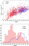 |
Fig. 1. X-ray luminosity and redshift of the X-ray sources. Top panel: X-ray luminosity as a function of redshift for the 1236 X-ray AGN of our sample. Red circles present sources with spectroscopic redshifts available and blue circles those with photometric redshifts. Bottom panel: redshift distributions of photo-z and spec-z sources. The majority of X-ray sources have spec-z at z < 1, whereas at z > 1.5 most of the sources have photometric redshifts. |
The X-ray catalogue is cross-matched with the COSMOS photometric catalogue produced by the HELP collaboration (Shirley et al. 2019, 2021). HELP includes data from 23 of the premier extragalactic survey fields imaged by the Herschel Space Observatory which form the Herschel Extragalactic Legacy Project (HELP). The catalogue provides homogeneous and calibrated multiwavelength data. The cross-match with the HELP catalogue is done using a 1″ radius and the optical coordinates of the counterpart of each X-ray source. In our analysis, we need reliable estimates of the galaxy properties via SED fitting. Therefore, we require all our X-ray AGN to have been detected in the following photometric bands u, g, r, i, z, J, H, Ks, IRAC1, IRAC2, and MIPS/24. IRAC1, IRAC2, and MIPS/24 are the [3.6] μm, [4.5] μm, and 24 μm photometric bands of Spitzer.
2.2. Galaxy reference catalogue
In our analysis, we compare the SFR of X-ray AGN with that of normal, non-AGN galaxies. To perform a fully consistent comparison between the SFR of AGN and non-AGN systems, we apply the same SED fitting analysis in both datasets and require the same availability of photometric bands. The reference catalogue is provided by the HELP collaboration1. There are about 2.5 million galaxies in the COSMOS field. Around 500 000 of these are in the 1.38 deg2 of UltraVISTA (see also Laigle et al. 2016). After excluding X-ray sources, there are about 230 000 galaxies that meet the photometric requirements we have set on the X-ray sample.
3. Analysis
In this section, we describe the SED fitting analysis we applied to measure the galaxy properties. We also estimate the mass completeness of the data at different redshift intervals and describe the selection criteria we apply on the samples. We also examine the reliability of the X-CIGALE calculations.
3.1. X-CIGALE
We use X-CIGALE (Yang et al. 2020, 2022) to measure the properties of the galaxies in our datasets. X-CIGALE is a new branch of the CIGALE SED fitting code (Boquien et al. 2019) that includes new features and improvements. Specifically, X-CIGALE has the ability to model the X-ray emission of galaxies. It can also model the extinction of the UV and optical emission in the poles of the AGN (polar dust). These improvements and their impact on the SED fitting of X-ray AGN have been examined in recent papers (Yang et al. 2020; Mountrichas et al. 2021b,c; Buat et al. 2021).
In the SED fitting analysis, we use the same grid used in Mountrichas et al. (2021a). This allows us to avoid any systematic effects introduced by using different modules and parameter space during the SED fitting process and facilitates a better comparison with the results presented in the Mountrichas et al. (2021a) study. Here, we only summarise the modules included in the fitting process.
A delayed star formation history (SFH) model with a function form SFR ∝ t × exp(−t/τ) is used to fit the galaxy component. The model includes a star formation burst in the form of ongoing star formation that lasts no longer than 50 Myr (Buat et al. 2019). The Bruzual & Charlot (2003) single stellar population template is used to model the stellar emission. Stellar emission is attenuated following Charlot & Fall (2000). The dust heated by stars is modelled following Dale et al. (2014). The SKIRTOR template (Stalevski et al. 2012, 2016) is used for the AGN emission. The same templates and parameter space are used for the X-ray and the galaxy reference sample, including the AGN template (SKIRTOR). The inclusion of the AGN module in the reference catalogue allows us to identify systems with strong AGN component (see Sect. 3.3). All free parameters used in the SED fitting process and their input values are presented in Table 1.
Models and the values for their free parameters used by X-CIGALE for the SED fitting.
As mentioned, X-CIGALE has the ability to model the X-ray emission of galaxies. In the SED fitting process, we use the observed X-ray luminosity in the 2−10 keV band provided by the Marchesi et al. (2016) catalogue. We confirm that using instead the intrinsic (absorption corrected) luminosities does not affect the host galaxy measurements. The photon index, Γ, is fixed to 1.4, which is the value assumed in the Marchesi et al. (2016) catalogue for their luminosity estimations.
3.2. Quality and reliability examination of the fitting results
3.2.1. Quality examination
To restrict our analysis of sources to those with reliable host galaxy measurements, we exclude badly fitted SEDs. For that purpose, we consider only sources for which the reduced χ2,  . This value has been used in previous studies (e.g., Masoura et al. 2018; Buat et al. 2021) and is based on visual inspection of the SEDs. This criterion is satisfied by 89% and 92% of the sources in the AGN and galaxy catalogues, respectively.
To further exclude systems with unreliable measurements of the (host) galaxy properties, we apply the same method presented in Mountrichas et al. (2021a), which has also been adopted in other studies (e.g., Mountrichas et al. 2021c; Buat et al. 2021; Koutoulidis et al. 2022). This method is based on a comparison between the value of the best model and the likelihood-weighted mean value calculated by X-CIGALE. Specifically, in our analysis, we only consider sources with  and
and  , where SFRbest and M*, best are the best-fit values of SFR and M*, respectively, and SFRbayes and M*, bayes are the Bayesian values estimated by X-CIGALE. There are 1236 and 177 245 X-ray AGN and galaxies in the reference catalogue that fulfil these criteria, respectively. In Figs. 2 and 3, we present SEDs of sources that meet the aforementioned criteria (top panels) and of sources that are rejected from our analysis (bottom panels).
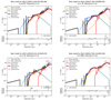 |
Fig. 2. Examples of SEDs of AGN that meet our quality criteria (top panel) and do not satisfy (at least one) of our quality requirements (bottom panel). The AGN SED presented in the left, bottom panel is rejected from our analysis, due to its large |


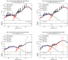 |
Fig. 3. Examples of SEDs of sources in the reference galaxy catalogue that meet our quality criteria (top panel) and do not satisfy (at least one of) our quality requirements (bottom panel). The source with the SED presented in the bottom left panel is rejected from our analysis due to its large |

Furthermore, in our analysis, we take into account the uncertainties of the SFR and M* measurement that X-CIGALE provides. Each source is assigned two weights. One is based on the accuracy, sigma, of the SFR calculation ( ) and the other on the accuracy of the M* measurement.
3.2.2. Reliability examination
Mountrichas et al. (2021a,c) used data from the XMM−XXL and Boötes fields and showed that lack of FIR (Herschel photometry) does not affect the SFR calculations of X-CIGALE. We repeat the same check, using 742 AGN (60% of the total X-ray sample) detected by Herschel. For these sources, we perform SED fitting with and without Herschel bands using the same parametric space. The results are shown in the top panel of Fig. 4. The mean difference, μ, of the SFR measurements is 0.01 and the dispersion is σ = 0.25. We repeat the same exercise for the sources in the reference galaxy catalogue. Approximately 20% of them have Herschel detection. For this sample, the mean difference of the SFR calculations is 0.05 with σ = 0.16 (bottom panel of Fig. 4). The dispersion of the measurements is independent of the AGN obscuration and galaxy extinction. We conclude that lack of FIR photometry does not affect the X-CIGALE SFR calculations.
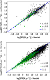 |
Fig. 4. Comparison of SFR measurements with and without Herschel. Top panel: SFR calculations for 742 X-ray AGN with available FIR photometry. The blue dashed line presents the 1:1 relation. Sources at z > 0.5 are shown with black circles, while those at z < 0.5 are shown with green circles. The mean difference of the SFR calculations is 0.01 for the overall population (0.00 for sources at z < 0.5) and the dispersion is 0.25 (0.19 at z < 0.5). Bottom panel: SFR measurements with and without Herschel for sources in the galaxy reference catalogue. The mean difference of the SFR calculations is 0.05 for the overall population (0.04 for sources at z < 0.5) and the dispersion is 0.16 (0.13 at z < 0.5). |
Ultraviolet photometry allows us to trace the young stellar population of galaxies. In our SEDs, we do not include UV (GALEX) photometry because this is available for less than 8% of the sources. At z > 0.5, the u band is redshifted to rest-frame wavelength < 2000 Å, allowing observation of the emitted radiation from young stars. However, low-redshift sources may have inaccurate SFR calculations when both UV and FIR photometry are absent. Our sample includes 88 AGN that lie at z < 0.5. Of these, 70 have FIR detection. These AGN are shown with green circles in Fig. 4. The mean difference in the SFR calculations is μ = 0.00 with dispersion σ = 0.19. For sources at z < 0.5 in the galaxy reference catalogue, the mean SFR difference is 0.04 with σ = 0.13. Therefore, the SFR calculation of sources at z < 0.5 that lack FIR coverage is reliable and we include them in our analysis.
3.3. Identification of non-X-ray AGN systems
As mentioned in Sect. 3.1, in the SED fitting analysis we include an AGN template (SKIRTOR) when we fit the galaxy reference catalogue. This enables us to identify systems with a strong AGN component by measuring the AGN fraction parameter, fracAGN, of X-CIGALE. fracAGN is defined as the ratio of the AGN IR emission to the total IR emission of the galaxy (1 − 1000 μm). We exclude galaxies with fracAGN > 0.2 from the reference catalogue. For comparison, the median fracAGN of the X-ray sample is 0.36. Approximately 33% of sources in the galaxy catalogue are rejected. The fraction rises from lower (∼13% at z < 1.0) to higher (50–60% at z > 1.5) redshifts. This increase is partially due to the fact that AGN tend to reside in more luminous systems that are found at higher redshifts (Fig. 5). Moreover, recent observational studies found that the AGN duty-cycle, that is, the probability of a galaxy hosting an AGN within a given X-ray luminosity interval, increases with redshift (e.g., Georgakakis et al. 2017; Aird et al. 2018). This means that 124 815 galaxies are left in the reference galaxy sample.
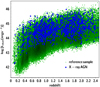 |
Fig. 5. Dust luminosity, Ldust, estimated by X-CIGALE as a function of redshift for sources in the reference catalogue (green points) and X-ray AGN (blue points). Ldust increases with redshift, and AGN tend to reside in the more luminous systems at all redshifts spanned by our datasets. |
We note that if we include all sources of the reference catalogue in our analysis regardless of their AGN fraction value, the median SFR of galaxies is log [SFR(M⊙ yr−1)] = 0.54 (median log [M*(M⊙)] = 10.0) compared to log [SFR(M⊙ yr−1)] = 0.59 (median log [M*(M⊙)] = 9.95) when we exclude sources with fracAGN > 0.2. Including these sources in our analysis would increase the SFRnorm values presented in the following section by ≈17% on average. In a similar manner, excluding sources with fracAGN > 0.1 from the reference catalogue would decrease the SFRnorm values by ∼5% compared to those calculated when excluding galaxies with fracAGN > 0.2. These fluctuations of the SFRnorm caused by the choice of the fracAGN values are within the statistical uncertainties of our measurements and do not affect our overall results and conclusions.
3.4. Mass completeness
In our analysis, we study the SFR of X-ray AGN as a function of X-ray luminosity in five redshift bins up to redshift 2.5. To avoid possible biases introduced by the different mass completeness of our datasets at different redshift intervals, we calculate the mass completeness at each redshift bin. For that, we follow the method described in Pozzetti et al. (2010) and apply it to the galaxy reference sample due to its significantly larger size. The same method has been followed in similar studies (Florez et al. 2020; Mountrichas et al. 2021a) and has also been used to estimate the stellar mass completeness of the COSMOS2015 galaxy catalogue presented in Laigle et al. (2016).
First, we estimate the limiting stellar mass, M*, lim, of each galaxy using the following expression:
 (1)
(1)
where M* is the stellar mass of each source measured by X-CIGALE, m is the AB magnitude of the source, and mlim is the AB magnitude limit of the survey. This equation essentially calculates the mass the galaxy would have if its apparent magnitude was equal to the limiting magnitude of the survey for a specific photometric band. We then use the log M*, lim of the 20% faintest galaxies in each redshift bin. The minimum stellar mass at each redshift interval for which our sample is complete is the 95th percentile of log M*, lim.
We follow Laigle et al. (2016) and use Ks as the limiting band of the samples, which has a value Ks = 24.7 (see Table 1 in Laigle et al. 2016). We find that the stellar mass completeness of our galaxy reference catalogue is log [M*, 95% lim(M⊙)] = 8.60, 9.13, 9.44, 9.69, and 9.97 at z < 0.5, 0.5 < z < 1.0, 1.0 < z < 1.5, 1.5 < z < 2.0, and 2.0 < z < 2.5, respectively. These values agree with those presented in Table 6 of Laigle et al. (2016), although the redshift intervals used are slightly different in the two studies.
3.5. Identification of quiescent systems
The main purpose of this work is to study the position of X-ray AGN relative to the MS as a function of X-ray luminosity and redshift. To this end, we follow previous studies (e.g., Mullaney et al. 2015; Masoura et al. 2018, 2021; Bernhard et al. 2019) and estimate the SFRnorm parameter. SFRnorm is defined as the ratio of the SFR of AGN to the SFR of MS galaxies with similar stellar mass and redshift. However, we want to avoid systematic effects that may have affected previous works that estimated SFRnorm using analytical expressions from the literature to parametrise the SFR of MS galaxies (e.g., Eq. (9) of Schreiber et al. 2015). In our analysis, SFR was calculated in a homogeneous manner, both for the X-ray and the reference catalogues, with the same wavelength coverage which enables us to minimise systematic effects. Thus, we follow the process described in Mountrichas et al. (2021a) to define our own star forming main sequence (SFMS). The goal is not to strictly define the MS, but to exclude in a uniform manner the majority of quiescent systems from our data.
For this exercise, we use the galaxy reference catalogue due to its large size. The outcome of this process is then used in both the galaxy and the X-ray AGN samples to exclude quiescent sources. First, we estimate the sSFR ( ) of each source. Figure 6 presents the distributions of sSFR in each redshift interval. We see that each distribution presents a long tail or a lower second peak at low sSFR values. We consider that these peaks are populated by quiescent systems. Table 2 presents the number of sources in each redshift interval after excluding quiescent systems. Based on our results, ∼10% of the galaxies in the reference catalogue and ∼25% of AGN are quiescent. This result indicates that a larger fraction of X-ray AGN reside in quiescent systems compared to non-AGN galaxies, up to redshift z < 2.5. Moreover, this fraction increases for the X-ray sources from 20% at z > 2 to 40% at z < 0.5. This is in agreement with previous studies that found an increased fraction of AGN hosted by quiescent galaxies at low redshifts compared to higher redshifts (Shimizu et al. 2015; Koutoulidis et al. 2022).
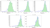 |
Fig. 6. sSFR distributions of the reference galaxy sample, in five redshift intervals. Blue lines present the full distributions. Green areas are the sSFR distribution after applying the sSFR cut, which is defined based on the location of the second, lowest peak of each distribution. |
Number of X-ray AGN and sources in the reference galaxy catalogue after applying the mass completeness limits at each redshift interval.
4. Results
In this section, we compare the SFR of X-ray AGN with the SFR of non-AGN systems in different luminosity and redshift intervals. Next, we examine whether the results of this comparison (also) depend on the stellar mass of the host galaxy.
4.1. SFR of X-ray AGN relative to star forming galaxies as a function of luminosity and redshift
To compare the SFR of X-ray AGN with that of star forming galaxies, we use the SFRnorm parameter. To estimate SFRnorm, we follow the method presented in Mountrichas et al. (2021a). Specifically, the SFR of each X-ray source is divided by the SFR of galaxies from the reference catalogue that have stellar mass that differs ±0.1 dex from the stellar mass of the AGN and lies within ±0.075 × (1 + z) from the X-ray source. The median value of these ratios is used as the SFRnorm of each AGN. In these calculations, each source is weighted based on the uncertainty on the SFR and M* (see Sect. 3.2). We only keep X-ray sources for which the SFRnorm has been estimated using at least 30 galaxies from the reference catalogue. This limit decreases to at least 20 galaxies for the highest redshift bin (2.0 < z < 2.5) and goes down to 10 galaxies when we consider only the most massive systems (11.5 < log [M*(M⊙)] < 12.0, Sect. 4.2).
Figure 7 presents SFRnorm as a function of X-ray luminosity for different redshift intervals. Both for the X-ray sample and the galaxy reference catalogue, quiescent systems have been excluded. In this exercise, we do not present results for the lowest redshift bin (z < 0.5) due to the limited number of X-ray sources. Median values are presented. Errors are calculated using bootstrap resampling (e.g., Loh 2008) by performing 1000 resamplings with replacement at each bin. Results are grouped in LX bins of 0.5 dex. Bins with fewer than 25 AGN are not presented throughout this work. The results do not show dependence of the SFRnorm − LX relation with redshift, in agreement with previous studies (Mullaney et al. 2015; Mountrichas et al. 2021a). However, we notice that the SFR of X-ray AGN appears lower compared to that of star forming galaxies (i.e., SFRnorm < 1). Although this is not statistically significant for some of the bins, it is consistent throughout the luminosities probed by our sample.
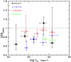 |
Fig. 7. SFRnorm vs. X-ray luminosity. SFRnorm and LX are the median values of our binned measurements in bins of LX with 0.5 dex width. Errors are calculated using bootstrap resampling by performing 1000 resamplings with replacement at each bin. Results are colour coded based on the redshift interval. At all redshifts, SFRnorm does not appear to evolve with LX, at least up to luminosities 2 × 1044 erg s−1 spanned by the X-ray sample. The SFR of X-ray AGN appears lower compared to that of star forming galaxies (i.e., SFRnorm < 1). Although this is not statistically significant for some of the bins, it is consistent throughout the luminosities probed by the dataset. |
As there is no dependence on redshift, in Fig. 8 we present the weighted average SFRnorm in bins of LX over the total redshift range. Mean values are weighted based on the number of sources included in each luminosity bin. Errors present the standard deviation of the measurements. We also plot the results from Mountrichas et al. (2021a) in the Boötes field. The COSMOS X-ray sample spans about an order of magnitude lower luminosities compared to that in Boötes. However, the latter reaches higher LX. This allows us to draw a picture of SFRnorm as a function of Lx for about two orders of magnitude in X-ray luminosity. In the overlapping LX regime, the results from the two studies are consistent. Although the size of the X-ray samples prevents us from drawing strong conclusions, at LX, 2 − 10 keV < 1044 erg s−1, the SFR of AGN appears lower than or equal to that of SFMS, (SFRAGN ≤ SFRSFMS), whereas at LX, 2 − 10 keV > 2 − 3 × 1044 erg s−1 there is an increase in SFRnorm, i.e., SFRAGN ≥ SFRSFMS.
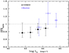 |
Fig. 8. SFRnorm and LX are the mean values of the measurements presented in Fig. 7, grouped in LX bins of 0.5 dex, at all redshifts combined, and weighted based on the number of sources in each bin shown in Fig. 7. Errors represent the standard deviation of SFRnorm and LX in each bin. SFRnorm is systematically lower than one (below the dashed line), which means that at these luminosities the SFR of X-ray AGN is lower compared to that of MS star forming galaxies. In the Boötes field (blue circles), X-ray sources span higher luminosities than their counterparts in COSMOS. In the latter case, SFRnorm values indicate that the SFR of AGN is at least equal to (if not higher than) that of non-AGN systems. |
Overall, our results show no evolution of the SFRnorm − LX relation with redshift. The SFR of AGN is equal to or lower than that of MS galaxies at LX, 2 − 10 keV < 1044 erg s−1 and combining our measurements with those in the Boötes field, there is a hint of an increase in SFRnorm at LX, 2 − 10 keV > 2 − 3 × 1044 erg s−1.
4.2. SFR of X-ray AGN relative to star forming galaxies as a function of luminosity and stellar mass
Previous studies, using either the specific black hole accretion rate parameter (λs, BHAR, Georgakakis et al. 2017; Aird et al. 2018, 2019; Torbaniuk et al. 2021, see also following section) or the specific X-ray luminosity (Yang et al. 2018), found that the stellar mass of the host galaxy may affect how the AGN and galaxy properties are linked. Mountrichas et al. (2021a) found indications that the increase in SFRnorm at LX, 2 − 10 keV > 2 − 3 × 1044 erg s−1 is more evident for AGN that live in galaxies that have stellar masses within a specific range (log [M*(M⊙)] ∼ 11 − 11.5) while the most massive ones do not present this feature in their SFRnorm − LX relation. Moreover, in the previous section, we found that the SFRnorm measurements from the COSMOS X-ray sample are generally lower compared to those in the Boötes field (Fig. 8), but also span lower X-ray luminosities. Another differentiating factor between the two samples is that the X-ray sources in Boötes are more massive than their counterparts in COSMOS because of the higher mass completeness limits of the former sample. In COSMOS, at z < 0.5 the median stellar mass of galaxies that host X-ray AGN is log [M*(M⊙)] = 10.8 and increases to log [M*(M⊙)] = 11.0 − 11.1 at redshift bins higher than z > 0.5, that is, they are about 0.5 dex lower than the AGN hosts in Boötes (see Table 4 in Mountrichas et al. 2021a).
To disentangle the effect of stellar mass, we repeat the measurements presented in the top panel of Fig. 8, but we also group sources in stellar mass bins. In this exercise, we include X-ray AGN at z < 0.5 (52 sources; see Table 2). The number of X-ray AGN available at each stellar mass interval is shown in Table 3. Figure 9 presents the results for four M* bins. At log [M*(M⊙)] < 10.0, the number of AGN is too low to make a meaningful calculation. We notice that, at LX, 2 − 10 keV < 1044 erg s−1, regardless of the stellar mass of their host galaxy, AGN have SFRAGN ≤ SFRSFMS. At LX, 2 − 10 keV > 1044 erg s−1, AGN with 10.5 < log [M*(M⊙)] < 11.0 and 11.0 < log [M*(M⊙)] < 11.5 show enhancement of their SFR compared to MS galaxies. Unfortunately, there are not enough AGN in the COSMOS field with log [M*(M⊙)] < 10.5 and log [M*(M⊙)] > 11.5 at LX, 2 − 10 keV > 1044 erg s−1 to examine whether this trend is also observed in less massive and more massive systems.
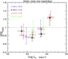 |
Fig. 9. SFRnorm vs. X-ray luminosity. Results are grouped into LX and stellar mass bins of 0.5 dex width. As there is no evolution of the SFRnorm–LX relation with redshift (Fig. 7), measurements are taken at all redshifts spanned by our sample (0 < z < 2.5). The SFRnorm–LX relation appears flat at LX, 2 − 10 keV < 1044 erg s−1. However, at LX, 2 − 10 keV > 1044 erg s−1, SFRnorm, increases with LX. |
Number of X-ray AGN and sources in the reference galaxy catalogue in each stellar mass bin after excluding quiescent systems and applying the mass completeness limits.
In Fig. 10, we complement our measurements in the COSMOS field with those in Boötes from Mountrichas et al. (2021a), in overlapping stellar mass intervals. Mountrichas et al. (2021a) presented their results in different redshift ranges (see their Fig. 11). For the comparison, we re-calculated their SFRnorm values at all redshifts, taking into account the mass completeness at each redshift. The M* intervals in the case of the Boötes dataset are slightly different because of the mass completeness limits of the Boötes dataset. In the 10.5 < log [M*(M⊙)] < 11.0 regime, both X-ray AGN in COSMOS and in Boötes present enhanced SFRnorm at LX, 2 − 10 keV > 1044 erg s−1 compared to that at lower luminosities. However, the results in the Boötes field (blue circles) appear higher compared to those in COSMOS (black circles). We note that due to the mass completeness limits of Boötes, only sources at 0.5 < z < 1.0 contribute to this stellar mass interval. However, in the case of AGN in the COSMOS field, 30% (82 out of 273) of AGN lie at 0.5 < z < 1.0 in this stellar mass range. Although our results in the previous section showed that SFRnorm is independent of redshift, we also plot the results in the COSMOS field for AGN with 0.5 < z < 1.0 (open circles). The measurements are in statistical agreement with those at all redshifts (filled circles), but appear higher and in better agreement with those in Boötes in overlapping LX. Investigating this further, we find that the SFR distribution of sources in the reference catalogue at 0.5 < z < 1 and with 10.5 < log [M*(M⊙)] < 11.0 present a large tail at low SFR values, which could explain the increased SFRnorm values found at this redshift interval. In the middle panel, we present the results for the two fields for AGN that live in galaxies with 11.0 < log [M*(M⊙)] < 11.5. The results in both fields are in agreement. Most importantly, both present a similar increase in SFRnorm at LX, 2 − 10 keV > 1044 erg s−1. In the bottom panel we present measurements for AGN in the 11.5 < log [M*(M⊙)] < 12.0 regime for both fields. In this case, we do not detect enhanced SFRnorm at high luminosities.
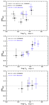 |
Fig. 10. SFRnorm values in bins of LX and stellar mass in the COSMOS field complemented with those found in the Boötes field (Mountrichas et al. 2021a). We only present stellar mass intervals that are similar in the two studies. The small differences in the stellar mass bins are due to the different stellar mass completeness limits of the two surveys. Top panel: in the 10.5 < log [M*(M⊙)] < 11.0 regime, both X-ray AGN in COSMOS and in Boötes, at high luminosities present enhanced SFRnorm compared to SFRnorm at lower luminosities. The results in the Boötes field (blue circles) include only sources at 0.5 < z < 1.0 and appear higher compared to those in COSMOS (black circles). Open circles present the results in COSMOS for AGN with 0.5 < z < 1.0 (open circles). The measurements are in statistical agreement with those at all redshifts (filled circles), but appear higher and in better agreement with those in Boötes in overlapping LX. Middle panel: results for AGN that live in galaxies with 11.0 < log [M*(M⊙)] < 11.5. The results in the two fields are in agreement. Most importantly, both present a similar increase in SFRnorm at LX, 2 − 10 keV > 1044 erg s−1. Bottom panel: measurements for AGN in the 11.5 < log [M*(M⊙)] < 12.0 regime for both fields. In this case, we do not detect enhanced SFRnorm at high luminosities. |
Overall, our results in COSMOS corroborate the findings in the Boötes field for increased SFRnorm at LX, 2 − 10 keV > 1044 erg s−1 compared to lower LX for AGN that live in galaxies with 10.5 < log [M*(M⊙)] < 11.5. A similar trend is not observed for more massive systems. This could be due to different physical mechanisms that fuel the SMBHs of the most massive systems compared to their lower mass counterparts. For example, in massive galaxies, diffuse gas could be accreted onto the SMBH without first being cooled onto the galactic disk (e.g., Fanidakis et al. 2013), whereas in less massive galaxies AGN activity may be triggered by galaxy mergers (e.g., Bower et al. 2006; Hopkins et al. 2008) that also set off star formation. Alternatively, the increase in SFRnorm may occur at higher LX than those probed by the Boötes dataset and ours, for systems with log [M*(M⊙)] > 11.5.
The trends we observe when we split our data into stellar mass bins (in addition to the luminosity bins) are in agreement with those found when we divide our sources only in LX bins (Sect. 4.1), but in the former case the trends are more evident. Specifically, at high luminosities AGN that reside in galaxies with 10.5 < log [M*(M⊙)] < 11.5 seem to have enhanced SFR compared to MS galaxies of similar M*. On the other hand, at lower LX our results show that the SFR of X-ray AGN is lower than or at most equal to the SFR of MS galaxies.
To further examine the correlation between SFRnorm, LX, and M*, we perform a partial-correlation analysis (PCOR). PCOR measures the correlation between two variables while controlling for the effects of a third (e.g., Lanzuisi et al. 2017; Yang et al. 2017; Fornasini et al. 2018). We use one parametric statistic (Pearson) and one non-parametric statistic (Spearman). The results of the p-values are listed in Table 4. The parametric method gives smaller p-values compared to the non-parametric method. This is because of the different assumptions made by the two methods (for more details, see Sect. 3.3 of Yang et al. 2017). Most importantly, p-values for the SFRnorm–M* relation are significantly smaller than the corresponding p-values for the SFRnorm–LX relation, suggesting that SFRnorm correlates stronger with M* than with LX, in agreement with the results presented above.
p-values of partial correlation analysis.
4.3. SFRnorm as a function of specific black hole accretion rate
Mountrichas et al. (2021a) examined the relation between SFRnorm and the λs, BHAR parameter, which quantifies the rate of accretion onto the SMBH relative to the M* of the host galaxy. The results of these authors showed a linear increase in SFRnorm with λs, BHAR. We follow their analysis and compare our calculations using the COSMOS dataset with their measurements. For the estimation of λs, BHAR, we use the analytical Expression (2) of Aird et al. (2018):
 (2)
(2)
where kbol is a bolometric correction factor. We adopt the same value as in Aird et al. (2018), namely kbol = 25. Figure 11 presents the results of our measurements and those from Mountrichas et al. (2021a) for the Boötes field. For the latter, we did not use the averaged values presented in their Fig. 10 (black circles). Instead, we calculated their SFRnorm values at all redshifts spanned by their dataset, taking into account the mass completeness at each redshift. Our results show a mild increase in SFRnorm with λs, BHAR. However, this increase is not as evident as that seen using the Boötes sample. This is confirmed by the expressions that describe the best fit of the measurements. In the case of COSMOS sources, SFR compared to SFR
 for Boötes. Moreover, with the exception of the first two λs, BHAR bins, SFRnorm values of COSMOS AGN appear consistent with but lower than those of the Boötes sources.
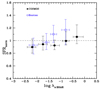 |
Fig. 11. SFRnorm vs. specific black hole accretion rate (λs, BHAR) for sources in COSMOS and in the Boötes field. Median values are presented and the errors are calculated using bootstrap resampling. In both cases, we observe an increase in SFRnorm with λs, BHAR. This is more evident in the case of the Boötes dataset. |
In Table 5, we present the median log λs, BHAR, M*, LX, and redshift of X-ray AGN included in each of the log λs, BHAR bins presented in Fig. 11. Comparing the properties of the AGN between the two datasets, we find that COSMOS sources are less luminous and less massive than their Boötes counterparts in all log λs, BHAR bins. This becomes more evident as we move to higher log λs BHAR values. This could explain the results presented in Fig. 11. The AGN included in the first two log λs, BHAR bins have similar properties (LX, M*) and similar SFRnorm values. For the next two log λs, BHARbins, the SFRnorm is higher in the case of AGN in Boötes compared to those in COSMOS, but in this case Boötes X-ray sources are more luminous and significantly more massive.
Median values of log λs,BHAR, M*, LX, and redshift of X-ray AGN included in each of the log λs, BHAR bins presented in Fig. 11, for sources in the COSMOS and Boötes fields (Mountrichas et al. 2021a).
4.4. Comparison with previous studies
In this section, we compare our results with recent studies. Masoura et al. (2021) found a strong dependence of the SFRnorm with LX (left panel of their Fig. 10) and evolution of the SFRnorm–LX relation with redshift (left panel of their Fig. 11). Although, we do not find a strong dependence of the SFRnorm with LX found in their work, both studies agree that AGN tend to have lower SFR compared to MS galaxies at LX, 2 − 10 keV < 1044 erg s−1, while at LX, 2 − 10 keV ∼ 1044 erg s−1 AGN have similar SFR with MS galaxies. Masoura et al. (2021) results suggest that at higher LX, AGN have enhanced SFR compared to star forming MS galaxies. Although our results show indications for enhanced SFR of AGN compared to the SFR of the galaxy reference catalogue, in particular for AGN hosts with 10.5 < log [M*(M⊙)] < 11.5, the luminosity baseline covered by our COSMOS sample complemented by the Boötes sources used in Mountrichas et al. (2021a) does not extend to sufficiently high LX and with sufficiently a large number of X-ray sources to allow a fair comparison. We leave the comparison at these high luminosities for a future paper where we will make use of the recently released eROSITA X-ray catalogue.
Moreover, our results do not show evolution of the SFRnorm–LX with redshift, in contrast to the findings of Masoura et al. However, an important difference in the analysis used in the two works is that Masoura et al. (2021) compare the SFR of AGN with that of MS galaxies using for the latter the analytical expression of Schreiber et al. (2015). As was shown in Mountrichas et al. (2021a), this approach introduces different systematic errors at different redshift intervals (see their Fig. 6). Therefore, at least to some degree, the different amplitude of the SFRnorm–LX found at different redshifts in Masoura et al. (2021) could be attributed to these systematic effects.
Bernhard et al. (2019) used 541 X-ray AGN in the COSMOS field within 0.8 < z < 1.2. They estimated SFRnorm using the Schreiber et al. (2015) analytical formula and found that higher luminosity AGN, that is, LX, 2 − 10 keV > 2 × 1043 erg s−1, present a narrower SFRnorm distribution compared to their lower LX counterparts. The former is also shifted to higher values, closer to that of MS galaxies. Although the two studies cannot be directly compared due to the different analysis followed (cf. calculation of SFR of MS galaxies), they are in broad agreement in the sense that higher LX AGN seem to have SFR closer to the MS than their lower LX counterparts.
A more fair comparison can be made with Santini et al. (2012). In this latter study, the authors used X-ray-selected AGN in the GOODS-S, GOODS-N, and XMM-COSMOS and compared the SFR of X-ray sources with a mass-match control sample of non-AGN galaxies. Their analysis showed that the star formation of AGN in the COSMOS field (bottom panel of their Fig. 5) is consistent with the star formation of MS galaxies at redshifts 0.5 < z < 2.5, in agreement with our findings.
5. Summary and conclusions
We used approximately 1000 X-ray sources in the COSMOS-Legacy survey (Marchesi et al. 2016) within the UltraVISTA region and compared their SFR with about 90 000 non-AGN systems compiled by the HELP collaboration (Shirley et al. 2019, 2021) over a wide range of redshifts (0 < z < 2.5) and X-ray luminosities (1042.5 < LX, 2 − 10 keV < 1044.0 erg s−1). The galaxy control sample was observed in the same field as the X-ray sources and the same photometric selection criteria were applied to both datasets. We performed SED fitting using X-CIGALE, with the same parametric grid on both datasets to measure (host) galaxy properties. The same mass completeness limits were applied to both samples. These enabled us to avoid systematic errors and compare the SFR of the two populations in a uniform and consistent manner.
First, we studied the SFR–LX relation with respect to the position of the host galaxy on the MS at different luminosity and redshift intervals. Our results show no evolution of the SFR–LX with redshift. The SFR of AGN was found to be lower than or at most equal to the SFR of MS galaxies at LX, 2 − 10 keV < 1044 erg s−1. We complemented our results with those in the Boötes field (Mountrichas et al. 2021a), because the same analysis has been performed in both works. This allows us to extend the luminosity baseline to higher values. We observed a mild increase in the SFR of AGN at LX,2−10keV > 2 − 3 × 1044 erg s−1. At this luminosity regime, AGN appear to have enhanced SFR compared to non-AGN systems.
Prompted by previous studies (e.g., Mountrichas et al. 2021a), we examined the SFR as a function of LX for different stellar mass ranges. The results are consistent with those found when we divide the sources into LX bins. However, when the stellar mass is taken into consideration the trends are more evident. Our results also corroborate the findings in the Boötes field. Specifically, the enhanced AGN SFR is detected for AGN that live in galaxies with 10.5 < log [M*(M⊙)] < 11.5. A similar trend is not observed for more massive systems.
Overall, our results combined with those in the Boötes field show a very mild dependence of SFRnorm on LX, which becomes (more) evident when we take into account the stellar mass of the AGN host galaxies. Specifically, at low and moderate luminosities (1042 < LX, 2 − 10 keV < 1044 erg s−1), AGN tend to have a lower SFR than star forming MS galaxies or they are similar at most. At LX, 2 − 10 keV ∼ 2 − 3 × 1044 erg s−1 and 10.5 < log [M*(M⊙)] < 11.5, AGN present enhanced SFR compared to non-AGN systems.
Although the data used in this work, complemented by those in the Boötes field, span two orders of magnitude in X-ray luminosity, they do not cover the highest LX regime (LX, 2 − 10 keV > 1044.5 erg s−1). AGN at higher LX will allow us to populate the SFR–LX plots with data points at high luminosities and examine whether the SFR of AGN continues to increase as we move to even higher luminosities (LX, 2 − 10 keV > 1045 erg s−1). Ongoing and future surveys (eROSITA, Athena) will provide us with a large number of the most powerful X-ray sources and allow us to answer these questions.
HELP dataset includes sources from the catalogue presented in Laigle et al. (2016). A new catalogue (COSMOS2020; Weaver et al. 2022) was recently released. However, this paper was already in an advanced stage when the new catalogue was made available.
Acknowledgments
GM acknowledges support by the Agencia Estatal de Investigación, Unidad de Excelencia María de Maeztu, ref. MDM-2017-0765. VAM acknowledges support by the Grant RTI2018-096686-B-C21 funded by MCIN/AEI/10.13039/501100011033 and by ‘ERDF A way of making Europe’. This research is co-financed by Greece and the European Union (European Social Fund-ESF) through the Operational Programme “Human Resources Development, Education and Lifelong Learning 2014–2020” in the context of the project “Anatomy of galaxies: their stellar and dust content through cosmic time” (MIS 5052455). The project has received funding from Excellence Initiative of Aix-Marseille University – AMIDEX, a French ‘Investissements d’Avenir’ programme.
References
- Aird, J., Coil, A. L., & Georgakakis, A. 2018, MNRAS, 474, 1225 [NASA ADS] [CrossRef] [Google Scholar]
- Aird, J., Coil, A. L., & Georgakakis, A. 2019, MNRAS, 484, 4360 [NASA ADS] [CrossRef] [Google Scholar]
- Arnouts, S., Cristiani, S., Moscardini, L., et al. 1999, MNRAS, 310, 540 [Google Scholar]
- Bernhard, E., Grimmett, L. P., Mullaney, J. R., et al. 2019, MNRAS, 483, L52 [NASA ADS] [CrossRef] [Google Scholar]
- Boquien, M., Burgarella, D., Roehlly, Y., et al. 2019, A&A, 622, A103 [NASA ADS] [CrossRef] [EDP Sciences] [Google Scholar]
- Bower, R. G., Benson, A. J., Malbon, R., et al. 2006, MNRAS, 370, 645 [Google Scholar]
- Bower, R. G., Benson, A. J., & Crain, R. A. 2012, MNRAS, 422, 2816 [NASA ADS] [CrossRef] [Google Scholar]
- Bruzual, G., & Charlot, S. 2003, MNRAS, 344, 1000 [NASA ADS] [CrossRef] [Google Scholar]
- Buat, V., Ciesla, L., Boquien, M., Małek, K., & Burgarella, D. 2019, A&A, 632, A79 [NASA ADS] [CrossRef] [EDP Sciences] [Google Scholar]
- Buat, V., Mountrichas, G., Yang, G., et al. 2021, A&A, 654, A93 [NASA ADS] [CrossRef] [EDP Sciences] [Google Scholar]
- Cappelluti, N., Brusa, M., Hasinger, G., et al. 2009, A&A, 497, 635 [NASA ADS] [CrossRef] [EDP Sciences] [Google Scholar]
- Charlot, S., & Fall, S. M. 2000, ApJ, 539, 718 [Google Scholar]
- Civano, F., Marchesi, S., Comastri, A., et al. 2016, ApJ, 819, 62 [Google Scholar]
- Dale, D. A., Helou, G., Magdis, G. E., et al. 2014, ApJ, 784, 83 [Google Scholar]
- Dubois, Y., Peirani, S., Pichon, C., et al. 2016, MNRAS, 463, 3948 [Google Scholar]
- Dunn, R. J. H., & Fabian, A. C. 2006, MNRAS, 373, 959 [Google Scholar]
- Elbaz, D., Daddi, E., Borgne, D. L., et al. 2007, A&A, 468, 33 [NASA ADS] [CrossRef] [EDP Sciences] [Google Scholar]
- Fanidakis, N., Georgakakis, A., Mountrichas, G., et al. 2013, MNRAS, 435, 679 [NASA ADS] [CrossRef] [Google Scholar]
- Florez, J., Jogee, S., Sherman, S., et al. 2020, MNRAS, 497, 3273 [NASA ADS] [CrossRef] [Google Scholar]
- Fornasini, F. M., Civano, F., Fabbiano, G., et al. 2018, ApJ, 865, 43 [NASA ADS] [CrossRef] [Google Scholar]
- Georgakakis, A., Salvato, M., Liu, Z., et al. 2017, MNRAS, 469, 3232 [NASA ADS] [CrossRef] [Google Scholar]
- Hickox, R. C., & Alexander, D. M. 2018, ARA&A, 56, 625 [Google Scholar]
- Hickox, R. C., Mullaney, J. R., Alexander, D. M., et al. 2014, ApJ, 782, 11 [NASA ADS] [CrossRef] [Google Scholar]
- Hopkins, P. F., Hernquist, L., Cox, T. J., & Keres, D. 2008, ApJS, 175, 356 [NASA ADS] [CrossRef] [Google Scholar]
- Ilbert, O., Arnouts, S., McCracken, H. J., et al. 2006, A&A, 457, 841 [NASA ADS] [CrossRef] [EDP Sciences] [Google Scholar]
- Koutoulidis, L., Mountrichas, G., Georgantopoulos, I., Pouliasis, E., & Plionis, M. 2022, A&A, 658, A35 [NASA ADS] [CrossRef] [EDP Sciences] [Google Scholar]
- Laigle, C., McCracken, H. J., Ilbert, O., et al. 2016, ApJS, 224, 24 [Google Scholar]
- Lanzuisi, G., Delvecchio, I., Berta, S., et al. 2017, A&A, 602, A123 [NASA ADS] [CrossRef] [EDP Sciences] [Google Scholar]
- Loh, J. M. 2008, ApJ, 681, 726 [CrossRef] [Google Scholar]
- Lutz, D., Mainieri, V., Rafferty, D., et al. 2010, ApJ, 712, 1287 [NASA ADS] [CrossRef] [Google Scholar]
- Marchesi, S., Civano, F., Elvis, M., et al. 2016, ApJ, 817, 34 [Google Scholar]
- Masoura, V. A., Mountrichas, G., Georgantopoulos, I., et al. 2018, A&A, 618, A31 [NASA ADS] [CrossRef] [EDP Sciences] [Google Scholar]
- Masoura, V. A., Mountrichas, G., Georgantopoulos, I., & Plionis, M. 2021, A&A, 646, A167 [EDP Sciences] [Google Scholar]
- McCracken, H. J., Milvang-Jensen, B., Dunlop, J., et al. 2012, A&A, 544, A156 [NASA ADS] [CrossRef] [EDP Sciences] [Google Scholar]
- Morganti, R. 2017, Nat. Astron., 1, 39 [NASA ADS] [CrossRef] [Google Scholar]
- Mountrichas, G., Buat, V., Yang, G., et al. 2021a, A&A, 653, A74 [NASA ADS] [CrossRef] [EDP Sciences] [Google Scholar]
- Mountrichas, G., Buat, V., Yang, G., et al. 2021b, A&A, 646, A29 [EDP Sciences] [Google Scholar]
- Mountrichas, G., Buat, V., Georgantopoulos, I., et al. 2021c, A&A, 653, A70 [NASA ADS] [CrossRef] [EDP Sciences] [Google Scholar]
- Mullaney, J. R., Alexander, D. M., Aird, J., et al. 2015, MNRAS, 453, L83 [Google Scholar]
- Noeske, K. G., Weiner, B. J., Faber, S. M., et al. 2007, ApJ, 660, L43 [CrossRef] [Google Scholar]
- Page, M. J., Symeonidis, M., Vieira, J. D., et al. 2012, Nature, 485, 213 [NASA ADS] [CrossRef] [Google Scholar]
- Park, T., Kashyap, V. L., Siemiginowska, A., et al. 2006, ApJ, 652, 610 [Google Scholar]
- Pozzetti, L., Bolzonella, M., Zucca, E., et al. 2010, A&A, 523, A23 [Google Scholar]
- Rosario, D. J., Trakhtenbrot, B., Lutz, D., et al. 2013, A&A, 560, A72 [NASA ADS] [CrossRef] [EDP Sciences] [Google Scholar]
- Salvato, M., Bolzonella, M., Zucca, E., et al. 2011, ApJ, 742, 61 [NASA ADS] [CrossRef] [Google Scholar]
- Santini, P., Rosario, D. J., Shao, L., et al. 2012, A&A, 540, A109 [NASA ADS] [CrossRef] [EDP Sciences] [Google Scholar]
- Schreiber, C., Pannella, M., Elbaz, D., et al. 2015, A&A, 575, A74 [NASA ADS] [CrossRef] [EDP Sciences] [Google Scholar]
- Scoville, N., Aussel, H., Brusa, M., et al. 2007, ApJS, 172, 1 [Google Scholar]
- Shimizu, T. T., Mushotzky, R. F., Meléndez, M., Koss, M., & Rosario, D. J. 2015, MNRAS, 452, 1841 [NASA ADS] [CrossRef] [Google Scholar]
- Shimizu, T. T., Mushotzky, R. F., Meléndez, M., et al. 2017, MNRAS, 466, 3161 [NASA ADS] [CrossRef] [Google Scholar]
- Shirley, R., Roehlly, Y., Hurley, P. D., et al. 2019, MNRAS, 490, 634 [Google Scholar]
- Shirley, R., Duncan, K., Varillas, M. C. C., et al. 2021, MNRAS, 507, 129 [NASA ADS] [CrossRef] [Google Scholar]
- Speagle, J. S., Steinhardt, C. L., Capak, P. L., & Silverman, J. D. 2014, ApJS, 214, 15 [Google Scholar]
- Stalevski, M., Fritz, J., Baes, M., Nakos, T., & Popović, L. Č. 2012, MNRAS, 420, 2756 [Google Scholar]
- Stalevski, M., Ricci, C., Ueda, Y., et al. 2016, MNRAS, 458, 2288 [Google Scholar]
- Sutherland, W., & Saunders, W. 1992, MNRAS, 259, 413 [Google Scholar]
- Torbaniuk, O., Paolillo, M., Carrera, F., et al. 2021, MNRAS, 506, 2619 [NASA ADS] [CrossRef] [Google Scholar]
- Volonteri, M., Capelo, P. R., Netzer, H., et al. 2015, MNRAS, 449, 1470 [NASA ADS] [CrossRef] [Google Scholar]
- Weaver, J. R., Kauffmann, O. B., Ilbert, O., et al. 2022, ApJS, 258, 11 [NASA ADS] [CrossRef] [Google Scholar]
- Whitaker, K. E., van Dokkum, P. G., Brammer, G., & Franx, M. 2012, ApJ, 754, L29 [Google Scholar]
- Yang, G., Chen, C. T. J., Vito, F., et al. 2017, ApJ, 842, 72 [NASA ADS] [CrossRef] [Google Scholar]
- Yang, G., Brandt, W. N., Vito, F., et al. 2018, MNRAS, 475, 1887 [NASA ADS] [CrossRef] [Google Scholar]
- Yang, G., Boquien, M., Buat, V., et al. 2020, MNRAS, 491, 740 [Google Scholar]
- Yang, G., Boquien, M., Brandt, W. N., et al. 2022, ApJ, 927, 192 [NASA ADS] [CrossRef] [Google Scholar]
All Tables
Models and the values for their free parameters used by X-CIGALE for the SED fitting.
Number of X-ray AGN and sources in the reference galaxy catalogue after applying the mass completeness limits at each redshift interval.
Number of X-ray AGN and sources in the reference galaxy catalogue in each stellar mass bin after excluding quiescent systems and applying the mass completeness limits.
Median values of log λs,BHAR, M*, LX, and redshift of X-ray AGN included in each of the log λs, BHAR bins presented in Fig. 11, for sources in the COSMOS and Boötes fields (Mountrichas et al. 2021a).
All Figures
|
Fig. 1. X-ray luminosity and redshift of the X-ray sources. Top panel: X-ray luminosity as a function of redshift for the 1236 X-ray AGN of our sample. Red circles present sources with spectroscopic redshifts available and blue circles those with photometric redshifts. Bottom panel: redshift distributions of photo-z and spec-z sources. The majority of X-ray sources have spec-z at z < 1, whereas at z > 1.5 most of the sources have photometric redshifts. |
| In the text | |
|
Fig. 2. Examples of SEDs of AGN that meet our quality criteria (top panel) and do not satisfy (at least one) of our quality requirements (bottom panel). The AGN SED presented in the left, bottom panel is rejected from our analysis, due to its large |
| In the text | |
|
Fig. 3. Examples of SEDs of sources in the reference galaxy catalogue that meet our quality criteria (top panel) and do not satisfy (at least one of) our quality requirements (bottom panel). The source with the SED presented in the bottom left panel is rejected from our analysis due to its large |
| In the text | |
|
Fig. 4. Comparison of SFR measurements with and without Herschel. Top panel: SFR calculations for 742 X-ray AGN with available FIR photometry. The blue dashed line presents the 1:1 relation. Sources at z > 0.5 are shown with black circles, while those at z < 0.5 are shown with green circles. The mean difference of the SFR calculations is 0.01 for the overall population (0.00 for sources at z < 0.5) and the dispersion is 0.25 (0.19 at z < 0.5). Bottom panel: SFR measurements with and without Herschel for sources in the galaxy reference catalogue. The mean difference of the SFR calculations is 0.05 for the overall population (0.04 for sources at z < 0.5) and the dispersion is 0.16 (0.13 at z < 0.5). |
| In the text | |
|
Fig. 5. Dust luminosity, Ldust, estimated by X-CIGALE as a function of redshift for sources in the reference catalogue (green points) and X-ray AGN (blue points). Ldust increases with redshift, and AGN tend to reside in the more luminous systems at all redshifts spanned by our datasets. |
| In the text | |
|
Fig. 6. sSFR distributions of the reference galaxy sample, in five redshift intervals. Blue lines present the full distributions. Green areas are the sSFR distribution after applying the sSFR cut, which is defined based on the location of the second, lowest peak of each distribution. |
| In the text | |
|
Fig. 7. SFRnorm vs. X-ray luminosity. SFRnorm and LX are the median values of our binned measurements in bins of LX with 0.5 dex width. Errors are calculated using bootstrap resampling by performing 1000 resamplings with replacement at each bin. Results are colour coded based on the redshift interval. At all redshifts, SFRnorm does not appear to evolve with LX, at least up to luminosities 2 × 1044 erg s−1 spanned by the X-ray sample. The SFR of X-ray AGN appears lower compared to that of star forming galaxies (i.e., SFRnorm < 1). Although this is not statistically significant for some of the bins, it is consistent throughout the luminosities probed by the dataset. |
| In the text | |
|
Fig. 8. SFRnorm and LX are the mean values of the measurements presented in Fig. 7, grouped in LX bins of 0.5 dex, at all redshifts combined, and weighted based on the number of sources in each bin shown in Fig. 7. Errors represent the standard deviation of SFRnorm and LX in each bin. SFRnorm is systematically lower than one (below the dashed line), which means that at these luminosities the SFR of X-ray AGN is lower compared to that of MS star forming galaxies. In the Boötes field (blue circles), X-ray sources span higher luminosities than their counterparts in COSMOS. In the latter case, SFRnorm values indicate that the SFR of AGN is at least equal to (if not higher than) that of non-AGN systems. |
| In the text | |
|
Fig. 9. SFRnorm vs. X-ray luminosity. Results are grouped into LX and stellar mass bins of 0.5 dex width. As there is no evolution of the SFRnorm–LX relation with redshift (Fig. 7), measurements are taken at all redshifts spanned by our sample (0 < z < 2.5). The SFRnorm–LX relation appears flat at LX, 2 − 10 keV < 1044 erg s−1. However, at LX, 2 − 10 keV > 1044 erg s−1, SFRnorm, increases with LX. |
| In the text | |
|
Fig. 10. SFRnorm values in bins of LX and stellar mass in the COSMOS field complemented with those found in the Boötes field (Mountrichas et al. 2021a). We only present stellar mass intervals that are similar in the two studies. The small differences in the stellar mass bins are due to the different stellar mass completeness limits of the two surveys. Top panel: in the 10.5 < log [M*(M⊙)] < 11.0 regime, both X-ray AGN in COSMOS and in Boötes, at high luminosities present enhanced SFRnorm compared to SFRnorm at lower luminosities. The results in the Boötes field (blue circles) include only sources at 0.5 < z < 1.0 and appear higher compared to those in COSMOS (black circles). Open circles present the results in COSMOS for AGN with 0.5 < z < 1.0 (open circles). The measurements are in statistical agreement with those at all redshifts (filled circles), but appear higher and in better agreement with those in Boötes in overlapping LX. Middle panel: results for AGN that live in galaxies with 11.0 < log [M*(M⊙)] < 11.5. The results in the two fields are in agreement. Most importantly, both present a similar increase in SFRnorm at LX, 2 − 10 keV > 1044 erg s−1. Bottom panel: measurements for AGN in the 11.5 < log [M*(M⊙)] < 12.0 regime for both fields. In this case, we do not detect enhanced SFRnorm at high luminosities. |
| In the text | |
|
Fig. 11. SFRnorm vs. specific black hole accretion rate (λs, BHAR) for sources in COSMOS and in the Boötes field. Median values are presented and the errors are calculated using bootstrap resampling. In both cases, we observe an increase in SFRnorm with λs, BHAR. This is more evident in the case of the Boötes dataset. |
| In the text | |
Current usage metrics show cumulative count of Article Views (full-text article views including HTML views, PDF and ePub downloads, according to the available data) and Abstracts Views on Vision4Press platform.
Data correspond to usage on the plateform after 2015. The current usage metrics is available 48-96 hours after online publication and is updated daily on week days.
Initial download of the metrics may take a while.